Optimization of Shipyard Space Allocation and Scheduling ...

Journal of Marine Science and Technology manuscript No.(will be inserted by the editor)

Optimization of Shipyard Space Allocation and Schedulingusing Heuristic Algorithm

J-D. Caprace · C. Petcu · M.G. Velarde · P. Rigo

Received: date / Accepted: date

Abstract In this paper we describe the development

of a tool that allows planners to efficiently and effec-

tively plan space within valuable areas of a shipyard.

Traditionally, space is considered as resource; however,

it is difficult to accurately account for and plan its

consumption with the current available planning soft-

ware’s. The spatial scheduling tool described in this pa-

per can be used by planners to manually or automati-

cally reserve space within the shipyard for construction

of large blocks over the entire erection period of the

ship. The software is coupled with a heuristic optimiza-

tion solver which is inspired by an algorithm used for

”3D bin-packing problems”. The result is the ability to

efficiently generate and compare multiple space alloca-

J-D. CapraceFormerly at ANAST – University of Liege, Actually at FIM-CBOR – Escuela Superior Politecnica del Litoral (ESPOL),Guayaquil, EcuadorTel.: +593-84910928E-mail: [email protected]: [email protected]

C. PetcuANAST – University of Liege, 1 Chemin des chevreuils, 4000Liege, BelgiumTel.: +32-4-3669569Fax: +32-4-3669133E-mail: [email protected]

M.G. VelardeFIMCBOR – Escuela Superior Politecnica del Litoral (ES-POL), Guayaquil, EcuadorTel.: +593-99887755E-mail: [email protected]

P. RigoANAST – University of Liege, 1 Chemin des chevreuils, 4000Liege, BelgiumTel.: +32-4-3669366Fax: +32-4-3669133E-mail: [email protected]

tion alternatives in a reduced time with the ultimate

goal of maintaining the critical ship erection schedule.

Better solution than manual or semi-automatic alloca-

tion of blocks can be obtained through the optimization

module.

Keywords Space allocation · Optimization · Decision

making · Scheduling · Planning · Shipbuilding · 3D

bin-packing

1 Introduction

1.1 Why space allocation is an issue for shipyards?

The high complexity of ship production, due to the

interaction of many different disciplines (hull construc-

tion, electricity, fluids, interior fitting, propulsion, etc.)

requires an intensive design and a detailed production

planning where most of the tasks are carried out in par-

allel. [1] highlighted that it is necessary to increase the

number of simultaneous tasks in order to obtain the

best quality, the lowest price, and the shortest manu-

facturing lead time during the ship production process.

Today, shipyards change their design method in or-

der to increase the number of simultaneous tasks with

the use of more structural blocks (modular construction

strategy). Traditionally, the majority of the design de-

cisions were taken based on experience and opinion of

the designers. These decisions have a strong influence

on production costs, but subsequently on the ship’s per-

formance during its life.

One of the most significant observations for the last

decades concerning shipbuilding is the increase in size

of the ships as shown for passenger ships on Fig. 1. In

2 J-D. Caprace et al.

addition, making a weld in a workshop is much cheaper

than doing the same weld in the dry dock (worse access

conditions, welding overhead, slower welding process,

etc.). The consequence is an increase of the block size

and/or the number of blocks while the working surface

is almost equal. Moreover, most of the time, it is not

possible to enlarge these working surface. It follows that

we arise to a space allocation problem.

Fig. 1 Largest passenger ship size (GT) during the ages - [2]

The assembly of big elements requires necessary avail-

able area within the fabrication workshop to perform

the production. As the blocks become larger and heav-

ier, production space in the shipyard becomes a con-

straint. The largest blocks are limited in the space where

they can be produced due to the lifting and handling

limits. For this reason, it is important to accurately

plan the space in these areas to ensure that blocks are

moved only when and where necessary, to efficiently use

the available space. Unnecessary moves result in non

value-added cost to the block. However, due to produc-

tion constraints and aggressive construction schedules,

maximizing the number of blocks in an area may re-

sult in unnecessary moves, while minimizing unneces-

sary moves results in a less efficient use of the space.

The limited space available in shipyards, as we can see

on Fig. 2 for the Uljanik shipyard in Pula (Croatia),

and the growth in the size of blocks and sections forces

the planners to optimize the use of the available surface

within the workshops and storage areas.

Fig. 2 Limited working space in Uljanik shipyard island(Pula – Croatia)

1.2 Current practice

Spatial scheduling is still currently being done by small

groups of experienced people using tools such as Computer-

Aided Design (CAD), PowerPoint, or Excel and sched-

ule information from their planning systems. Although

these ad-hoc tools are relatively effective, they are cum-

bersome and require a significant amount of time to

update even for minor schedule changes. In addition,

scheduling practices and lessons learned over time are

contained within the experts themselves. In addition,

this knowledge is lost and must be reacquired by yet

another generation of new employees. Providing some

innovative solution to capture this knowledge and auto-

mate the process with a ”smarter tool” would provide

a more efficient allocation of the valuable production

space in each of the construction areas facilities.

Research related to optimal block allocation schedul-

ing in shipbuilding is not prevalent, even though it is

possible to increase the productivity of shipyards and

to decrease the building cost of a ship through efficient

use of space resources. However, some recent research

shows a growing interest of shipyard to improve the

space utilization inside workshops.

In Korea, simulation based production scheduling is

growing up, which can contribute to improve produc-

tion scheduling and planning works and evaluate vari-

ous production scenarios, [3]. To make most use of the

Optimization of Shipyard Space Allocation and Scheduling using Heuristic Algorithm 3

simulation, coupling optimization with simulation is ex-

pected to be far more effective to improve the planning

quality as well as to reduce the efforts in production

planning and control, [4] and [5].

To solve the specific problem various heuristic-based

algorithms have been developed to optimize the block

assignment and space allocation. [6] present a schedul-

ing algorithm using partial enumeration and decom-

position to generate a spatial allocation plan. [7] pro-

posed an optimization of block allocation in assem-

bly area, using simulated annealing method, [8] and

[9], blocks allocation optimization in the assembly area

based on CST (Constraints Satisfaction Technique) and

[10] optimized block division planning using genetic al-

gorithm and product model. Similarly, [11], [12] and [13]

proposed a semi-automated scheduler to increase the

utilization of work area space. Utilizing the similarity

of the two-dimensional packing problem, [14] recently

present a bottom-left-fill heuristic method for spatial

planning of block assemblies.

As presented before, a large spectrum of researches

has been conducted to investigate various algorithms

for optimal configuration and develop decision support

systems for spatial scheduling of dynamic block assem-

bly. However, all the studies deal with a limited number

of production constraints which hardly reflect the real-

istic production situation. For instance, it can be desir-

able to keep some blocks together during the assembly

stage, or place some blocks only in one type of assem-

bly shop, or at the exit gate, or near the ship which are

currently erected, etc.

The paper is organized as follows. After a literature

review on relevant research work, a systematic frame-

work for look-ahead scheduling mechanism is presented,

wherein a heuristic-based algorithm for optimizing the

spatial layout of block assemblies is developed. A case

study with computational experiment is then presented

to demonstrate the proposed approaches.

2 Space allocation issue

2.1 Similarities with other theories

The dynamic allocation of space in the shipyard is

an immensely difficult and time-consuming effort. The

difficulty in scheduling floor space, or spatial schedul-

ing, arises in the fact that the space allocation for one

block significantly affects the availability of floor space

to every other block. Scheduling production space to

satisfy an erection schedule becomes even more com-

plex when unexpected changes of the schedule occur

(e.g., upstream process delays, weather-related delays,

or subcontractor timeliness), [11] and [12]. This illus-

trates a need for a tool that can assist planners in

not only generating efficient spatial layouts, but also

modifying these plans accordingly with minimal ad-

ditional effort. Not only is the practice of scheduling

space a difficult problem, but also the automatic or

semi-automatic scheduling of the space is even more

difficult.

The space allocation issue looks like a cutting stock

problem. The cutting stock problem is a well under-

stood problem in the shipbuilding industry. Steel pro-

cessing facilities in almost every shipyard use nesting

software to determine the best allocation of steel plate

area for cutting out profiles. Having this technology,

the allocation of steel plate space is much more efficient

and results in reduced steel waste. Solution procedures

to the two-dimensional cutting stock problem have and

continue to be developed to improve the efficiency and

computation time of the plate layout.

This issue can also be considered with the conventional

three-dimensional bin packing problem (3D-BPP) where

cubes or solid boxes are ”packed” into a larger empty

container in an effort to maximize the number of boxes

in the container; see Fig. 3 and e.g. in [15]. In the ship-

building context, the working area, platen, or shop floor

length, width and height are considered the ”X”, ”Y”

and ”Z” dimensions of the container and the ”t” di-

mension is the time schedule horizon. The problem is

thus more complex than a simple 3D bin-packing prob-

lem: there are three geometric dimensions and in addi-

tion, the time dimension. In order to simplify the prob-

lem, only two geometrical dimensions (floor length and

width) are generally considered additionally to the time

dimensions. The objective, as defined by the shipyard

managers, is thus to maximize the number of building

blocks produced in a given surface over a certain time

horizon. In the sequel, we refer to this problem as the

Space and Time Allocation (STA) problem.

Only few solution procedures have been developed for

these types of problems, [8], [17], [18] and [19], and opti-

mal solutions procedures have proved to be NP-hard be-

cause of the exponential explosion of the solution space,

[20]. I.e. an ”optimal solution” for a large application

cannot be found within reasonable computing times.

Therefore, the user should accept obtaining a ”nearly

optimum” solution. An efficient tool should make use

of modern heuristics to find such results within short

computing time.


There is one key difference between shipyard spatial

scheduling and the conventional ”bin-packing” prob-

lem. In the bin-packing problem, it is generally assumed

that the blocks to be packed are all available at time 0.

In the shipbuilding industry, the blocks become avail-

able for placement at different times. Also, the general

case of the academic problem is not relevant in the prac-

tical sense due to the fact that the ”real-world” system

has significantly more complex constraints than those

of the general case. Some of these constraints include

preferred locations, spacing between the units, schedule

requirements, and so forth.

[21], [22], [15] and [23] are recent contributions which

provide brief surveys of the literature on 3D-BPP. Since

the problem is hard, most efficient approaches rely on

local search metaheuristics for the solution of large-

scale instances. In particular [22] have proposed a Guided

Local Search (GLS) heuristic for 3D-BPP. In their com-

putational experiments, this approach appears to out-

perform the best available heuristics for 3D-BPP. It also

offers a high degree of flexibility in its implementation,

so that it can be easily adapted to variants of the prob-

lem involving different objective functions and/or ad-

ditional constraints. Therefore, the algorithm that we

have developed for STA explicitly builds with the aid

of their work.

2.2 Challenges of space allocation issue

The dynamic allocation of blocks in shipyards is a

huge, difficult and time-consuming effort. The difficulty

in space allocation arises in the fact that:

– The allocation of space to one block significantly

affects the availability of floor space for the other

blocks, [11]. Scheduling production space to satisfy

Fig. 3 3D bin-packing problem in a container - [16]

an erection schedule becomes even more complex

when unexpected changes of the schedule occur (e.g.,

upstream process delays, weather-related delays, or

subcontractor timeliness).

– The allocation of space in a industrial environment

is an issue with different complex production con-

straints:

– Block height might be important because, some-

times, blocks have to be moved by a crane bridge

above others blocks.

– Spacing between blocks might be required for

safety and accessibility reasons.

– Spacing below blocks might be required for trans-

portation with skid platforms.

– Space above blocks might be required for the

movement of other blocks.

– Preferred location for some blocks might be re-

quired to allocate blocks close to specific tools

or equipments.

– Etc.

This illustrates the need for a flexible tool that can

assist planners in, not only generating optimal spatial

layouts, but also modifying day after day these plans

according to the variation of the initial schedule (de-

lays, unplanned maintenance, etc.). The next section

describes the approach that has been developed to help

in the allocation and planning of floor space within the

shipyard.

3 Approach

The objective of the tool described in this paper isto increase the utilization of working area, while main-

taining production schedules. An innovative approach

has been developed in order to include the following

features:

– The automatic allocation of activities (blocks, sec-

tions, panels, etc.) in the workshops;

– The minimization of the wasted surface;

– Long-term and day-to-day simulations in order to

find how a delay impacts the global planning;

– The post-processing of the result in order to allow

a fast decision making (floor plan printing, display

of working load and working force charts, display of

surface utilization charts, etc.).

This tool should thus provide planning proposals, i.e.

a location and a starting day for each block. Unfortu-

nately, it may happen that the available surface in the

assembly hall is not sufficient to produce the entire set

of blocks. The tool should then try to help the user to

take the most efficient decision.


For simplification reasons, no details will be taken into

account regarding the production processes. It is also

assumed that blocks have their final shape during the

assembling process. We don’t take into account the suc-

cessive assembly stages. In addition, a block is consid-

ered to have a parallelepiped shape. Many blocks are

indeed almost parallelepipeds and other shapes could

be considered using the same optimization technique.

Dealing with simple data is more convenient, and we

knew that a decision tool is only efficient if it keeps

things easy to use, even if complex methods are used

to solve the problem. Indeed, the software would lose

part of its power and efficiency if the time needed to

prepare the data becomes excessive. In addition, the

ability to make changes quickly and to view the impact

of those changes in real time provides a tool that will

significantly reduce the cost of planning and replanning.

The first phase of the tool development is the devel-

opment of a Graphical User Interface (GUI) to assist

the planner in his tasks. The second phase of the tool

development focuses on capturing the knowledge of the

planner and using it to implement an automated opti-

mization module. The following sections provide further

details on these two phases of the tool development: the

GUI and the automated optimization scheduling proce-

dure. Finally we present an industrial case study and a

set of conclusions.

4 Required data for optimization

Both the data related to the shipyard’s facilities and

to the production activities (ship blocks, sections, etc.)

are required in order to define the problem.

4.1 Shipyard facilities

The assembly surfaces of a shipyard contains often

more than one working area Ak, for k = 1, 2, · · · ,mof rectangular shape, such as section assembly halls,

block assembly areas, painting halls, outfitting areas,

etc. Different activities on the block are processed in

these areas. Each working area could contain different

preferential zones in order to perform the activity in

a specific place of the workshop rather than another.

Subsequently, three different level of information should

be considered: the workshop, the working area and the

preferential zone.

The main information required about the shipyard fa-

cilities are:

– The available space in the working areas (length L,

width W , height H) of the workshop, see Fig. 4;

– The crane capacities (maximum load, height under

the hook C);

– The definition of preferential zones q inside the work-

shop (length, breadth, height, type of work, etc.);

– The position of the gates;

– The industrial calendar (working days for each ship);

– The personal availability over time.

Fig. 4 Working areas and blocks

It is imperative to know the location of the gates in

the assembly hall and the crane bridge height. Indeed,

it may happen that a particular block cannot be taken

out because other high blocks are on its way to the gate

and the height of the crane bridge may not be sufficient

to pass over them (crane hook constraint). If blocks are

too heavy for the crane bridge, they need to be driven

out on a skid platform. In this case, no block at all

should remain on the way and supports for blocks have

to be elevated in order to let the skid platform get under

the block.

4.2 Production activities

Basically, the input data of the software may be sum-

marized as a list of n ”activities”. Each activity repre-

sents a certain work to be done on a particular block

j = 1, 2, · · · , n. Hence, the following information that

can be provided by the Enterprise Resource Planing

(ERP) system of the shipyard is required:

– Description of the block – block identification, ship

identification, comments, etc.;

– Prismatic dimensions of each block – length lj , width

wj , height hj , for j = 1, 2, · · · , n and related spaces

allocated to movements around the blocks. Blocks

are considered as parallelepipeds. The major reason

for this assumption is that this data is very easily


available; it is easier to deal with basic shapes and

their representations on a surface are more easily

interpretable. This idea does not affect drastically

the results since most blocks have indeed a (almost)

parallelepiped shape. For accessibility and security

reasons, a certain distance may be required between

nearby blocks in the assembly hall. Therefore, an ex-

tra length, an extra width and an extra height can

be considered;

– Position of the block xj and yj – these parame-

ters are coordinates representing the position of the

upper-left corner of block j in the selected area aj ;

– Processing time tj – Processing time interacts with

two aspects: the total amount of workforce needed

for each block and the duration of work. At this

stage of the planning, a precise processing time can-

not be assessed; therefore the processing time has to

be estimated. An estimation of the total amount of

man-time needed is available, thus the processing

time is computed by dividing this man-time by the

available number of workers. The workload assess-

ments become more precise over time. In addition

to the processing time of an activity, some times

may be required to prepare the appropriate surface

and build up supports for blocks or to dismantle

them. This work has no effect on the start and the

end date. Therefore it has to be taken into account

separately;

– Date of production of each block – In this case, the

earliest starting date also called release date rj is

used (earliest date at which production can start

because the required parts are available for assem-

bly) and the latest end date also called due date dj(the date at which the activity of the block has to

be delivered). See Fig. 5;

– Starting date sj ∈ {rj , · · · , dj−tj} – this parameter

indicates the starting date of the assembly of block

j;

– Area aj ∈ {1, 2, · · · ,m} – this parameter indicates

the working area where the block j will be produced.

In some cases, the values may be restricted to a sub-

set of the sections, depending on block characteris-

tics.

– Orientation oj ∈ {0, 1, 2, 3} – this parameter indi-

cates the orientation of the block j in the selected

area a. Blocks can have 4 orientations turning by 90

degrees.

– Subcontractor possibility bj ∈ {0, 1} – this param-

eter indicates whether activity j will be produced

inside the shipyard (bj = 0) or whether it will be

subcontracted (bj = 1). During optimization, these

blocks will preferentially be selected to be produced

in other workshops if the assembly area is over-

loaded;

The following optional additional information can be

defined by the user to improve the quality of the schedul-

ing solutions:

– Fictitious block cj ∈ {0, 1} – this boolean param-

eter indicates that a block is dummy. This option

gives the possibility to introduce zones temporarily

reserved for activities different from block mounting

operations (e.g. storing the ship engines on the as-

sembly shop, temporary space required for cranes,

etc.). The fictitious blocks are only used to reduce

the available space during a definite time window.

– Target date fj - this option allows the user to give a

preferential start date for the optimization module.

If this date cannot be reached by the optimizer, the

trend will be to approach it as best as possible; On

one hand, if we put the target date on the early start

date, we can perform the space allocation with the

”as soon as possible” rule, and on the other hand,

if we put the target date on the latest start date,

we perform the space allocation with the ”as late as

possible” rule.

– Group of blocks gj – several blocks can be grouped

so that the optimizer will find a position for them as

if they are a single unit. The advantage is that we

can simulate the impact of the production of blocks

nearby similar ones. Thus the optimization module

takes into account a group of blocks as a huge block.

A snap tool was implemented to link several blocks

together;

– Preferential zone qj – This field indicates the zone

in which it is preferable to produce the blocks;

– Ship zone pj – This field indicates the zone of the

ship to which the blocks belongs. During the opti-

mization we are trying to group the block from the

same ship zone together to decrease the movements

of the gantry crane;

Fig. 5 Date and duration of an activity


5 The Graphical User Interface (GUI)

The first part of the tool is an interface for the user

(usually a planner or construction manager) to inter-

act with the block attributes, schedule information, and

the actual placement of the units within a production

working area. A color code is used to show the different

status of the blocks.

The main frame of the GUI is divided into two win-

dows. One is the spatial view of the workshop (top view

of the workshop on a given date) the other is the time-

line view (top view of the workshop with a dimension

in space and a dimension in time). These two frames

interact in order to display the situation of the work-

shop at different dates by the dragging of the daily line

in the time-line view.

5.1 Spatial view of the workshop

This frame (see Fig. 6(a)) simply shows a top overview

of the workshop at a selected date. It is possible that

certain blocks will appear or disappear, depending on

when those blocks were placed and when they are sched-

uled to be complete.

The user can move blocks (drag and drop) inside space

(X and Y) for the day selected. The main blocks at-

tributes like length, width, height, weight and schedule

information such as scheduled start date, planned du-

ration, earliest starting date, latest ending date, actual

start can be edited in a properties windows.

5.2 Time-line view of the workshop

The time-line frame (see Fig. 6(b)) shows an overview

of each working area with an axis for the time (hori-

zontal axis) and another one for a dimension (X or Y

- vertical axis). The user can move blocks along the

temporal and spatial (X or Y) dimension by a simple

drag and drop. However the displacement of the blocks

is limited between the earliest start date and the latest

end date, see Fig. 5. The vertical line can be placed on

a precise day of the time-line and shows the state of all

areas at this date.

5.3 Detection of overlaps

The user is also notified of any collisions between over-

lapping blocks. The tool detects all the collisions and

overlaps between the blocks, not only occurring for the

present time, but also for the entire planning period.

5.4 Towards the automated planning

While the spatial scheduling tool (GUI) provides a

planner with several features to generate efficient spa-

tial plans more rapidly, the actual method of allocat-

ing space is not much different than current shipyard

practices, where block placement decisions are based on

expert-user knowledge. The following section describes

a method to automatically allocate and optimize space

according to heuristic algorithm. While it is nearly im-

possible to capture the entire set of rules, constraints,

and preferences used to generate a near-optimal spatial

layout, the automated scheduler can be used to gener-

ate a valid baseline layout, and the end-user can make

modifications to this layout using the spatial scheduling

tool.

6 Optimization of space allocation

6.1 Optimization variable and objective function

The STA problem consists in orthogonally ordering

the n blocks into the m rectangular areas, without over-

lapping, and so as to respect the time constraints, with

the objective to produce the largest possible number of

building blocks.

To achieve this, we defined the following decision

variables for each block j = 1, 2, · · · , n:

– Position of the block xj and yj ;

– Starting date of the activity sj ∈ {rj , · · · , dj − tj};– The block orientation oj ∈ {0, 1, 2, 3};– The working area aj ∈ {1, 2, · · · ,m};– Subcontractor possibility bj ∈ {0, 1}.

(a) Spatial view at a given date

(b) Time-line view – where the vertical axis represents spatialX dimension and the horizontal axis the time-line

Fig. 6 Main frame of the space allocation optimization tool


In addition, each variable can be fixed so that the

optimization algorithm does not have the opportunity

to modify the value. For example, this feature is used to

define the daily production situation of the workshop

(real block position inside the workshop).

A solution, that is to say an assignment of values to

the above variables, is feasible if the individual and the

collective constraints are met. We call individual con-

straints those which bear on one block only, regardless

of the other blocks. The individual constraints can be

modelled as follow:

1. each block must fit within the with of an area aj :

xj ≥ 0 and xj + [ojwj + (1− oj)lj ] ≤W ;

2. each block must fit within the length of an area aj :

yj ≥ 0 and yj + [oj lj + (1− oj)wj ] ≤ L;

3. each block must fit in its time window: sj ≥ rj and

sj + tj ≤ dj

On the other hand, collective constraints deal with the

interaction between the positions of different blocks. un-

less we mention otherwise, the only collective constraint

is that the blocks may not overlap.

6.2 Algorithm

As previously mentioned our developments are based

on the solutions presented by [22] for the 3D-BPP prob-

lem.

6.2.1 General approach

Let X be any solution of the STA problem, that is, any

assignment of values to the variables aj , xj , yj , oj and

sj for j = 1, 2, . . . , n. We implicitly assume that bj = 1

for all j. While trying to find a feasible schedule, our lo-

cal heuristic search strictly enforces the individual block

constraints, meaning that X always satisfies the con-

straints (1)–(3). On the other hand, we do not enforce

the collective constraints, but we measure the extent of

their violation and these measures are summed in an

auxiliary objective function to be minimized. Without

additional real-life collective constraints, the extent of

the violations can be measured by the total ”volume”[m2 × days

]of pairwise overlaps between the n blocks.

Thus, if we denote by overlapsij(X) the volume of the

overlap between blocks i and j, then the auxiliary ob-

jective function can be formulated as shown in equation

1.

f(X) =∑

1≤i<j≤n

overlapij(X) (1)

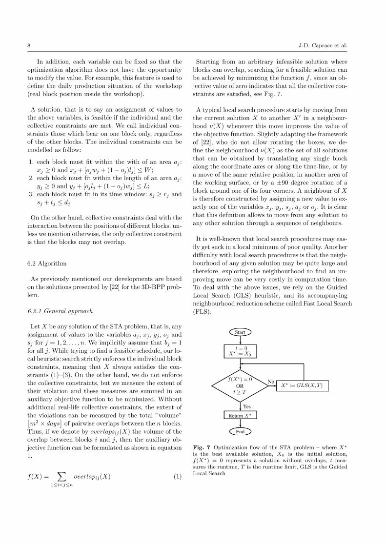
Starting from an arbitrary infeasible solution where

blocks can overlap, searching for a feasible solution can

be achieved by minimizing the function f , since an ob-

jective value of zero indicates that all the collective con-

straints are satisfied, see Fig. 7.

A typical local search procedure starts by moving from

the current solution X to another X ′ in a neighbour-

hood ν(X) whenever this move improves the value of

the objective function. Slightly adapting the framework

of [22], who do not allow rotating the boxes, we de-

fine the neighbourhood ν(X) as the set of all solutions

that can be obtained by translating any single block

along the coordinate axes or along the time-line, or by

a move of the same relative position in another area of

the working surface, or by a ±90 degree rotation of a

block around one of its four corners. A neighbour of X

is therefore constructed by assigning a new value to ex-

actly one of the variables xj , yj , sj , aj or oj . It is clear

that this definition allows to move from any solution to

any other solution through a sequence of neighbours.

It is well-known that local search procedures may eas-

ily get suck in a local minimum of poor quality. Another

difficulty with local search procedures is that the neigh-

bourhood of any given solution may be quite large and

therefore, exploring the neighbourhood to find an im-

proving move can be very costly in computation time.

To deal with the above issues, we rely on the Guided

Local Search (GLS) heuristic, and its accompanying

neighbourhood reduction scheme called Fast Local Search

(FLS).

Fig. 7 Optimization flow of the STA problem – where X?

is the best available solution, X0 is the initial solution,f(X?) = 0 represents a solution without overlaps, t mea-sures the runtime, T is the runtime limit, GLS is the GuidedLocal Search


6.2.2 Guided local search

Generally speaking, GLS augments the objective func-

tion f of a problem to include a set of penalty terms as-

sociated with ”undesirable features” of a solution, and

it considers the new function h, instead of the origi-

nal one, for minimization by a local search procedure.

This procedure is confined by the penalty terms and

focuses attention on promising regions of the search

space. Each time the local search procedure gets caught

in a local minimum, penalties are modified and the lo-

cal search procedure is called again to minimize the

modified objective function. This general scheme has

been adapted to 3D-BPP by [22]. In their precedure,

the features of a solution X are the Boolean variables

Iij(X) ∈ 0, 1, which indicate whether blocks i and j

overlap Iij(X) = 1 or not Iij(X) = 0. The value of the

overlapij(X) measures the impact of the correspond-

ing feature on the solution X. The number of time an

”active” feature has been penalized is denoted by pij ,

which is initially zero. Thus, the augmented objective

function takes the form shown in equation 2, where λ

is a parameter – the only one in this method – that has

to be chosen experimentally.

h(X) = f(X) + λ∑

1≤i<j≤n

pijIij(X)

=∑

1≤i<j≤n

overlapij(X) + λ∑

1≤i<j≤n

pijIij(X)

(2)

Intuitively speaking, Guided Local Search (GLS) at-tempts to penalize the features associated with a large

overlap, but which have not been penalized very often

in the past. More formally, we define an utility function

µij(X) = overlapij(X)/(1 +pij) for each pair of blocks

(i, j). At each iteration the procedure adds one unit to

the penalty pij corresponding to the pair of blocks with

maximum utility, then calls the local search procedure,

see Fig. 8. In a sense, the search procedure forced to

set a higher priority on these features. Since features

with maximum utility keep changing all the time, this

guiding principle prevents GLS from getting stuck in

local minima.

The adaptation of the algorithm has been numeri-

cally validated and tested for several standard test cases

and published in [24] and [25].

6.2.3 Fast local search

The main objective of Fast Local Search (FLS) is to

reduce the size of the neighbourhoods explored in the

local search phase, by an appropriate selection of moves

that are likely to reduce the overlaps with maximum

utility.

To describe the FLS, consider any solution X and any

variable m among the variables xj , yj , sj , aj , oj with

j ∈ [1, . . . , n]. Informally, FLS selects at random a vari-

able m within a list of activate variables, as long as

this list is not empty – active variables are those which

are most likely to lead to an improvement of the cur-

rent solution. The, FLS searches within the domain of

m for an improvement of the objective function. If no

improvement is found, then the variable m becomes in-

active and is removed from the list until the end of the

current call of FLS.

More formally, we define νm(X) as the set of all so-

lutions which differ from X only by the value of vari-

able m. The neighbourhood ν(X) is thus divided into

a number of smaller sub-neighbourhoods as shown in

equation 3.

ν(X) =⋃m

νm(X) (3)

Each of the sub-neighbourhoods νm(X) can be either

active or inactive. Initially, only some sub-neighbourhoods

are active. FLS now continuously visits the active sub-

neighbourhoods in random order, see Fig. 9. If there ex-

ists a solutionXm within the sub-neighbourhood νm(X)

Fig. 8 Optimization flow of the GLS(X,T ) – where X isthe current solution, X? is the best available solution, X0 isthe initial solution, t measures the runtime, T is the runtimelimit, FLS is the Fast Local Search, pij is the penalty for allpairs of blocks, (i, j) is a pair of block, and h(X) is definedin equation 2


such that h(Xm) < h(X), then X becomes Xm; other-

wise we suppose that the selected sub-neighbourhood

will provide no more significant improvements at this

step, and thus it becomes inactive. When there is no

active sub-neighbourhoods left, the FLS procedure is

terminated and the best solution found is returned to

GLS.

Fig. 9 Optimization flow of the FLS(X, (i, j)) – where X isthe current solution, (i, j) is a pair of block, activelist is thelist of the variables associated with the moves applicable toblocks i and j, and to the blocks overlapping either i or j,m? is the best value of m, i.e. the best move reducing morethe objective function, Xm is the solution obtained by settingm := m? in X, and h(X) is defined in equation 2

The size of the sub-neighbourhoods related to the ajand the oj variables is relatively small, therefore FLS

is set to test all the neighbours of these sets. On the

other hand, using an enumerative method for testing

the translations along the x, y, and s-axes would be

very time consuming, especially when areas and/or time

windows are large. We may observe, however, that only

certain coordinates of such neighbourhoods need to be

investigated. Indeed, as pointed out by [22], all overlapij(x)

functions (respectively overlapij(y), overlapij(s) are piece-

wise linear functions, and will for that reason always

reach their minimum in one of their breakpoints or at

the limits of their domains. Thinking of the geometry

of the 3D-BPP, we can easily understand that a best

packing arises either when the boxes touch each other

along their faces, or when they touch the sides of the

bins, see Fig 10. As results, FLS only needs to com-

pute the values of f(x) (respectively, f(y), f(s)) for x

(respectively, y, s) at breakpoints or extreme values. In

fact, there are at most four breakpoints for each overlap

function, and only the first and the last are evaluated.

Once all active moves have been deactivated by the

FLS, two possibilities remain. If the total objective is

null, the process is finished. In the other case all the

moves will become inactive, because no more improv-

ing moves exist. A local minimum is reached and the

FLS iteration is finished. The process starts again at the

first step and as those overlaps cannot be solved, they

will sometimes be selected as the pair having the max-

imum utility. When this occurs, moves of these blocks

are reactivated and their penalties are increased. So, if

we add the penalties to the objective function, the ob-

jective function value of the actual solution will enlarge

and moves improving the objective function will ap-

pear, even if the result will be worse in term of overlap.

But now we have left the local optimum and a better

solution can be found after several iterations.

6.2.4 Selecting the blocks

In the previous sections, we described a GLS heuristic

to find a feasible solution of the STA problem. If GLS

works as expected, then it should return a space and

time allocation with zero overlap, i.e. a feasible solu-

tion, when there is one. In general, however, no such

feasible solution may exist for the set of blocks initially

included in the instance, and we face the problem of se-

lecting a maximum subset of blocks to be scheduled for

assembly. In order to solve this problem we rely on the

following assumption telling that if GLS cannot find a

feasible solution of STA within a predetermined amount

of computation time T , then the heuristic assumption

is that the instance is probably infeasible.

A procedure has been developed allowing to add and

remove blocks from the current set, see Fig. 11. Thus,

assume that, at any iteration of the procedure, X is

a solution (feasible or not) involving some subset of

Fig. 10 Illustration of FLS neighbourhood size reduction


blocks. If the solution GLS(X, T ) returned by GLS is

feasible, then this solution is candidate to be the final

optimal solution. So, we record it if it is better than

the best incumbent solution X∗, and we try to include

an additional block in the set. On the other hand, if

GLS(X, T ) is not feasible, then a fast post-processing

step is performed to produce a feasible solution X ′: this

is achieved by simply removing blocks in a greedy fash-

ion until all overlaps are cancelled. The solution X ′ is

recorded if it is better than the incumbent X∗; then, we

remove an overlapping block from GLS(X, T ) and the

process is repeated. The procedure is stopped after a

predetermined amount of computation time, or by any

more sophisticated stopping criterion, and returns the

feasible solution X∗ involving the largest collection of

blocks.

Fig. 11 Optimization flow of the block selection – where X isthe current solution, X? is the best available solution, X′ is afeasible solution generated by GLS, X0 is the initial solution,t measures the runtime, T is the runtime limit for GLS andTmax is the global runtime limit of the optimization

6.2.5 Additional constraints

The general case of the academic problem is not rel-

evant in the practical sense due to the fact that the

shipbuilding industry has significantly more complex

constraints than those of the general case. Various side-

constraints have to be considered in order to increase

the practical relevance of the STA model. Fortunately,

the GLS framework proved flexible enough to incorpo-

rate most of these constraints without too much addi-

tional effort.

For example, in practice, it may be necessary to re-

strict or to impose the position of certain blocks, e.g.,

because these blocks are already in process when the

planning process is launched, or because some required

handling or production equipment is only available in

a particular area, etc. Such individual constraints on

blocks are easily handled by the GLS algorithm: for-

bidden positions and infeasible neighbours are simply

not generated during the search. Thus, in practice, the

end-user may fix the value or reduce the domain of any

variable when using the software. For instance, he may

prohibit the rotation of some blocks or/and their trans-

lations or/and the working area.

Another industrial constraint that can occur is to al-

locate the preferential zones qj defined in section 4.2

for some specific blocks. In other terms, the GLS will

allocate the block taking into account a certain prior-

ity instead of using a random selection of the blocks.

Other priorities can easily be defined taking into ac-

count other parameters such as the block weight, the

block size or the block complexity.

More complex collective constraints also appeared in

the real-life situation. In particular, for the assembly

halls, each working area has a single door, and the crane

bridge can only carry the blocks up to a certain height

C, see Fig. 12. As a result, it may happen that a tall

block obstructs the door or stands otherwise in the way,

and some blocks may not be delivered in time because

there is no feasible passageway to carry them out of the

hall. Here again, the GLS approach proved ”generic”

enough to deal with this issue. For each generated so-

lution X, we added to the objective function h(X) a

new penalty term which accounts for exit difficulties

as shown in equation 4, where exitij(X) measures the

overlap between block i and the ”exit path” for block

j.

g(X) = h(X) + e(X)

=∑i<j

overlapij(X) + λ∑i<j

pijIij(X) +∑i<j

exitij(X)

(4)

The exit path for j is restricted by security con-

straints which impose to use a straight path, and thus

it is determined by:

– the longitudinal interval [xj , xj + ojwj + (1− oj)lj ];– the transversal interval [0, yj + (1− oj)wj + oj lj ], as

the doors are at position y = 0;

– the vertical interval [C − hj , C], since each block can

be carried up to the height of the crane;


– the completion date sj + tj of block j;

– the area aj where block j is produced.

Note that the value of the exit terms could somehow

be scaled in relation to the h(X) values, but this did

not appear to be useful in our procedure, as the new

penalty terms proved sufficient to drive the objective

function to zero.

Fig. 12 Illustration of overlaps due to crane movements

Additional collective constraints arise when a family

of related blocks have to be produced for a ship. For ex-

ample, all the blocks that include the emergency boats

require similar production equipments, and it is conve-

nient to allocate them to a same zone of the working

area. In a similar way, two blocks that are adjacent in

the ship structure may need to be produced next to

each other in the assembly area, so as to allow a finepositioning of connecting elements such as structural

members or piping tracks. An easy way to cope with

the latter requirement is to define a super-block that

includes the two (or more) adjacent blocks and to re-

place the individual blocks by this super-block in the

data of the problem. With the variable gj described

in section 4.2, several blocks can be grouped so that

the GLS will find a position for them as if they are a

single unit. This parameter doesn’t affect directly the

GLS algorithm but increases considerably the end-user

flexibility. For the first situation, however, this method

is too restrictive, and we preferred instead to define a

”distance” constraint. With the variable pj described

in section 4.2, GLS will minimize the relative distance

between two blocks in order to reduce the undesired

movement of the gantry crane.

Other collective constraints could certainly be included

in the model by taking full advantage of the flexibility

of the GLS framework.

6.2.6 Robustness

The GLS procedure, always starts from an initial solu-

tion X0. A drawback of this approach is that the struc-

ture of X0 can confine the GLS to an area of the so-

lution space that can be difficult to escape (especially

for small values of λ), and therefore, the search process

may not reach the very best solution.

However, in a dynamic industrial setting, this appar-

ent drawback turns out to be an advantage. Indeed,

it may be very costly, or practically impossible for the

company to frequently readjust the schedules and the

allocation of blocks to the working areas. By generating

new solutions from previous ones, the GLS procedure

actually ensures that the structure of previous solutions

can be preserved when the production plans are up-

dated. This is to be contrasted with various methods

proposed for rectangle packing problems, which typi-

cally rely on construction strategies and for which a

slight modification of the data may lead to major per-

turbations of the solution. As a consequence, it may

prove rewarding to run GLS with a relatively small

value of λ in the industrial context.

7 Case study

7.1 Presentation

This case study focuses on the assembly shop of an

European shipyard where relatively small sections (60

∼ 120 tons) are joined together to form huge blocks

(550 ∼ 750 tons). Typically, the ship is then erected in

the dry dock block-by-block until the ship is finished

using a gantry crane.

The modelling of this workshop contains four work-

ing areas (see Fig. 13) as well as the dry dock. The

”bin” is an additional area where blocks are temporary

placed if they are not allocated.

Fig. 13 Layout of the assembly shop considered for the casestudy


A dataset of 268 blocks have been considered where

61 blocks are fictitious and mainly represent part of the

ships in construction in the dry dock, 51 blocks are fixed

and represent the actual situation of the working areas

and finally 156 blocks should be allocated to solve the

STA problem. The surface of the blocks to be allocated

is varying between 200m2 and 1800m2 with an average

of 750m2. The dimensions of the blocks to be allocated

(width and length) are varying between 8.5m and 50m

with an average of 28m. The time period of the dataset

is about 1.5 year. The working duration of the blocks is

varying between 15 and 68 days with an average of 40

days. This dataset correspond to a highly constrained

shipyard STA problem where the space available inside

the workshop is quite similar or superior to the sum of

the block surface.

7.2 Manual and automatic scheduling

Manual allocation of activities. Manually, the user can

drag and drop a non-allocated block from ”bin” area

into an empty working area. Even if an area seems

to be void, another block may have been allocated to

this place some days later. The software detects au-

tomatically such conflicts: critical blocks will directly

change color. A double click on any block shows directly

all block attributes. Multi-selection is also available to

change the value of any parameters for several blocks.

Allocation of activities with the optimization module.

In practice, allocating blocks with the optimization tool

ensures that there is no collision. The optimizer tool

gives always a feasible solution.

While it is nearly impossible to capture the entire

set of rules, constraints, and preferences used by the

planner, the optimization module can be used to gen-

erate a valid baseline layout, and the end-user can make

modifications to this layout using the GUI. The tool of

overlapping detection is very powerful in this case of

manual adjustment of final optimized solution.

If no feasible solution is found by the optimiza-

tion algorithm, the user can directly see which blocks

lead to problems and then choose an adapted solution.

The user can identify the production surface utilization

problems that may happen for the actual data (basi-

cally the fact that not all blocks can be produced in

time). He may for example raise the workforce avail-

ability or subcontract some blocks.

Day to day optimization. The difficulty in space allo-

cation, or spatial scheduling, arises in the fact that the

allocation of space to one block significantly affects the

availability of floor space to the other blocks. Schedul-

ing production space to satisfy an erection schedule be-

comes even more complex when unexpected changes to

the schedule occur (modification of block duration, pro-

duction delays, etc.).

In order to take into account this constraint, we im-

plemented the possibility to fix the attribute of some

blocks so that they cannot be moved by the optimizer.

This functionality is useful to define the starting state

of the workshop: blocks already in the workshop cannot

be moved during the optimization!

Data connection. A link between the current Enterprise

Resource Planning (ERP) system of the shipyard and

the software was also implemented to update all at-

tributes of blocks before an optimization. When a mod-

ification occurs inside the planning (activities duration,

block dimensions, production delays, etc.) the latest in-

formation are always available for the optimization.

7.3 Results and achievements

A comparison between the manual allocation of activ-

ities and the optimization algorithm has been done by

a planner of the shipyard. The planner used a simplistic

allocation rule such as the allocation of the first block

in one corner and processing by rows or by columns.

Nevertheless, we considered some additional constraints

such as the safety distance between the block or the

possibility to rotate the blocks in order to improve the

solution.

The main problem during the allocation of the blocks

is that the planner does not foresee the scheduling of the

blocks along the time. For an optimal allocation of the

activities the optimization algorithm is really helpful.

Tab. 1 as well as Fig. 14 show the relative gains be-

tween the manual and the automatic allocation of the

blocks (optimization algorithm).

We observe in Tab. 1 that the working surfaces are

better used (gain of 12.7%) because more blocks have

been allocated during the same considered period (137

blocks instead of 118 blocks). In the case of the opti-

mized schedule only 19 blocks have not been allocated

while for the manual solution 38 blocks have not been

placed. However, the planner should find a solution to

allocate the remaining 19 blocks that cannot be pro-

duced in time. He may for example raise the workforce

availability to reduce the working duration or subcon-

tract some blocks. Furthermore the average utilization

of the working areas have been improved as shown in

Fig. 14(d).


Both of the solution, i.e. the manual scheduling and

the automatic scheduling, have been considered feasi-

ble by the planner of the shipyard. Nevertheless, he cor-

rected 3% of the position of the blocks for the optimized

solution taking into account additional constraints.

Description Unit Manual Optimized GainSurface used m2 × days 3 593 324 4 115 958 12.7%

Block placed ] 118 137 13.8%

Block not placed ] 38 19 50%

Table 1 Gain between the manual and the automatic allo-cation

In addition the scheduling time is drastically reduced

(hours instead of days). This is probably the most in-

teresting advantage of the developed tool. The planner

considered that the tool can contribute to improve pro-

duction scheduling works and appreciate particularly

that he is now able to evaluate various production sce-

narios in a short time.

For small problems, when space available inside the

workshop is largely superior to the sum of the block

surface, computation times are between 30 and 150 sec-

onds for ∼250 blocks. For more constrained problems,

when the space available inside the workshop is quite

similar to the sum of the block surface, the time re-

quired to find an optimized solution increases from 5

minutes to 1 hour.

Without the tool such planning could take several

days. Consequently another advantage of the tool is

that different schedules can be tested. For instance, if

any production parameter is changed such as the block

splitting or the number of ship to produce simultane-

ously, the impact on the total production time can eas-

ily be studied. These kinds of studies were not possible

manually.

8 Conclusions

In this paper, we have presented a space and time allo-

cation problem arising in large shipyards, and we have

modelled it as a 3-dimensional bin packing problem.

We have demonstrated the main advantages of the

GLS to solve the STA problem:

– Good correspondence between results obtained and

industrial constraints;

– Low computation time (some minutes);

– Four dimensional problems are solved (three spatial

dimensions and one temporal dimension);

– Solution obtained is always feasible;

– If a schedule modification arises and causes an over-

lap between blocks, the algorithm will be able to

solve only locally the issue without modifying the

global solution.

The proposed innovative approach allows a more effi-

cient scheduling for the shipyard. The planner can test

more alternatives and rapidly modify the scheduling to

(a) Time-line – Manual (b) Time-line – Optimized

(c) Number of blocks vs. time

(d) Surface utilization in % vs. time

Fig. 14 Comparison of the time-line results between themanual and automatic allocation, where 14(a) and 14(b)present the time-line view where the vertical axis is the spa-tial X dimension and horizontal axis the time-line and 14(c)and 14(d) present respectively the number of blocks and thesurface utilization ratio in function of time


find the best one. But the preparation and verification

of data for the simulation remain a major stage to en-

sure the reliability of the results.

Gains obtained for the shipyard are substantial. The

workshop productivity by using the new concept is in-

creased as less time is needed for scheduling and a bet-

ter space utilization is achieved.

This generic approach allows incorporating various real-

life constraints and leads to the successful implementa-

tion of a flexible and robust application for the ship-

building industry, but potentially also for other indus-

tries.

9 Future work

The work outlined in this paper presents a new promis-

ing method for shipyard spatial scheduling. Neverthe-

less, several improvements or integrations of new con-

straints could be performed:

– An extension of the rectangular shapes for work-

shops and/or blocks to any shapes. However this

would require a complete overhaul of the software

and his optimization method.

– An implementation of a tool to fit and smooth the

workload of the workshop to the workforce available.

It could be done during the optimization phase as a

multi objective optimization.

– Development of a tool to consider predecessors and

successors for the different activities to be allocated.

References

1. Hugues, O. (1994) Applied Computer Aided Design.Tech. rep., International Ship and Offshore StructureCongress – ISSC, inst. Marine Dynamics, Newfoundland.

2. List of the world’s largest cruise ships.Http://en.wikipedia.org/wiki/.

3. Kim, Y. and Lee, D. (2007) A study on the construc-tion of detail integrated scheduling system of shipbuild-ing process. J. Society of Naval Architects of Korea, 44,48–54.

4. Bair, F., Langer, Y., Caprace, J., and Rigo, P. (2005)Modelling, Simulation and Optimization of a Shipbuild-ing Workshop. COMPIT’05 – The 4th InternationalConference on Computer Applications and InformationTechnology in the Maritime Industries, May, vol. 1, pp.283–293, Hamburg, Germany.

5. Nedeb, C., Friedewald, A., Wagner, L., and Hubler, M.(2006) Simulation of Material Flow Processes in the Plan-ning of Production Spaces in Shipbuilding. COMPIT’06– The 5th International Conference on Computer Ap-plications and Information Technology in the MaritimeIndustries, May, vol. 1, pp. 186–198, Leiden, Netherlands.

6. Park, K., Lee, K., Park, S., and Kim, S. (1996) Modelingand solving the spatial block scheduling problem in ashipbuilding company. Comput. Ind. Eng., 30, 357–364.

7. Okumoto, Y. and Iseki, R. (2005) Optimization of BlockAllocation in Assembly Area using Simulated AnnealingMethod. Journal of the Japan Society of Naval Architectsand Ocean Engineers, 1, 71–76, in Japanese.

8. Lee, K., Lee, J., and Choi, S. (1996) A Spatial Schedul-ing System and its Application to Shipbuilding: DAS-CURVE. Expert Systems with Applications, 10, 311–324.

9. Lee, D., Kang, Y., and Kim, H. (2005) Block AssignmentPlanning for shipbuilding Considering Preference shopand Load Balancing. Proceedings of 12th ICCAS 2005 ,vol. 1, pp. 55–68.

10. Wibisono, M., Hamada, K., Kitamura, M., and Ke-savadey, V. (2007) Optimization System of Block Divi-sion using Genetic Algorithm and Product Model. Jour-nal of the Japan Society of Naval Architects and OceanEngineers, 6, 109–118.

11. Finke, D. A., Ligetti, C. B., Traband, M. T., and Roy, A.(2007) Shipyard space allocation and scheduling. Journalof Ship Production, 23, 197–201.

12. Finke, D. A., Ligetti, C. B., Traband, M. T., and Roy, A.(2008) Activity-based spatial scheduling. Journal of ShipProduction, 24, 12–16.

13. Cho, K., Chung, K., Park, C., Park, J., and Kim, H.(2001) A spatial scheduling system for block paintingprocess in shipbuilding. CIRP Annals - ManufacturingTechnology, 50, 339 – 342.

14. Shin, J. G., Kwon, O. H., and Ryu, C. (2008) Heuris-tic and metaheuristic spatial planning of assembly blockswith process schedules in an assembly shop using dif-ferential evolution. Production Planning & Control , 19,605–615.

15. Martello, S., Pisinger, D., and Vigo, D. (2000) The threedimensional bin packing problem. Operations Research,48, 256–267.

16. Wu, Y., Li, W., Goh, M., and de Souza, R. (2010) Three-Dimensional Bin Packing Problem with Variable BinHeight. European Journal of Operational Research, 202,347–355.

17. Lee, J. K., Lee, K. J., Park, H. K., Hong, J. S., and Lee,J. S. (1997) Developing Scheduling Systems for DaewooShipbuilding: DAS Project. European Journal of Opera-tional Research, 97.

18. Lim, A., Rodrigues, B., and Yang, Y. (2005) 3-D Con-tainer Packing Heuristics. Applied Intelligence, 22, 125–134.

19. Lodi, A., Martello, S., and Vigo, D. (2002) Heuristic Al-gorithms for the Three-Dimensional Bin Packing Prob-lem. European Journal of Operational Research, 141,410–420.

20. Garey, M. R. and Johnson, D. S. (1990) Comput-ers and Intractability; A Guide to the Theory of NP-Completeness. W. H. Freeman & Co.

21. Brunetta, L. and Gregoire, P. (2005) A General PurposeAlgorithm for Three-dimensional Packing. INFORMSJournal on Computing, 17, 328–338.

22. Faroe, O., Pisinger, D., and Zachariasen, M. (2003)Guided local search for the three-dimensional bin-packingproblem. INFORMS J. on Computing, 15, 267–283.

23. Martello, S., Pisinger, D., Vigo, D., Boef, E. D., and Ko-rst, J. (2007) Algorithm 864: General and Robot PackageVariants of the Three-dimensional Bin Packing Problem.ACM Transactions on Mathematical Software, 33, 1–12.


24. Langer, Y., Bay, M., Crama, Y., Bair, F., Caprace, J., andRigo, P. (2005) Optimization of Surface Utilization Us-ing Heuristic Approaches. COMPIT’05 – The 4th Inter-national Conference on Computer Applications and In-formation Technology in the Maritime Industries, May,vol. 1, pp. 419–425, hamburg, Germany.

25. Bay, M., Crama, Y., Langer, Y., and Rigo, P. (2010)Space and time allocation in a shipyard assembly hall.Annals of Operations Research, 179, 57–76.

Optimization of Shipyard Space Allocation and Scheduling ...

Documents

Transcript of Optimization of Shipyard Space Allocation and Scheduling ...