OPTIMIZATION OF ROBOTIC ASSEMBLY OF PRINTED …ethesis.nitrkl.ac.in/2938/1/amu_final_6.pdf ·...
82
OPTIMIZATION OF ROBOTIC ASSEMBLY OF PRINTED CIRCUIT BOARD USING EVOLUTIONARY ALGORITHM A THESIS SUBMITTED IN PARTIAL FULFILLMENT OF THE REQUIREMENTS FOR THE DEGREE OF Master of Technology in Machine Design and Analysis By AMIT KUMAR SHRIVASTAVA Department of Mechanical Engineering National Institute of Technology Rourkela-769008 2011
Transcript of OPTIMIZATION OF ROBOTIC ASSEMBLY OF PRINTED …ethesis.nitrkl.ac.in/2938/1/amu_final_6.pdf ·...

OPTIMIZATION OF ROBOTIC ASSEMBLY OF PRINTED CIRCUIT BOARD USING EVOLUTIONARY
ALGORITHM
A THESIS SUBMITTED IN PARTIAL FULFILLMENT OF THE
REQUIREMENTS FOR THE DEGREE OF
Master of Technology in
Machine Design and Analysis
By
AMIT KUMAR SHRIVASTAVA
Department of Mechanical Engineering National Institute of Technology
Rourkela-769008 2011

OPTIMIZATION OF ROBOTIC ASSEMBLY OF PRINTED CIRCUIT BOARD USING EVOLUTIONARY
ALGORITHM
A THESIS SUBMITTED IN PARTIAL FULFILLMENTOF THE REQUIREMENTS FOR THE DEGREE OF
Master of Technology in
Machine Design and Analysis
By
AMIT KUMAR SHRIVASTAVA (209ME1192)
Under guidance of
Porf. S. S. MAHAPATRA
Department of Mechanical Engineering National Institute of Technology
Rourkela-769008 2011

National Institute Of Technology
Rourkela
CERTIFICATE This is to certify that the thesis entitled, “OPTIMIZATION OF ROBOTIC ASSEMBLY
OF PRINTED CIRCUIT BOARD BY USING EVOLUTIONARY ALGORITHM” submitted by Mr.
AMIT KUMAR SHRIVASTAVA in partial fulfilment of the requirements for the
award of Master of Technology Degree in MACHENICAL ENGINEERING with
specialization in “MACHINE DESIGN AND ANALYSIS” at the National Institute
of Technology, Rourkela is an authentic work carried out by him
under my supervision and guidance.
To the best of my knowledge, the matter embodied in the thesis has not
been submitted to any other University / Institute for the award of
any Degree or Diploma.
Date PROF. S. S. MAHAPATRA
DEPARTMENT OF MECHANICALENGINEERING
NATIONAL INSTITUTE OF TECHNOLOGY
ROURKELA-796008

ACKNOWLEDGEMENT
This project is by far the most significant accomplishment in my life and it would be
impossible without people who supported me and believed in me.
I would like to extend my gratitude and my sincere thanks to my honourable,
esteemed supervisor Prof. S. S. Mahapatra, Department of Mechanical Engineering. He is
not only a great lecturer with deep vision but also most importantly a kind person. I sincerely
thank for his exemplary guidance and encouragement. His trust and support inspired me in
the most important moments of making right decisions and I am glad to work under his
supervision.
I am very much thankful to our Head of the Department, Prof. R. K. Sahoo, for
providing us with best facilities in the department and his timely suggestions. I am very much
thankful to all my teachers Prof. N. Kavi, Prof. D. R. Prahi, Prof. P. K. Ray, Prof. R. K.
Behera, Prof. S. K. Acharya, Prof. S. C. Mohanty, Prof. J. Srinivasan and Prof. S. Datta
for providing a solid background for my studies. They have been great sources of inspiration
to me and I thank them from the bottom of my heart.
I would like to thank all my friends and especially my classmates for all the
thoughtful and mind stimulating discussions we had, which prompted us to think beyond the
obvious. I’ve enjoyed their companionship so much during my stay at NIT, Rourkela.
I would like to thank all those who made my stay in Rourkela an unforgettable and
rewarding experience.
Last but not the least I would like to thank my parents, sister and Shruti Shivastava,
who taught me the value of hard work by their own example. They rendered me enormous
support being apart during the whole tenure of my stay in NIT Rourkela.
Amit Kumar Shrivastava

ii OPTIMIZATION OF ROBOTIC ASSEMBLY OF PRINTED CURCUIT BOARD USING AIS ALGORITHMS
CONTENTS
Acknowledgement i
Abstract iv
List of figures v
List of tables vi
List of Abbreviation vii
1. Introduction 1.1 Introduction 1 1.2 Assembly equipment 4 1.3 Assembly process and Machine description 5 1.4 PCB assembly problems 9
2. Literature review
2.1 Introduction 12 2.2 Placement Sequence 12 2.3 Placement sequencing and feeder assignment 18 2.4 Summary of Literature review 22
3. Techniques for optimization of PCB assembly
3.1 Introduction 24 3.2 Evolutionary Algorithms 25
3.1.1 Introduction 25 3.1.2 Genetic Algorithm 26
3.3 Ant Colony Optimization (ANO) 27 3.4 Particle Swarm Optimization (PSO) 28 3.5 Intelligent Water Drops 30
3.5.1 Introduction 30 3.5.2 Natural Water Drops 30 3.5.3 Intelligent Water Drops 31
3.6 Bee Colony Optimization 32 3.6.1 Introduction 32 3.6.2 Bee Colony Optimization 32 3.6.3 BCO Application 33
4. Theory of Artificial Immune System
4.1 Introduction 35 4.2 Artificial Immune System (AIS) 35 4.3 Theory of AIS 37

iii OPTIMIZATION OF ROBOTIC ASSEMBLY OF PRINTED CURCUIT BOARD USING AIS ALGORITHMS
4.3.1 Immune Network model 37 4.3.2 Negative Selection Algorithm 38 4.3.3 Clone Selection Algorithm 39 4.3.4 Danger Theory 40
4.4 Recently use of AIS modelling 43 4.5 Summary 43
5. Problem Description
5.1 Types of PCB assembly used 45 5.2 Benchmark problems for PCB assembly 47 5.3 Mathematical Model 51 5.4 Development of AIS algorithm 52
5.4.1 Encoding 55 5.4.2 Evaluation of Fitness Function 56 5.4.3 Clone selection Principle 56 5.4.4 Affinity Mutation Principle 57 5.4.5 Receptor Editing 58
6. Results and Discussions
6.1 Result of AIS performance 60 6.2 Comparison with IP model 60 6.3 Effect of receptor editing percentages 62 6.4 Discussion Points 63
7. Conclusions and Future work
7.1 Conclusions 65 7.2 Future works 66 REFERENCES. . . . . . . . . . . . . . . . . . . . . . . . . . . . . . . . . . . . . 67

iv OPTIMIZATION OF ROBOTIC ASSEMBLY OF PRINTED CURCUIT BOARD USING AIS ALGORITHMS
Abstract
This research work describes the development and evaluation of a custom application
exploring the use of Artificial Immune System algorithms (AIS) to solve a component
placement sequencing problem for printed circuit board (PCB) assembly. In the assembly of
PCB’s, the component placement process is often the bottleneck and the equipment to
complete component placement is often the largest capital investment. In printed circuit board
(PCB) assembly, the Production rate of the component placement process is dependent on
three interrelated problem such as sequence of component placement known as component
sequencing problem, assignment of component types to feeders of the placement machine
viewed as feeder arrangement problem, and determination of the cycle time i.e. minimum
time taken by robot to complete the whole assembly. In the world of PCB manufacturing all
the above three issues are playing an important role for increasing the efficiency of
production. In case, some components with the same type are assigned to more than one
feeder, the component retrieval problem should also be considered. The problem of allocating
components to a printed circuit board assembly line, which has several non-identical
placement machines in series, is formulated as a mini-type integer programming (IP) model
in this report. In order to achieve the best production throughput, the objective of the model is
to minimize the cycle time of the assembly line. The model has been proven as NP-
complete(non-deterministic polynomial) and a quick solving tool “LINGO” is used to solve
small problems.
Due to their inseparable relationship we take feeder arrangement as a fixed i.e.
component on feeders are predetermined. We only considered the component sequencing
problem, a hybrid Artificial Immune System (AIS) algorithm is adopted to solve this
problems for a type of PCB placement machines called the sequential pick-and-place (PAP)
machine in this work. The objective is to minimise the total distance travelled by the
placement head for assembling all components on a PCB, The results are compared with the
other researcher’s result used different type of algorithms for same problem.
Keywords: Predefine Feeder arrangement, PCB Assembly, AIS Algorithm, and LINGO.

v OPTIMIZATION OF ROBOTIC ASSEMBLY OF PRINTED CURCUIT BOARD USING AIS ALGORITHMS
List of figures
figure (1.1) Example of Surface Mount line Configuration 5
figure (1.2) Example of configuration of a Chip Shooter Machine 6
figure (1.3) Example Configuration of a Gantry Machine 7
figure (1.4) Example Configuration of a SCARA Robot 8 figure (3.1) The tour with A=>B =>C =>E =>D => A is the optimal tour 24
figure (3.2) Real ant behaviour in finding the shortest path between the 27
nest and the food
figure (3.3) Birds or fish exhibit such a coordinated collective behavior 29
figure (4.1) Presence of paratope and idiotope on antibody 36
figure (4.2) Basic of Negative Selection Algorithm 38
(a) Censoring Stage 38
(b) Monitoring Stage 38
figure (4.3) Basic of Clonal Selection Algorithm. 39
figure (4.4) Principle of Danger Theory 41
figure (5.1) The assembly sequence of PCB with one set of feeder 45
figure (5.2) The assembly sequence of PCB with two set of feeder 46
figure (5.3) The assembly sequence of PCB with turret arrangement 47
figure (5.4) The assembly sequencing of placement head 49
figure (5.5) The Flow chart of artificial immune system algorithm for PCB assembly 54
figure (5.6) Encoding of two links
(a) Encoding of given sequence of component is on PCB 55
(b) Encoding of feeder components 55
figure (5.7) The Pair wise interchange mutation operation 57
figure (5.8) The Inverse mutation operations 58
figure (5.9) The Displacement mutation operation 58
figure (6.1) The Decrement graph between fitness value and iteration number s 61
figure (6.2) Effect of variation in receptor editing percent 62

vi OPTIMIZATION OF ROBOTIC ASSEMBLY OF PRINTED CURCUIT BOARD USING AIS ALGORITHMS
List of tables
Table 1.1 Differences between PAP and CS Machines 2
Table 5.1 Data of integrated problem with 10 components and 6 types 50
Table 5.2 Component type and coordinates of different type of assembly problem 50
Table 6.1 Comparison between AIS and IP model 61

vii OPTIMIZATION OF ROBOTIC ASSEMBLY OF PRINTED CURCUIT BOARD USING AIS ALGORITHMS
Abbreviation and Acronym:
Indices
i,j Components(i,j=0,1,....,n).
t Component type (t=1,2,3...µ)
l Feeders (f=1,2,......µ)
seq Placement order of placement position(p=1,2,3,...n)
Distances-
dol Distance travelled from starting point to feeder l.
dlj Distance travelled from feeder l to position of component j on PCB.
dil Distance travelled from position of component i to feeder l.
dio Distance travelled from feeder l to starting point.
Sub-tour elimination constraint-
Ui Placement order of component i.
Decision variables-
Xij 1 if component i is placed immediately before component j; 0
otherwise.
Xip 1 if component i is placed in the pth position; 0 otherwise.
ytil 1 if component jwith component type t is stored in feeder l; 0
otherwise.
Aberrations PCB Printed circuit board
AIS Artificial immune system
PAP Pick and place machine
Antibody Sequence order of placement of component on board.
Population size Total number of sequence available.

Chapter 1
INTRODUTION
“OPTIMIZATION OF ROBOTIC ASSEMBLY OF PRINTED CURCUIT BOARD USING AIS ALGORITHMS”
2 INTRODUCTION
1.1 Introduction
Wide applicability of printed circuit boards (PCBs) in many electronic devices such as
personal computers, laptops, LCDs, mobile phones, and audio-video equipment has placed an
unprecedented demand for PCBs resulting in to explore strategies for low cost production of
PCBs. Customers’ needs such as smaller product size, greater functionality and reliability
have driven the assembly technologies of electronic components and printed circuit boards
from manual operations to completely automated ones. That is why the manufacturing
industry invests a great amount of resources in order for their processes to be automated by
means of integrating electronic systems to their plants, which usually involves having
efficient techniques to ease the control of production. A major challenge for any
manufacturing industry is to increase its productivity, safety, and quality without significantly
increasing unit cost of production. In past few years, automated and flexible manufacturing
systems have received considerable attention from design engineers and researchers [1.1]
[1.2] as they provide an alternative to anincreased safety, higher productivity and quality of
production. Robots have become an inseparable part of many manufacturing systems,
replacing humans, thereby not only increasing the safety of production but also the
productivity and quality of production.
Actually, a PCB consists of a pattern of electrical traces etched from copper that is
laminated on an insulated base, which is typically rigid fibreglass. The PCB serves as the
interconnection device with electrical currents travelling on the board and the different
discrete electronic components that are essential to the functioning of an electronic product.
Components from a few hundred to some thousands can be assembled on a single Printed
Circuit Board. The operation of placement of various electronic components on a PCB is
called PCB assembly. It can be classified into two categories:
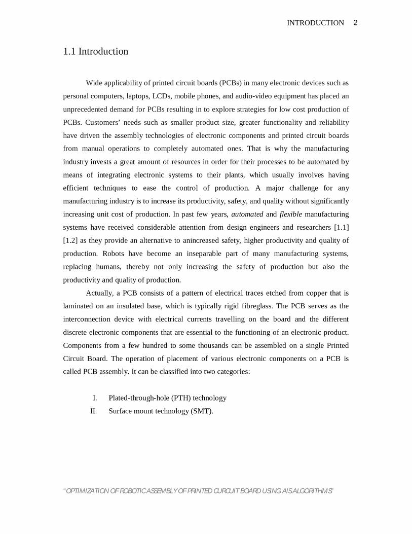
I. Plated-through-hole (PTH) technology
II. Surface mount technology (SMT).
“OPTIMIZATION OF ROBOTIC ASSEMBLY OF PRINTED CURCUIT BOARD USING AIS ALGORITHMS”
3 INTRODUCTION
For products where overall board size is not a serious concern, the PTH technology is
applied. The components are inserted into the holes drilled through the PCB. Then, the
connections are soldered on the underside of the PCB between the component lead and the
PCB pad. However, needs from consumers, such as smaller product size and greater function
and reliability, have forced the SMT to switch the PTH technology. The configuration and the
size of surface mount components have permitted mounting an outsized range of components
on a one PCB.
The assembly of PCBs is a complex task since a PCB may contain many electronic
components in numerous shapes and sizes mounted at specific locations on the board. In the
few past years, board assembly consisted of inserting component leads through holes in the
board and then soldering them into place (Through-Hole assembly). Currently, Surface
Mount Technology (SMT) is mostly used in PCB assembly. With SMT, components are
attached to a vacant board with solder paste at pre specified location. Then a reflow operation
heats the boards inflicting the solder paste to melt and form the proper connections [1.3]. A
SMT assembly line mounts the components at faster speeds and with higher precision than a
Through-Hole assembly line.
The PCB assembly process within the SMT atmosphere consists of 5 operations. 1st
of all, solder paste is applied where the components are going to be placed. Typically, it is
applied by screen printing [1.4]. Then, it is followed by the positioning operation of
component. A high-speed placement machine is employed to mount tiny components likechip
resistors on the PCB 1st. A flexible placement machine is then used to mount massive and
large components such as integrated circuits (ICs) on the Printed circuit board. Finally the
components areassembled; the PCB is inspected for missing components. Subsequently, the
PCB is conveyed through an oven, which makes the solder paste reflow and form the solder
joints. Finally, the PCB should be cleaned to remove the contaminants exposed throughout
fabrication and assembly.

“OPTIMIZATION OF ROBOTIC ASSEMBLY OF PRINTED CURCUIT BOARD USING AIS ALGORITHMS”
4 INTRODUCTION
1.2 Assembly Equipments
SMT environment has mainly two sorts of placement machines. Each sort of machine
acquires its own peculiarities similarlyas the operation. The first sort of machine is named the
sequential pick-and-place (PAP) machine. In PAP machine, components of the similar type
are stored in a single stationary feeder, whereas the PCB is placed on a fixed operating table.
Throughout the placement operation, the PAP machine head travels to pick up one
component at a time from a stationary feeder, and then places it on the stationary board. The
PAP machine is able to perform high accuracy. Moreover, it is suitable for operating with
massive and large components such as ICs. The Fuji XP-241E machine belongs to current
category.
The concurrent chip shooter (CS) machine is second sort of assembly machine. It
acquires an X-Y table carrying a PCB, a feeder carrier with many feeders having
components, and a rotary turret with multiple assembly heads to pick up and place
components. Each assembly head has several nozzles of different sizes and size of head is
depends upon the size of component to which head has to carry. A large nozzle is used to
pick up and place large components. CS machine is mainly knows for its high speed
performance because the pickup and placement operations are performed concurrently which
is the major advantage for using the CS machine. However, it is only preferable for operating
with small components such as chip resistors. Because the placement of smaller components
is given priority, this type of machine is arranged before the PAP machine in the assembly
line. The Fuji CP-732E machine belongs to this category.
Although both the PAP machine and the CS machine are SMT placement machines,
the configurations as well as the characteristics of both machines are totally different. Table
1.1 summarizes the differences between these two types of placement machines.
Table 1.1 Differences between PAP and CS Machines
Feeders PCBs No. Of assembly
heads Speed Assembly
Operation
PAP Machine Stationary Stationary Single Moderate Sequential
CS Machine Moveable Moveable Multiple High Concurrent

“OPTIMIZATION OF ROBOTIC ASSEMBLY OF PRINTED CURCUIT BOARD USING AIS ALGORITHMS”
5 INTRODUCTION
1.3 Assembly Process and Machine description
In order to produce additional background information, this section describes the PCB
assembly process and also the differingkinds of machines related to the assembly process.The
assembly process consists of mounting the electronic components on the PCB. Automated
lines, stated to as SMT lines that contain automated board loaders and un-loaders, a screen
printer, component placement machines, inspection station and a Re- flow oven are typically
used to perform this task. SMT lines are usually organized in a flow line configuration, where
all the machines are interconnected by conveyor belts.
There are three main types of component placement machines:
1. Selective Compliant Automated Robotic Arm (SCARA).
2. Cartesian or Gantry machine.
3. Chip shooter machine.
The SCARA is primarily used for the placement of through-hole components. The
Gantry machines are used for the placement of large surface mount components. Finally, the
Chip Shooter is used for the placement of small surface mount components, which places
thecomponents very fast as compared to the other two types of machines[1.5] [1.6] [1.7].
An SMT line may have more than one machine of each type depending on the
production capacity requirements. Figure 1.1 shows an example configuration of an SMT
line.
Figure 1.1 Example of Surface Mount line Configuration [1.13]

“OPTIMIZATION OF ROBOTIC ASSEMBLY OF PRINTED CURCUIT BOARD USING AIS ALGORITHMS”
6 INTRODUCTION
The assembly process starts at the board loader, which contains a stack of bare PCBs.
A robot arm picks up a PCB and loads it on the input conveyor of the screen printer. The
screen printer secures the bare PCB and applies solder paste. When the PCB enters the
printer, it is lifted against a stencil. Then a squeegee presses and moves the solder paste
across the stencil that has small perforations at the points where the paste is to be placed on
the bare PCB. As the squeegee moves across the stencil, the paste is applied to the bare PCB.
Once the paste has been placed on the PCB, a conveyor belt transports the board to a
component placement machine. The machine can be a Chip Shooter machine or a Gantry
type machine. In the case of a Chip Shooter machine, as the board enters the machine, it is
secured on a moving table that positions the PCB as the components are placed in different
locations by a turret head. The turret consists of multiple placement heads that contain
different suction nozzle sizes. The nozzles are used to transport the components from the
feeder carriage (stock of components) in the back of the machine to the PCB table where the
components are mounted. Different nozzle sizes are used depending on the size of the
component being placed. The turret rotates on a fixed axis. The placement head located at the
front of the turret places a component as the opposite placement head picks up a component
from the feeders (stock of components) located in the feeder carriage. The feeder carriage
holds the component feeders and moves horizontally positioning the correct feeder in the
pickup location as the components are needed. Figure 1.2 shows the general configuration of
a turret style Chip Shooter machine as viewed from the top.
Figure 1.2 Example of configuration of a Chip Shooter Machine [1.13]

“OPTIMIZATION OF ROBOTIC ASSEMBLY OF PRINTED CURCUIT BOARD USING AIS ALGORITHMS”
7 INTRODUCTION
Note that different Chip Shooter machines may have different specifications such as number
of placement heads, types of nozzles, number of feeder carriage slots and placement speeds.
In the case of the Gantry placement machine, different machine configurations are
possible. However, all of them work similarly. An input conveyor belt transports the PCB
into the machine where it is secured to a PCB table that moves in the vertical direction. The
Gantry placement machine may have one or two pick and place heads that can pick up and
place the components. The heads can hold different size nozzles. The machine has one or two
stationary feeder carriages and in some cases a tray holder (used for very large components)
where the feeders or trays of components are located. The heads transport the components
from the feeders or the tray pickup location to the correct horizontal location while the PCB
table brings the PCB to the correct vertical position. The head then lowers and places the
component. After all the components have been placed the PCB is released and it is
transported by a conveyor to the next machine. Figure 1.3 shows an example configuration of
a Gantry type machine viewed from the top. The machine shown in Figure 1.3 contains two
pick and place heads and a tray holder.
Figure 1.3 Example Configuration of a Gantry Machine [1.13]
“OPTIMIZATION OF ROBOTIC ASSEMBLY OF PRINTED CURCUIT BOARD USING AIS ALGORITHMS”
8 INTRODUCTION
After the component placement machines have placed all the components on the PCB,
the PCB then passes through the re-flow oven on a conveyor. The re-flow oven heats the
PCB causing the solder paste to melt and form the proper connections between the
components and the PCB circuitry. Re-flow ovens have multiple heat zones which are set at
different temperatures based on the solder paste being used and the PCB being assembled.
When the PCB exits the oven, all the components have been soldered to the circuit of the
PCB. Generally, the PCB is then inspected visually by an operator or by a vision machine and
stored until needed for the next operation.
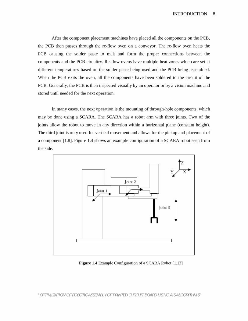
In many cases, the next operation is the mounting of through-hole components, which
may be done using a SCARA. The SCARA has a robot arm with three joints. Two of the
joints allow the robot to move in any direction within a horizontal plane (constant height).
The third joint is only used for vertical movement and allows for the pickup and placement of
a component [1.8]. Figure 1.4 shows an example configuration of a SCARA robot seen from
the side.
Figure 1.4 Example Configuration of a SCARA Robot [1.13]

“OPTIMIZATION OF ROBOTIC ASSEMBLY OF PRINTED CURCUIT BOARD USING AIS ALGORITHMS”
9 INTRODUCTION
After passing through these processes, the assembly of the PCB is complete. The PCB
may proceed to a testing operation before being assembled into the final electronic product.
The focus of this research is on the Chip Shooter machine, with emphasis on reducing the
placement time required to populate a PCB on the machine.
1.5 PCB Assembly Problem
PCB Assembly machines are facing mainly seven types of operational problems during
the process. These operational problems are closely related to two issues i.e. Setup
Management and Process Optimization [1.4]. Above decision problems are discussed below:
A. Processes Optimization:
o Component allocation: allocating component types to placement machines; o Feeder arrangement: assigning component types to feeders at each machine; o Component sequencing: determining the sequence of component Placements;
B. Setup Management:
o Machine grouping: grouping placement machines; o PCB sequencing: sequencing the production of PCBs; o PCB grouping: grouping PCBs into families; o Line assignment: assigning board types to assembly lines;
Among the above PCB assembly operations, the component sequencing is generally
the most time-absorbing operation [1.8] [1.9]. In addition, it is frequently a bottleneck in an
assembly line and determines the line cycle time [1.10]. Due to the large production volumes,
a minor reduction in cycle time will save significant production time. For example, to
produce 50,000 boards, a reduction of six seconds in cycle time will save 5,000 minutes, that
is, more than 80 working hours. Therefore, to increase the efficiency or minimize the cycle
time of the line, the component placement process must be optimized. Optimization of the
component placement process includes two interrelated problems: the component sequencing

“OPTIMIZATION OF ROBOTIC ASSEMBLY OF PRINTED CURCUIT BOARD USING AIS ALGORITHMS”
10 INTRODUCTION
problem and the feeder arrangement problem. So, the focus of this project work is mainly
confined to these two problems.
Generally, the component sequencing problem is alike to the travelling salesman
problem (TSP). This is the problem of finding the optimal placement order to visit a set of
components and return home with a minimum assembly distance or assembly time for the
PAP and the CS machines. On the other hand, the feeder arrangement problem is very like
the quadratic assignment problem (QAP). This is the problem of determining the optimal
arrangement to assign a set of component types to feeders with a minimum assembly distance
or assembly time for both types of machines.
For the PTH technology, the sequence of the insertion operation in the
autoinsertionmachine can be simply formulated as the TSP [1.11],and it is not necessary to
consider the feeder arrangement problem. However, inthe SMT environment, the efficiency
of the component placement process is alsodependent on a feeder to hold which types of
components besides the pick andplacement sequence. If the arrangement of components to
feeders is not donecarefully, even if the pick and placement sequencing is optimally solved, it
cancause significant deterioration in machines performance [1.12]. So, certainly, the
component sequencing problem as well as the feeder arrangementproblem should be solved
simultaneously.

”
Chapter 2
LITERATURE REVIEW

“OPTIMIZATION OF ROBOTIC ASSEMBLY OF PRINTED CURCUIT BOARD USING AIS ALGORITHMS”
12 LITRETUER REVIEW
2.1 Introduction
The literature related to the component placement sequence and feeder assignment problems
ispresented in this chapter. Although some researchers treat the problems independently,
thecomponent placement sequence and feeder assignment problems are highly related. The
firstsections of this chapter present the literature that addresses component sequencing
problem and the second section presents the literature that addresses both of these
problemstogether. Finally, a summary of the literature is presented.
2.2 Placement Sequencing Many authors have developed heuristics for solving the element placement sequence
problem.The question to be answered for this problem is: given a group of components with
their corresponding locations on the PCB, determine the component placement sequence that
minimizes the overall placement time.
Deo. et.al. [2.1] presented a multiple setup PCB assembly planning by genetic algorithm.
They developed GA program for optimize component sequencing problem of PCB assembly
with the help of a novel sequencing model for PCB and GA approach. Many researchers have
modelled the component placement sequencing problem for PCB assembly as a Travelling
Salesmen Problem (TSP) or a category of TSP [2.2] [2.3] [2.4]. The TSP is taken into
account a Non-Polynomial (NP) complete problem, therefore most researchers use heuristic
resolution approaches for finding sub optimal solutions within reasonable amounts of time.
Kho and Ong [2.5] imposed genetic algorithm to unravel the sequencing problem of PCB
assembly The approach takes into consideration component insertion priority and
sequencing decision rules[2.5]. A polygamy reproduction mechanism with dual mutation
has been proposed and implemented. They found that Performance analysis was carried out
using the PCB model adopted within the work of Sanchez and Priest. Preliminary
analysis shows that an improvement of 19.80% for the total distance travelled by the
machine bed was attainable. Further analysis reveals that there was space for still more
improvement.
Moyer and Gupta [2.6] address the component sequencing problem for a Chip Shooter
machine.This is one among of the few publications that provide a solution approach in which

“OPTIMIZATION OF ROBOTIC ASSEMBLY OF PRINTED CURCUIT BOARD USING AIS ALGORITHMS”
13 LITRETUER REVIEW
the component placement sequence for a Chip Shooter machine is optimized. Moyer and
Gupta present a close description of the Chip Shooter machine. The distance metric used for
the travelling distance between components is the Euclidean metric rather than the
Chebyshev metric (maximum of X and Y distance). They present the component sequencing
problem as a two-dimensional TSP and ignore the feeder assignment problem. The
assumption is that the PCB table movement time is generally more time consuming than the
feeder carriage movement time.Thus, minimizing the travelling distance between the
components on the PCB has a higher priority in their research.
The algorithm presented is a pair-wise exchange algorithm that requires as input an initial
placement sequence and the X-Y coordinates of the components on the PCB. Three
alternative methods for generating an initial placement sequence are described. These include
generating a component placement sequence based on a random selection, based on an
increasing component type identifier, and based on a sorting scheme of increasing X
coordinates, and subsequently the increasing Y coordinates of the components [2.14]. Moyer
and Gupta present an effective solution time saving methodology. When swapping two
components using the pair-wise exchange algorithm, the entire length of the placement
sequence is not re-calculated. Instead only the distance between the swapped components and
their immediate neighbours in the placement sequence is re-calculated to evaluate any
distance savings.
A real case study of a PCB containing 266 components is presented. The component
placement sequence for the 266 components is optimized by using the pair-wise exchange
algorithm. Three different initial placement sequences were used as input together with the
X-Y coordinates of the components. The shortest travelling distance was obtained when
using the initial placement sequence based on the component type identifier. The pair-wise
exchange heuristic improved the initial random solution by 81%, the initial solution based on
the component type identifier by 52%, and the initial solution based on sorting of the
components based on the X-Y coordinates by 64%. These results demonstrate that significant
improvements can be obtained by using a pair-wise exchange algorithm [2.15].
Other researchers such as Drezner and Nof [2.3], Ball and Magazine [2.2] and Donald and
Chan [2.4] have modelled the component sequencing problem for other types of placement
machines as a TSP or a class of TSP. Although the machine under study is the Chip Shooter

“OPTIMIZATION OF ROBOTIC ASSEMBLY OF PRINTED CURCUIT BOARD USING AIS ALGORITHMS”
14 LITRETUER REVIEW
machine, when ignoring the feeder carriage movement, the component sequencing problems
associated with the different types of placement machines become very similar.
Drezner and Nof [2.3] model the component sequencing problem for a pick and place
assembly robot as a TSP with predecessor constraints. The robot arm picks up components
from different bins and moves them to their corresponding assembly location. The
movements of the robot are divided into two categories: loaded arm movement and unloaded
arm movement. The loaded arm movements are fixed movements from the bins to the
assembly locations. Initially the locations of the bins are determined by solving the Bin
Assignment Problem (BAP) which minimizes the distance travelled between the bins and the
component assembly locations. The movement time of the unloaded arm is minimized by
solving the TSP with predecessor constraints heuristically. An example with numerical
results is presented, but no solution procedure steps are presented.
Ball and Magazine [2.2] modelled the component sequencing problem as a Rural Postman
Problem (RPP), which is an extension of the TSP. The machine described in this publication
is a gantry machine, which works with a stationary feeder carriage and has a pick and place
head. To solve the problem, a network of nodes is developed, where the nodes correspond to
the feeder slot locations and component locations. The possible movements between the
nodes are divided into two types: movements from feeder nodes to component nodes and
from component nodes to feeder nodes. The first type of movement is called “required”
because once the component types have been assigned to the feeder slots these movements
are fixed since the head must move from the feeder containing the component type to each
component location. The second type of movement is called “non-required” and depends on
the component placement sequence. After defining the network of possible nodes and the
types of possible movements, a closed path between the nodes that minimizes the distance
travelled by the placement head is found applying an Euler tour algorithm.
Donald and Chan [2.4] also formulate the component sequencing problem for a gantry
machine as a TSP. The machine analysed has an independent feeding mechanism that
provides the placement head with the components to be mounted. The machine consists of a
head that moves in the Z (vertical) direction and a PCB table that moves in the X-Y
directions. Donald and Chan [2.4] assume that the feeding mechanism movement time is
faster than the PCB table movement time; therefore the problem is modelled as a TSP

“OPTIMIZATION OF ROBOTIC ASSEMBLY OF PRINTED CURCUIT BOARD USING AIS ALGORITHMS”
15 LITRETUER REVIEW
governed by the PCB table movement. TRAVEL software, which uses a combination of 2-
optimal, 3-optimal and Lin-Kerninghan algorithms, was used to solve the TSP example
presented. A production case study was conducted with a single PCB type and an 8% saving
for overall processing time was obtained from a 43% reduction on PCB table movement time.
This shows that in many cases generating a component placement sequence based on
minimizing the PCB table movement can reduce the overall assembly time.
Because of the similarity between the TSP and the component sequencing problem given a
fixed feeder assignment, further literature review addressing the TSP is presented in this
section. Mandl [2.7], Smith [2.8] and Lawler et al. [2.9] present algorithms to solve the TSP.
The solution approach proposed by Mandl [2.7] is a branch and bound method that will not
be discussed any further due to its high solution time.
Smith [2.8] presents two solution approaches to the TSP. These include an approximate
method called the two optimal methods and an exact solution approach known as Little’s
algorithm. However, Little’s algorithm will not be discussed due to its large computational
time. The two optimal methods require as input an initial path between the locations of the
cities (components).
This initial path can be created using a construction heuristic such as the nearest neighbour
algorithm, which consists of choosing an initial city and then travelling from one city to the
next closest city until all the cities are included in the travelling path. Once an initial path
exists, the two optimal methods systematically swap two cities in the travelling sequence. If
the total travelling distance is reduced, then the swap is accepted and the swapping process is
repeated starting again from the first city in the travelling path. Otherwise, the swap is not
conducted and another interchange is proposed. This process is repeated until all possible
swaps of two cities are tried and no further reduction of the total travelling distance is
obtained.
Lawler et al. [2.9] presents several heuristics to solve the TSP. These heuristics include the,
furthest insertion point, nearest neighbour algorithm, arbitrary insertion point, two optimal,
three optimal, and or-optimal. The authors describe each of the heuristics briefly and compare
the quality of their solutions.

“OPTIMIZATION OF ROBOTIC ASSEMBLY OF PRINTED CURCUIT BOARD USING AIS ALGORITHMS”
16 LITRETUER REVIEW
The nearest neighbour algorithm, furthest insertion point, and arbitrary insertion point are
construction heuristics. The nearest neighbour algorithm consists of choosing an initial
starting point or city and then travelling to the nearest city until all cities are included in the
path. The furthest insertion point consists of choosing a starting city and then adding to the
tour the city located the furthest away. Once two cities are in the tour, the next city chosen is
the one with the minimum furthest distance away from each of the cities in the tour. The
chosen city is then inserted in the tour between the two cities that minimize the increase in
the tour length. This procedure is repeated until all cities are assigned. The arbitrary insertion
point consists of choosing a starting city and then arbitrarily choosing another city to form an
initial tour. The length of the initial tour is calculated. Then another city is selected arbitrarily
and added to the initial tour in the position where the tour length increases the least. This
procedure is repeated until all the cities are included in the tour. Two optimal, three optimal
and or-optimal are improvement heuristics that require an initial tour. Given an initial tour the
two optimal and three optimal perform two and three city exchanges in the tour respectively.
If the tour length improves by exchanging the order of the cities in the tour, then the
exchanged is performed otherwise the exchange is not performed. This procedure is repeated
until no further reduction in the tour length is obtained. The or-optimal is a modified version
of the three optimal, which considers only a small percentage of exchanges that would be
considered by a regular three optimal. The or-optimal considers only those exchanges that
would result in a string of one, two, or three currently adjacent cities being inserted between
two other cities [2.15].
The tests show that for the construction heuristics, arbitrary insertion point outperforms the
furthest insertion point heuristic, and the furthest insertion point outperforms the nearest
neighbour heuristic. For the set of improvement heuristics two optimal outperforms the three
optimal when using equivalent run times, the or-optimal algorithm was not included in the
comparison.
Ayob and Kendell presents A survey of surface mount device placement machine
optimisation: Machine classification , they surveyed the characteristics of the various
machine technologies and classifies them into five categories (dual-delivery, multi-station,
turret-type, multi-head and sequential pick-and-place), based on their specifications and
operational methods.[2.10].Van Breedam [2.11], Otten and Van Ginneken [2.12], Press et al.
[2.13], and Golden and Skiscim [2.14] present the application of Simulated Annealing (SA)

“OPTIMIZATION OF ROBOTIC ASSEMBLY OF PRINTED CURCUIT BOARD USING AIS ALGORITHMS”
17 LITRETUER REVIEW
to the TSP. Although the algorithms they present vary slightly, they all work under the
concept of SA. SA consists of moving from an existing solution (a travelling path or
component placement sequence) to a proposed solution (another possible travelling path or
placement sequence) based on probability. The algorithm keeps track at all times of the best
solution found. When a solution is generated (using pair-wise exchange or other methods)
from the current solution, two possible cases exist. The first case is the case in which the
proposed solution is better than the current solution and the proposed solution (travelling path
or placement sequence) is accepted, thereby replacing the current solution. If the proposed
solution is also better than the best solution then the best solution is also replaced. The second
scenario is the one in which a worse solution than the current solution is found. For this case,
the Boltzmann density function is used to calculate the probability of accepting the proposed
solution to replace the current solution [2.12]. Boltzmann density function is a function of the
proposed solution objective function value (total travelling distance between cities or
components), the objective function values of the past solutions, and the annealing
temperature, which is a function of the number of iterations performed. The outcome of this
calculation is a number between zero and one, which is then compared to a randomly
generated number between zero and one. If the calculated number is less than or equal to the
randomly generated number, then the proposed solution is accepted and replaces the current
solution. Otherwise, the proposed solution is rejected. This process allows escaping from
local minimum solutions. As the number of iterations increases, the annealing temperature
decreases therefore decreasing the probability of accepting bad solutions or escaping from
local minimum, leading to a final solution where no improvements are found. Van Breedam
[2.11] obtained better results using SA to solve the TSP as compared to improvement
algorithms, which always end at the first local minimum.
Golden and Skiscim [2.14] applied SA combined with the two reverse algorithm to resolve
the TSP and compare their results to those obtained using different heuristics. The two
reverse algorithms are analogous to the two optimal algorithms. The underlying difference
between the two optimal and also the two reverse algorithm presented within this publication
is that in the two reverse algorithm only two arcs are modified within the route of the TSP.
This can be achieved by reversing the order of the cities in a portion of the travelling
salesman tour. In the regular two optimal four arcs are changed when the order of two cities
is swapped in the route. The two reverse procedure used to generate new solutions in the SA
routine, tends to generate solutions more similar to the current solution than with the two
“OPTIMIZATION OF ROBOTIC ASSEMBLY OF PRINTED CURCUIT BOARD USING AIS ALGORITHMS”
18 LITRETUER REVIEW
optimal since only two arcs are changed in the route instead of four. The SA used with the
two reverse to generate solutions is compared to the two reverse by itself and also to the
CCAO heuristic. The CCAO heuristic is a hybrid procedure that uses a starting sub tour of
cities and inserts cities to the sub tour using cheapest insertion criteria (least increase in
travelling distance). Then the initial solution is improved using a branch-exchange heuristic
and the or-optimal heuristic. The results show that the CCAO heuristic and the two reverse
algorithms by itself performed better than SA using the two reverse to generate new solutions
for the TSP.
2.3 Placement Sequencing and Feeder Assignment Several authors have also developed heuristics for solving the component sequencing
problem and the feeder assignment problem considering the inter relationship between them.
As mentioned previously, the placement time of a set of components is highly dependent on
both the placement sequence and the feeder assignment. In the previously described papers,
each of these problems has been addressed separately under the strong assumption that the
total placement time is mainly dependent on either the component sequencing or the feeder
assignment.
Although this assumption may hold valid for some of the placement machines, it generally
does not hold for the Chip Shooter machine since both the PCB table and the feeder carriage
can potentially delay the placement of a component.
McGinnis et al. [2.16] provide a formal description of the feeder assignment and placement
sequencing problem and describe the related literature. The authors emphasize the importance
of considering the relationship between the problems for concurrent type machines, such as
theChip Shooter machine.
This section presents the articles that have focused on solving both of these problems as
related problems. Some authors such as Gupta and Moyer [2.6], Leu et al. [2.17] and Kumar
and Li [2.18] have developed mathematical and heuristic approaches to solve these problems
On the other hand, De Souza and Lijun [2.19] and Huang et.al. [2.20] has developed
knowledge-based solution approaches.
Gupta and Moyer [2.6] present an efficient solution approach for determining the component
placement sequence and the feeder assignment for a Chip Shooter machine. The algorithm

“OPTIMIZATION OF ROBOTIC ASSEMBLY OF PRINTED CURCUIT BOARD USING AIS ALGORITHMS”
19 LITRETUER REVIEW
consists of a one-step iterative process between the component sequencing and the feeder
assignment problems. The algorithm starts by generating an initial placement sequence using
the nearest neighbour algorithm. The solution is improved using a pair-wise exchange until
all the possible pair-wise exchanges have been attempted or a pre specified maximum
numbers of non-improving solutions are reached. The solution approach keeps at all times a
list with a predetermined number of the best placement sequences obtained throughout the
improvement process. Once a final list of placement sequences has been generated, a feeder
routine, which m constructs and improves a feeder assignment for each of the placement
sequences, is used. The initial feeder assignment is constructed based on the component
indicator number, and although it provides an initial solution, this may not be the best way to
do it. The feeder assignment routine combines the initial feeder assignment data with the first
placement sequence on the list and the placement time is calculated. For each of the
placement sequences under study, a pair-wise exchange heuristic is applied to the initial
feeder assignment to improve the placement time. The feeder assignment pair-wise exchange
routine stops either when all the possible exchanges have been performed or a pre specified
numbers of non-improving solutions are reached. The feeder assignment routine is then
applied to the next placement sequence in the list. At the end of the process the placement
sequence and feeder assignment combination that yields the smallest placement time is
chosen as the final solution.
An important feature of the component sequencing routine is that when a proposed placement
sequence is worse than the best placement sequence by a pre specified percentage, the longest
link in the proposed component placement sequence is saved in tabu list so that it would not
be used in future solutions. The algorithm was tested against those proposed by Leu et al.
[2.17] and De Souza and Lijun [2.19]. The results of the algorithm proposed by Gupta and
Moyer [2.6] outperform both of these although they do not assume a cyclic system in which
the placement time of a component is dictated by the slowest of the three machine
mechanisms (turret head, PCB table and feeder carriage).
Leu et al. [2.17] presents a solution approach for the component sequencing problem and the
feeder assignment problem using genetic algorithms. They present genetic algorithms to
solve both of these problems for three different types of placements including the Chip
Shooter machine. The genetic operators used to create new solutions based on the parent
solutions include a modified crossover operator, mutation operator, inversion operator, and

“OPTIMIZATION OF ROBOTIC ASSEMBLY OF PRINTED CURCUIT BOARD USING AIS ALGORITHMS”
20 LITRETUER REVIEW
rotation operator. The algorithms allow setting of parameters that specify the number of
solutions to be created at each iteration using each of the genetic operators. Moreover, they
optimize both the placement sequence and feeder assignment simultaneously using two links:
one being the placement sequence and the other the feeder assignment. These two links are
then combined to calculate the overall placement time. The distance metric used for the
movement of the PCB table is the Chebyshev metric and for the feeder carriage movement
the Euclidean metric distance is used although the feeder carriage is supposed to move on a
single axis. The algorithm is tested with 50 components, assuming values for the PCB table
speed, the feeder carriage and the turret head rotation time. The results stated in the
publication appear inconsistent with the results shown in the plots and the placement path
shown.
Kumar and Li [2.18] formulate the placement sequencing problem and the feeder assignment
problem for an automated assembly machine consisting of a robotic arm, a stationary PCB
table, and a stationary feeder carriage as a combination of the TSP and the minimum weight
matching problem (MWMP). By decomposing the problem into a TSP assuming a feeder
assignment and a MWMP assuming a placement sequence they determine an upper bound.
Then they suggest finding lower bounds using relaxation techniques such as linear
programming relaxation or Lagrangian relaxation. The bonds are found in order to evaluate
any possible solutions. The authors present an experiment in which the placement sequence
and feeder assignment for ten different PCB configurations with 100 components are
optimized. They use a software package called SAS/OR to solve the MWMP in polynomial
time and use their own software (UK-TSP) which employs heuristics such as nearest
neighbour, nearest insertion, furthest insertion and random generation to generate an initial
placement sequence. The software then uses two optimal and three optimal to improve the
initial placement sequence. The results obtained are tested against those obtained by using the
S shape method and greedy algorithm. The proposed solution approach performed on average
24.11% and 25.35% better than the S shape method and the greedy algorithm respectively.
De Souza and Lijun [2.19] developed a knowledge-based system to address the component
sequencing and feeder assignment problems for the Chip Shooter machine. The components
are separated into different groups based on the component size and quantity. Then the
arrangement of the feeders is conducted based on the component size groups and the location
of the components on the PCB. A TSP module is then used to determine the placement

“OPTIMIZATION OF ROBOTIC ASSEMBLY OF PRINTED CURCUIT BOARD USING AIS ALGORITHMS”
21 LITRETUER REVIEW
sequence of two, three or even more type components from the same group. The TSP module
uses a minimum spanning tree (MST) combined with a knowledge-based heuristic that yields
results of guaranteed worst-case performance. An example is presented in which the
placement sequence and feeder assignment for a PCB with 14 components is optimized. The
results obtained are compared to those obtained using the heuristic in the multi-head
concurrent operation (MCO) placement machine. The MCO heuristic gives a total placement
time of 5.67 seconds versus 4.10 seconds when using the knowledge-based system. However,
no clear conclusions regarding the performance of the knowledge base solution approach can
be made from an experiment with only one replication.
Huang et al. [2.20] also focus their efforts on developing a knowledge-based system to solve
the component sequencing problem and the feeder assignment problem for multiple batches
of PCBs. The machine under study is the gantry machine with two mounting heads, a moving
PCB table, and stationary feeder carriages. The expert system generates a feeder assignment
in which the component types that are mounted with the highest frequency are assigned to the
feeder slots that are the closest to the PCB table. Once the feeders have been assigned to the
feeder slots using the feeder location arrangement module of the knowledge-based system,
the tooling and nozzle calculation module generate alternative placement sequences using a
hill-climbing algorithm, which requires short computation time. This generates placement
sequences that minimize the nozzle changes and possible contingencies between the two
heads. The travelling path evaluation module then evaluates the component placement
sequences and the best sequence is selected. The main advantage of the expert system is that
it takes into account the possible constraints that are encountered in the assembly of PCBs
and relaxes many of the assumptions made by other authors.
2.4 Summary of Literature Review
The literature reviewed in this chapter described the component sequencing problem
individually and as inter related with feeder assignment problems for different types of
placement machines. Because of the similarity between these two problems and the TSP and
QAP respectively, publications dealing with the TSP and QAP were also described.
The publications dealing with the component sequencing problem and the feeder assignment
problem provided construction heuristics such as nearest neighbour, furthest insertion point,

“OPTIMIZATION OF ROBOTIC ASSEMBLY OF PRINTED CURCUIT BOARD USING AIS ALGORITHMS”
22 LITRETUER REVIEW
arbitrary insertion point, greedy algorithm, etc. Most publications also propose improvement
heuristics such as pair-wise exchange, two optimal, three optimal and some variation of tabu
search to improve upon the initial solutions obtained using the construction heuristics. One of
the publications proposed genetic algorithms as a solution approach. All of these solution
approaches iterate searching for a better solution as long as improvements can be achieved
and better solutions can be obtained. However, the publications that specifically addressed
the component sequencing problem and the feeder assignment problem for the Chip Shooter
machines did not take into account some important characteristics of the assembly process.
PCB table is not constant, but instead it is a function of the distance travelled and the type of
components mounted on the PCB. Not all component feeders occupy a single feeder slot, but
may occupy more than one feeder slot because of the size of the component. This adds
additional travel distance and capacity requirements on the feeder carriage mechanism. All of
the publications assumed that the PCB table velocity and the feeder carriage velocity are
constant when they are not. Assuming a constant velocity for these mechanisms provides a
misleading placement time estimate, which in many cases is used as the performance measure
of the solution approaches described in the publications reviewed.
This research will focus on developing a solution approach for the component sequencing
problem with fix feeder arrangement for the Pick and Place machine using construction and
improvement Artificial immune system algorithm. Furthermore, the proposed solution
approach will relax the assumptions previously mentioned.

Chapter 3
TECHNIQUES FOR OPTIMIZATION OF PCB ASSEMBLY

“OPTIMIZATION OF ROBOTIC ASSEMBLY OF PRINTED CURCUIT BOARD USING AIS ALGORITHMS”
24 TECHNIQUES FOR OPTIMIZATION OF PCB ASSEMBLY
3.1 Introduction
Assembly of printed circuit board is a based on the principle of Travel Salesman Problem
(TSP). The Travelling Salesman Problem or the TSP is a representative of a large class of
problems known as combinatorial optimization problems. In the ordinary form of the TSP, a
map of cities is given to the salesman and he has to visit all the cities only once to complete a
tour such that the length of the tour is the shortest among all possible tours for this map.In
general, the TSP includes two different kinds, the Symmetric TSP and the Asymmetric TSP
[3.1]. In the symmetric form known as STSP there is only one way between two adjacent
cities, i.e., the distance between cities A and B is equal to the distance between cities B and A
(Fig. 3.1). But in the ATSP (Asymmetric TSP) there is not such symmetry and it is possible
to have two different costs or distances between two cities. Hence, the number of tours in the
ATSP and STSP on n vertices (cities) is (n-1)! and (n-1)!/2, respectively
Fig. 3.1 The tour with A=>B =>C =>E =>D => A is the optimal tour [3.1]
There are different approaches for solving the TSP. Solving the TSP was an interesting
problem during recent decades. Almost every new approach for solving engineering and
optimization problems has been tested on the TSP as a general test bench. First steps in
solving the TSP were classical methods. These methods consist of heuristic and exact
methods. Heuristic methods like cutting planes and branch and bound [3.2], can only
optimally solve small problems whereas the heuristic methods, such as 2-opt [3.3], 3-opt,
Markov chain [3.4] simulated annealing [3.5] and tabu search are good for large problems.
Besides, some algorithms based on greedy principles such as nearest neighbour, and spanning

“OPTIMIZATION OF ROBOTIC ASSEMBLY OF PRINTED CURCUIT BOARD USING AIS ALGORITHMS”
25 TECHNIQUES FOR OPTIMIZATION OF PCB ASSEMBLY
tree can be introduced as efficient solving methods. Nevertheless, classical methods for
solving the TSP usually result in exponential computational complexities. Hence, new
methods are required to overcome this shortcoming. These methods include different kinds of
optimization techniques, nature based optimization algorithms, population based optimization
algorithms and etc. In this chapter we discuss some of these techniques which are algorithms
based on population.
Population based optimization algorithms are the techniques which are in the set of the nature
based optimization algorithms. The creatures and natural systems which are working and
developing in nature are one of the interesting and valuable sources of inspiration for
designing and inventing new systems and algorithms in different fields of science and
technology. Evolutionary Computation [3.6], Neural Networks [3.7], Time Adaptive Self-
Organizing Maps [3.8], Ant Systems [3.9], Particle Swarm Optimization [3.10], Simulated
Annealing [3.11], Bee Colony Optimization [3.12] and DNA Computing [3.13] are among
the problem solving techniques inspired from observing nature.
In this chapter population based optimization algorithms have been introduced. Some of these
algorithms were mentioned above. Other algorithms are Intelligent Water Drops (IWD)
algorithm [3.8], Artificial Immune Systems (AIS) [3.14] and Electromagnetism-like
Mechanisms (EM) [3.15]. In this chapter, every section briefly introduces one of these
population based optimization algorithms used for solving the TSP in past researches.
3.2. Evolutionary algorithms
3.2.1 Introduction:
Evolutionary Algorithms (EAs) imitates the process of biological evolution in nature. These
are search methods which take their inspiration from natural selection and survival of the
fittest as exist in the biological world. EA conducts a search using a population of solutions.
Each iteration of an EA involves a competitive selection among all solutions in thepopulation
which results in survival of the fittest and deletion of the poor solutions from the population.
By swapping parts of a solution with another one, recombination is performed and forms the
new solution that it may be better than the previous ones. Also, a solution can be mutated by
manipulating a part of it. Recombination and mutation are used to evolve the population
towards regions of the space which good solutions may reside.
“OPTIMIZATION OF ROBOTIC ASSEMBLY OF PRINTED CURCUIT BOARD USING AIS ALGORITHMS”
26 TECHNIQUES FOR OPTIMIZATION OF PCB ASSEMBLY
Four major evolutionary algorithm paradigms have been introduced during the last 50 years:
genetic algorithm is a computational method, mainly proposed by Holland [3.15].
Evolutionary strategies developed by Rechenberg [3.16] and Schwefel [3.17]. Evolutionary
programming introduced by Fogel [3.18], and finally we can mention genetic programming
which proposed by Koza [3.19]. Here we introduce the GA (Genetic Algorithm) for solving
the TSP. At the first, we prepare a brief background on the GA.
3.2.2 Genetic algorithms:
Genetic Algorithms focus on optimizing general combinatorial problems. GAs have long
been studied as problem solving tools for many search and optimization problems,
specifically those that are inherent in NP-Complete problems. Various candidate solutions are
considered during the search procedure in the system, and the population evolves until a
candidate solution satisfies the predefined criteria. In most GAs, a candidate solution, called
an individual, is represented by a binary string [3.20] i.e. a string of 0 or 1 elements. Each
solution (individual) is represented as a sequence (chromosome) of elements (genes) and is
assigned a fitness value based on the value given by an evaluation function. The fitness value
measures how close the individual is to the optimum solution. A set of individuals constitutes
a population that evolves from one generation to the next through the creation of new
individuals and deletion of some old ones. The process starts with an initial population
created in some way, e.g. through a random process. Evolution can take two forms:
Crossover: Two selected chromosomes can be combined by a crossover operator, the result
of which will replace the lowest fitness chromosome in the population. Selection of each
chromosome is performed by an algorithm to ensure that the selection probability is
proportional to the fitness of the chromosome. A new chromosome has the chance to be
better than the replaced one. The process is oriented towards the sub-regions of the search
space, where an optimal solution is supposed to exist [3.20].
Mutation: In mutation process, a gene from a selected chromosome is randomly changed.
This provides additional chances of entering unexplored sub-regions. Finally, the evolution is
stopped when either the goal is reached or a maximum CPU time has been spent [3.20].
In the following the GA operation pseudo code has been written:
1. Start
“OPTIMIZATION OF ROBOTIC ASSEMBLY OF PRINTED CURCUIT BOARD USING AIS ALGORITHMS”
27 TECHNIQUES FOR OPTIMIZATION OF PCB ASSEMBLY
2. Population initialization
3. Repeat until (satisfying termination criteria)
• Selection
• Cross over
• Mutation
• Making new population with the fittest solutions
• Evaluation
• Checking the termination criterion
4. Take the best solution as output
5. End
3.3 Ant colony optimization (ACO)
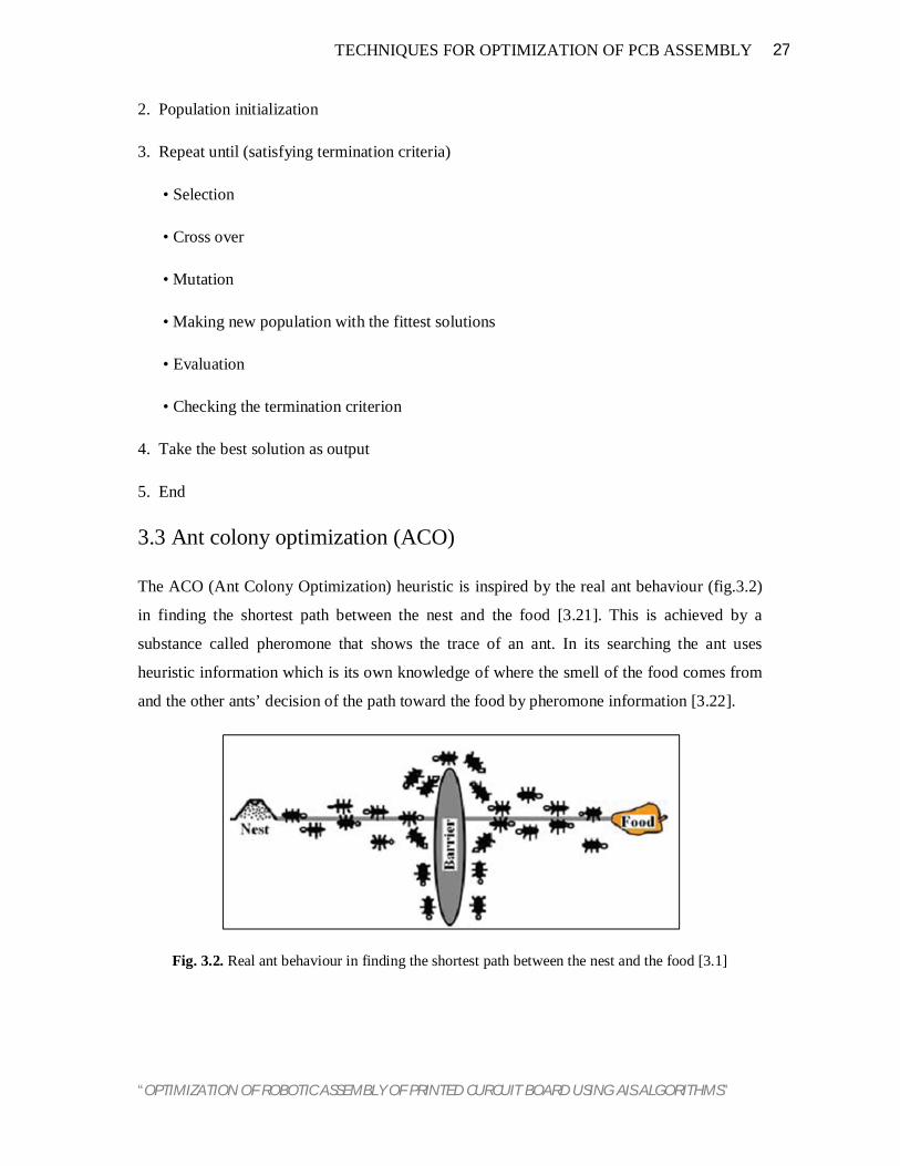
The ACO (Ant Colony Optimization) heuristic is inspired by the real ant behaviour (fig.3.2)
in finding the shortest path between the nest and the food [3.21]. This is achieved by a
substance called pheromone that shows the trace of an ant. In its searching the ant uses
heuristic information which is its own knowledge of where the smell of the food comes from
and the other ants’ decision of the path toward the food by pheromone information [3.22].
Fig. 3.2. Real ant behaviour in finding the shortest path between the nest and the food [3.1]

“OPTIMIZATION OF ROBOTIC ASSEMBLY OF PRINTED CURCUIT BOARD USING AIS ALGORITHMS”
28 TECHNIQUES FOR OPTIMIZATION OF PCB ASSEMBLY
In fact the algorithm uses a set of artificial ants (individuals) which cooperate to the solution
of a problem by exchanging information via pheromone deposited on graph edges. The ACO
algorithm is employed to imitate the behaviour of real ants and is as follows:
3.4 Particle swarm optimization (PSO)
Particle Swarm Optimization (PSO) uses swarming behaviors observed in flocks of
birds,schools of fish, or swarms of bees (figure 3.3), and even human social behavior, from
whichintelligence emerges [3.23].The standard PSO model consists of a swarm of particles.
They move iteratively through the feasible problem space to find the new solutions. Each
particle has a position represented bya position-vector 푥⃗(i is the index of the particle), and a
velocity represented by a velocity-vector푣⃗. Each particle remembers its own best position so
far in a vector 푥#⃗ and its j-th dimensional value is푥 #⃗ . The best position-vector among the
swarm heretofore is thenstored in a vector x* and its j-th dimension value is x*j .The PSO
procedure is as follows:
Initialize
Loop
Each ant is positions on a starting node.
Loop
Each ant applies a state transition rule to
incrementally build a solution and a local
pheromone updating rule.
Until all ants have built a complete solution.
A global pheromone updating rule is applied.
Until end condition

“OPTIMIZATION OF ROBOTIC ASSEMBLY OF PRINTED CURCUIT BOARD USING AIS ALGORITHMS”
29 TECHNIQUES FOR OPTIMIZATION OF PCB ASSEMBLY
Fig.3.3. Birds or fish exhibit such a coordinated collective behavior [3.1]
Algorithm 1 Particle Swarm Algorithm
01. Begin
02. Parameter settings and swarm initialization
03. Evaluation
03. g= 1
05. While (the stopping criterion is not met) do
06. for each particle
07. Update velocity
08. Update position and local best position
09. Evaluation
10. EndFor
11. Update leader (global best particle)
12. g+ +
15. End While
13. End
The PSO algorithm has several phases consist of Initialization, Evaluation, and Update
Velocityand Update Position.

“OPTIMIZATION OF ROBOTIC ASSEMBLY OF PRINTED CURCUIT BOARD USING AIS ALGORITHMS”
30 TECHNIQUES FOR OPTIMIZATION OF PCB ASSEMBLY
3.5 Intelligent water drops 3.5.1 Introduction The last work on the population based optimization algorithms inspired by nature is a
novelproblem solving method proposed by Hamed Shah-hosseini [3.7]. Thismethod is called
“Intelligent Water Drops” or IWD algorithm which is based on theprocesses that happen in
the natural river systems and the actions and reactions that takeplace between water drops in
the river and the changes that happen in the environment thatriver is flowing. Here we
prepare a complete description on this new and interestingmethod. To start with, the
inspiration of IWD, natural water drops, will be stated. After thatthe IWD system has been
introduced. And finally these ideas are embedded into theproposed algorithm for solving the
Traveling Salesman Problem or the TSP.
3.5.2 Natural water drops In nature, we often see water drops moving in rivers, lakes, and seas. As water drops
move,they change their environment in which they are flowing. Moreover, the environment
itselfhas substantial effects on the paths that the water drops follow. Consider a
hypotheticalriver in which water is flowing and moving from high terrain to lower terrain and
finallyjoins a lake or sea. The paths that the river follows, based on our observation in nature,
areoften full of twists and turns. We also know that the water drops have no visible eyes to
beable to find the destination (lake or river). If we put ourselves in place of a water drop of
theriver, we feel that some force pulls us toward itself (gravity). This gravitational force as
weknow from physics is straight toward the center of the earth. Therefore with no
obstaclesand barriers, the water drops would follow a straight path toward the destination,
which isthe shortest path from the source to the destination. However, due to different kinds
ofobstacles in the way of this ideal path, the real path will have to be different from the
idealpath and we often see lots of twists and turns in a river path. In contrast, the water
dropsalways try to change the real path to make it a better path in order to approach the
idealpath. This continuous effort changes the path of the river as time passes by. One feature
of awater drop is the velocity that it flows which enables the water drop to transfer an
amountof soil from one place to another place in the front. This soil is usually transferred
from fastparts of the path to the slow parts. As the fast parts get deeper by being removed
from soil,they can hold more volume of water and thus may attract more water. The removed
soilswhich are carried in the water drops are unloaded in slower beds of the river. There

“OPTIMIZATION OF ROBOTIC ASSEMBLY OF PRINTED CURCUIT BOARD USING AIS ALGORITHMS”
31 TECHNIQUES FOR OPTIMIZATION OF PCB ASSEMBLY
areother mechanisms which are involved in the river system which we don’t intend to
considerthem all here.
In summary, a water drop in a river has a non-zero velocity. It often carries an amount
ofsoil. It can load some soil from an area of the river bed, often from fast flowing areas
andunload them in slower areas of the river bed. Obviously, a water drop prefers an easier
pathto a harder path when it has to choose between several branches that exist in the path
fromthe source to the destination.
3.5.3 Intelligent water drops Based on the observation on the behavior of water drops, we develop an artificial waterdrop
which possesses some of the remarkable properties of the natural water drop. ThisIntelligent
Water Drop, IWD for short, has two important properties:
1. The amount of the soil it carries now, Soil (IWD).
2. The velocity that it is moving now, Velocity (IWD).
This environment depends on the problem at hand. In anenvironment, there are usually lots
of paths from a given source to a desired destination,which the position of the destination
may be known or unknown. If we know the position ofthe destination, the goal is to find the
best (often the shortest) path from the source to thedestination. In some cases, in which the
destination is unknown, the goal is to find theoptimum destination in terms of cost or any
suitable measure for the problem.
We consider an IWD moving in discrete finite length steps. From its current location
to itsnext location, the IWD velocity is increased by the amount nonlinearly proportional to
theinverse of the soil between the two locations. Moreover, the IWD’s soil is increased
byremoving some soil of the path joining the two locations. The amount of soil added to
theIWD is inversely (and nonlinearly) proportional to the time needed for the IWD to pass
fromits current location to the next location. This duration of time is calculated by the
simplelaws of physics for linear motion. Thus, the time taken is proportional to the velocity
of theIWD and inversely proportional to the distance between the two locations.
Another mechanism that exists in the behavior of an IWD is that it prefers the paths
withlow soils on its beds to the paths with higher soils on its beds. To implement this
behavior ofpath choosing, we use a uniform random distribution among the soils of the
available pathssuch that the probability of the next path to choose is inversely proportional to

“OPTIMIZATION OF ROBOTIC ASSEMBLY OF PRINTED CURCUIT BOARD USING AIS ALGORITHMS”
32 TECHNIQUES FOR OPTIMIZATION OF PCB ASSEMBLY
the soils ofthe available paths. The lower the soil of the path, the more chance it has for being
selected by the IWD.
In this part, we specifically express the steps for solving the TSP. The first step is how
torepresent the TSP in a suitable way for the IWD. For the TSP, the cities are often modeled
bynodes of a graph, and the links in the graph represent the paths joining each two cities.
Eachlink or path has an amount of soil. An IWD can travel between cities through these links
andcan change the amount of their soils. Therefore, each city in the TSP is denoted by a node
inthe graph which holds the physical position of each city in terms of its two
dimensionalcoordinates while the links of the graph denote the paths between cities. To
implement theconstraint that each IWD never visits a city twice, we consider a visited city list
for the IWDwhich this list includes the cities visited so far by the IWD. So, the possible cities
for an IWDto choose in its next step must not be from the cities in the visited list.
3.6 Bee colony optimization 3.6.1 Introduction Similar to other natural inspired and collective intelligence based algorithms such as
PSOwhich is taken from the bird’s life and ACO based on the ant colony social life, another
kindof artificial intelligence systems that can be useful in solving many
engineering,management, control and computational problems, is an algorithm inspired from
Beecolonies in nature. The Bee Colony Optimization (BCO) algorithms are interesting meta-
heuristic algorithms that represent another direction in the field of swarm intelligence.Here,
firstly we introduce the bee system and bee colony optimization briefly and then somerecent
works on the TSP which have used bee systems are investigated.
3.6.2 Bee colony optimization The bee colony’s function according to nature is as follows. At first, each bee belonging to
acolony looks for the feed individually. When a bee finds the feed, it informs other bees by
dancing. Other bees collect and carry the feed to the hive. After relinquishing the feed to
thehive, the bee can take three different actions.
1. Abandon the previous food source and become again uncommitted follower.
2. Continue to forage at the food source without recruiting the nest-mates.
3. Dance and thus recruit the nest-mates before the return to the food source.

“OPTIMIZATION OF ROBOTIC ASSEMBLY OF PRINTED CURCUIT BOARD USING AIS ALGORITHMS”
33 TECHNIQUES FOR OPTIMIZATION OF PCB ASSEMBLY
With a certain probability that is dependent on the obtained feed quality, its distance
fromthe hive and the number of the bees which are now engaged with this feed resource, a
bee selects one of the stated actions and follows its work in a similar repetitive form [3.24].
This behavior can be applied to many complicated engineeringproblems including
computational, control, optimization, transportation, etc. In thefollowing we study such a
method that focuses on the TSP solving.
3.6.3 BCO application The BCO algorithm can be a significant method in local search applications. One of the
mostprimary works on the bees and their life is [3.25]. In this study, the authorsapplied bee
system along with GA and introduced a modified and improved form of theconventional GA.
Based on this fact that the regular GA lacks the global search ability; theimprovement is
regarding to overcome this shortcoming. Hence, a new GA inspired by thebee colony’s
function has been presented, the authors called it, bee system. The mainpurpose of this
modified GA (bee system) is to improve the local search ability of Gaswithout degrading the
global search ability. In the proposed bee system, firstly global searchis performed using the
simple GA structure. Through this global search step, somechromosomes with reasonable
high fitness produced which are called superiorchromosome. These superior chromosomes
are kept for the local search procedure and eachof them corresponds to a local population. At
the beginning of the local search all of thechromosomes in each local population make couple
(crossover) with its population superiorchromosome. This crossover is named concentrated
crossover which tries to search concentratearound the related superior chromosome. Another
difference between thebee system and ordinary GA is migration among the population. In this
method, the beesystem selects one individual per predetermined generation, and transfers it to
the neighboring population which is called migration. All of the mentioned operators are in
the local searchpart. After passing the predetermined generations, the local search stops. If
the best solutionfound so far does not suffice the ending condition, the global search starts
again and the algorithm is repeated [3.25]
Chapter 4
THEORY OF ARTIFICIAL IMMUNE
SYSTEM

“OPTIMIZATION OF ROBOTIC ASSEMBLY OF PRINTED CURCUIT BOARD USING AIS ALGORITHMS”
34 THEORY OF ARTIFICIAL IMMUNE SYSTEM
4.1 Introduction
Recently, there was an increasing interest within the field of Artificial Immune
System (AIS) and its application for solving numerous issues specifically for the TSP [4.1],
[4.2]. AIS is impressed by natural immune mechanism and uses immunology method in
order to improve systems capable of performing variety of tasks in various areas of research
and analysissuch as diagnosis, pattern recognition, fault detection, and a number of other
research area as well asoptimization. Here we would like to know the AIS utterly. To begin
with, it would be helpful to become more acquainted with natural immune system.
Natural immune systems comprises the structures and processes within the living
body that offer a defence system against invaders and conjointly altered internal cells that
cause disease. During a glance, immune system’s main tasks are often divided into three
parts; recognition, categorization and defence. As recognition half, the immune system firstly
needs to identify the invader and foreign antigens e.g. bacteria, viruses and etc.
Oncerecognition part completes, classification should be performed by immune systems, this
is the second half. And acceptable kind of defence must to be applied for each class of
foreign aggressive phenomenon as the third half. The most important facet of the immune
systems in mammals is learning capability. Namely, the immune systems will grow
throughout the life time and is capable of using learning, memory and associative retrieval so
as to resolve mentioned recognition and classification tasks. Additionally, the studies show
that the natural immune systems are helpful mechanisms in data processing and might be
helpful in inspiration for problem solving and numerous optimization problems [4.3].
4.2 Artificial immune system
Like the natural immune systems the AIS is a group of techniques that attempt to
algorithmically mimic natural immune systems' behaviour [4.4]. As mentioned earlier, the
immune system is vulnerable to all of the invaders, additionally the outer influences, like
vaccines which are artificial ways of raising individual's immunity. Vaccines are other factors
that can stimulate the immune system’s susceptibility. This feature is the key point of the AIS
structure. The vaccines in the AIS are abstracted forms of the preceding information.
Vaccination modifies genes based on the useful knowledge of the problem to achieve higher
fitness in comparison to the fitness that obtained from a random process when for example a
classical GA is applied. Once again it is necessary to point out that, vaccines contain some
“OPTIMIZATION OF ROBOTIC ASSEMBLY OF PRINTED CURCUIT BOARD USING AIS ALGORITHMS”
35 THEORY OF ARTIFICIAL IMMUNE SYSTEM
important information about the problem and in consequence the vaccination process
employed in a right manner can be very useful in the performance of the algorithm. Like
classical GA and based on its structure the AIS can work. The GA operators (crossover and
mutation) search the problem space randomly and hence they don’t have enough capability of
meeting the actual problem at the local level. GAs are known as incapable of search fine local
tuning because they are global search algorithms. Immune method through vaccination tries
to overcome such blindness of crossover and mutation [4.3]. After vaccination, the immune
method might leads to deterioration. This case happens when vaccination leads to smaller
fitness values than previous ones. Hence, another important part of immune algorithm is
prevention of deterioration when inserting vaccine. In short, immune operators perform in
four steps: firstly, an individual is selected, randomly. Now as the second step, the vaccine is
inserted at the individual’s randomly chosen place. Vaccine insertion might leads to
deterioration, the third step is checking for deterioration. And finally the forth step is
discarding every individual that shows degeneration right after vaccine. This way of checking
could be dangerous for diversity and could result in algorithm's inability to avoid local
optima, especially when combined with small populations. The studies show that the use of
immune systems resulted in fasterconvergence when population is large enough and diversity
is secured. The combination of immune algorithm and GA, form the immune genetic
algorithm (IGA). Many of previous works that are performed on the TSP used IGA. Now, we
first investigate the IGA and its structure in detail and after that we have a look at some
previous works around the TSP [4.5].
In summary, the IGA consists of these steps:
1. Creation of initial population in some way, e.g. through a random process
2. Abstract vaccines according to the former information
3. Checking the termination criterion (if it is satisfied go to step 10 and else go to next step)
4. Crossover on the randomly selected individuals
5. Mutation on the produced children
6. Vaccination on the former step outcome
7. Deterioration checking

“OPTIMIZATION OF ROBOTIC ASSEMBLY OF PRINTED CURCUIT BOARD USING AIS ALGORITHMS”
36 THEORY OF ARTIFICIAL IMMUNE SYSTEM
8. Discarding every individual that shows degeneration right after vaccine
9. Go to step 3
10. End
As it is obvious from the ten steps which have been mentioned above, the IGA is very similar
to the conventional GA, but they are different in operators.
4.3 Theories of AIS The study and design of the artificial immune systems (AIS) is a relatively new area of
research that tries to build computational systems that are inspired by the natural biological
immune system. As we mentioned in subsection 3.3 there are many desirable computational
feature in BIS that can be used to solve computational problems. A typical AIS
model/algorithm implements one or more of these features. The books [4.4] and [4.6]
provides the detail of the modelling and applications of AIS. The four forms of AIS algorithm
reported in the literature are immune network model, negative selection, clonal selection and
danger theory.
4.3.1 Immune Network Model The immune network model was proposed by Jerne [4.7]. This theory proposed that the
immune system maintains aidiotypic network of interconnected cells for antigen recognition.
These cells both stimulate and suppress each other in a certain way that leads to stabilization
of network.
. Fig. 4.1 Presence of paratope and idiotope on antibody [4.5]

“OPTIMIZATION OF ROBOTIC ASSEMBLY OF PRINTED CURCUIT BOARD USING AIS ALGORITHMS”
37 THEORY OF ARTIFICIAL IMMUNE SYSTEM
The formation of such a network is possible by the presence of paratope and idiotope on the
each antibody cell. The paratope present on one B-cell is recognized by other B-cells
idiotopes so each cell recognizes as well as recognized. In this network two cells are
connected if the affinities they share exceed a certain threshold and the strength of the
connection is directly proportional to the affinity they share.
In network formation point of view two things are very important: antigen-antibody
binding and antibody-antibody binding. This idiotypic network can also be thought of as
having cognitive capabilities that makes it similar to a neural network [3.15].
4.3.2 Negative Selection Algorithm:
The purpose of negative selection is to provide tolerance for self-cells. It deals with the
immune system’s ability to detect unknown antigens while not reacting to the self-cells [4.8]-
[4.24]. During the generation of T-cells, receptors are made through a pseudo-random genetic
rearrangement process. Then, they undergo a censoring process in the thymus, called the
negative selection. There, T-cells that react against self-proteins are destroyed; thus, only
those that do not bind to self-proteins are allowed to leave the thymus. These matured T-cells
then circulate throughout the body to perform immunological functions and protect the body
against foreign antigens. This algorithm is given by Forest et al. [4.8], [4.9] whose main steps
are:
Step 1. In generation stage, the detectors are generated by some random process and
censored by trying to match self samples as shown in Fig 4.2(a).
Fig. 4.2(a) Censoring Stage. Fig.4.2(b) Monitoring Stage Fig. 4.2 Basic of Negative Selection Algorithm (a) Censoring Stage (b) Monitoring Stage [4.5]
“OPTIMIZATION OF ROBOTIC ASSEMBLY OF PRINTED CURCUIT BOARD USING AIS ALGORITHMS”
38 THEORY OF ARTIFICIAL IMMUNE SYSTEM
Step 2. Those candidates that match are eliminated and the rest are kept as detectors.
Step 3. In the detection stage, the collection of detectors (or detector set) is used to check
whether an incoming data instance is self or non-self as shown in Fig. 4.2(b).
Step 4. If it matches any detector, then it is claimed as non-self or anomaly.
4.3.3 Clonal Selection Algorithm The clonal selection principle of AIS describes how the immune cells eliminate a foreign
antigen and is simple but efficient approximation algorithm for achieving optimum solution.
The basic algorithm is first applied by Charsto et al. for solving optimization problems
[4.10]-[4.11]. The steps involved in the clonal selection algorithm are:
Step 1. Initialize a number of antibodies (immune cells) which represent initial population
size.
Step 2. When an antigen or pathogen invades the organism; a number of antibodies that
recognize these antigens survive. In Fig.4.3 only the antibody C is able to recognize
the antigen3 as its structure fits to a portion of the pathogen. So fitness of antibody C
is higher than others.
Step 3. The immune cells recognize antigens undergo cellular reproduction. During
reproduction the somatic cells reproduce in an asexual form, i.e. there is no crossover
of genetic material during cell mitosis. The new cells are copies (clones) of their
parents as shown for antibody C in Fig.4.3.
Step 4. A portion of cloned cells undergo a mutation mechanism which is known as somatic
hyper-mutation as described in [4.10].
Step 5. The affinity of every cell with each other is a measure of similarity between them. It
is calculated by the distance between the two cells. The antibodies present in a
memory response have on average a higher affinity than those of early primary
response. This phenomenon is referred to as maturation of immune response. During
the mutation process the fitness as well as the affinity of the antibodies gets changed.
In each iteration after cloning and mutation those antibodies which have higher fitness
and higher affinity are allowed to enter the pool of efficient cells. Those cells with
low affinity or self-reactive receptors must be efficiently eliminated.
Step 6. At each iteration among the efficient immune cells some become effecter cells
(Plasma Cell), while others are maintained as memory cells. The effecter cells secrete

“OPTIMIZATION OF ROBOTIC ASSEMBLY OF PRINTED CURCUIT BOARD USING AIS ALGORITHMS”
39 THEORY OF ARTIFICIAL IMMUNE SYSTEM
antibodies and memory cells having longer span of life so as to act faster or more
effectively in future when the organism is exposed to same or similar pathogen.
Step 7. The process continues till the termination condition is satisfied else steps 2 to 7 are
repeated.
Fig. 4.3 Basic of Clonal Selection Algorithm [4.5]
The clonal selection algorithm has several interesting features such as population size is
dynamically adjustable, exploration of the search space, location of multiple optima,
capability of maintaining local optima solutions and defined stopping criteria.
4.3.4 Danger Theory
This theory is given by Matzinger in 1994 [4.12]. The immune system in order to function
properly, it’s very important that only the “correct” cells are matched as otherwise this could
lead to a self-destructive autoimmune reaction. Classical immunology stipulates that an
immune response is triggered when the body encounters something non-self or foreign. It is
not yet fully understood how this self–nonself discrimination is achieved, but many
immunologists believe that the difference between them is learnt early in life. In particular, it
is thought that the maturation process plays an important role to achieve self-tolerance by
eliminating those T- and B-cells that react to self. In addition, a “confirmation” signal is
required: that is, for either B-cell or T- (killer) cell activation, a T- (helper) lymphocyte must

“OPTIMIZATION OF ROBOTIC ASSEMBLY OF PRINTED CURCUIT BOARD USING AIS ALGORITHMS”
40 THEORY OF ARTIFICIAL IMMUNE SYSTEM
also be activated. This dual activation is further protection against the chance of accidentally
reacting to self.
In accordance to danger theory there must be discrimination happening that goes
beyond the self–non-self distinction described above. For instance:
1. There is no immune reaction to foreign bacteria in the gut or to the food we eat although
both are foreign entities.
2. Conversely, some auto-reactive processes are useful, for example against self molecules
expressed by stressed cells.
3. The definition of self is problematic—realistically, self is confined to the subset actually
seen by the lymphocytes during maturation.
4. The human body changes over its lifetime and thus self changes as well. Therefore, the
question arises whether defences against non-self-learned early in life might be auto-reactive
later.
Other aspects that seem to be at odds with the traditional viewpoint are autoimmune diseases
and certain types of tumours that are fought by the immunesystem (both attacks against self)
and successful transplants (no attack against non-self). The Danger Theory takes care of
“non-self but harmless” and of “self but harmful” invaders into our system. The central idea
is that the immune system does not respond to non-self but to danger. Practically there is no
need to attack everything that is foreign, something that seems to be supported by the
counter-examples above. In this theory, danger is measured by damage to cells indicated by
distress signals that are sent out when cells die an unnatural death. As shown in Fig.4.4 a cell
that is in distress sends out an alarm signal, whereupon antigens in the neighbourhood are
captured by antigen-presenting cells such as macrophages, which then travel to the local
lymph node and present the antigens to lymphocytes [4.13]. Essentially, the danger signal
establishes a danger zone around itself. Thus B-cells producing antibodies that match
antigens within the danger zone get stimulated and undergo the clonal expansion process.
Those that do not match or are too far away do not get stimulated.

“OPTIMIZATION OF ROBOTIC ASSEMBLY OF PRINTED CURCUIT BOARD USING AIS ALGORITHMS”
41 THEORY OF ARTIFICIAL IMMUNE SYSTEM
Fig. 4.4 Principle of Danger Theory [4.5]
In accordance with Danger theory Bretscher and Chon proposed a two signal model.
According to this
Signal1: this is used for antigen recognition. Basically to determine the cell is a foreign cell.
Signal2: this is used for co-stimulation. This refers that the cell is really dangerous. So in
accordance to the two signal model the danger theory operates by 3 steps
Step 1. Become activated if you receive signals one and two together. Die if you receive
signal one in the absence of signal two. Ignore signal two without signal one.
Step 2. Accept signal two from antigen-presenting cells only. Signal one may come from any
cell.
Step 3. After activation revert to resting state after a short time.
The challenge is clearly to define a suitable danger signal. The danger signal helps to identify
which subset of feature vectors is of interest. A suitably defined danger signal overcomes
many of the limitations of self–non-self selection. It restricts the domain of non-self to a
manageable size, removes the need to screen against all self, and deals adaptively with
scenarios where self (or non-self) changes over time.

“OPTIMIZATION OF ROBOTIC ASSEMBLY OF PRINTED CURCUIT BOARD USING AIS ALGORITHMS”
42 THEORY OF ARTIFICIAL IMMUNE SYSTEM
4.4 Recent uses of AIS based Modelling
In recent years the area of Artificial Immune System (AIS) based modelling has drawn
attention of many researchers due to its broad applicability to different fields. Some of the
significant application areas include optimization problem [4.10]-[4.11], [4.14], computer
security [4.15], design of intrusion detection [4.16], fault detection [4.17], fault tolerance,
pattern recognition, distributed learning, sensor network, Job-shop scheduling, design of
recommendation system etc. The AIS is relatively young and emerging as an active and
attractive field involving models, techniques and applications of great diversity.
4.5 Summary
This chapter presents the functionality of BIS that is how the body restricts itself from the
invasion of external microorganisms. It also outlines how the artificial immune system (AIS)
is developed by following the principle of BIS. The four forms of AIS algorithm are
discussed and the application areas are highlighted. In the present the clonal selection
principle is chosen to be used for various applications as it is simple and easy to implement.
Chapter 5
PROBLEM DESCRIPTION

“OPTIMIZATION OF ROBOTIC ASSEMBLY OF PRINTED CURCUIT BOARD USING AIS ALGORITHMS”
45 PROBLEM DESCRIPTION
5.1 Types of PCB assembly used
Several researchers optimize the printed circuit board assembly problem by using different
type of assemblies. This is generally categorized on the basis of position of feeder available,
types of placement head, position of assembly board. Some of following are detailed below:
In a type-1 machine, a single feeder F1, possibly in the form of a magazine, provides
components to a single assembly head H (there is no turret) at a fixed location in the
horizontal X-Y plane. The head H also deposits components onto the PCB at a fixed point in
x-y. The table T moves in the X-Y plane so that components are placed at the desired
locations on the PCB. This type of assembly machine is the simplest and is normally adopted
when only one type of components has to be placed [5.1]. As shown in fig (5.1).
Fig 5.1 The assembly sequence of PCB with one set of feeder
In a type-2 machine, the two feeder (or feeder array) and the table are stationary (and
hence the PCB is also in a fixed location). The single assembly head H (again, there is no
turret) moves in the X-Y plane to carry components to the correct placement positions on the
PCB. If an array of feeders is adopted, the machine can be used to place components of
different types onto a PCB.As shown in fig (5.2).
3 2 1
(3) (2)
(2) (3) (1)
(2) (3) (1)
6
7
1
2
4 5
8
3
10
11
9
iii iv v
i ii
Starting point
Feeder number
Head movement sequence number
Component type
Component number

“OPTIMIZATION OF ROBOTIC ASSEMBLY OF PRINTED CURCUIT BOARD USING AIS ALGORITHMS”
46 PROBLEM DESCRIPTION
Fig.5.2 The assembly sequence of PCB with two set of feeder
Components are placed to correct placement positions on the PCB. If an array of feeders is
adopted, the machine can be used to place components of different types onto a PCB.
A type-3 machine has a turret carrying multiple pick-up/placement assembly heads H.
The centre of rotation of the turret is fixed in the X-Y plane. A feeder array F2 moves along
the X-axis to bring the feeder with the required component to the fixed pick- up location. The
table T moves in the X-Y plane to position different points of the PCB, in sequence, at the
fixed component placement location. Component pick-up and placement occur
simultaneously after the correct feeder and the table has reached their designated positions
and the turret has completed indexing the appropriate pick-up and placement heads. This type
of machine can also place components of different types. PCB assembly planning involves
two types of tasks: set-up management and process optimization. In the context of planning
for a single assembly machine with an array of feeders, set-up management can include
arranging the allocation of components among the different feeders or, alternatively, the
relative positioning of the feeders in the array, to help reduce assembly cycle times.
5
6 3
Starting point
4 3
12
(2) (1)
(3) (1)
(2) (2)
(2)
(3)
(1) (2)
1 7
2
3
4
5
6
8 9
10
11
13
1
2
Head movement sequence number
Component number
Component type
Feeder number

“OPTIMIZATION OF ROBOTIC ASSEMBLY OF PRINTED CURCUIT BOARD USING AIS ALGORITHMS”
47 PROBLEM DESCRIPTION
Process optimization for an assembly machine is usually a componentsequencing problem.
The aim of component placement sequencing is to optimize the movements of the table (in a
type-1 machine) or the assembly head (in a type-2 machine).as shown in fig.(5.3).
Fig.5.3 The assembly sequence of PCB with turret arrangement [5.1]
5.2 Proposed PCB assembly This work totally focuses on the sequential PAP machine. In this type of machines, the
components are stored in multiple stationary feeders. The placement head travels to pick up a
component from a feeder at a time, and then place it on the stationary board. The PAP
machine is able to achieve high accuracy, and suitable to operate with large components such
as integrated circuits (IC). The Operation sequence of PAP machine is that the placement
head starts from its original location (starting point or home position), moves to a feeder that
carries components, picks up a component from the feeder, and then moves to the desired
placement location on the stationary board, and places it there. After that, the head moves
back to the previous feeder if the next component is the same type with the previous one or
moves to another feeder to pick up the next component if it is different from the previous one
and place it on the board [5.2]. The head repeats this operation procedure until all
“OPTIMIZATION OF ROBOTIC ASSEMBLY OF PRINTED CURCUIT BOARD USING AIS ALGORITHMS”
48 PROBLEM DESCRIPTION
components are placed on the board and returns to its starting point, waits for the next board,
as illustrated in Fig. (5.4).
Consider a PCB to be assembled by a PAP machine. The PCB has 10 components with 6
different types. Each component type can be stored in any feeder, and a feeder can only store
a unique type of components, so 6 feeders are required. The objective of integrated problem
is to minimize the total travel distance of placement head, which includes the distance from
the starting point to a feeder at the beginning (i.e. d0f), the distances from a feeder to a
component’s position on the PCB (i.e., dfc), the distances from a component’s position to a
feeder (i.e., dcf), and the distance from the last component’s position to the starting point (i.e.,
di0). Suppose we have a sequence starting point-f3-c2-f3-c3-f2-c9-f2-c4-f1-c5-f1-c10-f6-c8-
f6-c7-f5-c6-f4-c1-starting point where f and c denotes feeder and component respectively. So
the sequence of component on PCB according to component number results as 2-3-9-4-5-10-
8-7-6-1, this sequence is called as antibody for artificial immune system and by using this
sequence, one can calculate the total travel distance of placement head by using the distance
calculating formula between two points i.e.
푑 , = (푥 − 푥 ) + (푦 − 푦 )
Here x1, y1are the coordinates of first point whereas x2, y2 are the coordinates of
second point and so on. The coordinates of all placement position on PCB and the
predetermined component arrangement in the feeders are tabulated in the Table. 1. The
coordinates are taken from the reference of starting point having coordinates (0, 0).
All the positions on PCB and feeders having a unique type of component are
predefined and fixed. We use above equation (1) to calculate all distance for example,
According to the above sequence, the head will move from starting point to the feeder 3, to
pick type 1component and then place this component on 2nd number of component on PCB
and coordinates according are (0, 0) , (10, 20) and (30, 30) respectively then the distance
travel by placement head to pick 1 type of component from starting point to the feeder 3 (i.e.
f3) is calculated as follows.
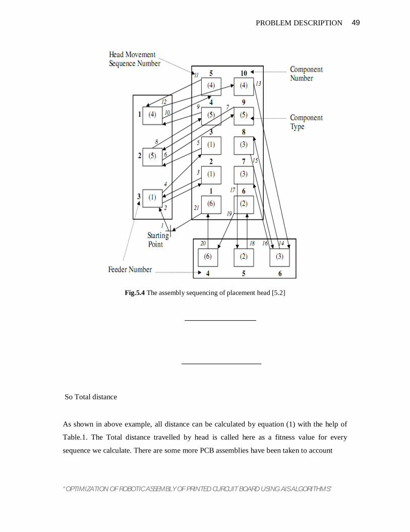
“OPTIMIZATION OF ROBOTIC ASSEMBLY OF PRINTED CURCUIT BOARD USING AIS ALGORITHMS”
49 PROBLEM DESCRIPTION
Fig.5.4 The assembly sequencing of placement head [5.2]
So Total distance
As shown in above example, all distance can be calculated by equation (1) with the help of
Table.1. The Total distance travelled by head is called here as a fitness value for every
sequence we calculate. There are some more PCB assemblies have been taken to account

“OPTIMIZATION OF ROBOTIC ASSEMBLY OF PRINTED CURCUIT BOARD USING AIS ALGORITHMS”
50 PROBLEM DESCRIPTION
Table.5.1Data of integrated problem with 10 components and 6 types [5.2]
component type Coordinates(mm) feeders Coordinates(mm)
x y x y
1 6 30 20 4 10 50
2 1 30 30 5 10 35
3 1 30 40 1 10 20
4 5 30 50 6 30 10
5 4 30 60 2 50 10
6 2 50 20 3 70 10
7 3 50 30
8 3 50 40
9 5 50 50
10 4 50 60
Table. 5.2 Component type and coordinates of different type of assembly problem [5.1][5.2]
Problem
type
component Type Coordinated(mm) feeders Coordinates (mm)
x y 4х2
problem
1 1 30 20 1 10 30
2 2 30 30 2 10 20
3 2 50 20
4 1 50 30
4х4
problem 1 4 30 40 1 10 30
2 3 30 60 2 10 20
3 1 50 60 3 20 10
4 2 50 40 4 30 10
6х4
problem 1 2 30 20 4 10 35
2 1 30 30 1 10 20
3 1 30 40 2 30 10
4 3 50 20 3 30 10
5 3 50 30
6 4 50 40

“OPTIMIZATION OF ROBOTIC ASSEMBLY OF PRINTED CURCUIT BOARD USING AIS ALGORITHMS”
51 PROBLEM DESCRIPTION
1 if component i is placed immediately before component j;
0 otherwise:
similar to above assembly 10х6 problem like 4х4, 4х2 and 6х4. The component arrangement
and the allocation of component on feeders and assembly are board tabulated in Table. 2
5.3 Mathematical Model As we already knows component sequencing and feeder arrangement problem are integrated
to each other without the solving one we cannot solve other problem so that for modelling of
mathematical model component sequencing problem, suppose the assignment of component
types to feeder is solved beforehand, the component sequencing model can then be
formulated for finding the optimal total travelling distance of placement head. In order to
achieve objective a decision variable has to be define as:
xij{
Actually, PAP component sequencing problem is totally based on TSP principle and
somewhat similarto the TSP also, except the objective function. For the PAP machine,
theobjective is not to minimize the distance between component iand component j because
the placement head is unable to placethe next component on the PCB immediately without
picking up acomponent from a feeder first. Therefore, the objective for thePAP machine
should be to minimize the summation of different distancesincluding [5.2]:
The distance between the position of component i on the PCB and feeder l (if i = 0, it
is the distance between the starting pointat the beginning and feeder l).
The distance between feeder l and the position of the next component.
The distance between the position of the last component i andthe starting point at the end.
The component sequencingproblem can be formulated as:
푚푖푛푖푚푖푧푒푑푖푠푡 = (푑 + 푑 ) + 푑 푥 (1)
Subjected to

“OPTIMIZATION OF ROBOTIC ASSEMBLY OF PRINTED CURCUIT BOARD USING AIS ALGORITHMS”
52 PROBLEM DESCRIPTION
푥 = 1푓표푟푗 = 0,1, … … ,푛; 푖 ≠ 푗.(2)
푥 = 1푓표푟푗 = 0,1, … … ,푛; 푗 ≠ 푖.(3)
푢 − 푢 + 푛푥 ≤ 푛 − 1푓표푟푖, 푗 = 0,1, … … , 푛; 푖 ≠ 푗.(4)
Equation (1) is an objective function which is formed to minimize the total travel distance
from placement head. If we assumed that PAP head is placing the components with constant
speed then the objective function will be change from travel distance to placement time for
assembling hole component on board. Equation (2) shows first set of constraint which ensure
that only one component must be placed immediately before jcomponent. Equation (3) shows
second set of constraint ensure that exactly one component must be place immediately after
icomponent. Above two constraint sets are not sufficient. Although the above two set of
constraint are satisfied by solution but solution may still be infeasible due to presence of sub-
tours. Therefor the third set of constraint added in above model, in order to remove sub-tours.
Due to the Placement head start assembly from starting point therefor it is redundant to
include i and/ or j = 0.
It is found form above model, objective function is a minimise type of non-linier integer
programming (NLP) model. It is very hard to solve by manually that is why we used one LP
commercial solver package LINGO to solve above NLP problem. This commercial package
gives an optimal solution which is compared with the global optimal solution got from the
artificial immune system algorithm.
5.4 Development of AIS algorithm
An evolutionary algorithm evolves its population in a way that makes individuals more and
more adapted to the environment. In other terms, the fitness function is minimized/
maximized. Real-life applications are of course much more complex, with the main problem
being to adapt, or even create operators that correspond to the problem at hand. The flow
chart of the AIS algorithm is shown in fig. 2. The operative mechanisms of immune system
are very efficient from a computational standpoint [5.3]. An AIS starts with an initial set of random solutioncalled population. Each solution in

“OPTIMIZATION OF ROBOTIC ASSEMBLY OF PRINTED CURCUIT BOARD USING AIS ALGORITHMS”
53 PROBLEM DESCRIPTION
population is called chromosome, which represent of point in the search space. The AIS
search process is one essential genetic operation: exploration (or diversification). Generally
the mutation operators explore the wide range of search space. The antibodies evolve
through successive iterations, called generations. During each generation the antibodies are
evaluated using some measures of fitness. The fitter the antibodies, the higher the
probabilities of being selected to perform a genetic operation (i.e. mutation). In the mutation
phase, the mutation operation maintains the diversity in population to avoid being trapped in
local optima. A new generation is formed by selecting some of the parents and offspring
according to their fitness value, and by rejecting others so to keep the population size
constant. After the predetermined number of generation is performed, the algorithm presents
the best antibodies, which hopefully present optimal solution or may be sub-optimal solution
to the problem [5.4].
As per as genetic algorithm AIS has also a great level of flexibility. It can be hybridized with
other heuristics in order to improve the solution further. The flowchart of AIS for the PAP
problem is shown in fig 5.5. The procedure of the AIS for PAP is listed as follows:
Step 1. Set the initial parameters like population size (pop), the number of iteration
(max_iter).
Step 2. Generate popinitial antibodies with one link encoding discussed in Section
5.3.1. For each chromosome, the link is generated by randomly generation.
Step 3. Evaluate the fitness value distas illustrated in section 5.3.2 for all antibodies in
the population.
Step 4. After the evaluation of dist, calculatethe affinity illustrated in section 5.3.3 for
all antibodies on the basis on which the cloning of antibodies will be carryout.
Step 5. Follow the selection procedure to select antibodies to perform the heuristic
mutation operation is section 5.3.4.
Step 6. Compare all clone with the antibodies in the population by the fitness value
dist. Retain the best pop antibodies in population.
Step 7. Population size after the mutation operations gone increased so that some
presents of population size are deleted any add new antibodies to achieve
predetermined population size called receptor editing described in section
5.3.5.
Step 8. Determine the best chromosome at each iteration. Repeat Step 3 to Step 8 until
max_iter iterations are performed.

“OPTIMIZATION OF ROBOTIC ASSEMBLY OF PRINTED CURCUIT BOARD USING AIS ALGORITHMS”
54 PROBLEM DESCRIPTION
Calculate sets of
Calculate Affinity
Clone the set of high Affinity sequence
Pair-wise Interchange Mutation
If Dist(new seq)<Dist(clone)
Inverse Mutation
Displacement Mutation
New sequence for next iteration
Clone=clone; sequence=clone
New sequence after Cloning and mutation
Receptor editing process
Clone=New sequence
Clone=New sequence
Clone=New sequence If Dist(new
seq)<Dist(clone)
If Dist(new seq)<Dist(clone)
Fig. 5.5 The Flow chart of artificial immune system algorithm for PCB assembly.

“OPTIMIZATION OF ROBOTIC ASSEMBLY OF PRINTED CURCUIT BOARD USING AIS ALGORITHMS”
55 PROBLEM DESCRIPTION
5.4.1 Encoding
An antibody is illustrated in Fig. (5.6) encoding of PCB and feeder representation, in which
the number inside the bracket in PCB represents the component type. For example, if the
sequence of placements starts with component 2, then component 3, component 9,
component 4, component 5, component 10, component 8, component 7, component 6 and
finally component 1. Its sequence can be represented as (2 3 9 4 5 10 8 7 6 1), that is, the
sequence of component on PCB, as shown in Fig. 5.6(a)
Fig. 5.6 (a) Encoding of given sequence of component is on PCB.
Fig 5.6(b) Encoding of feeder components.
If the ten components are from six component types, and type 4 is assigned to feeder 1,
whereas types 5, 1, 6, 2 and 3 are assigned to feeders 2, 3, 4, 5, 6 respectively, then the
feeder arrangement can be represented as (4 5 1 6 2 3). Sometimes, the number of feeders
available is more than that of component types required. Some components with the same
Component type
4 5 1 6 2 3
Feeder
1 2 3 4 5 6
1 2 3 4 5 6 7 8 9 10
Sequence
Component type
2(1) 3(1) 9(5) 4(5) 5(4) 10(4) 8(3) 7(3) 6(2) 1(6)
Component number

“OPTIMIZATION OF ROBOTIC ASSEMBLY OF PRINTED CURCUIT BOARD USING AIS ALGORITHMS”
56 PROBLEM DESCRIPTION
type can therefore be assigned to more than one feeder. Nevertheless, it was observed that no
more than two feeders with the same component type could be used on an assembly line.
Therefore, at most a particular component type can be stored in two feeders at the same time.
Not surprisingly, component types with greater use should have the priority to be assigned to
surplus feeders. In the above example, it is assumed that no one surplus feeder is available.
One type component is stored in only one of feeder. The feeder arrangement is now encoded
as (4 5 1 6 2 3), as illustrated in Fig. 5.6(b).
5.4.2 Evolution of fitness function
The fitness function used for PAP problem is total distance travelled by the placement head.
Fitness function calculates the total distance the head travelled. Its includes the distance from
original location i.e. starting point to a feeder at the beginning, the distance from a feeder to a
component on assembly board and the distance from last component to the original location.
Lets Dist(푥 ) be the fitness function for antibody 푥 in PAP problem, and D(a,b)represent the
distance between point a and b, then
퐷푖푠푡(푥 ) = 퐷 0, 푓(1) + 퐷(푓(푖), 푐 ) + 퐷(푐 ,푓(푖 + 1))
+ 퐷(푐 , 0)(5)
Where n is the number of component; f(i) is the feeder location for the ith component; ci is
the location of component at assembly board and 0 is the original location i.e. starting point.
Here, f(i)represent the feeder location for ith component. For example, for component 2, it is
stored in feeder 5, so f(2) = 5, that is f5 in the previous discussion.
5.4.3Clone Selection Principle
Each schedule (antibody) has a fitness value that refers to the affinity value of that antibody.
Affinity value of each schedule is calculated from the affinity function. The affinity function
is defined as:
퐴푓푓푖푛푖푡푦(푝) = 1
퐹푖푡푛푒푠푠푣푎푙푢푒(6)

“OPTIMIZATION OF ROBOTIC ASSEMBLY OF PRINTED CURCUIT BOARD USING AIS ALGORITHMS”
57 PROBLEM DESCRIPTION
From this relation, a lower fitness value gives a higher affinity value. Further the cloning of
antibodies is done directly proportional to their affinity function values. Therefore, there will
be more clones of antibodies that have lower fitness value than those with higher fitness
values in the new generated clone population. An immune based approach to minimize
fitness value on parallel processors has been presented in [5.5]. An affinity function is
defined based on fitness values of the schedules [5.6] [5.7] Also they have given a function to
calculate the number of clones that would be proliferated [5.8] [5.9].
5.4.4. Affinity mutation principles
The affinity maturation principle consists of three methods namely mutation and receptor
editing. Mutation a two phased mutation procedure which used for the generated clones [5.4].
a) Pair wise interchanges mutation.
b) Inverse mutation.
c) Displacement mutation.
5.3.4.(a) Pair wise Interchange Mutation:
Given a sequence s, let i and j be randomly selected two positions in the sequence s. A
neighbour of s is obtained by interchanging the jobs in positions i and j. If the fitness value of
the mutated sequence (after pair wise interchange mutation) is smaller than that of the
original sequence, then store the mutated one in the place of the original one, as shown in fig.
5.7.
Fig. 5.7The Pair wise interchange mutation operation.
5.3.4.(b) Inverse Mutation:
For a sequence s, let i and j be randomly selected two positions in the sequences. A neighbour
of s is obtained by inversing the sequence of jobs between i and j positions. If the fitness
value of the mutated sequence (after inverse mutation) is smaller than that of the original
sequence (a generated clone from an antibody), then the mutated one is stored in the place of
2 3 9 4 5 10 8 7 6 1
2 3 7 4 5 10 8 9 6 1
Parent:
Offspring1:

“OPTIMIZATION OF ROBOTIC ASSEMBLY OF PRINTED CURCUIT BOARD USING AIS ALGORITHMS”
58 PROBLEM DESCRIPTION
the original one. Otherwise, the sequence will be mutated again with random pair wise
interchange mutation. As shown in fig. 5.8.
Fig .5.8 The Inverse mutation operations.
5.3.4(c) Displacement Mutation:
In this method a sub tour is selected in random and it is removed from the tour and inserted it
in a randomly selected position. However the sub tour is inserted in reverse order as shown in
fig. 5.9.
Fig. 5.9 The Displacement mutation operation.
By using all above mutation techniques we got a very impressive and large variety of
antibodies in predefine population size.
5.4.5 Receptor Editing: After cloning and mutation processes, a percentage of the antibodies (worst %B of the whole
population) in the antibody population are eliminated and randomly created antibodies are
replaced with them. This mechanism allows finding new schedules that correspond to new
search regions in the total search space [5.10]. In this work, B is assumed as 30%, 50% and
80%.
2 3 7 8 5 4 9 10 6 1
2 3 9 4 5 10 8 7 6 1 Parent:
Offspring1:
Select sub-string
2 3 9 4 5 105
8 7 6 1
2 3 9 8 10 5 4 7 6 1
Flip the selected sub-string to for an offspring
Parent:
Offspring:

Chapter 6
RESULTS AND DISCUSSIONS
“OPTIMIZATION OF ROBOTIC ASSEMBLY OF PRINTED CURCUIT BOARD USING AIS ALGORITHMS”
60 RESULTS AND DISCUSSIONS
In this chapter the performance of AIS is evaluated by comparing to the optimal solution of
several problems mentioned in chapter 5. Here we have used two different type of
methodology to optimize the component sequencing problem i.e minimization of total
distance travelled by head of pick and place machine. First methodology based on the
specific AIS algorithm developed only for the PCB problem and second one based on the
Integer programming mathematical model. We have compared both of results obtained from
the above technics and also described the effect of AIS parameter on the solution obtained by
algorithm.
This part of the thesis is consist three part to evaluate the AIS algorithm’s performance. The
parts are as follows: First part consisting 10×6 PCB problem to evaluate the performance of
AIS algorithm and shows its characteristics in form of decrement graph. In second part, for
checking of homogeneity in solution we solved four different type of PCB assembly using
AIS and compared with the IP model. In third part the effect of receptor editing percentage
are shown during solving any problem from AIS algorithm.
6.1 Result of AIS performance At first to check the performance of AIS algorithm using a PCB assembly model which is
already discussed in chapter 5, it contains total 10 components on PCB assembly board
consist of 6 different type of components in different feeders so that here 6 numbers of
feeders are provided to pick the components and place it to their predefined position on the
assembly board with the help of PAP machine. Before starting the solution we have to decide
some AIS parameters like, population size (pop) = 20, number of iteration (max_itre) = 150,
receptor editing percentages (%B) = 50%, and perform the AIS algorithm. As a result of AIS
we obtained a global optimal point in the form of minimum travel distance by the PAP
machine is 575.3 cm in 30 iterations, the decrement graph between fitness value and number
of iteration is shown in fig 6.1.
6.2 Comparison with IP model For the checking of homogeneity of AIS algorithm we have taken some more problems to
solve them in AIS and integer programming methods. After iteration as we have received the
results of AIS is providing a very effective and efficient solution for every problem compared
to integer programming model. Here four types of problem are taken on which the AIS is

“OPTIMIZATION OF ROBOTIC ASSEMBLY OF PRINTED CURCUIT BOARD USING AIS ALGORITHMS”
61 RESULTS AND DISCUSSIONS
applied and the results are compared with the solution of integer programming mathematical
model. The comparison results of different problem using AIS and integer programming is
tabulated in Table 6.1. The problems are as follows:
Fig.6.1 Decrement graph between fitness value and iteration number.
1. 4х2 Problem: In this problem, a total of 4 components consisting of 2 different types
are considered. For these components two feeders are provided and each feeder
containing different type of component.
2. 4х4 Problem: In this problem, a total of 4 components consisting of 4 different types
are considered. For these components four feeders are provided and each feeder
containing different type of component.
3. 6х4 Problem: In this problem, a total of 6 components consisting of 4 different types
are considered. For these components four feeders are provided and each feeder
containing different type of component.
4. 10х6 Problem: In this problem, a total of 10 components consisting of 6 different
types are considered. For these components six feeders are provided and each feeder
containing different type of component.
570
580
590
600
610
620
630
640
0 5 10 15 20 25 30 35
Fitn
ess v
alue
( Dis
tanc
e in
cm
)
Number of Iterations
Series1

“OPTIMIZATION OF ROBOTIC ASSEMBLY OF PRINTED CURCUIT BOARD USING AIS ALGORITHMS”
62 RESULTS AND DISCUSSIONS
Table 6.1 Comparison table for different PCB problem
IP Model
Result
No. of
Iteration(IP
Model)
AIS
Result
No. of
Iteration
(AIS)
Percentages
of
effectiveness
4х2 Problem 267.69 16 236 12 11.8%
4х4 Problem 327.77 10 310 11 5.4%
6х4 Problem 320.17 18 312 14 2.5%
10х6
Problem
592.34 19 575.6 15 2.85%
6.3 Effect of receptor editing percentages In third part of result section we have been gone through the various effect on the total
distance travelled by the PAP head due to change in percentages of receptor editing. For this
part we have solved a 10×6 PCB assembly’s sequencing problem using AIS algorithm by
varying the receptor editing percentages in to three values i.e. 30%, 50% and 80%. The effect
on fitness value is plotted on graph. Shown in fig.6.2:
Fig.6.2 The effect of receptor editing percentage on fitness value.
570
580
590
600
610
620
630
640
0 10 20 30 40 50 60
Fitn
ess
valu
e (d
ista
nce
in c
m)
Number of iterations
30%
50%
80%

“OPTIMIZATION OF ROBOTIC ASSEMBLY OF PRINTED CURCUIT BOARD USING AIS ALGORITHMS”
63 RESULTS AND DISCUSSIONS
6.4 Discussion points As mentioned earlier, the fixed setup strategy is when part of the component types on a PCB
have already been assigned to the feeder carriage and the placement sequence are to be
determined. It means the component carrying by feeder is fixed or predefined; only
sequencing problem has been solved. When constructing a feederassignment for the
component types used on a PCB, the total number of component types alreadyassigned to the
feeder carriage consists of the component types of the PCBs whose feederassignment has
already been determined. The component types already assigned to the feedercarriage may or
may not include some of the component types used on the PCB whose feederassignment and
placement sequence is being constructed. So that in every type of PCBs problem used here to
solver using AIS have fixed feeders arrangement, they only used for optimize the minimum
travelled distance covered by PAP head to complete the whole assembly of PCB. After
evaluation of above results there are some points come in the picture for discussion. They are
listed below:
From fig. 6.1, AIS provide the global optimal value 575.3 in very small range of
iterations i.e. 30 only. Above AIS algorithm is only developed for the optimization of
sequencing problem.
The research carried out in this field reveals that very few researchers considered
sequencing problem in their work. Results are available for same type of PCB
assembly used above considering both problem feeder arrangement and component
sequencing. Due to this the result obtained by the researchers are quit less and
effective then the AIS results.
From Table 6.1, it shows that the AIS is providing an effective and efficient results in
very less number of iteration as compare to IP model which is solved by a commercial
IP solver “LINGO”.
From Fig. 6.2, it shows the effect of one of the parameter of AIS algorithm i.e.
Receptor editing percentages. Receptor editing is a kind of editing of worst antibodies
carryout within the algorithm after completing all type of mutation process during
transferring population size from current iteration to next iteration.
Variation in percentage of receptor editing shows that more % percentage receptor
editing provide more search space for optimization and take less number of iteration
to finding out the global optimal point.

Chapter 7
CONCLUSIONS AND FUTURE WORKS

“OPTIMIZATION OF ROBOTIC ASSEMBLY OF PRINTED CURCUIT BOARD USING AIS ALGORITHMS”
65 CONCLUSIONS AND FUTURE WORKS
7.1 Conclusions This research has addressed one of the decision problems associated with process
optimization in printed circuit board assembly systems for a specific assembly machine.
Specifically, a solution approach was developed for determining the component placement
sequence for a PAP style Chip Shooter type machine.An AIS algorithm has been proposed
for the pick and place sequence problem inPCB assembly, with the objective of minimizing
the PCBtotal assembly time. Results from this algorithm were subject to three segments:
Evolution of performance:For evolution of effectiveness, we assign a 10
component problem for checking the performance of AIS algorithm. We found that
it gives an optimal value which is very close to the result of researchers who found
out by considering feeder arrangement and component placement problem
together.
Comparison with IP model: the four different type of PCB assembly which
contains different number of component on the assembly board have used to
compare result of AIS with the mathematical tool i.e. IP model.The result shows
that AIS is providing a better global optimal solution in less number of iteration as
compare to the IP models results.
Effect of receptor editing percentage:To evaluate the effect of receptor editing
percentage, we have ranged the percentage in to three values i.e. 30%, 50% and
80%. We have found that the increase in receptor editing percentages also increase
the search space for optimization and decreases the number of iteration to obtain
the optimal point.
For a small problem, such as our 10 component example, the benefit of a better
solution may be small unless a very large number of components are assembles. However for
large problems with more than hundred components, the assembly distance can be decreased
significantly and the solution can be obtained more rapidly than by other methods. In addition
our algorithms allows placement of a component type to more than one feeder, which can
provide additional flexibility and reduce total travelled distance by PAP head.

“OPTIMIZATION OF ROBOTIC ASSEMBLY OF PRINTED CURCUIT BOARD USING AIS ALGORITHMS”
66 CONCLUSIONS AND FUTURE WORKS
7.2 Future work As mention earlier the cost function desires a lot of research. Is it attainable to describe an
effective cost function while out solving the sequencing problem or is it attainable to describe
the placement order within the same method as solving the feeder assignment problem? One
interested plan to unravel the sequencing problem carried out with the feeder arrangement
problem. So that the extension of this work will going to be solve the path optimization
considering the both problem i.e. component sequencing and feeder arrangement together to
achieve best throughput.Several areas for further research have been identified while
conducting this research, where we need to do work to improvement of this technique and
make more effective to utilise it for a large level.
The placement order affects the ultimate production time and it omission can never
provide an effective result. Therefore this half needs to be understood and researched
a lot.
As we know here we are performing only sequencing problem by fixing the feeder
arrangement AIS stuck at a point after reaching an optimal value so that the
incorporation of feeder arrangement is important to get more significant path
optimization.
Future work with heuristic algorithms will ameliorate a performing some more pre-
calculations on where the components should be within the feeder racks.

“OPTIMIZATION OF ROBOTIC ASSEMBLY OF PRINTED CURCUIT BOARD USING AIS ALGORITHMS”
66 REFERENCES
References
Chapter-1
[1.1] A. Desrochers, Ed., Modeling and Control of Automated Manufacturing
Systems.Washington, DC: IEEE Computer Society Press, 1990.
[1.2] R. K. Jurgen, Ed. Computers and Manufacturing Productivity. New York IEEE Press,
1987.
[1.3] Moyer, L. K. and Gupta, S, M., “An Efficient Assembly Sequencing Heuristic for Printed
Circuit Boards Configurations,” Journal of Electronics Manufacturing, Vol. 7, No. 2, pp.
143-160, 1997.
[1.4] Ellis KP, Vittes FJ, KobzaJE,”Optimizing the performance of a surface mount placement
machine”. IEEE Transactions on Electronics Packaging Manufacturing 24, 160–170, 2001.
[1.5] Moyer, L. K. and Gupta, S, M., “Simultaneous Component Sequencing and Feeder
Assignment for High Speed Chip Shooter Machines,” Journal of Electronics
Manufacturing, Vol. 6, No. 4, pp. 271-305, 1996.
[1.6] Moyer, L. K. and Gupta, S, M., “SMT Feeder Slot Assignment for Predetermined
Component Placement Paths,” Journal of Electronics Manufacturing, Vol. 6, No. 3, pp.
173-192, 1996.
[1.7] Ong NS, Khoo LP (1999) Genetic algorithm approach in PCB assembly. Integrated
Manufacturing Systems 10:256–265.
[1.8] Ong NS, Tan WC (2002) Sequence placement planning for high-speed PCB assembly
machine. Integrated Manufacturing Systems 13:35–46.
[1.9] Wilhelm WE, Tarmy PK (2003) Circuit card assembly on tandem turret-type placement
machines. IIE Transactions 35:627–645.
[1.10] Chan D, Mercier D (1989) IC insertion: an application of the travelling salesman problem.
International Journal of Production Research 27:1837–1841.
[1.11] Altinkemer K, Kazaz B, Köksalan M, Moskowitz H (2000) Optimization of printed circuit
board manufacturing: integrated modeling and algorithms. European Journal of Operational
Research 124:409–421.
[1.12] Fernando J. Vittes, ”Optimization of performance of chip shooter machine”, MSc thesis of
Virginia Polytechnic Institute and State University, 1999.

“OPTIMIZATION OF ROBOTIC ASSEMBLY OF PRINTED CURCUIT BOARD USING AIS ALGORITHMS”
67 REFERENCES
Chatper-2 [2.1] Shantanu Deo, Roya Javadpour and Gerald M. Knapp, “Multiple setup PCB assembly
planning using genetic algorithms”,internationaljunrol
[2.2] Ball, M. O.and Magazine, M. J., “Sequencing of Insertions in Printed Circuit
BoardAssembly,” Operations Research, Vol. 36, No. 2, pp. 192-201, 1988.
[2.3] Drezner, Z. and Nof, S., “On Optimizing Bin Picking and Insertion Plans for Assembly
Robots,” IIE Transactions, Vol. 16, No. 3, pp. 262-270, 1984.
[2.4] Chan, D. and Mercier, D., “IC Insertion: an Application of the Travelling Salesmen Problem,”
International Journal of Production research, Vol. 27, No. 10, pp. 1837-1841, 1989.
[2.5] L.P.Kho and N.S.Ong,”PCB Assembly Planning Using Genetic Algorithms.” International
journal of Advances Manufacturing Technology, vol.14, pp. 363-368. 1998.
[2.6] Moyer, L. K. and Gupta, S, M., “An Efficient Assembly Sequencing Heuristic for
PrintedCircuit Boards Configurations,” Journal of Electronics Manufacturing, Vol. 7, No. 2,
pp. 143-160, 1997.
[2.7] Mandl, C., “Applied Network Optimization,” Academic Press, 1979.
[2.8] Smith, D. K., “Network Optimization Practice,” John Wiley & Sons, Inc., 1982.
[2.9] Lawler EL, Lenstra JK, RinooyKan AH, Shmoys DB, “The Travelling Salesmen Problem,”
John Wiley and Sons, 1983.
[2.10] Ayob M and Kandall G, “A survey of surface mount device placementmachine optimisation:
Machine classification”. European Journal of Operational Research, Vol. 186, pp. 893–914,
2008.
[2.11] Van Breedam, A., “Improvement Heuristics for the Vehicle Routing Problem based
onSimulated Annealing,” European Journal of Operational Research, Vol. 86, pp. 480-490,
1995.
[2.12] Otten, R. H. and Van Ginneken, L. P., “The Annealing Algorithm,” Kluwer Academic
Publishers, 1989.
[2.13] Press, W. H., Vetterling, W. T., Teukolsky, S. A., Flannery, B. P., “Numerical Recipes in
Fortran 77, 2nd ed.,” Cambridge University Press, 1996.
[2.14] Golden, B. and Skiscim, C., “Using Simulated Annealing to Solve Routing and Location
Problems,” Naval Research Logistics Quarterly, Vil. 33, pp. 261-279, 1986.
[2.15] Federico Greco, “Travelling salesman problem.” Universitadeglistudi di Perugia, Italy, 2008.
[2.16] McGinnis, L.F., Ammons, J.C., Carlyle, M., Cranmer, L., Depuy, G.W., Ellis, K.P., Tovey,
C.A., Xu, H., “Automated Process Planning for Printed Circuit Card Assembly,” IIE
Transactions, Vol. 24, No. 4, pp. 18-30, 1992.

“OPTIMIZATION OF ROBOTIC ASSEMBLY OF PRINTED CURCUIT BOARD USING AIS ALGORITHMS”
68 REFERENCES
[2.17] Leu, M.C., Wong, H., Ji, Z. “Planning of Component Placement/Insertion Sequence and
Feeder Setup in PCB Assembly using Genetic Algorithm,” Transactions of the ASME, Vol.
115, pp. 424-432, 1993.
[2.18] Kumar, R. and Li, H., “Assembly Time Optimization for PCB Assembly,” Proceedings of the
American Control Conference, pp. 306, 1994.
[2.19] De Souza, R. and Lijun, W., “Intelligent Optimization of Component Onsertion in Multi-
Head Concurrent Operation PCBA Machines,” Journal of Intelligent Manufacturing, Vol. 6,
pp 235-243, 1995
[2.20] Huang, Y.W., Srihari, K., Adriance, J., Westby, G. “A Solution Methodology for the Multiple
Batch Surface Mount PCB Placement Sequence problem,” Journal of Electronic Packaging,
Vol. 116, pp. 282-289, 1994.
Chapter-3
[3.1] Federico Greco, “Travelling salesman problem.” Universitadeglistudi di Perugia, Italy, 2008.
[3.2] Padherg M. &Rinaldi R., Optimization of a 532-city symmetric travelling salesman problem
by branch and cut. Operations Research Letters, vol. 6, no.1, pp. 1-7, 1987
[3.3] Lin, S. & Kernighan B., (1973). An effective heuristic algorithm for the traveling-salesman
problem. Operations Research, vol. 21, no. 2, pp. 498-516.
[3.4] Martin, O.; Otto, S. & Felten E., (1991). Large-step markov chains for the traveling salesman
problem. Complex Systems, vol. 5, no. 3, pp. 299-326.
[3.5] Kirkpatrick, S.; Gelatt, C. D. &Vechi, M. P. (1983). Optimization by simulated annealing.
Science, vol. 220, no.4598, pp. 671-680.
[3.6] Eiben A. E. & Smith, J. E. (2003). Introduction to Evolutionary Computing. Springer-Verlag.
[3.7] Haykin, S. Neural Networks, Prentice-Hall, second edition. 1999.
[3.8] Shah-Hosseini, H. Problem Solving by Intelligent Water Drops. 2007 IEEE Congress on
Evolutionary Computation (CEC 2007), pp. 3226-3231. 2007.
[3.9] Dorigo, M. &Stutzle, T. Ant colony optimization, Prentice hall, 2004.
[3.10] Eberhart, C. & Kennedy, J. A new optimizer using particle swarm theory. In Proc. Sixth Intl.
Symposium on Micro Machine and Human Science, Nagoya, Japan, 1995, pp. 39–43.1995.
[3.11] Kirkpatrik, S. Optimization by simulated annealing: quantitative studies. Journal of Statistical
Physics, vol. 34, 1984, pp. 975-986. 1984.
[3.12] Teodorovic, D.; Lucic, P.; Markovic, G. &Dell’Orco, M. Bee Colony Optimization:
Principles and Applications. 8th Seminar on Neural Network Applications in Electrical
Engineering, NEUREL-2006.

“OPTIMIZATION OF ROBOTIC ASSEMBLY OF PRINTED CURCUIT BOARD USING AIS ALGORITHMS”
69 REFERENCES
[3.13] Adleman, L. M. Molecular computation of solutions to combinatorial problem. Science, 1994,
pp. 1021–1023.1994.
[3.14] Dasgupta D. (Ed.), Artificial Immune Systems and Their Applications. Springer-Verlag.
Berlin.1999.
[3.15] Birbil, S. & Fang, Sh., An Electromagnetism-like Mechanism for Global Optimization.
Journal of Global Optimization, , Kluwer Academic Publishers, Vol. 25, (2003), pp. 263-282,
ISSN 263–282, 2003.
[3.16] Holland, J. Adaptation in Natural and Artificial Systems, University of Michigan Press, Ann
Arbor. 1975.
[3.17] Rechenberg, I.; Cybernetic Solution Path of an Experimental Problem, Royal Aircraft
Establishment, Library Translation, No. 1122. 1965.
[3.18] Schwefel, H. P., Numerical optimization of computer models, Chichester: Wiley &
Sons.1981.
[3.19] Fogel, L. J.; Owens, A. J. & Walsh, M. J. Artificial Intelligence through Simulated Evolution.
New York: John Wiley. 1966.
[3.20] Koza, J.R., Genetic Programming: On the Programming of Computers by Means of Natural
Selection, MIT Press. ISBN 0-262-11170-5. 1992.
[3.21] Goldberg, D. E., Genetic Algorithm in Search, Optimization and Learning, Reading, MA:
Addison-Wesley. 1989.
[3.22] Beckers, R. ;Deneubourg, J.L. ; Goss, S. Trails and U-turns in the selection of the shortest
path by the ant Lasius Niger. Journal of Theoretical Biology, Vol. 159, pp. 397–415, 1992.
[3.23] Holland, J. Adaptation in Natural and Artificial Systems, University of Michigan Press, Ann
Arbor. 1975.
[3.24] Kennedy, j. & Eberhart, R. Swarm Intelligence. Morgan Kaufmann. 2001.
[3.25] Teodorovic, D. &Dell’Orco, M. Bee colony optimization: A cooperative learning approach to
complex transportation problems. Advanced OR and AI Methods in Transportation, pp. 51-
60. 2005.
[3.26] Sato, T. & Hagiwara, M. Bee System: Finding Solution by a Concentrated Search.
Computational Cybernetics and Simulation apos; 1997 IEEE International Conference on.
Vol. 4, pp.3954 – 3959.1997.
Chapter-4 [4.1] Zeng, C. &Gu T. (2007). A Novel Immunity-Growth Genetic Algorithm for Traveling
Salesman Problem. Third International Conference on Natural Computation (ICNC 2007).

“OPTIMIZATION OF ROBOTIC ASSEMBLY OF PRINTED CURCUIT BOARD USING AIS ALGORITHMS”
70 REFERENCES
[4.2] Lu, J.; Fang, N.; Shao1, D. & Liu, C. (2007). An Improved Immune-Genetic Algorithm for
the Traveling Salesman Problem. Third International Conference on Natural Computation
(ICNC 2007).
[4.3] Keko, H.; Skok, M. &Skrlec, D. (2003). Artificial Immune Systems in Solving Routing
Problems. EUROCON 2003, pp. 62-66.
[4.4] Dasgupta D. (Ed.), (1999). Artificial Immune Systems and Their Applications. Springer-
Verlag. Berlin.
[4.5] S.J.Nanda, “Artificial Immune Systems: Principle, Algorithms and
Applications,”M.Tech(Research) thesis , National Institute Of Technology, Rourkela, India,
2007.
[4.6] De Castro LN, Timmis J, An Introduction to Artificial Immune Systems: A New
Computational Intelligence Paradigm, Springer-Verlag, 2002.
[4.7] Jerne NK, “Towards a network theory of immune system,” Annals of Immunology, vol. 125,
1974.
[4.8] Forrest S, Perelson AS, Allen L and Cherukuri R, “Self-Nonself Discrimination in a
Computer,” In Proceedings of the 1994 IEEE Symposium on Research in Security and
Privacy, Los Alamitos, CA: IEEE Computer Society Press, 1994.
[4.9] Kim J, and Bentley P, “Evaluating negative selection in an artificial immune systems for
network intrusion detection,” Proc. Genetic and Evolutionary Comp. Conf., pp. 1330–
1337,2001.F. Esponda, S. Forrest and P. Helman , “A formal framework for positive and
negative detection,” IEEE Trans. Syst., Man Cybernet.,nol.34,pp.357–373, 2004.
[4.10] De Charsto LN and Zuben JV , “Learning and Optimization using Clonal Selection
Principle ,” IEEE Trans on Evolutionary Computation ,Special issue on Artificial Immune
Systems, vol. 6,issue 3 , pp.239-251,2002.
[4.11] De Castro LN, Timmis J, “An Artificial Immune Network for Multimodal Function
Optimization,”IEEE Congress on Evolutionary Computation (CEC 02), vol. 1,pp.699-
674,May ,Hawaii,2002.
[4.12] Matzinger P, “Tolerance, Danger and the Extended Family”, Annual Review in Immunology,
vol.12, pp.991-1045, 1994.
[4.13] Kubi J, Kubi Immunology, 5th Ed., Freeman, San Francisco, 2002.
[4.14] Zhuhong Zhang, TuXin, “Immune Algorithm with Adaptive Sampling in Noisy
Environments and Its Application to Stochastic optimization Problems,” IEEE
Computational Intelligence Magazine, pp. 29-40, 2007.
[4.15] Forrest S, Hofmeyr S, Somayaji A, and Longstaff TA, “A sense of self for unix processes,”
in Proc. IEEE Symp. Comput. Security Privacy, pp. 120–128, 1996.
“OPTIMIZATION OF ROBOTIC ASSEMBLY OF PRINTED CURCUIT BOARD USING AIS ALGORITHMS”
71 REFERENCES
[4.16] Hofmeyr S, Forrest S and Somayaji A, “Intusion Detection Using Sequences of System
Calls”, Journal of Computer Security, vol. 6,pp.151-180,1998.
[4.17] Dasgupta D, KrishnaKumar K, Wong D, and Berry M, “Negative selection algorithm for
aircraft fault detection,” in Proc. 3rd Int. Conf. onArtificia Immune System, ICARIS 2004,
pp. 13–16. 2004.
Chapter-5
[5.1] D. T. Pham, S. Otri, and A. Haj Darwish, "Application of the Bees Algorithm to PCB
assembly optimisation," in 3rd International Virtual Conference on Intelligent Production
Machines and Systems (IPROMS 2007): Whittles, Dunbeath, Scotland, pp. 511-516, 2007.
[5.2] William HO. and Ping Ji, “An integrated scheduling problem of PCB components on
sequential pick-and-place machines: Mathematical models and heuristic solutions.” Expert
system with application, vol-36, pp-7002-7010, 2009.
[5.3] Engin O, Doyen A., A new approach to solve hybrid flow shop scheduling problems by
artificial immune system. Future Generation ComputSyst 20:1083–1095, 2004.
[5.4] William HO. and Ping Ji, ” A hybride genetic algorithm for component sequencing problem
and feeder arrangement,” journal of Intelligent Manufacturing, vol.15, pp. 307-315, 2004.
[5.5] Costa AM, Vargas PA, Von Zuben FJ, França PM, “Makespan minimization on parallel
processors: an immune based approach.” Proc Special Sessions on Artificial Immune
Systems IEEE World Congress on Computational Intelligence, Honolulu, HI, pp 115–123,
2004.
[5.6] Huang S., Enhancement of thermal unit commitment using immune algorithms based
optimization approaches. Electr Power Energy Syst 21:245–252, 1999.
[5.7] De Castro LN, Von Zuben FJ., Artificial immune systems, Part 1, basic theory and
applications. Technical Report, TR-DCA 01/1999.
[5.8] Zheng H, Zhang J, Nahavandi S., Learning to detect texture objects by artificial immune
approaches. Future Generation ComputSyst 20:1197–1208, 2004.
[5.9] Attux RRF, et al., A paradigm for blind IIR equalization using the constant modules criterion
and an artificial immune network. IEEE XIII Workshop on Neural Networks for Signal
Processing, pp 839–849, 2003.
[5.10] De Castro LN, Von Zuben FJ., Artificial immune systems, Part 1, basic theory and
applications. Technical Report, TR-DCA 01/1999.


![2938 [autosaved]](https://static.fdocuments.in/doc/165x107/55a203cd1a28ab38268b48ad/2938-autosaved.jpg)