OPTIMIZATION OF PRODUCTION, MAINTENANCE …jestec.taylors.edu.my/Vol 14 issue 6 December...

Journal of Engineering Science and Technology Vol. 14, No. 6 (2019) 3551 - 3568 © School of Engineering, Taylor’s University

3551

OPTIMIZATION OF PRODUCTION, MAINTENANCE AND INSPECTION DECISIONS UNDER RELIABILITY CONSTRAINTS

MAHMOUD F. Y. SHALABY1,*, MOHAMED H. GADALLAH2, ALAA ALMOKADEM3

1Industrial and System Engineering Department, Faculty of Engineering,

Misr University for Science and Technology (MUST), Egypt 2,3Mechanical Design and Production Engineering Department, Faculty of Engineering,

Cairo University, Egypt

*Corresponding Author: [email protected]

Abstract

In this paper, a model is developed to integrate production planning, preventive

maintenance, and process/product inspection decisions. Two or more multi-

stage production lines working in parallel with different failure, processing,

and defective rates are studied. As production system deteriorates with negative

consequences on specifications and due dates, the model objective is to

minimize imposed costs subject to limitations on production time availability,

preventive maintenance cost limitations, and system reliability. This will

enhance decision maker confidence in the system. Genetic algorithms are

employed to optimize system variables subject to the limitations mentioned.

Past studies on the subject are given in details and results show significant

improvement in system reliability at minimum cost. Benchmark problems are

used for validation of the proposed model.

Keywords: Integrated systems, Preventive maintenance, Production planning,

Reliability.

Optimization of Production, Maintenance and Inspection Decisions . . . . 3552

Journal of Engineering Science and Technology December 2019, Vol. 14(6)

1. Introduction

In modern industrial systems with rapid development, high competition between

firms, the growth of market demand, and diversity of product designs enforce the

necessity of designing more efficient, integrated, flexible, and qualified production

systems. The competitors have to reduce expenses to meet customer satisfaction.

The key points in any industrial firms are the production, maintenance, and quality

inspection systems because of interdependencies influence and resources share [1].

The key success is to integrate these systems and find the optimal plan of

interrelated decisions.

In production environments, maintenance plans are increasingly involved to

improve the availability of systems and reliability of machines, as they play a

significant role in system performance, overall manufacturing system success, and

economic impact. Maintenance and preventive maintenance PM schemes are

considered the main interest in manufacturing systems [2]. Several studies deal

with maintenance models and tackle the effects on the system in several ways. In

the basic approaches, maintenance models are about selecting the appropriate

optimal maintenance policies such as preventive, corrective, predictive

maintenance models and more. The main difference between preventive

maintenance and corrective maintenance is that in corrective maintenance, the

failure must occur before corrective actions are executed. Preventive actions are

proposed to prevent failure, while corrective actions correct the existed failure, and

both concepts are used in the presented work. Preventive maintenance activities are

implemented when machines are shut down during weekends, new product setups,

or product deliveries, which are consistent with the most common firm

maintenance plans in contrary to other maintenance policies.

The literature will cover the previous PM models and applications focusing on

integration with production and quality systems. A preventive maintenance policy

is dealing with the machines that gradually deteriorate with time, which means the

failure rate is escalating with time. Therefore, implementing maintenance can affect

the distribution of failure time of a machine or component, thus, decreasing failure

frequencies in the near future. The preventive maintenance policy is regaining the

machine’s conditions before failure occurrence, therefore, the cost of PM decreases

compared to the cost of operation until failure. This proposition is fundamental to

make the situation of interest insignificant otherwise; the optimal policy decision

is always to operate the machine until it fails [3].

Preventive maintenance is a general common maintenance policy that can be

classified into many policies as stated by Pham and Wang [4]; time-based, age-

based, condition-based and opportunity-based maintenance models. The policy of

age-based replacement is widely used in systems deterioration models, which

replaces or repairs the defected component at a specified age or failure whenever

comes first. The age of a component or machine describes the total uptime [5]. The

age policy is suitable for all kinds of failure modes and is used in the proposed

model. The failure records and age models could provide the appropriate repairs or

replacement periods, which known as periodic preventive maintenance policy, to

restore the machines to a condition of as-bad-as-it-is [4-6].

Garg and Sharma [7] proposed a non-linear mixed integer model to maximize

the system reliability for single failure mode. Genetic algorithms and Particle

Swarm optimization algorithms are employed for the solution. Supriatna et al. [8]

3553 M. F. Y. Shalaby et al.


optimized total cost of extracting preventive maintenance time intervals with

replacement strategies between two preventive maintenance actions to replace

failed or defected parts. The effect of PM different strategies interventions on the

deteriorated systems restore better working conditions of the machines. The

restored conditions could be “as-good-as-new” condition or as-old-as-it-is [4].

Imperfect preventive maintenance is adopted in the proposed model, which

restores the equipment condition with a range varying from restoring the operating

condition before maintenance, which known as-bad-as-old to a condition, which is

known as-good-as-new. Both Gilardoni et al. [9], and Mabrouk et al. [10] Focused

on the optimal PM time interval, while, Gilardoni et al. [9] proposed a mathematical

model and the latter employed Monte Carlo simulation approach.

Modelling of production and maintenance were studied earlier as separate

models and did not take into account the impact of each model on the other. When

a failure occurs caused by production lines, it reduces the system availability and

productivity and makes the ongoing production plan invalid. Unexpected failures,

as a result of a separate study of maintenance and production, lead to dissatisfaction

of customer basically because of delivering delays of due dates and increased

variability in product specifications. Therefore, it is essential to integrate

production planning with preventive maintenance to avoid failure consequences,

product variability, and production re-planning [11, 12].

Porteus [13] considered optimal inspection frequencies equal spaced intervals

through production time horizon. In addition, the work was extended to

demonstrate a stochastic deteriorating process of failure as an exponential

distribution. A general model of economic production quantity (EPQ) is

incorporated with deteriorating systems considering setup costs. Lee and Lee and

Rosenblatt [14] studied the joining of production and maintenance, assuming that

the more the machine works in the degraded state, the more expensive it will be to

maintain. PM frequencies in the operating time horizon are optimally determined

and combined the production system with process inspection schedule to judge

whether PM action is mandatory in the meanwhile of inspection execution or not.

Groenevelt et al. [15] dealt with failures of machines as corrective maintenance

modelled as Markov models on production lot-sizing problems.

Buzacott and Shanthikumar [16] studied preventive maintenance policies using

the virtual age of machines, and the impact of different policies on production

systems are investigated. Van der Duyn Schouten et al. [17], and Meller and Kim

[18] developed a failure model based on a Markov model trying to control the

production system under preventive maintenance. Rezg et al. [19] used PM age-

based model to optimize the unequalled PM intervals with production inventory

levels. Chelbi and Rezg [20] proposed a mathematical model to optimize the

emergency product inventory level based on PM age model to minimize the overall

cost. Lin and Gong [21] presented an Economic Production Quantity (EPQ) model

of a deteriorating system attached to random failure occurrences to determine the

optimum operating time by minimizing total cost imposed by setups, corrective

repair maintenance, inventory costs, and loss sale costs.

Aghezzaf et al. [22] developed an integrated lot-sizing production attached to

random failures problem, with maintenance strategy, to satisfy the needed products

in lots to minimize the expected total cost of the integrated system. El-Ferik [23]

developed an optimal state of imperfect preventive maintenance, integrated with a



lot-sizing problem, where PM activities are implemented according to certain

known age value or at failure sudden occurrence. Najid et al. [24] manifested the

effectiveness of production and maintenance planning integration. The joint model

minimized the total cost of the system in terms of reducing the shortages delay.

Nourelfath et al. [25] discussed a series of parallel redundant production systems

integrated with imperfect PM to maximize the overall system availability under

economic constraints.

Alaoui-Selsoulia et al. [26] proposed a joint study of production and

maintenance activities considered the reliability of the system in terms of expected

failure frequencies. The model included production, and maintenance related costs

using time-based PM, while the repair of the failures restores the equipment

condition before failure occurrence. Fitouhi and Nourelfath [27] proposed non-

periodic maintenance, which might be implemented at the start or during the

production period that optimized to minimize the total cost of the system. Xiang et

al. [28] discussed a joint maintenance plan and a deteriorated Markov chain

modelled with a stochastic demand production system. The model finds optimum

lot-sizing and maintenance policy for the system to minimize the associated cost of

production, holding, backlogging and maintenance.

Aghezzaf et al. [29] integrated the manufacturing system exposed to failure with

maintenance planning while assuming predictable operation conditions life and

operational reliability. Cheng et al. [30] presented a linear mixed programming

model of the integrated model of Economic Production Quantity and maintenance

as a replacement policy with fixed demand and inventory models for unsatisfied

demand due dates. Fakher et al. [31] suggested a non-integrated method, Tabu

search and Genetic Algorithm heuristic techniques to solve the integrated problem.

Fakher et al. [2] suggested a memetic algorithm for solving the integrated systems,

which is a hybrid Genetic algorithm with a local search method. Nourelfath et al.

[32] suggested an exact solution algorithm to solve the integrated model. Abdul

Rahim et al. [33] proposed a linear mixed-integer program for integrated inventory-

transportation model to minimize total cost by optimizing inventory lot quantities

and delivery time.

Most references consider two decisions integrations of the three decisions

mentioned. The integration of three decisions of production, maintenance, and

inspection is not widely considered especially under maintenance cost and system

reliability constraints. The importance of system reliability consideration

diminishes the probability of simultaneous failures. The objective is to minimize

the total cost of three integrated decisions. The production decisions determine the

production lot quantity level assigned to production lines to satisfy the demand with

balancing the production with optimized inventory and shortage levels.

The preventive maintenance decision determines the optimum PM plan ranges

from a decision of not doing maintenance to a decision of renewing the overall

system each period, while a number of inspections implementation to rectify the

specification conditions. Genetic Algorithms are utilized to find the optimum PM

plan and inspection decisions, while the Mixed Integer Linear Program MILP

model is used to find the production decisions. The methods of solution are inspired

by Fakher et al. [31] to solve such complicated problem with integrated constraint

included. The problem definition is stated next.



2. Problem Definition

A manufacturing plant consists of two or more multi-stage production lines

working in parallel with different failure rates, products with different capacities,

product-processing rates, and defective rates. The work order of working more than

one product for delivery in due dates. The problem is how to determine the

production lot quantity level, and to assign production lots to satisfy demand with

balanced production and optimized inventory and shortage levels as shown in Fig.

1. These production lines are deteriorating with time. Therefore, the failure

probability is increasing. Failure of machines is self-appeared as it stops the process

operations by force. Weibull distribution is commonly used in literature to model

various life behaving systems, including failure functions and defect functions [5].

An intervention of minimal repair once the failure appeared to bring the machine

back to operating condition without changing the machine age. Because of large

financial cost and production delays, preventive maintenance enhances system age

and operating conditions. The production system requires preventive maintenance

PM plan that conserves equipment to diminish the risk of failure probability and

impact consequence.

The policy adopted here to implement the preventive maintenance activity

between delivering product lots in the meanwhile does not interrupt the production

process. A multi-PM plan ranges from a decision of not doing maintenance to a

decision of renewing the overall system with the corresponding cost. In a

meanwhile, defective products randomly appear during production since machines

are ageing, and the probability of a defect existing increase, affecting customer

specifications. A number of inspections must be conducted to rectify the

specification of the products by re-adjust machine configurations. The

mathematical model is given next.

PMP

M

PM PM

M1

M2

t=1 t=2 t=3

PM

j+1j

P2 Q2,1,1. IQ,2,1.BQ2,1

P1 Q1,1,1. IQ,1,1. BQ1,1

P2 Q2,2,1. IQ,2,1.BQ2,1

P1 Q1,2,1. IQ,1,1. BQ1,1

P2 Q2,1,2. IQ,2,2.BQ,2,2

P1 Q1,1,2. IQ,1,2. BQ1,2

P2 Q2,1,3. IQ,2,3.BQ2,3

P1 Q1,1,3. IQ,1,3. BQ1,3

P2 Q2,2,2. IQ,2,2.BQ,2,2

P1 Q1,2,2. IQ,1,2. BQ1,2

P2 Q2,2,3. IQ,2,3.BQ2,3

P1 Q1,2,3.IQ,1,3. BQ1,3

K=

2K=3 K=1

K=4K

=

0

K=2

FF1,1

FF2,1

FF1,2

FF2,2

FF1,3

FF2,3

Fig. 1. Production schematic for two

production lines and three-production periods.

3. Mathematical Model

The integrated model main objective minimizes the total cost components incurred

from production, failure, maintenance, inspections at specified system reliability



for time horizon T. The first cost component is the cost of production CPT, which

consists of the sum of production cost, and set-up cost of products P that

manufactured in all production lines M, in time horizon T.

3.1. Production decisions

Production quantity Qp,m,t of product p is assigned to production line m in period t. The production cost CPT as shown in Eq. (1) is the summation of all product

quantity costs on all production lines and setup cost for times horizon T.

𝐶𝑃𝑇 = ∑ ∑ ∑ (𝑄𝑝,𝑚,𝑡 ⋅ 𝐶𝑝𝑟𝑝,𝑚 + 𝑆𝑝,𝑚,𝑡 ⋅ 𝐶𝑠𝑝,𝑚)𝑀𝑚=1

𝑃𝑝=1

𝑇𝑡=1 (1)

To join and link the binary set-up decision variable of setting product p on

production line m at period t, Sp,m,t, with the integer decision variable of the

assigned production quantity on production line m, at period t, Qp,m,t, a constraint

as shown in Eq. (2) should be added to the model to oblige Qp,m,t=0, if only Sp,m,t=0,

and release any integer value greater than zero for Qp,m,t , if Sp,m,t=1,

𝑄𝑝,𝑚,𝑡 ≤ 𝑆𝑝,𝑚,𝑡 ⋅ 𝑃𝑅𝑝,𝑚 (2)

The second cost component is the backlogging CBLT cost for the system, that

consist of the overproduction inventory holding cost, and shortage production

backorder cost of products p manufactured in all production lines M, in time

horizon T as shown in Eq. (3)

𝐶𝐵𝐿𝑇 = ∑ ∑ (𝐼𝑄𝑝,𝑡 ⋅ 𝐶ℎ𝑝 + 𝐵𝑄𝑝,𝑡 ⋅ 𝐶𝑏𝑝)𝑃𝑝=1

𝑇𝑡=1 (3)

𝐿𝑄𝑝,𝑡 = ∑ 𝑄𝑝,𝑚,𝑡𝑀𝑚=1 (4)

LQp,t is lot quantity produced of product p from assigned production lines at

period t, which described in Eq. (4).

The total of product p inventory stored-or backorder shortage- in time t is

balanced with product p inventory stored-or shortage- in time t-1, added to the lot

quantity produced of product p from available production lines at period t subtract

the market demand for product p in time t [32]. See Eq. (5).

𝐼𝑄𝑝,𝑡 − 𝐵𝑄𝑝,𝑡 = IQp,t−1 − 𝐵𝑄𝑝,𝑡−1 + 𝐿𝑄𝑝,𝑡 − 𝐷𝑝,𝑡 (5)

A constraint of Eq. (6) should be added to describe the sum of product p quantity

produced should not exceed the available time of production represented by net

production time available of production line m at period t multiplied by production

speed rate of product p, of production line m at period t [34].

∑ 𝑄𝑝,𝑚,𝑡 ≤ 𝑃𝑅𝑝,𝑚 ⋅ 𝑃𝑇𝑚,𝑡𝑃𝑝=1 (6)

3.2. Maintenance decisions

The initial production speed rate PRp,m, production speed rate changes due to

machine unavailability, then the net production time available for each production

line m during production period t is the remaining time after maintenance

implementations and failure repairs [2], which is given by Eq. (7).

𝑃𝑇𝑚,𝑡 = 𝐿 − 𝑀𝑇𝑚(𝑘𝑚) − 𝑅𝑇𝑚 ⋅ 𝐹𝐹𝑚,𝑡 (7)



The time to failure y is a random variable with Weibull probability density

function fm(y) is with its time and shape parameters γ, µ is given by Eq. (8).

𝑓𝑚(𝑦) =𝛾𝑚

µ𝑚 (

𝑦

µ𝑚)

𝑦𝑚−1

𝑒−(

𝑦

µ𝑚)

𝛾𝑚

(8)

Cumulative probability density Function CDF of failure of the production line

m at the age a1m,t, a given age a0m,t, and assuming the initial age is zero as if the

machines in a state of “as-good-as-new” [25] is given by Eq. (9)

𝐹𝑚(𝑎1𝑚,𝑡|𝑎1𝑚,𝑡 > 𝑎0𝑚,𝑡) = 1 − 𝑒−[(

𝑎1𝑚,𝑡µ𝑚

)𝛾𝑚

−(𝑎0𝑚,𝑡

µ𝑚)

𝛾𝑚] (9)

The expected number of failure frequencies of the production line within a

period t at a given age a0m,t and a1m,t is shown in Eq. (10).

𝐹𝐹𝑚,𝑡 = (𝑎1𝑚,𝑡

µ𝑚)

𝛾𝑚− (

𝑎0𝑚,𝑡

µ𝑚)

𝛾𝑚 (10)

The calculation of the new period age for production line depends on the

preventive maintenance plan K. If K = 3, for example, means no PM action has

implemented, then a0m,t =a1m,t, otherwise, if K = 0 means a full PM plan restore

the age a1m,t to zero, which is as-good-as-new condition [31], where; Cpmm,t,k is the

cost of preventive maintenance for production line m action activity plan k at period

t. as Eqs. (11) and (12).

𝑎0𝑚,𝑡 = 𝑎1𝑚,𝑡 ⋅ (1 −𝐶𝑝𝑚𝑚,𝑡,𝑘

𝐶𝑝𝑚𝑚(𝑀𝑎𝑥)) (11)

𝑎1𝑚,𝑡 = 𝑎0𝑚,𝑡 + 𝑃𝑇𝑚,𝑡 (12)

For m production lines working in parallel not depending on the working

conditions of the other production line, it is required to minimize the total cost

incurred under the constraint of keeping the system reliability not less a specified

lower limit. To maintain that, production line m reliability 𝑅𝑚(𝑦) =𝑓𝑚(𝑦)

ℎ𝑚(𝑦), given

the starting and ending ages of period t were a0m,t and a1m,t respectively is:

𝑅𝑚,𝑡(𝑦) = 𝑒−[(


)𝛾𝑚

−(𝑎0𝑚,𝑡

µ𝑚)

𝛾𝑚]

The reliability system of simultaneously parallel production lines m at period t,

Rs,t [1, 5] is calculated by Eq. (13).

𝑅𝑆,𝑡 = 1 − ∏ (1 − 𝑒−[(


)𝛾𝑚

−(𝑎0𝑚,𝑡

µ𝑚)

𝛾𝑚])𝑀

𝑚 (13)

Simultaneous failures of such unreliable system consisting of two or more

production lines with the limitations presence of maintenance cost, and crew

workforce, or tools make the production plan presented ineffectively. The system

reliability maximum limit consideration diminishes the probability of such

simultaneous failures, which emphasize the importance of incorporating system

reliability. Subject to a constraint of predetermined reliability limit Rlimit and is

shown in Eq. (14).

𝑅𝑆,𝑡 ≥ 𝑅𝑙𝑖𝑚𝑖𝑡 (14)



Maintenance cost CPMT, and expected failure cost can be calculated in terms

of PM activities and failure repairs frequencies as shown in Eqs. (15) and (16).

𝐶𝐹𝑅𝑇 = ∑ ∑ 𝐹𝐹𝑚,𝑡 ⋅ 𝐶𝑓𝑟𝑚𝑀𝑚=1

𝑇𝑡=1 (15)

𝐶𝑃𝑀𝑇 = ∑ ∑ 𝐶𝑝𝑚𝑚,𝑡,𝑘𝑀𝑚=1

𝑇𝑡=1 (16)

The PM cost is constrained by the PM activity cost for all production lines M

that company grant for each period t, PMGCt [2], which is given by Eq. (17).

∑ 𝐶𝑝𝑚𝑚,𝑡,𝑘𝑀𝑚=1 ≤ 𝑃𝑀𝐺𝐶𝑡 (17)

3.3. Inspection decisions

The time to defect (TTD= u) is a random variable with Weibull probability density

function, pdf, of defect existing at time period t, as shown in Eq. (18).

𝑝𝑚(𝑇𝑇𝐷 = 𝑢) =𝛽𝑚

𝜂𝑚 (

𝑢

𝜂𝑚)

𝛽𝑚−1

𝑒−(

𝑢

𝜂𝑚)

𝛽𝑚

(18)

The cumulative probability conditional of defect at production time period t

occurred assuming that the initial age of the period t is a0m,t is shown in Eq. (19).

𝑃𝑚,𝑡(𝑎1𝑚,𝑡|𝑎1𝑚,𝑡 > 𝑎0𝑚,𝑡) = 1 − 𝑒−[(

𝑎1𝑚,𝑡𝜂𝑚

)𝛽𝑚

−(𝑎0𝑚,𝑡

𝜂𝑚)

𝛽𝑚] (19)

The conditional probability of defect occurs at inspection interval j assuming

that initial age in the period t is a0m,t [2] is shown in Eq. (20).

𝑃𝑚,𝑗,𝑡(𝑎1𝑚,𝑡|𝑎1𝑚,𝑡 > 𝑎0𝑚,𝑡) = 1 − 𝑒−[(

𝑎1𝑚,𝑡𝜂𝑚

)𝛽𝑚

−(𝑎0𝑚,𝑡

𝜂𝑚)

𝛽𝑚]⋅[

1

𝐼𝐼𝐹𝑚,𝑡] (20)

The total cost of product p for quality checking for all production lines m, and

all production periods T, CCT is shown in Eq. (21).

𝐶𝐶𝑇 = ∑ ∑ 𝑃𝑚,𝑗,𝑡(𝑎1𝑚,𝑡|𝑎1𝑚,𝑡 > 𝑎0𝑚,𝑡)𝑀𝑚=1

𝑇𝑡=1 ∙ ∑ ∑ ∑ 𝑄𝑝,𝑚,𝑡 ∙ 𝐶𝑐𝑝

𝑃𝑝=1

𝑀𝑚=1

𝑇𝑡=1 (21)

The total cost of all production line m inspection cost, and all production

periods t, CINT is shown in Eq. (22).

𝐶𝐼𝑁𝑇 = ∑ ∑ 𝐼𝐼𝐹𝑚,𝑡 ∙ 𝐶𝑖𝑛𝑚𝑀𝑚=1

𝑇𝑡=1 (22)

The re-setting machines configuration cost for production line m for all

production period t is shown in Eq. (23).

𝐶𝑅𝐶𝑇 = ∑ ∑ 𝑃𝑚,𝑗,𝑡(𝑎1𝑚,𝑡|𝑎1𝑚,𝑡 > 𝑎0𝑚,𝑡) ∙ 𝐼𝐼𝐹𝑚,𝑡 ∙ 𝐶𝑟𝑐𝑚𝑀𝑚=1

𝑇𝑡=1 (23)

Mathematical model: objective and constraint:

𝑀𝑖𝑛 𝑇𝐶 = 𝐶𝑃𝑇 + 𝐶𝐵𝐿𝑇 + 𝐶𝐹𝑅𝑇 + 𝐶𝑃𝑀𝑇 + 𝐶𝐶𝑇 + 𝐶𝐼𝑁𝑇 + 𝐶𝑅𝐶𝑇

Subjected to the constraint described in sections 3.1, 3.2, 3.3, which are Eqs. (2),

(5), (6), (14), and (17).

4. Solution Method

The integrated model consists of two integrated interrelated optimization models.

The first one is production and backlogging model formulated as Mixed Integer



Linear Programming (MILP), where the other is the PM model, with process

quality inspection, which is formulated as a non-linear problem. The integration

model generates a number of 6.87×1010 potential solutions from 4 PM plans

alternatives, for each of 3 production lines, and 6 time periods. The large potential

solutions are related to the joined model justifies the use of an efficient method to

search and find the best solution from enormous potential solutions [35].

Genetic algorithm is utilized to solve the resulting model. Genetic algorithm has

the ability to handle large and non-linear problems and find promising solutions in

an acceptable time. Genetic algorithm is widely used in literature in similar models

for solving integrated production-maintenance models and finding global

optimization solutions, which justify adopting GA in the proposed model. The

proposed solution methodology is shown in Fig. 2 [2, 27, 29, 31].

Fig. 2. Solution methodology.

4.1. Mixed-integer linear programming (MILP)

The first problem statement of production, and backlogging of the problem is

formulated as “Mixed-Integer Linear Program”, where the decision variables of the

production lot-size and backlogging of Qp,m,t, IQp,t, BQp,t are required to take only

integer values. In addition, the mixed program with other variables takes binary

variables Sp,m,t, to decide, which production line is assigned to produce any

products. The most adequate modelling of integer and binary decision variables is

MILP. The production decisions could be extracted separately and efficiently from

GA using MILP solver of CPLEX. MILP used widely in literature for modelling

production, inventory and backlogging problems.

4.2. Genetic algorithm

Genetic algorithms were first established by John Holland in 1975. The term of

evolutionary algorithm EA nowadays is used, to sum up, the development added to

the Genetic Algorithm for the last 20 years. There are some parameters affecting

the behaviour of the algorithm should be set, initialized population size n, the

random number of chromosome solutions selected for executing the algorithm

operations, crossover, and gene swapping probabilities, mutation probability, and

termination time. First, generate a random array of solution known as chromosome,

Genetic

algorithm

-PM problem model

-Failure problem model

- Process insp. model

CPLEX

optimization

-PM Plan/t/m

-machines availability/t

Process insp. plan

Production assignment &

quantity

-Inventory & backorder

quantity

Minimized total cost

GA input GA output

MILP input

Model output



indicating the possible integer PM plan number ranging between 0-3, for each

production line M, and period T. This array size known as chromosome size, that

used for experimental example where M = 3, T = 6, with 18 chromosome size. The

initial population size is estimated by 50 random chromosome solutions [34]. Then

random chromosome solutions are candidates selected for crossover operation.

Crossover and gene swapping probabilities are 0.5.

A new child solution resulted from the crossover operation. The next step is

executing a mutation operation used for prohibiting the algorithm to stick in a local

minimum and grantee a diversity of search space. The mutation process handled by

mutation probability set by 0.04 to assign new random values of the PM plan range

to some genes of the chromosome. The GA operations loops until the new offspring

generation reach the population size. When solving the decision variables of PM

plan and process inspection frequencies, the algorithm linked to MILP optimization

model to obtain the production and backlogging decision variables and their

corresponding costs using CPLEX optimizer [2, 31]. The next step is sorting the

new generation to their fitness function of the minimum total cost ending up an

iteration going to the next iteration unless the termination time reached. The

termination time is set to be 20 minutes for each replication. The number of

replications is set to be 15 replications. More than 15 replications did not result in

better solutions.

5. Numerical Experiment

This numerical experiment is obtained by Fakher et al. [2] and is used to validate

the proposed model. The numerical example considers three production lines

operating in parallel for six-month periods. In each of these periods, two products

demanded each period in lots. The following Tables 1 and 2 show the data inputs

and costs. Appendix A gives detailed solution steps.

Table 1. Product lot demand and related cost.

Demand for six months Costs

t = 1 t = 2 t = 3 t = 4 t = 5 t = 6 $Ch $Cb $Cc

P1 3500 4000 1500 2500 1000 5000 2 25 2

P2 2500 2000 1500 1500 3500 3500 3 40 3

Table 2. Production lines/products data and related cost.

P1 P2

$Cpr $Cs PR $Cpr $Cs PR

M1 6 40 2500 - - -

M2 8 30 1000 9 10 1500

M3 - - - 10 35 3000

µ γ $Cfr RT

$Cpm(k),

k{3,2,1,0} a0 η β $Cin $Crc

M1 1 2.5 800 0.02 0,200,500,3000 2 1 2.5 50 40

M2 2 2.5 700 0.01 0,200,500,5000 2 2 2.5 30 20

M3 3 2.5 900 0.015 0,300,600,4000 2 3 2.5 40 30



6. Results and Discussion

According to Fakher et al. [2], it is about executing PM with the policy of imperfect

PM all the time, which mean, the PM implementation in a range between not

implementing PM to implement PM, to regain the machine conditions to “as-bad-

as-old” policy that we called (Policy I). The results of this policy are generating

unacceptable system reliability at each period t. The proposed model applied the

investigation of the two policies; the one adopted by Fakher et al. [2] Policy I, and

the policy (Policy II) of implementing imperfect PM range from not implementing

PM to regain the machine conditions to “as-good-as-new” policy, which is used in

the proposed model with and without considering the reliability limit constraint

Policy II-1 and Policy II-2 respectively as follows.

6.1. Policy I

Policy I is used and solved without reliability constraint Eq. (14) compared with

the solution obtained by Bajestani et al. [3]. When applying the proposed GA

optimization method, the less total cost of $462,688 compared with TC of $462,832

obtained by Fakher et al. [2] could be obtained from the same data input, and the

same search space that validates both mathematical models, and optimization

methodology techniques. The system reliability could be calculated each period.

The results of policy I are generating too unacceptable system reliability at each

period t although the proposed solution methodology obtained lower cost than

obtained by Fakher et al. [2] with no further enhancement in system reliability and

therefore, failure frequencies are still the same as shown in Table 3.

Here comes the significance of incorporating the reliability constraint. The

constraint enforces the optimization method to generate a minimal cost solution to

a predetermined acceptable reliability limit, in a meanwhile, enforces the proposed

maintenance cost within maintenance cost limit simultaneously. Two approaches

are used: Policy II-1 without reliability constraint, and Policy II-2 with reliability

constraint with two reliability limits 0.9, and 0.95.

Table 3. System reliability of policy I [2].

RS,t t = 1 t = 2 t = 3 t = 4 t = 5 t = 6

0.635 0.425 0.29 0.205 0.123 0.091

6.2. Policy II-1

Policy II-1 is implementing the PM proposed policy without reliability constraints.

This policy is implementing imperfect PM ranges from not implementing PM to

regaining machine’s condition to “as-good-as-new” policy, which is used in the

proposed model, without any reliability constraint attached to the mathematical

model and optimization method. The PM plan K ranges from {0, 3} to let the

optimizer satisfy the policy PM range, with PMGCt 5000 PM cost limit per period

t of PM plan cost constraint per period. The cost limit of $5000 to ensure

implementing only one overall PM highest plan at a period.

6.3. Policy II-2

Policy II-2 is implementing the PM proposed policy with reliability constraints.

The two reliability limits are 0.9, and 0.95. Policy II is investigated to demonstrate



the effect of reliability limits on the system cost. This investigation clarifies the

decisions made by managers of a trade-off between different policies and reliability

limits. Policy II-1 obtain a significantly lower cost of $351,615 than cost obtained

by Policy I, and higher system reliability.

The total cost of the proposed model of Policy II satisfies the system reliability

limit of 95% per period is $463,101, which is slightly higher than [2], but much

higher system reliability. As shown in Table 4 compared with Table 3, Policy II-2

obtain high reliable system during all periods with minimized total system failure

occurrences but confronted by higher cost in almost every cost components. Table

4 represents system reliability and costs of all policies employed. The policies

introduce alternative plans that help the managers to the trade-off between minimal

costs with confronting higher probability of total system failure, and between

choosing higher cost with reliable total system performance. No results could be

obtained by more than 95% reliability.

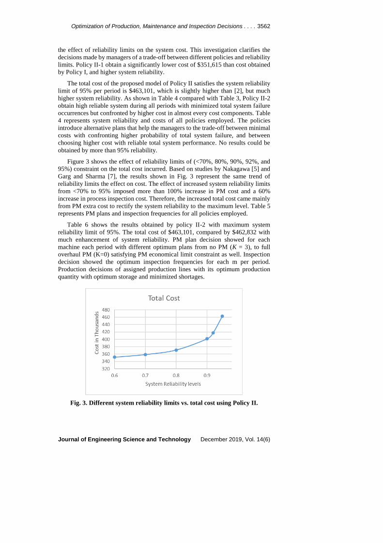
Figure 3 shows the effect of reliability limits of (<70%, 80%, 90%, 92%, and

95%) constraint on the total cost incurred. Based on studies by Nakagawa [5] and

Garg and Sharma [7], the results shown in Fig. 3 represent the same trend of

reliability limits the effect on cost. The effect of increased system reliability limits

from <70% to 95% imposed more than 100% increase in PM cost and a 60%

increase in process inspection cost. Therefore, the increased total cost came mainly

from PM extra cost to rectify the system reliability to the maximum level. Table 5

represents PM plans and inspection frequencies for all policies employed.

Table 6 shows the results obtained by policy II-2 with maximum system

reliability limit of 95%. The total cost of $463,101, compared by $462,832 with

much enhancement of system reliability. PM plan decision showed for each

machine each period with different optimum plans from no PM (K = 3), to full

overhaul PM (K=0) satisfying PM economical limit constraint as well. Inspection

decision showed the optimum inspection frequencies for each m per period.

Production decisions of assigned production lines with its optimum production

quantity with optimum storage and minimized shortages.

Fig. 3. Different system reliability limits vs. total cost using Policy II.



Table 4. Policy II 1, 2 results cost and system reliability comparison.

𝑹𝑺,𝒕 TC CP

𝑪𝑷𝑴𝑻, 𝑪𝑭𝑹𝑻

Inspection

cost

Policy

II-1 no Rs 0.80, 0.70, 0.89, 0.73 0.95, 0.85 351615 274327 43187 34100

Policy

II-2 Rs ≥ 0.9 0.96, 0.94, 0.95, 0.96, 0.94, 0.94 401398 285818 67690 47889

Policy

II-2 Rs ≥ 0.95 0.95, 0.95, 0.96, 0.95, 0.96,0.95 463101 317238 90164 55699

Table 5. PM plans and inspection frequencies for all policies employed.

Policy II-1 no Rs PMk,m,t 0,0,3,0,1,0,1,3,0,2,1,3,1,1,3,3,0,3

IIFm,t 7,7,16,7,15,7,13,17,4,9,13,17,9,11,14,18, 3,7

Policy II-2 Rs ≥ 0.9 PMk,m,t 0,1,3,1,1,2,3,1,0,3,3,3,3,0,3,0,0,0

IIFm,t 7,15,20,22,22,23,14,17,4,9,14,18,10,3,7,3,3,3

Policy II-2 Rs ≥ 0.95 PMk,m,t 1,3,1,3,1,2,2,0,1,0,2,2,0,3, 0,3,0,0

IIFm,t 20,22,23,23,23,22,13,4,9,4,9,13,3,7,3,7,3,3

Table 6. Results obtained by PM Policy II-2 with reliability limit 95%.

TC Cp CFR, CPM Inspection

cost

463101 317238 90164 55699

PM plan K t = 1 t = 2 t = 3 t = 4 t = 5 t = 6

M1 1 3 1 3 1 2

M2 2 0 1 0 2 2

M3 0 3 0 3 0 0

IIFm,t

M1 20 22 23 23 23 22

M2 13 4 9 4 9 13

M3 3 7 3 7 3 3

Qp,m,t

P1

M1 2168 1996 1948 1801 1799 1720

M2 983 998 992 998 992 984

M3 0 0 0 0 0 0

P2

M1 0 0 0 0 0 0

M2 0 0 0 0 0 0

M3 2500 2000 1500 2506 2997 2997

𝑺𝒑,𝒎,𝒕

P1

M1 1 1 1 1 1 1

M2 1 1 1 1 1 1

M3 0 0 0 0 0 0

P2

M1 0 0 0 0 0 0

M2 0 0 0 0 0 0

M3 1 1 1 1 1 1

IQp,t

P1 0 0 85 384 2175 0

P2 0 0 0 1006 503 0

BQp,t

P1 349 1355 0 0 0 121

P2 0 0 0 0 0 0



6.4. Comparison with other solution methods

The results of the proposed model are compared to the results obtained by Fakher

et al. [31] with the same data inputs to validate the optimization method of the

proposed model. The result of the total cost of the proposed model and solution

method is $321,558, while the result of Fakher et al. [31] is $331,335 using Tabu

search hybrid Genetic Algorithm solution method. This result obtained, not only

the lower total cost but also not violating PM cost constraint of not exceeding

$1500 per period. In addition, the results obtained satisfies the reliability

constraint for each period of not exceeding 98% reliability.

The results of the proposed model are compared as well to the results obtained

by Nourelfath et al. [32]. They used an exact solution algorithm for the solution

of the problem. They proposed an inspection-maintenance model with intervals

of 0.2 months and 0.3 months. Two PM plan can be implemented each inspection

time, the plan with 100% PM plan, and the plan with 50% of PM plan. They

concluded that the inspection interval of 0.3 months with 100% PM plan obtains

the lowest cost of $107,930 for the model while the same decision obtained by

the proposed model, but with a lower cost of $107,382, with the same fulfilment

of production and inventory decisions obtained by the proposed MILP method.

See Table 7.

Table 7. Results of two solution methods

compared to the proposed method.

Results Fakher et al. [2] Fakher et al. [31] Nourelfath et al. [32]

TC = $462,832 TC = $331,335 TC = $107,930

Proposed method

no. RS,t TC = $462,688 TC = $321,428 TC = $107,382

Proposed method

with RS,t

TC = $463,101

RS,t > 95%

TC = $321,558

𝑅𝑆,𝑡>98% TC = $107,382

7. Conclusions

An integrated production, maintenance, and inspection mathematical model are

proposed and several conclusions are given:

There are significant interdependencies between production, maintenance, and

inspection decisions.

The production system is composed of multiple production lines producing multi-

products assigned to production lines for delivery in lots during a specified period.

The production system is attached to PM activities, failures repairs, and

process/product inspections.

The model objective minimizes total costs subject to constraints of machines

availability and PM cost limitations with maximum reliability limit to enhance

decision maker’s confidence.

Genetic Algorithms are utilized to find the optimum PM plan and inspection

decisions for each production line each period, while a Mixed Integer Linear

Program MILP model is used to find the production decisions.

Results showed the importance of PM plan costs and maximum reliability

constraints and their effect on the overall cost of the system compared with

previous studies.



Nomenclatures

a0m,t Age of m at the start of period t or after immediate PM action,

month

a1m,t Age of m at the end of processing time period t, month

BQp,t Backorder quantity of product p from shortage at time t

Cbp Backorder penalty cost per unit of unsatisfied product p, $

Ccp Cost of product p quality checking, $

Cfrm Cost per failure repair for production line m, $

CFRT Total cost of failure repair for all periods t of T, $

Chp Holding cost per unit of product p stored, $

Cinm Production line m per inspection activity cost, $

Cpmm,t,k Cost of PM for m action activity plan k at period t, $

CPMT Total cost of preventive maintenance for all periods t of T, $

Cprp,m Production cost for product p in production line/machine m, $

CPT Production cost for all period t, of T, $

Crcm Re-set machines configuration cost for production line m, $

Csp,m Set-up cost as setting production line m configuration for product, $

Dp,t Market demand for product p in period t

FFm,t Expected failure frequencies of m within a time t, (failure/month)

Fm(y) Probability density function of time to failure for m

IIFm,t Inspection frequencies for production line m in period t,

(inspection/month)

IQp,t Inventory quantity of product p stored from overproduction /t

LQp,t Lot quantity produced of product p from assigned m at period t

MTm(km) Maintenance time required for m at PM activity plan k

m, M Production lines/machines indices

PMk,m,t Preventive Maintenance plan k for machine m at period t

PMGCt Preventive maintenance cost limit at period t, $

PRp,m Initial production rate/unit of time for product p on m, (P/month)

PTm,t Net production time available of production line m at period t

Qp,m,t Production quantity of product p assigned to production line/t

RS,t Reliability of system at period t

RTm Repair time required for machine m, month

Sp,m,t Set-up binary variable of setting product p on m at period t

t, T Time periods indices

Greek Symbols

m,m Shape Weibull distribution parameter and characteristic time

parameter for production line m for time to defect

m,m Shape and time Weibull distribution parameters for time to failure

Abbreviations

GA Genetic Algorithms

MILP Mixed Integer Linear Programming

PL Production Line

PM Preventive Maintenance



References

1. Ben-Daya, M. (1999). Integrated production maintenance and quality model

for imperfect processes. IIE Transactions, 31(6), 491-501.

2. Fakher, H.B.; Nourelfath, M.; and Gendreau, M. (2016). Joint maintenance and

production planning in a deteriorating system: model and solution method.

Proceedings of the 11th International Conference on Modeling, Optimization

and Simulation (MOSIM). Montréal, Québec, Canada, 10 pages.

3. Bajestani, M.A.; Banjevic, D.; and Beck, J.C. (2014). Integrated maintenance

planning and production scheduling with Markovian deteriorating machine

conditions. International Journal of Production Research, 52(24), 7377-7400.

4. Pham, H.; Wang, H. (1996). Imperfect maintenance. European Journal of

Operational Research, 94(3), 425-438

5. Nakagawa, T. (2005). Maintenance theory of reliability. London, United

Kingdom: Springer-Verlag.

6. Wang, H. (2002). A survey of maintenance policies of deteriorating systems.

European Journal of Operational Research, 139(3), 469-489.

7. Garg, H.; and Sharma, S.P. (2013). Reliability-redundancy allocation problem

of pharmaceutical plant. Journal of Engineering Science and Technology, 8(2),

190-198.

8. Supriatna, A.; Singgih, M.L.; Kurniati, N.; and Widodo, E. (2016). Preventive

maintenance strategies: Literature review and directions. Proceedings of the

7th International Conference on Operations and Supply Chain Management.

Phuket, Thailand, 127-139.

9. Gilardoni, G.L.; Guera de Toledo, M.L.; Freitas, M.A.; and Colosimo, E.A.

(2016). Dynamics of an optimal maintenance policy for imperfect repair

models. European Journal of Operational Research, 248(3), 1104-1112.

10. Mabrouk, A.B.; Chelbi, A.; and Radhoui, M. (2016). Optimal imperfect

maintenance strategy for leased equipment. International Journal of

Production Economics, 178, 57-64.

11. Aghezzaf, E-H.; and Najid, N.M. (2008). Integrated production planning and

preventive maintenance in deteriorating production systems. Information

Sciences, 178(17), 3382-3392.

12. Hafidi, N.; El Barkany, A.; and Mahmoudi, M. (2017). Integration of

maintenance and production strategies under subcontracting constraint:

Classification and opportunity. Journal of Mechanical Engineering and

Sciences, 11(3), 2856-2882.

13. Porteus, E.L. (1986). Optimal lot sizing, process quality improvement and

setup cost reduction. Operations Research, 34(1), 137-144.

14. Lee, H.L.; and Rosenblatt, M.J. (1987). Simultaneous determination of

production cycle and inspection schedule in a production system. Management

Sciences, 33(9), 1125-1136.

15. Groenevelt, H.; Pintelon, L.; and Seidmann, A. (1992). Production lot sizing

with machine breakdowns. Management Science, 38(1), 104-123.

16. Buzacott, J.A.; and Shanthikumar, J.G. (1993). Stochastic models of

manufacturing systems. Upper Saddle River, New Jersey, United States of

America: Prentice Hall.



17. Van der Duyn Schouten, F.A.; and Vanneste, S.G. (1995). Maintenance

optimization of a production system with buffer capacity. European Journal

of Operational Research, 82(2), 323-338.

18. Meller, R.D.; and Kim, D.S. (1996). The impact of preventive maintenance on

system cost and buffer size. European Journal of Operational Research, 95(3),

577-591.

19. Rezg, N.; Xie, X.; and Mati, Y. (2004). Joint optimization of preventive

maintenance and inventory control in a production line using simulation.

International Journal of Production Research, 42(10), 2029-2046.

20. Chelbi, A.; and Rezg, N. (2006). Analysis of a production/inventory system

with randomly failing production unit subjected to a minimum required

availability level. International Journal of Production Economics, 99(1-2),

131-143.

21. Lin, G.C.; and Gong, D.-C. (2006). On a production-inventory system of

deteriorating items subject to random machine breakdowns with a fixed repair

time. Mathematical and Computer Modelling, 43(7-8), 920-932.

22. Aghezzaf, E.F.; Jamali, M.A.; and Ait-Kadi, D. (2007). An integrated

production and preventive maintenance planning model. European Journal of

Operational Research, 181(2), 679-685.

23. El-Ferik, S. (2008). Economic production lot-sizing for an unreliable machine

under imperfect age-based maintenance policy. European Journal of

Operational Research, 186(1), 150-163.

24. Najid, N.M.; Alaoui-Selsouli, M.; and Mohafid, A. (2011). An integrated

production and maintenance planning model with time windows and shortage

cost. International Journal of Production Research, 49(8), 2265-2283.

25. Nourelfath, M.; Chatelet, E.; and Nahas, N. (2012). Joint redundancy and

imperfect preventive maintenance optimization for series-parallel multi-state

degraded systems. Reliability Engineering and System Safety, 103, 51-60.

26. Alaoui-Selsoulia, M.; Mohafid, A.; and Najid, N.M. (2012). Lagrangian

relaxation based heuristic for an integrated production and maintenance

planning problem. International Journal of Production Research, 50(13),

3630-3642.

27. Fitouhi, M.-C.; and Nourelfath, M. (2014). Integrating noncyclical preventive

maintenance scheduling and production planning for multi-state systems.

Reliability Engineering & System Safety, 121, 175-186.

28. Xiang, Y.; Cassady, C.R.; Jin, T.; and Zhang, C.W. (2014). Joint production

and maintenance planning with machine deterioration and random yield.


29. Aghezzaf, E.H.; Khatab, A.; and Le Tam, P. (2016). Optimizing production

and imperfect preventive maintenance planning’s integration in failure -

prone manufacturing systems. Reliability Engineering and System Safety,

145, 190-198.

30. Cheng, G.Q.; Zhou, B.H.; and Li, L. (2016). Joint optimisation of production

rate and preventive maintenance in machining systems. International Journal

of Production Research, 54(21), 6378-6394.



31. Fakher, H.B.; Nourelfath, M.; and Gendreau, M. (2016). A cost minimisation

model for joint production and maintenance planning under quality constraints.


32. Nourelfath, M.; Nahas, N.; and Ben-Daya, M. (2016). Integrated preventive

maintenance and production decisions for imperfect processes. Reliability

Engineering and System Safety, 148, 21-31.

33. Abdul Rahim, M.K.I.; Nadarajan, S.S.R.; and Ahmad, M.A. (2017). Solving

the single-period inventory routing problem with the deterministic approach.

Journal of Engineering Science and Technology (JESTEC), Special Issue on

ISSC’2016, 158-168.

34. Dallery, Y.; and Gershwin, S.B. (1992). Manufacturing flow line systems: A

review of models and analytical results. Queueing Systems, 12, 88 pages.

35. Gendreau, M.; and Potvin, J.-Y. (2010). Handbook of metaheuristics (2nd ed.).

New York, United States of America: Springer Science + Business Media.

Appendix A

Sample Calculations of Numerical Experiment and Solution Steps

Building GA’s solution chromosome of PM plans ranges from K =

{0,1,2,3} with a cost of each plan Cpm (K) as given in Table 2 for each

production line m, and period t. M = 3 PLs , T =6 periods, then

chromosome size = 18.

Calculate new age a01,1 for PL1 at period 1 using Eq. (11), knowing age

a11,0 = 3 of previous period. Assuming PM plan obtained from step 1 is k

= 1, for PL 1 at period 1 with its cost Cpm1,1,1 = $500. The maximum PM

plan cost Cpm1(Max) = $ 3000. Then a11,1 = 2.6.

Repeat step 2 for each PL and each period.

Check the PM cost constraint Eq. (17) for each period for not exceeding

PMGCt = $500 each period. If constraint Eq. (17) is not fulfilled at any of

the periods, the whole solution is excluded and return back to step 1 for a

new one. If Eq. (17) is fulfilled, go to next step.

o i.e., for a set of K{1,2,0} summation of, Cpm1,1,1 = $500, Cpm2,1,2 =

$200, Cpm3,1,0 = $4000 must be less or equal PMGCt = $5000.

Calculate the system reliability RS,t Eq. (13) for each period then check the

reliability constraint Eq. (14) of not exceeding Rlimit. If constraint Eq. (14)

is not fulfilled at any of the periods, the whole solution is excluded and

return to step 1 for a new one. If Eq. (14) is fulfilled, go to next step.

Evaluate maintenance CPMT and failure repair cost CFRT using Eqs. (10),

(15), and (16).

Evaluate inspection frequencies decision IIFm,t and costs using Eqs. (20) to (22).

Calculate the available time for production for each PL. using Eq. (7).

Evaluate the production decisions MILP problem using CPLEX solver.

Using Eqs. (1), (3), and (4) and satisfying production constraints Eqs. (2),

(5), and (6).

Obtain the decision variables and objective function.

OPTIMIZATION OF PRODUCTION, MAINTENANCE …jestec.taylors.edu.my/Vol 14 issue 6 December...

Documents

Transcript of OPTIMIZATION OF PRODUCTION, MAINTENANCE …jestec.taylors.edu.my/Vol 14 issue 6 December...