OPTIMIZATION OF POCKET MILLING TOOL PATH FOR CHATTER ...
106
OPTIMIZATION OF POCKET MILLING TOOL PATH FOR CHATTER AVOIDANCE AND REDUCED MACHINING TIME LUCY WANJA KARIUKI MASTER OF SCIENCE (Mechatronic Engineering) JOMO KENYATTA UNIVERSITY OF AGRICULTURE AND TECHNOLOGY 2017
Transcript of OPTIMIZATION OF POCKET MILLING TOOL PATH FOR CHATTER ...

OPTIMIZATION OF POCKET MILLING TOOL PATH
FOR CHATTER AVOIDANCE AND REDUCED
MACHINING TIME
LUCY WANJA KARIUKI
MASTER OF SCIENCE
(Mechatronic Engineering)
JOMO KENYATTA UNIVERSITY OF
AGRICULTURE AND TECHNOLOGY
2017

Optimization of pocket milling tool path for chatter avoidance and
reduced machining time
Lucy Wanja Kariuki
A thesis submitted in partial fulfillment for the degree of Master of
Science in Mechatronic Engineering in the Jomo Kenyatta University
of
Agriculture and Technology
2017

DECLARATION
This thesis is my original work and has not been presented for a degree in any
other University.
Signature:....................................... Date..................................
Lucy Wanja Kariuki
This thesis has been submitted for examination with our approval as the Univer-sity
Supervisors.
Signature:....................................... Date..................................
Prof. Eng. Benard W. Ikua, (PhD)
JKUAT, Kenya
Signature:....................................... Date..................................
Prof. George N. Nyakoe, (PhD)
JKUAT, Kenya
i

DEDICATION
I dedicate this work to my parents, my husband Henry, and my sons Jayden and
Manuel. Thank you for always believing in me.
ii

ACKNOWLEDGEMENT
First and foremost, my gratitude goes to the Almighty God for enabling me to
pursue this endevour. Secondly, I would like to acknowledge my supervisors, Prof.
Eng. B. W. Ikua and Prof. G. N. Nyakoe for their invaluable guidance and advice
throughout my studies.
I also wish to thank Jomo Kenyatta University of Agriculture and Technology
for funding my studies. My appreciation also goes to the staff of Departments
of Mechatronic Engineering and Mechanical Engineering for all their facilitation
and assistance.
I acknowledge the administration and staff of National Youth Service(NYS) En-
gineering Institute for allowing me to use their machines and equipment to carry
out my experiments.
Finally I wish to acknowledge my coursemates Brenda W. Nyota and Martin
R. Maina, and all postgraduate students who walked this journey with me and
offered invaluable input and criticism.
God bless you all.
iii

TABLE OF CONTENTS
DECLARATION . . . . . . . . . . . . . . . . . . . . . . . . . . . . . . i
DEDICATION . . . . . . . . . . . . . . . . . . . . . . . . . . . . . . . ii
ACKNOWLEDGEMENTS . . . . . . . . . . . . . . . . . . . . . . . . iii
TABLE OF CONTENTS . . . . . . . . . . . . . . . . . . . . . . . . . iv
LIST OF FIGURES . . . . . . . . . . . . . . . . . . . . . . . . . . . . vii
LIST OF TABLES . . . . . . . . . . . . . . . . . . . . . . . . . . . . . ix
LIST OF APPENDICES . . . . . . . . . . . . . . . . . . . . . . . . . . x
NOMENCLATURE . . . . . . . . . . . . . . . . . . . . . . . . . . . . xi
ABSTRACT . . . . . . . . . . . . . . . . . . . . . . . . . . . . . . . . xii
CHAPTER 1 INTRODUCTION 1
1.1 Background . . . . . . . . . . . . . . . . . . . . . . . . . . . . . . 1
1.2 Tool paths . . . . . . . . . . . . . . . . . . . . . . . . . . . . . . . 3
1.3 Problem Statement . . . . . . . . . . . . . . . . . . . . . . . . . . 6
1.4 Objectives . . . . . . . . . . . . . . . . . . . . . . . . . . . . . . . 7
1.5 Significance of study . . . . . . . . . . . . . . . . . . . . . . . . . 8
CHAPTER 2 LITERATURE REVIEW 9
2.1 Geometry of flat end mill . . . . . . . . . . . . . . . . . . . . . . . 9
2.2 Milling operations . . . . . . . . . . . . . . . . . . . . . . . . . . . 10
2.2.1 Up milling . . . . . . . . . . . . . . . . . . . . . . . . . . . 11
2.2.2 Down milling . . . . . . . . . . . . . . . . . . . . . . . . . 11
2.3 Modelling of end milling forces . . . . . . . . . . . . . . . . . . . . 12
2.4 Identification of Cutting Constants . . . . . . . . . . . . . . . . . 16
2.4.1 Determination of cutting constants from orthogonal cutting 16
2.4.2 Orthogonal to oblique cutting transformation . . . . . . . 18
2.4.3 Mechanistic approach . . . . . . . . . . . . . . . . . . . . . 19
iv

2.5 Calculation of instantaneous depth of cut . . . . . . . . . . . . . . 21
2.6 Model system dynamics . . . . . . . . . . . . . . . . . . . . . . . 22
2.6.1 Dynamic regenerative undeformed chip thickness . . . . . 23
2.7 Vibrations in milling . . . . . . . . . . . . . . . . . . . . . . . . . 25
2.8 Fundamentals of free and forced vibrations . . . . . . . . . . . . . 25
2.9 Chatter Stability Criterion . . . . . . . . . . . . . . . . . . . . . . 27
2.9.1 Time Domain Simulation . . . . . . . . . . . . . . . . . . . 28
2.9.2 Frequency Domain Simulation . . . . . . . . . . . . . . . . 29
2.9.3 Stability lobes theory . . . . . . . . . . . . . . . . . . . . . 30
2.10 Tool path optimization . . . . . . . . . . . . . . . . . . . . . . . . 31
CHAPTER 3 METHODOLOGY 37
3.1 Identification of cutting constants . . . . . . . . . . . . . . . . . . 37
3.2 Modelling of cutting force . . . . . . . . . . . . . . . . . . . . . . 38
3.2.1 Cutter engagement boundaries . . . . . . . . . . . . . . . . 41
3.3 Dynamic milling system model . . . . . . . . . . . . . . . . . . . . 43
3.4 Experimental work . . . . . . . . . . . . . . . . . . . . . . . . . . 46
3.4.1 Tool path generation and simulation . . . . . . . . . . . . 47
3.4.2 Fixture and workpiece design and preparation . . . . . . . 49
3.4.3 Dynamometer calibration . . . . . . . . . . . . . . . . . . 49
3.4.4 Verification of cutting force models . . . . . . . . . . . . . 50
3.5 Chatter stability criterion . . . . . . . . . . . . . . . . . . . . . . 51
3.6 Optimization of pocket milling parameters . . . . . . . . . . . . . 54
CHAPTER 4 RESULTS AND DISCUSSION 56
4.1 Determination of cutting constants . . . . . . . . . . . . . . . . . 56
4.2 Verification of static and dynamic cutting force models . . . . . . 57
4.3 Effect of depth of cut on cutting force . . . . . . . . . . . . . . . . 59
4.4 Effect of feedrate on cutting force . . . . . . . . . . . . . . . . . . 60
v

4.5 Cutting force waveforms for different tool path strategies . . . . . 61
4.6 Effect of tool path strategy on cycle time . . . . . . . . . . . . . . 64
4.7 Determination of chatter boundary . . . . . . . . . . . . . . . . . 65
4.8 Effect of tool path strategy on chatter vibration . . . . . . . . . . 66
4.9 Variation of vibration with feedrate . . . . . . . . . . . . . . . . . 68
CHAPTER 5 CONCLUSION AND RECOMMENDATIONS 72
5.1 Conclusion . . . . . . . . . . . . . . . . . . . . . . . . . . . . . . . 72
5.2 Recommendations . . . . . . . . . . . . . . . . . . . . . . . . . . . 73
REFERENCES 74
APPENDICES 78
vi

LIST OF FIGURES
Figure 1.1 C ontour-parallel tool path . . . . . . . . . . . . . . . . . . 4
Figure 1.2 D irection-parallel tool path . . . . . . . . . . . . . . . . . . 5
Figure 2.1 End mill cutter . . . . . . . . . . . . . . . . . . . . . . . . 9
Figure 2.2 Model of helical end mill . . . . . . . . . . . . . . . . . . . 10
Figure 2.3 Up milling Down milling . . . . . . . . . . . . . . . 12
Figure 2.4 Cutter model . . . . . . . . . . . . . . . . . . . . . . . . . 13
Figure 2.5 Force components on cutter . . . . . . . . . . . . . . . . . 13
Figure 2.6 Geometry of chip . . . . . . . . . . . . . . . . . . . . . . . 21
Figure 2.7 Chip formation in milling . . . . . . . . . . . . . . . . . . 22
Figure 2.8 Mass, spring and damping model of a single degree of free-
dom system . . . . . . . . . . . . . . . . . . . . . . . . . . . . . . 26
Figure 2.9 Free vibration . . . . . . . . . . . . . . . . . . . . . . . . . 27
Figure 2.10 Illustration of time and frequency domains . . . . . . . . . 29
31Figure 2.11 Stability LobeDiagram . . . . . . . . . . . . . . . . . . . .
Figure 2.12 Screenshot of tool path strategies available for machining a
rectangular pocket using Mastercam R© . . . . . . . . . . . . . . . . 32
Figure 3.1 Experimental setup for determination of baseline data. . . 37
Figure 3.2 Cutter modelling . . . . . . . . . . . . . . . . . . . . . . . 38
Figure 3.3 Flowchart of milling force simulation . . . . . . . . . . . . 40
Figure 3.4 Start and exit angles . . . . . . . . . . . . . . . . . . . . . 41
Figure 3.5 Variation of cutting force with cutter rotation angle . . . . 42
Figure 3.6 Model for dynamic regenerative chip thickness . . . . . . . 44
Figure 3.7 (a) Parallel spiral tool path (b) Zigzag tool path (c) True
spiral tool path . . . . . . . . . . . . . . . . . . . . . . . . . . . . 47
vii

Figure 3.8 Machining times when using dierent tool path strategies
(Rectangular pocket, 30 mm by 20 mm by 10 mm) . . . . . . . . 48
Figure 3.9 Experimental setup for dynamometer calibration . . . . . . 49
Figure 3.10 Experimental setup . . . . . . . . . . . . . . . . . . . . . . 50
Figure 3.11 Photograph of the experimental setup . . . . . . . . . . . . 52
Figure 3.12 Frequency spectrum (f=0.08, a=0.5 mm, N=450 rpm) . . 53
55Figure 3.13 Optimization flowchart . . . . . . . . . . . . . . . . . . . .
Figure 4.1 Force waveforms for side milling (f=0.2 mm/t, N=705
min−1,a= 5mm,nt=1) . . . . . . . . . . . . . . . . . . . . . . . . . 56
Figure 4.2 Waveforms for predicted and measured cutting forces . . . 58
Figure 4.3 Variation of cutting force with depth of cut . . . . . . . . . 60
Figure 4.4 Variation of cutting force with feedrate . . . . . . . . . . . 61
Figure 4.5 Cutting force waveforms for various tool path strategies . . 63
Figure 4.6 Cycle times for dierent tool path strategies . . . . . . . . 64
Figure 4.7 Plot of chatter values . . . . . . . . . . . . . . . . . . . . . 66
Figure 4.8 Effect of tool path strategy on chatter occurrence . . . . . 69
Figure 4.9 Effect of tool path strategy on chatter vibration . . . . . . 70
Figure 4.10 Frequency analysis of vibration at different feedrates . . . 71
viii

LIST OF TABLES
Table 3.1 Model inputs . . . . . . . . . . . . . . . . . . . . . . . . . . . 39
Table 4.1 Average cutting forces per tooth period . . . . . . . . . . . . . 56
Table 4.2 Cutting and edge coefficients . . . . . . . . . . . . . . . . . . . 56
Table 4.3 Standard milling parameters . . . . . . . . . . . . . . . . . . . 56
Table 4.4 Table of comparison for measured and predicted forces . . . . . 58
Table 4.5 Variation of cutting force with depth of cut . . . . . . . . . . . 58
Table 4.6 Variation of cutting force with feedrate . . . . . . . . . . . . . 59
Table 4.7 Table of force ratios . . . . . . . . . . . . . . . . . . . . . . . 64
ix

LIST OF APPENDICES
Appendix A: Instrument calibration . . . . . . . . . . . . . . . . . . 79
Appendix B: Matlab simulation of milling force . . . . . . . . . . . . 82
Appendix C: Flowchart of simulation . . . . . . . . . . . . . . . . . . 85
Appendix D: Solution of Dynamic equations . . . . . . . . . . . . . . 86
Appendix E: Labview front panels . . . . . . . . . . . . . . . . . . . . 89
Appendix F: Experimental setup . . . . . . . . . . . . . . . . . . . . 91
Appendix G: Publications . . . . . . . . . . . . . . . . . . . . . . . . 93
x

NOMENCLATURE
a axial depth of cut
Ac chip area
b nominal depth of cut
c damping coefficient
D cutter diameter
f feedrate
Fd dynamic cutting force, N
Ff friction force, N
Fn normal force against friction, N
Fs static cutting force, N
Fx cutting force in x direction, N
Fy cutting force in y direction, N
Fz cutting force in z direction, N
h undeformed chip thickness
hc chip thickness
hd instantaneous dynamic chip thickness
hs static chip thickness, mm
k stiffness constant
Kac axial cutting coefficient
Krc radial cutting/feed force coefficient
Ktc tangential cutting coefficient
Kae axial edge coefficient
Kre radial edge coefficient
Kte tangential edge coefficient
m mass, g
N spindle speed, cycles per minute
xi

nt number of teeth
rc chip thickness ratio
αr tool rake angle,
β friction angle
γ helix angle,
µ coefficient of friction
φ rotational angle
φex rotational angle at end of engagement
φst rotational angle at start of engagement
φp pitch angle,
φc shear angle,
lag angle
ρ ratio of dynamic to static cutting force
τs shear stress, N/mm2
xii
ABSTRACT
Modern Computer Numerical Control (CNC) machines and Computer Aided
Manufacturing (CAM) systems have become quite sophisticated and can ma-
chine geometrically feasible pocket profiles. M ore t han 8 0% o f a ll mechanical
parts which are manufactured by milling machines can be cut by Numerical Con-
trol (NC) pocket machining, which involves the removal of material within a
closed boundary. Pocket milling is applied in the manufacture of dies and molds,
and in the manufacture of aerospace and aircraft parts.
Most of the current Computer Aided Design and Computer Aided Manufacturing
(CAD/CAM) systems used in CNC machines, such as Computer Aided Three-
dimensional Interactive Application (CATIA) and Mastercam, provide the ca-
pability of generating NC pocket milling instructions based on the geometric
definition o f a w ork p iece a nd t he c utter, t hus a utomating p art programming.
However, the generation or selection of tool path is, in most cases, based on oper-
ator’s experience and intuition. There is no consideration of the dynamic effects
of the cutting process. This presents shortcomings that limit the productivity of
a CNC machining system since the efficiency of the tool path strategy impacts
on the overall efficiency of the machining process.
In this work, mathematical models for predicting static and dynamic cutting
forces in pocket milling were developed in MATLAB R© and verified experimentally.
In the dynamic cutting force model, the instantaneous undeformed chip thickness
was modelled to include the dynamic modulations caused by the tool vibrations so
that the dynamic regeneration effect which leads to chatter is taken into account.
This model was found to be more accurate in predicting cutting forces than the
commonly used static models.
A chatter stability prediction criterion was proposed in which a force ratio defined
xiii

as the ratio of maximum dynamic cutting force to maximum static cutting force
was employed as an indicator of chatter occurrence. This ratio has a limit value
beyond which the machining process becomes unstable and is dependent on the
cutter and workpiece materials. A weighting criteria was applied so as to optimize
the tool path generated for chatter avoidance, minimizing forces acting on the
tool and minimizing machining time.
Experiments were carried out using an 8mm HSS helical cutter and Aluminium
7075-0 workpiece and the limiting value of force ratio was 1.238. The experimental
results were in good agreement with the prediction model.
The influence of roughing tool path strategy on machining time, cutting force
and chatter vibration was investigated and analysed, for zigzag, parallel spiral and
true spiral tool paths. The zigzag tool path was found to have the least machining
time, while the true spiral tool path was found to have the least average cutting
forces.
The thesis presents an investigation and analysis of end milling of pockets and the
influence of roughing tool path strategy on the resultant cutting forces, chatter
vibrations and machining time.
xiv

CHAPTER 1
INTRODUCTION
1.1 Background
Metal machining is the most dominant and most important operation in the
manufacturing industry [1]. Among all the different metal machining processes,
milling is one of the most widely used due to its flexibility i n p r oducing a wide
range of products. With the competitiveness of manufacturing industries today,
it is a continuing challenge to produce products of the highest possible quality,
with the least amount of time and at a low cost. In the machining industry,
cost-effectiveness and product quality can be achieved through optimization of
the machining processes [2].
Modern CNC machines have become quite sophisticated but an efficient tool path
is very crucial. The generation or selection of tool path based on the geometric
definition of a work piece and the cutter without consideration of dynamic factors
limits the productivity of a CNC machining system.
One of the most common operations in machining metal parts is pocket milling.
This involves the manufacture of a part from a billet or forging by removing all
material inside a closed boundary to a fixed d e pth. I t i s a lso r eferred t o a s 2.5D
machining since all the machining is initially done in one plane, with a single
dimension in the third axis at each point (2D). The depth in the third axis is
however increased gradually, eventually achieving machining in three dimensions.
These pockets may have straight edges, curved edges or a combination of both.
The cutting tools used in this operation are flat-end m i lls w i th t w o o r more
flutes. M ostly, t hey a re made o f h igh s peed s teel(HSS), c arbide, while s ome have
Titanium coatings.
1
More than 80% of all mechanical parts which are manufactured by milling ma-
chines can be cut by Numerical Control (NC) pocket machining [3]. This is based
on the fact that most mechanical parts consist of faces parallel or normal to a
single plane. Also, free-form objects can be produced from a block workpiece
by 2.5D roughing (pocketing) and 3D-5D finishing. The efficiency of a pocket
milling tool path is therefore quite important in Computer Aided Manufacturing
(CAM), and thus, improvement of tool paths can have a widespread impact in
the manufacturing industry.
Most of the current Computer Aided Design and Computer Aided Manufactur-
ing (CAD/CAM) systems, such as Computer Aided Three-dimensional Inter-
active Application (CATIA), Computer Augmented Design and Manufacturing
(CADAM) and Mastercam R©, provide the capability of generating NC machining
instructions based on the geometric definition of a work piece and the cutter,
thus automating part programming. However, other process parameters such as
values of the spindle speed, feed rate, depth-of-cut and the cutting direction have
to be decided and specified by the part programmer. Since most decisions on
CNC machining parameters are made based on the intuition and experience of
the operator, these processes are often carried out at conditions that are not opti-
mal. This results in products of compromised surface quality, while using longer
than necessary machining times, and hence shortening tool life.
Extensive research towards optimization of machining parameters such as spindle
speed, feedrate and depth of cut has been carried out in the recent past. However,
optimization of tool path has not received as much attention.
2

1.2 Tool paths
Tool path refers to a series of coordinate locations that a cutting tool follows in
the machining process. Traditionally, tool paths are classified into two categories,
roughing and finishing tool p a ths. A roughing tool path is used in the CAD/CAM
CNC programming phase for removing most of the material, as accurately and
as efficiently as possible. Some types of roughing tool paths are:
• Face milling tool paths
• Profile milling tool paths
• Pocket milling tool paths
• Engraving tool paths
• Thread milling tool paths
Finishing tool paths are then used to remove a small amount of material and to
give the part the desired surface quality in the least amount of time to complete
the machining process. Tool path generation softwares have been under devel-
opment giving rise to more more efficient, faster and more robust tool paths, in
terms of what can be achieved during machining.
A wide choice of roughing tool path strategies is provided in CAD/CAM software.
For example, Mastercam R© provides up to seven tool path strategies for a simple
rectangular-pocket milling operation. This leaves wide room for improvement
of tool path efficiency. Efficiency of tool paths has been improved by creating
longer path sections which maintains cutting force near constant, rounding corner
sections and ensuring few and gradual changes in cutting direction.
Tool path approaches available in CAD/CAM systems for milling of pockets can
be broadly classified into two categories, contour-parallel and direction parallel
3

tool paths. Direction-parallel approach has two major variations, unidirectional
zig and bi-directional zigzag tool paths [3].
Contour-parallel tool paths
Contour parallel tool path pattern is generated by successive offset curves along
the work boundary. The algorithms to generate this pattern use a Voronoi di-
agram or a pixel-based approach to compute the offset curves, which are linked
together to form a connected tool path. The cutter is kept in contact with
the work most of the time thus less idle time spent in retracting, positioning and
plunging [4]. It is widely used for large scale material removal. A contour-parallel
tool path is shown in Figure 1.1.
Figure 1.1. Contour-parallel tool path
Direction-parallel tool-paths: A direction-parallel tool path is illustrated in
Figure 1.2.
Zig: uni-directional In these tool paths the tool is retracted at the end of
each cut in one direction, and is retraced to the start of the new pass without
cutting on the return stroke. Tool retraction leads to a considerable amount of
idle time, during retracting the tool and returning it to the start position. It
also lengthens the machining path and could negatively affect the tool life [4].
However a consistent chip removal can be maintained.
4

Direction-parallel tool-paths:
Zigzag: bi-directional The tool cuts both in the forward and the backward
motion. The tool is not retracted at the end. As a result of minimal tool retrac-
tions, burr formation is avoided which occurs at the point of the tool leaving the
workpiece while engaged.
Figure 1.2. Direction-parallel tool path
Besides modification of tool paths generated by CAD/CAM softwares, improve-
ment of tool paths can also be done through evaluation of the quality and ef-
ficiency of the alternative solutions, in terms of factors such as cutting forces,
chatter vibrations and machining time. To achieve this, a geometric analysis of
the cutting tool as well as dynamic characteristics of the machine/tool interaction
is necessary.
Chatter, a self-excited vibration, is also a limitation of productivity with negative
effects including poor surface quality, dimensional inaccuracy, and disproportion-
ate tool wear [5]. In pocket milling, the tool paths are characterized by many
changes in direction and velocity of the tool as the tool encounters corners. Cut-
ting forces vary during tool plunging and retraction which sometimes leads to
chatter. Hence the need to study and predict its occurrence.
5

Predicting chatter occurrence is still the subject of much research but the regen-
eration theory suggested by Tobias [6] is still the most comprehensive explanation
for the occurrence of chatter vibration. A wavy surface left by a previous tooth
during milling and removed by the successive tooth may result in the chip thick-
ness growing, which in turn results in increasing vibrations. The forces on the
tool in that case increase and may chip the tool and produce a poor finish. [3].
The dynamic cutting force acting on the cutter and workpiece also significantly
determines the occurrence of self-excited chatter vibration during cutting process.
This thesis presents a model to select optimal tool path parameters for milling
pockets at minimum cycle times and cutting forces, while avoiding chatter vibra-
tion.
1.3 Problem Statement
Conventional tool-path generation strategies are designed to generate tool paths
that satisfy geometric requirements. They, however, do not put other physical
and dynamic factors into consideration; consequently, chatter and reduced tool
life are common issues in CNC machining operations, especially when machining
at high speeds and when machining hard materials such as high carbon steels
and carbides. Decisions on machining parameters are left to the intuition and
experience of the machine operator and hence . In addition, the conventional tool
paths exhibit, momentarily, rises in cutting resistance at corner sections, leading
to chatter or even tool breakage.
With the continuing challenge to produce high quality products at the lowest
cost, application of optimized tool paths is usually a missing link. There is a
need to develop algorithms that can generate a tool path that is optimal for the
6

particular pocket profile that i s being machined.
Most of the research in optimizing pocket milling tool path is specified to only one
or two tool path strategies [7–9]. By investigating the existing tool path strategies
an optimized tool path can be generated for a particular pocket profile. Chatter
vibration will be minimized by providing a smooth variation in cutting resistance
for sections where there is a sudden rise or decrease of cutting forces. This will
result in better surface quality and it will improve tool life and machining time.
This research therefore aims to optimize the pocket milling tool path with the
aim of eliminating chatter and reducing machining time.
1.4 Objectives
The main objective in this project was to develop an algorithm for determination
of optimal pocket milling process parameters, which minimize machining time,
minimize cutting forces acting on the tool and enable chatter avoidance. To
achieve this, the following specific objectives were undertaken:
1. Development of static and dynamic force models for end milling
2. Prediction of occurrence of chatter vibration for various tool path strategies
3. Development of a control algorithm to generate the optimal pocket milling
process parameters
4. Experimental evaluation of effectiveness of the proposed control algorithm
in machining of pockets
7
1.5 Significance of study
Global trends in manufacturing process are towards better quality components
and lowering cost of production. No matter how advanced a CNC machining cen-
ter is, the tool and the tool path can limit its productivity, especially considering
that conventionally, generation of tool paths is done based on the experience of
the operator. The results of this study will assist in improving the surface quality
of components made by pocket milling, and also reduce the rate of tool wear
by avoiding tool paths that exhibit work-tool chatter vibrations. Optimization of
tool path with consideration of physical and dynamic factors will improve produc-
tivity, since tool path has been described as a weak link in machining [10]. This
study will also add to the further development of tool path generation algorithms
currently in use.
8

CHAPTER 2
LITERATURE REVIEW
2.1 Geometry of flat end mill
End mills come in a variety of material, sizes and geometries. The most commonly
used are flat e nd m ills a nd b all e nd m ills. F lat e nd m ills a re o ften u sed for
roughing while ball end mills are used for finishing a nd m achining o f complex
surfaces. The teeth maybe straight (parallel to the axis of rotation) or at a helix
angle. The helix angle helps a slow engagement of the tool, thus distributing the
forces. The cutter may be right-hand (to turn clockwise) or left-hand (to turn
counterclockwise). Figure 2.1 shows a typical end milling cutter.
Figure 2.1. End mill cutter
9

2.2 Milling operations
Milling is an intermittent multi-point operation which involves feeding the work-
piece into a rotating cutter. The milling operation can generally be divided into
two categories: peripheral and face milling. In peripheral milling, the cut surface
is parallel to the axis of the cutting tool while in face milling, the working surface
is perpendicular to the axis of the cutting tool.
Helical end mills are used in peripheral milling where the walls of the part are
the target finished s urface. The helix produces a g radually i ncreasing chip load
along the flutes. Figure 2.2 shows a model of a helical end mill whereby.
Figure 2.2. Model of helical end mill
If the helix angle on the cutter is β, a point on the axis of the cutting flute lags
behind with a lag angle ψ at the depth of cut, z, which is given by
tan β =Dψ
2z(2.1)
and
=2z tan β
D(2.2)
Therefore, when the bottom end of a particular flute is at immersion angle φ,
10

a point that is axially z mm above will have an immersion angle given by (φ −
ψ). The chip thickness removed is thus different at each point. End milling
or peripheral milling comprises of two operations namely Up milling and Down
milling, which are shown in Figure 2.3 [11].
2.2.1 Up milling
In up milling, also referred to as Conventional milling, the rotation of the cutter
is against the workpiece feed direction. The entry angle is zero and the exit angle
is nonzero, thus the chip is very thin at the beginning and increases in thickness
along its length.
The cutter tends to push the work along and lift it upwards from the table,
tending to loosen the workpiece from the fixture. In up milling, chips can be
carried into the newly machined surface, causing the surface finish to be poorer
than in down milling [11].
2.2.2 Down milling
In down milling, sometimes referred to as climb milling, the direction of the cutter
rotation is the same as the feed direction. It is advantageous in that the work
piece is pulled towards the cutter eliminating loosening of the work from the
fixture or table. However, the maximum chip thickness is at the point of tooth
contact with the work piece, since the entry angle is non-zero. This results in
faster wearing of the cutter teeth especially if the work material is hard. This
method is probably the most common option on the shop floor and will normally
produce a better surface finish [11].
11

(a) (b)
Figure 2.3. (a) Up milling (b) Down milling
2.3 Modelling of end milling forces
Prediction of cutting forces is essential for design of machine tool structure and
cutting tools as well as for the planning, control and optimization of machining
processes [12]. A reliable cutting force model for the accurate prediction of cutting
forces is critical to carrying out optimal machining process planning as well as
well as for online adaptive control for efficient and precision machining.
Modelling of cutting forces is also one of the most important constraints in tool
path optimization algorithms. These force prediction models are important as
they minimize the need for experiments, thus minimizing machining cost and
time.
Modelling of cutting forces requires the knowledge of the tool geometry, part ge-
ometry as well as the cutting conditions. Tool- workpiece behaviour and perfor-
mance attributes such as tool wear, machine-tool chatter, dimensional accuracy,
surface quality and the productivity of the system can be studied based on force
analysis [13].
Several predictive cutting force models for flat-end and ball-end milling processes
have been developed [13–16]. These force models generalize the relationship be-
tween instantaneous cutting forces and the chip load distribution. Therefore they
can be applied in prediction of cutting forces for the geometries at hand.
12

In the static force model, each tooth of a helical end milling cutter is discretised
into a number of elements along the cutter axis as shown in Figure 2.4.
Figure 2.4. Cutter model
The principal forces acting on a differential element of height dz on the cutting
edge j are Tangential(dFt,j), Radial(dFr,j) and Axial(dFa,j) forces. These are
shown in Figure 2.5. Axial force is parallel to the tool axis.
Figure 2.5. Force components on cutter
Tangential (dFt,j), Radial (dFr,j) and Axial (dFa,j) forces acting on a differential
element on tooth j of height dz in the axial direction are expressed as
13

dFt,j(φ, z) = [Kt,chj(φj(z)) +Kte]dz,
dFr,j(φ, z) = [Kr,chj(φj(z)) +Kre]dz, (2.3)
dFa,j(φ, z) = [Ka,chj(φj(z)) +Kae]dz,
where the static chip thickness for the lth element at rotation angle φ is given by
hj(φ, z) = c sinφj(z). (2.4)
Here, c denotes feed per tooth.
The total cutting force is calculated by adding the effort on each edge discrete
cutting element. Cutting force is calculated based on the undeformed chip thick-
ness, cutting conditions and specific cutting coefficients [16]. The coefficients Kt,
Kr and Ka are cutting constants in tangential, radial and axial directions for the
specific cutter-workpiece combination.
These differential elemental forces are then resolved into the feed(x), normal and
axial directions using the following transformation
dFx,j(φj(z)) = −dFt,j cosφj(z)− dFr,j sinφj(z)
dFy,j(φj(z)) = dFt,j sinφj(z)− dFr,j cosφj(z) (2.5)
dFz,j(φj(z)) = dFa,j
To relate the cutting forces to the tool path geometry, the calculation of axial tool
engagement and radial depth of cut has to be done for any position. However, in
14

pocket milling the axial engagement is constant for every machining pass but the
radial depth of cut varies along the tool path. Depth of cut also influences the
occurrence of chatter vibrations, which consequently leads to faster tool wear and
poor surface quality. Predicted cutting forces are useful in avoiding tool vibration
and breakage, and reducing dimensional errors caused by tool deflections.
Literature describes various studies in modelling of cutting forces, both for flat
end milling and ball end milling. A study by Dang et al [14] proposed a cutting
force model for flat end milling. The novel feature of their model was that the
overall cutting forces caused by both the flank edge and the bottom edge cuttings
were simultaneously taken into consideration. The model showed that for small
axial depths of cut the bottom edge had a significant effect on total cutting forces.
A closed form expression for the dynamic forces in milling process, as functions
of cutting parameters and tool/workpiece geometry was presented by Wang et
al [15].
The cutting force function was characterized by the chip thickness variation and
radial cutting configuration. The analysis of cutting forces was extended into the
Fourier domain by taking the frequency multiplication of the transforms of the
three component functions.
Kline and DeVor [17] developed a flat end milling force model based on chip load
cutting geometry and the relation between cutting forces and and chip load in
thin disk-shaped sections along the cutter axis. The cutter action on each cutting
edge element in flat end milling is the same for all axial positions on the cutter.
Omar et al [16] introduced a generic and improved cutting force model. The
model simultaneously predicted the conventional cutting forces and the surface
topography during side milling operation. Effects of tool run-out, tool deflection,
system dynamics, flank face wear, and tool deflection on the surface roughness
15

were incorporated in the model. In their work, an improved technique to calculate
the instantaneous chip thickness was also presented.
2.4 Identification of Cutting Constants
2.4.1 Determination of cutting constants from orthogonal
cutting
In orthogonal cutting, the cutting edge is perpendicular to the direction of tool-
workpiece motion. The cutting forces are thus exerted in only two directions, the
tangential and the feed direction.
Cutting coefficients are determined based on three parameters, shear angle, φs,
friction angle, βa, and shear strength, τs. These parameters depend both on the
material and process. The shear angle, which is a function of rake angle, αr and
chip compression ratio, rc, is determined by
tanφc =rc cosαr
1− rc sinαr
, (2.6)
where rc is given by
rc =h
hc
where h is undeformed chip thickness and hc is chip thickness.
The orthogonal cutting tests are perfomed under different feedrates and cutting
speeds and the resultant cutting force, F, is measured. According to [18], the
tangential and feed forces can then be determined from resultant force using the
relations
16

Ft = F cos(βa − αr),
Ff = F sin(βa − αr),
where βa is the friction angle, αr is the tool rake angle and φc is the shear angle.
In terms of shear stress the forces can be expressed as
Ft = bhτs
[cos(βa − αr)
sinφc cos(φc + βa−r)
](2.7)
and
Ff = bhτs
[sin(βa − αr)
sinφc cos(φc + βa − αr)
]. (2.8)
In metal machining, the parameter specific cutting pressure or tangential cutting
force coefficient, Kt is defined as
Kt = τscos(βa − αr)
sinφccos(φc + βa − αr)(2.9)
and the feed force constant, Kr is
Kr = τssin(βa − αr)
sinφccos(φc + βa − αr)(2.10)
Attempts at theoretical evaluation of shear angle has led to two main approaches,
namely the maximum shear stress principle and the minimum energy principle
[18].
17

In the first approach, Krystof proposed a shear angle relation based on the max-
imum shear stress principle which states that shear occurs in the direction of
the maximum shear stress. The resultant force makes an angle, (φc + βa − αr),
with the shear plane and the angle between the maximum shear stress and the
principal stress must be π/4, thus leading to the shear angle relation which is
expressed as
φc =π
4− (βa − αr). (2.11)
The second approach by Merchant proposed applying the minimum energy prin-
ciple. By taking the partial derivative of the cutting power given by Pt = FtV
where V is cutting velocity and
Ft = bh
[τs
cos(βa − αr)
sinφc cos(φc + βa − αr)
]. (2.12)
The shear angle is obtained as
φc =π
4− βa − αr
2. (2.13)
2.4.2 Orthogonal to oblique cutting transformation
In the case of helical end milling, the cutting edge is not perpendicular to the feed
direction but is inclined at an angle equal to the helix angle. The tangential (Ktc),
radial (Krc) and axial (Kac) cutting coefficients for oblique cutting as proposed
by Budal et al [19] are given by
18

Ktc =τ
sinφn
cos(βn − αn) + tan i tan η sin βn√cos2(φn + βn − αn) + tan2 η sin2 βn
, [10pt]Krc =τ
sinφn cos i
sin(βn − αn)√cos2(φn + βn − αn) + tan2 η sin2 βn,
(2.14)
Kac =τ
sinφn
cos(βn − αn) + tan i− tan η sin βn√cos2(φn + βn − αn) + tan2 η sin2 βn,
where
tan(φn + βn) =cosαn tan i
tan η − sinαn tan i
tan βn = tan βa cos η (2.15)
tanφn =rc(cos η/ cos i) cosαn
1− rc(cos η/ cos i) sinαn
where φn is the normal shear angle in oblique cutting αn is the normal rake
angle and η is the chip flow angle. The assumptions made in determining oblique
cutting coefficients from orthogonal cutting coefficients are that:
φn = φc, αn = αr, η = i (2.16)
2.4.3 Mechanistic approach
Orthogonal cutting parameters such as shear stress, shear angle and friction coef-
ficient have often been used to determine oblique cutting constants. However, for
cutting tools with complex cutting edges the process of determining orthogonal
data is tedious and time consuming. Mechanistic approach is a quick method
19

whereby a set of milling experiments are conducted at different feed rates but at
constant immersion angle and axial depth of cut. The average forces per tooth
period are then measured. The values for cutting forces obtained experimentally
are equated to the those derived analytically leading to identifying the values
of cutting constants. These cutting forces are independent of helix angle since
material removed per tooth period is constant [19].
Since the flute cuts only within the immersion zone, that is φst ≤ φ ≤ φex, then
dz = a, φj(z) = φ, and kβ = 0. Integrating the result over one revolution and
dividing by the pitch angle gives the average milling forces per tooth period which
is
F q =1
φp
∫ φex
φst
Fq(φ)dφ. (2.17)
For convenience, full immersion condition where entry and exit angles are φst = 0
and φex = π respectively, is considered. The average cutting forces per tooth
period when simplified are given in Equation 2.18.
F x = −Na4Krcc−
Na
πKre
F y = −Na4Ktcc+
Na
πKte (2.18)
F z = +Na
πKacc+
Na
2Kae
where N is spindle speed in revolutions per minute, a is axial depth of cut and f
is feedrate.
20

2.5 Calculation of instantaneous depth of cut
The chip thickness can be calculated at any instant based on the current tooth
position and the workpiece surface coordinates for the surface from the previous
tooth pass. The interference region(flank contact area or volume) between the
just cut-surface and the current position of the tool can also be determined from
the relief angle and the flank length. First, the tool/workpiece contact geometry
is discretised into a number of axial slices, n layers. The instantaneous chip
thickness is calculated using a circular interpolation method between two points
left by the previous tooth, nt−1 on the previous arc surface, and the current tool
tip position on the current arc surface
For each time step the instantaneous tooth position at the current axial layer is
identified. The formation of the chip is illustrated in Figure 2.6.
Figure 2.6. Geometry of chip
21

2.6 Model system dynamics
The system displacements that are caused by the cutting forces are obtained
by modelling the structural dynamics of the flexible tool-workpiece setup. The
model used for machining dynamics is shown in Figure 2.7
Figure 2.7. Chip formation in milling
The cutter is considered to be a one-degree-of-freedom spring-damper vibratory
system in the two orthogonal directions x and y. The cutting forces exciting the
system in the feed (x) and normal (y) directions cause dynamic displacements
x and y, respectively. These displacements are then fed back to the milling
kinematics model. The dynamics of this milling system can be represented by
the differential equations of motion as [18]
mxx+ cxx+ kxx = Fx(t),
myy + cyy + kyy = Fy(t), (2.19)
where mx and my are the masses, cx and cy are the damping coefficients, and
kx and ky are the stiffness of the machine tool structure in directions x and y,
22

respectively, while Fx and Fy are the components of the cutting force that are
applied on the tool in the directions of x and y and respectively.
The differential equations are solved using the 4th order Runge-Kutta method
since it is accurate [20]. The continuous variable t is replaced by the discrete
variable ti, and using a constant time increment δt the equations are solved from
initial conditions.
The equations of motion are solved in the time domain using a Simulink model
to calculate the vibrations in the system, which are consequently used in the
calculation of instantaneous dynamic chip thickness.
2.6.1 Dynamic regenerative undeformed chip thickness
In the dynamic milling process, the tooth leaves behind a wavy surface as ex-
plained earlier, thus the undeformed chip thickness will not only be affected by
the instantaneous vibration but also by the amount of waviness left by the previ-
ous tooth. The resulting thickness thus comprises of two parts, the static, h, and
dynamic components caused by the present tooth period (inner modulation), vj
and previous tooth period (outer modulation), vjo. The instantaneous dynamic
regenerative undeformed chip thickness for the j-th tooth at an angular position
φj can be expressed as
(h− vj + vj0)g(φj), (2.20)
where h is the instantaneous undeformed chip thickness in steady state cutting
condition which can be determined from the feed per tooth, ft as
h = ft sinφj. (2.21)
23

where g(φj) is a unit step function that determines whether the tooth is in cut
or out of cut, which means that
g(φj) = 1, forφst < φj < φex
g(φj) = 0, forφj < φstorφj > φex, (2.22)
where φst and φex are the start and exit immersion angles of the cutter.
For instantaneous deflections in the x and y(y− y0) directions, x and y, the inner
modulation vj is given by
vj = x sinφj + y cosφj. (2.23)
The dynamic milling process is nonlinear in that the outer modulation is not
necessarily left by the previous tooth, j + 1, but could be left by the j + 2, j + 3,
j+ 4 tooth especially at high amplitudes of modulation. Thus the Equation 2.24
is an approximation for outer modulation [18].
vj = min vj+1(t− T ), vj+2(t− 2T ) + h, vj+3(t− 3T ) + 2h, ... (2.24)
where t is the current time and T is the time period between successive tooth
engagements and is given by
T =2π
Nnt
, (2.25)
where N is the spindle speed and nt the number of flutes/teeth.
24

It is assumed that the dynamic cutting forces in milling change instantaneously
with the changes in the undeformed chip geometry that occur due to the dynamic-
regenerative effects.
2.7 Vibrations in milling
In milling the action of each tooth is intermittent and cuts less than half of
the cutter revolution. This results in varying but periodic chip thickness, which
together with the impact when the edge touches the workpiece causes mechanical
fatigue of the material and vibrations. Vibrations in milling hinder productivity,
and excess vibrations accelerate tool wear, tool chipping and result in poor surface
finish [18].
These vibrations are of two kinds, namely forced vibrations and chatter vibra-
tions. Forced vibrations are caused by periodic cutting forces acting within the
machine structure. Chatter vibrations on the other hand may be explained by
the wave regeneration theory, first explained by [6]. Regenerative chatter is a self-
excitation vibration associated with the phase shift between successive vibration
waves left on the chip.
2.8 Fundamentals of free and forced vibrations
Milling vibration can be modelled as a spring, mass and damper system of various
degrees of freedom. To explain the behaviour of such a system, consider a single
degree of freedom system illustrated in Figure 2.8, where m, k and c are the mass,
spring and damping elements.
When there there is an external force F (t), the motion of the mass is described
25

Figure 2.8. Mass, spring and damping model of a single degree offreedom system
by Equation 2.26 [18].
mx+ cx+ kx = F (t) (2.26)
When a force is applied for a short duration, or the system deviates from equi-
librium, it experiences free vibrations, the amplitude of which decay with time
as a function of the system’s damping constant. This free vibration is illustrated
in Figure 2.9.
The frequency of the vibrations depends mainly on the mass and the stiffness
constant. The damping ratio, ζ is defined as ζ = c/2√km, and is always less
than one in mechanical structures, and usually less than 0.05 in most metal
structures [18].
When there is an external force F (t), the system experiences forced vibrations. If
the force is constant F (t) = F0, the system experiences free or transient vibration
for a short period of time then stabilizes at a static deflection given by F0/k. If
26

Figure 2.9. Free vibration
the forcing function is harmonic, the system equation becomes
mx+ cx+ kx = F0 sin (ωt) (2.27)
The system experiences forced vibration at the same frequency, ω, as the force,
but with a time delay.
2.9 Chatter Stability Criterion
Modelling of the dynamic milling process and the determination of chatter-free
cutting conditions is becoming increasingly important in optimizing machining
operations. Free vibrations occur when the mechanical system is displaced from
its equilibrium and is allowed to vibrate freely. Forced vibrations appear due to
27
external excitations.
The principal source of forced vibrations in milling processes is when each cutting
tooth enters and exits the workpiece. Free and forced vibrations can be avoided
or reduced when the cause of the vibration is identified. However, self-excited vi-
brations (or regenerative chatter) extract energy from the interaction between the
cutting tool and the workpiece during the machining process. This phenomenon
is a result of an unstable interaction between the machining forces and the struc-
tural deflections. The forces generated when the cutting tool and part come into
contact produce significant structural deflections. These structural deflections
modulate the chip thickness that, in turn, changes the machining forces. For
certain cutting conditions, this closed-loop, self-excited system becomes unstable
and regenerative chatter occurs [21]. Regenerative chatter may result in excessive
machining forces and tool wear, tool failure and poor surface finish, thus severely
decreasing operation productivity and part quality [5].
2.9.1 Time Domain Simulation
Time domain analysis of systems involves the record of what happens to a pa-
rameter in the system versus time. In milling system analysis, a time domain
model is used to predict cutting forces, torques, power, dimensional surface fin-
ish and the amplitudes and frequency of vibration, if any. It is used extensively
since it provides realistic information regarding chatter stability and severity of
chatter vibrations. It is also advantageous over other methods since it provides
more insight into the dynamics of the milling operation. Tlusty and Ismail [22]
described the dynamic behaviour of the milling process using this method and
investigated the boundary zone between stable and unstable conditions. Tlusty
and Macneil.P. [23] also used this method to carry out a comparison between sta-
28

bility limits obtained by an improved formulation of the dynamic cutting forces
and showed significant differences from earlier models.
Ko and Altintas [24] developed a time domain model for plunge milling. In
the model, two lateral vibrations, an axial vibration and a torsional vibration
were considered and the fourth order Runge kutta method was used to solve the
differential equations. In this way they were able to predict vibrations under the
cutting forces and torques applied during plunge milling. However, time domain
simulation still lacks a clear chatter stability criterion. Various methods have
been used as chatter stability criteria in time domain simulation.
2.9.2 Frequency Domain Simulation
Every real wave can be broken down into a number of sine waves of different
amplitudes and frequencies. These component waves form the spectrum of the
signal. Frequency domain analysis involves viewing a signal from a system along
the frequency axis rather than the time axis, as shown in Figure 2.10.
Figure 2.10. Illustration of time and frequency domains
Many engineering processes have measurements where large signals mask others
in the time domain. The frequency domain provides a useful tool for analyzing
29
these small, but important, components.
Signals can be transformed from the time domain to the frequency domain through
Fourier Transform, also called Fourier Analysis. The reverse is also possible, and
is referred to as Inverse Fourier Transform (IFT). Information is neither gained
nor lost when this transformation is done, but is simply a different perspec-
tive [25].
Jeon and Kah [26] developed a chatter prediction algorithm for pocket milling
operation. Presence of chatter was identified by chatter marks on milled surface
and frequency domain analysis of measured vibration signal. Stability limits for
multi-axis milling, which is applied in milling complex geometries and surfaces,
can be identified in frequency domain [27].
2.9.3 Stability lobes theory
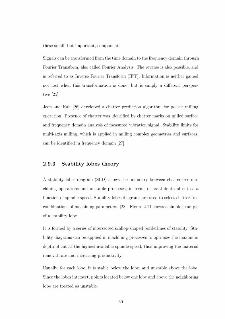
A stability lobes diagram (SLD) shows the boundary between chatter-free ma-
chining operations and unstable processes, in terms of axial depth of cut as a
function of spindle speed. Stability lobes diagrams are used to select chatter-free
combinations of machining parameters. [28]. Figure 2.11 shows a simple example
of a stability lobe
It is formed by a series of intersected scallop-shaped borderlines of stability. Sta-
bility diagrams can be applied in machining processes to optimize the maximum
depth of cut at the highest available spindle speed, thus improving the material
removal rate and increasing productivity.
Usually, for each lobe, it is stable below the lobe, and unstable above the lobe.
Since the lobes intersect, points located below one lobe and above the neighboring
lobe are treated as unstable.
30
Figure 2.11. Stability Lobe Diagram[28]
2.10 Tool path optimization
Optimization refers to a process of determining the best solution from among
possible solutions. In manufacturing, optimization can be carried out with various
technological goals such as:
• Achieving best possible surface quality
• Minimizing tool wear
• Achieving shortest machining time
• Minimizing machining costs
Optimizing cutting tool paths is one of the ways to achieve the global trend of
improving throughput and lowering cost of production in manufacturing indus-
try. Modern CAM softwares such as Mastercam R© provide up to eight tool path
strategies that can be used to machine a simple rectangular pocket, as shown in
Figure 2.12.
31

Figure 2.12. Screenshot of tool path strategies available for machininga rectangular pocket using Mastercam R©
These variety of tool path strategies leaves a wide room for improvement of tool
path efficiency. There exists a gap in the criteria that is used in selecting or
generating the tool path to be applied in machining a pocket. By evaluating the
quality and efficiency of the alternative solutions an optimal solution can be se-
lected. In optimization of milling tool path, factors such as cutting-tool geometry
and material, work piece material and geometry, machining operation and use of
coolants must be taken into account. Some of the approaches that have been
applied in optimizing tool paths include reduction of machining time, minimiza-
tion of cutting forces, modification of corner sections and avoiding redundant tool
movements and potential collisions.
Daneshmand et al [29] investigated the numerous tool paths available in two
common CAD/CAM softwares, CATIA R© and Mastercam R© so as to determine the
most suitable tool path. This was done for the roughening operation of machining
a gearbox model and a disc screen, using both end mill and ball-nosed tools.
They simulated the tool-path planning strategies according to the machining
32

time provided by the software. The accuracy of the operations verified the most
suitable tools path. Their research results indicated that for Mastercam R©, the
minimum machining time was achieved with zig-zag strategy when using end mill,
and spiral strategy when using ball-end tool. For CATIA R©, the back and forth
strategy gave the minimum machining time when using end mill and the inward
helical strategy when using ball-nose tool. They also found that machining time
changes when the geometry of the object being machined was altered.
Another approach that has been applied in selection of milling paths for complex
surfaces is minimizing of dimensional errors due to tool deflection, which was
presented by Lopez de Lacalle et al [30]. This resulted in an improvement on
the accuracy of milled surfaces. It was based on the calculation of the minimum
cutting force component, which was related to the tool deflection. In their first
suggestion, a general tool path direction was selected that minimized the mean
value of the tool deflection force on the surface. Based on this the CAM operator
could then produce a CNC program which lead to an accuracy improvement. The
second option was to create a grid of control points and select different milling
directions at each control point. Joining these points, the minimum force lines
were defined on the workpiece surface and used as the master guides for the tool
path programming of a complete surface. After applying these methods to 3-axis
milling the dimensional errors reduced from 30 mm to below 4 mm.
Choi and Cheung [31] proposed a method focused on avoiding redundant tool
movements and collisions in Multi-Material Layered Manufacturing (MMLM)
of heterogeneous prototypes. The approach facilitated control of MMLM and
increased the fabrication efficiency of complex objects by generating multi-tool
paths that avoid redundant tool movements and potential collisions. They used
a topological hierarchy-sorting algorithm to group complex multi-material con-
tours into groups connected by a parent-and-child relationship. The multi-tool
33

paths generated enabled sequential deposition of materials without redundant
tool movements. The build time was further reduced by another tool path plan-
ning algorithm that generated collision-free multi-tool paths to control the tools
that deposit materials concurrently.
Neural networks have also been applied in optimizing tool paths, as described
by Korosec and Kopac [32]. They demonstrated how with the help of artificial
neural network, the prediction of milling tool path strategies could be performed
in order to determine which tool path strategies or their sequence would yield the
best results, since any machining task may be carried out using different tool-
path strategies or sequences of various strategies. The result was that only one
of all possible applied strategies was optimal in terms of the desired technological
goal or aim. The study was based on production of car lights equipment by
the tool shop industry. Their technological aim was to achieve the best possible
surface quality of machined workpieces, which they verified by measuring surface
roughness.
Conventional tool paths can be modified and even additional tool paths appended
to the tool paths to achieve the optimal tool path. Hyun-Chul Kim [33] presented
an optimized tool path, which maintained Material Removal Rate (MRR) as
constant as possible so as to achieve constant cutting forces and to avoid chatter
vibrations. In his work additional tool path segments were appended to the basic
tool path obtained by geometric shape using a pixel-based simulation technique.
The algorithm was implemented for two-dimensional end milling operations, and
cutting tests were carried out by measuring spindle current, to reflect the state
of machining.
El-Midany et al [34] developed a feed rate-machining time model that took into
account machine acceleration and deceleration for automatically identifying the
most productive tool path pattern. The model was then used to compare the
34

total machining time for five common types of tool path patterns, namely, normal
zigzag, smooth zigzag, normal spiral, smooth spiral and fishtail spiral. The results
showed that the optimal tool path pattern was dependent on part geometry,
physical characteristic of cutting tool and cutting conditions.
Pateloup et al [35], proposed a pocketing tool path improvement method that
involved modification of the values of the corner radii in order to increase real
feed rate. This method checked the radial depth of cut variations along the tool
path. The computed tool path presented a smaller length and the machine tool
produced a higher average feed rate at the same time. Use of B-splines for tool
path computation was a notable improvement in this method, as compared to
the use of straight lines and arcs.
Choy et al [7] suggested a corner-looping-based tool path for pocket milling. The
basic pattern for the improved tool path was a conventional contour-parallel tool
path. In their research they appended bow-like additional segments to the corner
sections in the tool path such that corner material was removed progressively in
several passes, to prevent rise in cutting resistance. The proposed tool path was
implemented as an add-on user function in a CAD/CAM system.
Wang et. al. [36] proposed an integrated optimization of cutting parameters
and the generation of tool path in raster milling. In their work, they proposed a
methodology that optimized the cutting feed rate, the path interval, and the entry
distance in the feed direction simultaneously, in order to achieve the best surface
quality in a given machining time. This was achieved by implementing prediction
models for surface roughness and machining time in ultra precision raster milling.
The work improved surface quality without compromising efficiency of the milling
process.
35

Tool path optimization has also been done with a goal of improving energy ef-
ficiency of CNC machines. Li et. al. [37]. In this work, the authors developed
an energy consumption model. The model took into account the energy con-
sumption, which was the performance criteria, in optimization the tool path
connection. The simulated annealing and exhaustive algorithm were applied in
the optimization process. The model was was proven to be achieve an energy
efficient machining process.
In summary, models have been made to optimize specific tool paths such as zigzag
and contour parallel tool paths. Variations of the these tool paths have also been
developed such as the curvilinear tool paths currently applied in manufacture
of aerospace parts, which are neither straight nor curved. However, the CNC
machine operator still faces the challenge of generating the optimal tool path
from all the variations available in the CAM software. Production is still being
done using tool paths of which the operator has no way of knowing if they are
optimal. Models that have been developed so far consider only a single factor
such as speed, feedrate or depth of cut that would affect productivity, but neglect
dynamic factors such as cutting force and chatter vibration.
This work is therefore meant to create a way to predict dynamic factors, that is
machining time, cutting forces and chatter vibration at the point of selecting ma-
chining parameters. Pocket milling involves selecting of parameters that include
the tool path strategy whose impact is investigated in this study. The selection
of other parameters, that is, spindle speed, feedrate and depth of cut can then
be done with a predicted view of the cutting forces and chatter vibration.
36

CHAPTER 3
METHODOLOGY
3.1 Identification of cutting constants
The mechanistic approach of determining milling coefficients was applied to iden-
tify cutting constants. Experimental work was done on a vertical machining cen-
ter using high speed steel cutters. The workpiece material was Aluminium 7075-0.
For this preliminary experiments, one-tooth cutter was used to eliminate errors
due to uneven diameters at the different tool tips.
In this method, a set of milling experiments were conducted at different feed rates
but constant immersion angle and axial depth of cut. The average forces per tooth
period were then obtained from the measured data. The values for cutting forces
obtained experimentally were equated to the those derived analytically thus the
values of the various cutting constants were identified. These cutting forces are
independent of helix angle since material removed per tooth period is constant.
The setup shown in Figure 3.1 was used to measure instantaneous cutting forces.
Figure 3.1. Experimental setup for determination of baseline data.
37

3.2 Modelling of cutting force
In the static force model, each tooth of a helical end milling cutter is discretised
into a number of elements along the cutter axis. In milling process, the principal
forces acting on the cutting edge are Tangential (Ft,j), Radial (Fr,j) and Axial
(Fa,j) forces. These are shown in Fig. 3.2. Axial force is parallel to the tool axis.
Figure 3.2. Cutter modelling
Forces acting on a differential element of height dz in the axial direction, that is,
dFt,j, dFr,j and dFa,j, as explained in section 2.3, are expressed as
dFt,j(φ, z) = [Kt,fhj(φj(z)) +Kte]dz,
dFr,j(φ, z) = [Kr,fhj(φj(z)) +Kre]dz, (3.1)
dFa,j(φ, z) = [Ka,fhj(φj(z)) +Kae]dz,
where dz is the height of the differential element and hj is the static chip thickness
for the jth element at rotation angle φ. This chip thickness for a rigid system is
given by
hj(φ, z) = [ft sinφj(z)]g(φj), (3.2)
38

where ft is feed per tooth.
The total cutting force is calculated by summing up the elemental forces for
the entire part that is engaged with the workpiece. Cutting force is calculated
based on the undeformed chip thickness, cutting conditions and specific cutting
coefficients [16]. Kt, Kr and Ka are model coefficients in tangential, radial and
axial directions for the specific cutter-workpiece combination. The cutting forces
on tooth j in the x and y directions are obtained as
Fxj = −Ftj cos(φj)− Frj sin(φj)
Fyj = −Ftj sin(φj)− Frj cos(φj) (3.3)
where Ftj = Ktah(φj) and Frj = KrFtj.
Integration is then done along the whole axial depth to obtain the values of
differential forces, which are summed to obtain the cutting force values as in
Equation 3.4.
Fx =N−1∑j=0
Fxj(φj)
Fy =N−1∑j=0
Fyj(φj) (3.4)
where φj is the rotational position of tooth j and φj = φ + jφp and φp = 2πN
. φ
varies with time and φ = Ωt where Ω is the spindle angular speed in rad/s.
The model was simulated in MATLAB and is summarized in the flowchart shown
in Figure 3.3. The standard model inputs were as listed in Table 3.1.
39

Figure 3.3. Flowchart of milling force simulation
40

Table 3.1: Model inputs
Input parameter Value
Milling operation Up millingAxial depth(a) 2 mmNominal depth of cut(b) 2.4 mmFeedrate(f) 0.2 mm/toothSpindle speed(N) 325 rpmHelix angle (β) 30Number of teeth(nt) 2Cutter diameter(D) 8 mm
The cutter pitch angle φp for a cutter with nt teeth is given by Equation 3.5.
φp = (2π)/nt (3.5)
3.2.1 Cutter engagement boundaries
Of importance in the determination of cutting forces is the cutting phase which
means the cutter is engaged on the workpiece. Cutting forces occur only when the
cutter is within this engagement boundary, that is Fx(φ) = 0, Fy(φ) = 0, Fz(φ) =
0 when φst ≤ φ ≤ φex. The start and exit angle are illustrated in Figure 3.4.
a. Up milling b. Downmilling
Figure 3.4: Start and exit angles
41

The start or entry angle in up milling is φs = 0 while the exit angle depends on
the radius of the tool,r and the nominal depth of cut, b, and is given by
φe = cos−1(r − b
r). (3.6)
In down milling, the exit angle is φe = 180. The start angle is dependent on the
nominal depth of cut and the radius of the tool, and is given by
φs = 180− θ = 180− cos−1(r − b
r). (3.7)
The start and exit angle during a milling operation can be easily visualised in
the cutting force waveform, such as the one in Figure 3.5. The waveform is a
predicted waveform generated from the algorithm summarized in Figure 3.3.
Figure 3.5. Variation of cutting force with cutter rotation angle
42

3.3 Dynamic milling system model
In the dynamic force model, a predictive time domain model is presented for the
simulation and analysis of the dynamic cutting process and chatter in milling.
The instantaneous undeformed chip thickness is modelled to include the dynamic
modulations caused by the tool vibrations so that the dynamic regeneration effect
is taken into account as described by Altintas [38].
The governing equations for the dynamic milling system are given in Equation
3.8.
mxx+ cxx+ kxx =N−1∑j=0
Fxj(φj) = Fx(t),
myy + cyy + kyy =N−1∑j=0
Fyj(φj) = Fy(t), (3.8)
where m is the mass, c is the damping constant, and k is the spring constant. This
model was implemented in MATLAB R©. The dynamic milling system cannot be
expressed as simple analytical functions and the dynamic differential equations
which represent the system cannot be solved analytically since the system is non-
linear. Numerical methods are thus used to solve these differential equations.
The solution is an approximate solution, in which the continuous time variable t
is replaced by a discrete time variable, and the differential equations are solved
in steps, with an increment of dt. The solution starts at known initial conditions.
The model for the dynamic regenerative chip thickness is illustrated in Figure 3.6
The static undeformed chip thickness is determined from the feed per tooth as
43

Figure 3.6. Model for dynamic regenerative chip thickness
h = g(φj)[f sinφj], (3.9)
where g(φj) is a unit step function that determines whether the tooth is in cut
or out of cut.
In the dynamic milling process the undeformed chip thickness is comprised of two
parts, a static part, h, and a dynamic component caused by the present tooth
period (inner modulation) vj, and previous tooth period (outer modulation) vjo.
The static part does not contribute to the dynamic chip load, hence the dynamic
undeformed chip thickness for tooth j at an angular position φj is calculated as
hd(φj) = [∆x sin(φj) + ∆y cos(φj)]g(φj), (3.10)
where ∆x = x−x0, ∆y = y−y0 and (x, y) and (x0, y0) are the dynamic displace-
ments at the present and previous tooth periods respectively. The rotation angle
varies with time, φ(t) = Ωt where Ω is the spindle angular speed in rad/s. The
tooth passing frequency ω = ntΩ and the tooth period T = 2πω
, where nt is the
number of teeth on the cutter.
The dynamic cutting forces on tooth j in the x and y directions are obtained as
44

Fxj = −Ftj cos(φj)− Frj sin(φj)
Fyj = −Ftj sin(φj)− Frj cos(φj) (3.11)
where Ftj = Ktah(φj) and Frj = KrFtj, where a is axial depth of cut.
The total dynamic milling forces for all teeth are given by
Fx =M−1∑j=0
Fxj(φj),
Fy =M−1∑j=0
Fyj(φj), (3.12)
where φj is the rotational position of tooth j and is given by φj = φ + jφp and
φp = 2πnt
. φ varies with time and is given by φ = Ωt where Ω is the spindle angular
speed in rad/s.
The MATLAB R©model is designed based on three main blocks namely; milling
forces, milling kinematics, and system dynamics. The milling kinematics in-
volve the calculation of the chip thickness. The concept of discretizing the
tool/workpiece model is employed in chip thickness and cutting force compu-
tation.
The model inputs include:
1. Tool geometry parameters: number of teeth, tool diameter, helix angle,
flank length
2. Cutting parameters: spindle speed, feed per tooth, depth of cut, cutting
45

coefficients
3. Dynamic parameters: natural frequency, mass, stiffness and damping coef-
ficient for each mode of vibration
4. Simulation parameters: number of cycles, iterations per cycle and number
of axial layers
This work proposes that the ratio of the predicted maximum dynamic cutting
force, max (Fd), to the predicted maximum static cutting force, max (Fs), be
used as a criterion for the chatter stability, as given in Equation 3.13. These
maximum values are selected from a period of several tool revolutions. From
these values, a force ratio, ρ is defined as
ρ =max(Fd)
max(Fs), (3.13)
where Fd is the cutting force predicted using dynamic cutting force model which
takes into account the regenerative effect on the undeformed chip thickness, and
Fs is the cutting force predicted using the static cutting force model. This ratio
is used to determine whether there is chatter or not.
The model outputs are the instantaneous static and dynamic cutting forces in x
and y directions, the maximum static and dynamic cutting forces and the chatter
value.
3.4 Experimental work
In this section experimental procedure to verify theoretical models developed in
sections 3.2 and 3.3 is outlined.
46

3.4.1 Tool path generation and simulation
MasterCAM CAD/CAM software was used in design of parts and generation of
tool paths for the various pockets. It was also used to simulate and obtain the
machining times for the various operations. To obtain the machining times when
using the zigzag (direction-parallel), parallel spiral (contour parallel) and smooth
spiral tool paths shown in Figure 3.10, simulation was done for the machining of
a rectangular pocket measuring 30 mm by 20 mm to a depth of 10 mm.
Figure 3.7. (a) Parallel spiral tool path (b) Zigzag tool path (c) Truespiral tool path
Zigzag tool path: It is a direction-parallel tool path where the tool cuts both
in the forward and backward direction. It results in less tool retractions than the
one way tool path but also presents sharp corner cutting.
Parallel spiral: The tool cuts in a spiral motion following the pocket contour.
The tool has one start and one finish position for every depth cut. It is charac-
47

terized by sharp corners which may necessitate the use of a smaller diameter tool
for finishing the corners.
True spiral: This tool path is generally similar to the parallel spiral tool path,
however the path does not follow the pocket contour but follows a true spiral
path. Sharp direction changes are only encountered at the start or end of the
depth cut depending on whether an inward or outward spiral was applied.
The difference in the machining times is illustrated in Figure 3.8. The machining
times are stored in MS Excel document for ease of reading into MATLAB R© by
optimization algorithm.
Figure 3.8. Machining times when using different tool path strategies(Rectangular pocket, 30 mm by 20 mm by 10 mm)
48

3.4.2 Fixture and workpiece design and preparation
To be able to mount the workpiece securely onto the dynamometer, a fixture was
designed and machined. The design was such that there was a provision to fasten
the workpiece onto the fixture and also secure the fixture-workpiece assembly
onto the dynamometer. The workpiece was fastened onto fixture using four M12
socket bolts and the fixture-workpiece assembly was secured onto dynamometer
using six M10 socket bolts.
3.4.3 Dynamometer calibration
The setup used in dynamometer calibration is illustrated in Figure 3.9.
Figure 3.9. Experimental setup for dynamometer calibration
Loads of known weights were applied along the x and y direction one at a time
and the readings in all 3 components were recorded. It was observed that for each
direction loaded there was interaction in all 3 components which was compensated
for by the use of calibration equations. Calibration curves were obtained for 3-
component cutting force dynamometer, from which the force components for all
directions were derived.
49
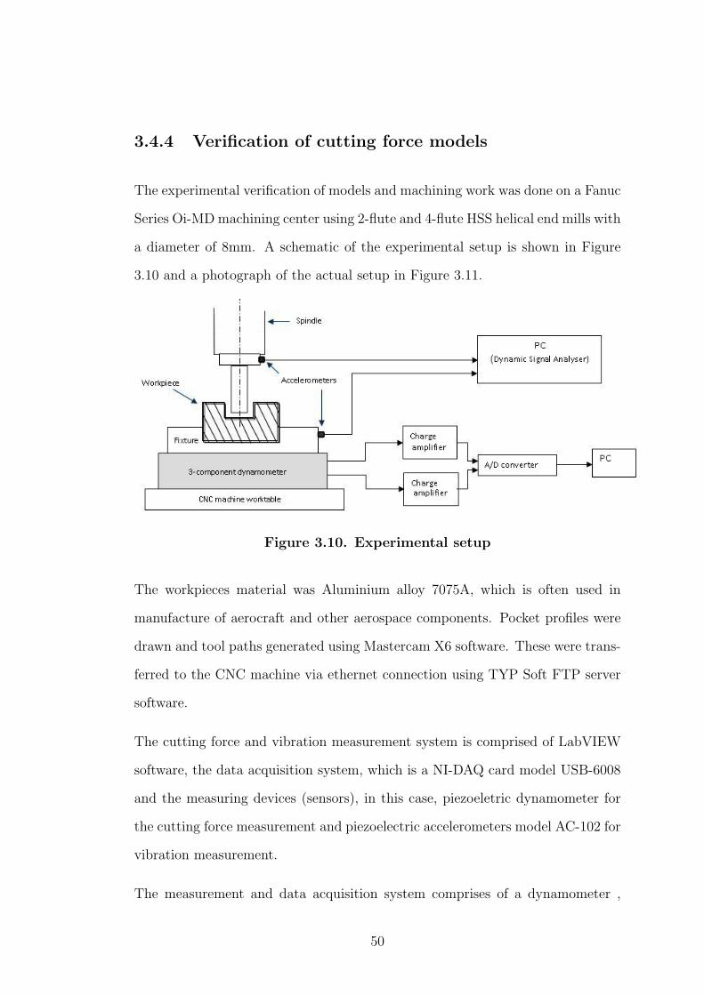
3.4.4 Verification of cutting force models
The experimental verification of models and machining work was done on a Fanuc
Series Oi-MD machining center using 2-flute and 4-flute HSS helical end mills with
a diameter of 8mm. A schematic of the experimental setup is shown in Figure
3.10 and a photograph of the actual setup in Figure 3.11.
Figure 3.10. Experimental setup
The workpieces material was Aluminium alloy 7075A, which is often used in
manufacture of aerocraft and other aerospace components. Pocket profiles were
drawn and tool paths generated using Mastercam X6 software. These were trans-
ferred to the CNC machine via ethernet connection using TYP Soft FTP server
software.
The cutting force and vibration measurement system is comprised of LabVIEW
software, the data acquisition system, which is a NI-DAQ card model USB-6008
and the measuring devices (sensors), in this case, piezoeletric dynamometer for
the cutting force measurement and piezoelectric accelerometers model AC-102 for
vibration measurement.
The measurement and data acquisition system comprises of a dynamometer ,
50

two accelerometers model AC-102, three charge amplifiers, an NI-DAQ card USB
6008, LabView software and the relevant connecting cables. As the tool cuts
through the workpiece, the force is transmitted to the dynamometer. Cutting
force measurements were taken using a table mounted dynamometer during ma-
chining. The dynamometer measures the cutting force in the x, y and z axes.
The dynamometer is clamped between the workpiece and the table. The fixture
was used to mount the workpiece on the dynamometer. When the piezoelectric
quartz in the dynamometer is strained an electric charge is generated. The elec-
tric charge is then transmitted to the charge amplifiers through the connecting
cable where it is amplified. The voltage output by amplifier corresponds to the
cutting force based on the parameters set in the charge amplifier.
The accelerometers were mounted on the workpiece to measure vibration in the
x and y directions, using threaded studs which provided a firm mounting.
The DAQ card transmits the voltage signals from the charge amplifiers and the
accelerometers into a PC via USB slot so that the LabVIEW software is able to
read and utilize the data.
3.5 Chatter stability criterion
A set of experiments and signal analysis were carried out in order to set a chatter
value. This value is the ratio of maximum predicted cutting force to maximum
predicted static cutting force. Since the measured cutting force is in agreement
with predicted dynamic cutting force, the chatter element allows chatter predic-
tion without the need for experiments.
Chatter vibration was not clearly evident in the cutting force waveforms, since the
workpiece material is soft. Therefore, the vibration signals from the accelerome-
51

Figure 3.11. Photograph of the experimental setup
ters were analyzed in the frequency domain. In the frequency spectrum, chatter
is present when there are large peaks near the natural frequency of the system.
A stable cut only has peaks due to resonance at natural frequency and tooth
passing frequency in the frequency spectrum. In the frequency spectrum for an
unstable cut other frequency peaks are observed within the range of 20-27 Hz,
which are the vibration frequencies.
A digital low-pass filter was applied to the accelerometer data signal to minimize
high frequency noise signal which was observed. The data processing was done
in MATLAB R©.
For example in a pocket milling test at spindle speed 450 rpm, axial depth of cut
1 mm, feedrate 0.08 mm/tooth using a cutter of diameter 8 mm, the maximum
static and dynamic forces were found to be 16.48 N and 19.03 N respectively,
giving a ratio ρ of 1.154.
Fdy max = −19.03 N
52
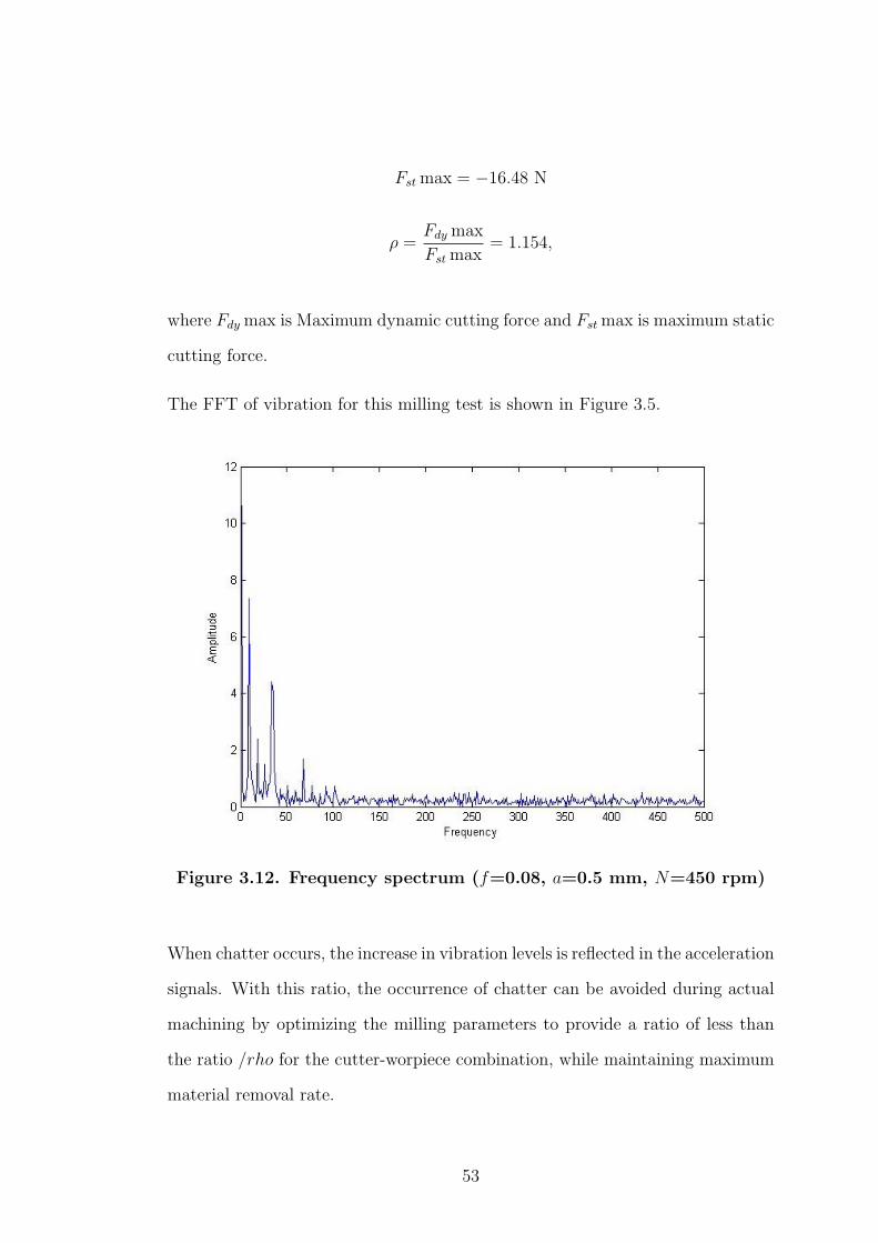
Fst max = −16.48 N
ρ =Fdy max
Fst max= 1.154,
where Fdy max is Maximum dynamic cutting force and Fst max is maximum static
cutting force.
The FFT of vibration for this milling test is shown in Figure 3.5.
Figure 3.12. Frequency spectrum (f=0.08, a=0.5 mm, N=450 rpm)
When chatter occurs, the increase in vibration levels is reflected in the acceleration
signals. With this ratio, the occurrence of chatter can be avoided during actual
machining by optimizing the milling parameters to provide a ratio of less than
the ratio /rho for the cutter-worpiece combination, while maintaining maximum
material removal rate.
53

3.6 Optimization of pocket milling parameters
The goal of optimization in this research is to select process parameters that
ensure minimal cutting forces, ensure chatter vibration does not occur, while
taking the shortest time possible to machine a pocket. Being a multi-objective
optimization problem, the weighted sum optimization approach was applied. This
method scales the set of objectives into a single objective by multiplying each
objective with its respective weight [39]. This is formulated as
Ai =n∑
j=1
wiai (3.14)
where a1 is force ratio below 1.238, a2 is minimum cutting force and a3 is minimum
machining time, and w1 = 5 for a1, and w1 = 3 for a2, and w1 = 2 for a3.
The static and dynamic force models are used to determine the prediction of
chatter vibration occurrence. Mastercam R© software is used to simulate and store
machining times, which are read by optimization algorithm. The parameters
under study are feedrate and axial depth of cut. The algorithm allows off-line
optimization of the machining parameters especially the feedrate based on the
predicted cutting force, chatter value and machining time. MATLAB R© software
was used to develop the optimization algorithm whose summary is shown in
Figure 3.6.
The integration of the models developed in the simulation of the pocket milling
process including the tool path strategy was not achieved due to limitations in
the softwares used, that is MATLAB R© and Mastercam R©. Such work done from a
single platform such as Matlab is possible but could not be accomplished within
the research period. The development of a platform for simulation of the milling
process with consideration of the tool path strategy is thus a potential research
54

area.
Figure 3.13. Optimization flowchart
55

CHAPTER 4
RESULTS AND DISCUSSION
In this chapter, results on cutting constants determined using the mechanistic ap-
proach are presented. Also, experimental results verifying the developed models,
and results on the effects of pocket milling parameters on milling forces and chat-
ter vibration are presented and discussed. The parameters investigated include
axial depth of cut, feedrate and tool path strategy.
4.1 Determination of cutting constants
Figure 4.1 shows a waveform of measured instantaneous cutting force.
Figure 4.1. Force waveforms for side milling (f=0.2 mm/t, N=705min−1,a= 5mm,nt=1)
From this kind of waveform, the average cutting forces per tooth period for the
different feedrates were obtained as given in Table4.1. These values are applied
in Equation 2.18 and the cutting and edge force coefficients obtained are given
in Table 4.2.
56

Table 4.1: Average cutting forces per tooth period
Feedrate F x(N) F y(N) F z(N)0.1 -19.5 72.5 -21.60.2 -23.2 135.4 -30.20.3 -34.5 160.2 -35.80.4 -36.2 224.1 -41.4
Table 4.2: Cutting and edge coefficients
Constant Symbol ValueTangential cutting coefficient Ktc 198.4Radial cutting coefficient Krc 90.63Axial cutting coefficient Kac 890Tangential edge coeffcient Kte 30.86Radial edge coefficient Kre 17.96Axial edge coefficient Kae -7.89
4.2 Verification of static and dynamic cutting
force models
Experimental tests were carried out to verify the static and dynamic force models
that were developed. For this tests, the standard milling parameters were as in
Table4.3.
Table 4.3: Standard milling parameters
Parameter ValueNumber of teeth 4Cutter overhang length 30 mmAxial depth of cut 1 mmFeedrate 0.08 mm/toothSpindle speed 450rpmTool path strategy Parallel spiral
Figure 4.2 shows the waveforms of instantaneous cutting forces from measured
and predicted forces in x and y directions, respectively.
It can be seen from this waveforms that the predicted forces are generally in good
57

(a) Force in x direction
(b) Force in y direction
Figure 4.2. Waveforms for predicted and measured cutting forces
agreement with experimental results. The measured signal has noise disturbances
unlike both static and dynamic models, which is due to the engagement and
disengagement of the cutting tool from the workpiece. This noise signal is more
pronounced in the x direction, which was the feed direction for this test. This is
because the greatest tool displacements occur in the feed direction. The dynamic
model is found to be more accurate than the frequently used static model. The
average percentage error when predicting using static model was found to be
16.86% while the average percentage error when using dynamic force model was
58

7.98% as obtained in Table 4.4. The dynamic model is thus more reliable.
Table 4.4: Table of comparison for measured and predicted forces
Test
Average ex-perimentalresultantforce(N)
Static modelaverage re-sultant force
Percentageerror
Dynamicmodel aver-age resultantforce
Percentageerror
1 14.27 15.90 11.46 12.94 9.322 35.46 38.72 9.20 37.95 7.023 51.52 63.12 22.52 57.38 11.384 91.38 96.76 5.89 96.26 5.345 44.30 49.85 12.54 43.15 2.606 74.26 87.41 17.71 73.26 1.357 87.93 96.76 10.04 80.06 8.958 23.02 24.41 6.06 24.55 6.669 58.84 68.54 16.48 65.21 10.8310 53.39 59.80 12.00 55.17 3.3411 61.56 81.03 31.63 65.24 5.9912 36.79 46.14 25.43 31.91 13.2613 35.96 41.28 14.82 39.17 8.9314 100.07 111.05 10.97 101.25 1.1815 157.25 170.14 8.20 126.21 19.7416 132.73 136.66 2.96 133.03 0.23
4.3 Effect of depth of cut on cutting force
Test were done at varying depths of cut, with all other parameters maintained at
standard values given in Table 4.3. The data obtained is given in Table 4.5. It was
observed that cutting forces increased with increase in depth of cut and decreased
with decrease in depth of cut, as shown in Figure 4.3 in x and y direction. As axial
depth of cut increases, the area of contact of the tool with the workpiece, and
the volume of material removed also increase, which leads to increase in cutting
force. The predicted values were in good agreement with the measured values.
59

Depth ofcut (mm)
PredictedFx (N)
PredictedFy (N)
MeasuredFx (N)
MeasuredFy (N)
0.5 -11.91 16.26 -14.30 18.221 -23.83 32.53 -26.21 32.201.5 -35.74 48.79 -35.74 49.772 -47.65 65.06 -50.04 67.01
Table 4.5: Variation of cutting force with depth of cut
Figure 4.3. Variation of cutting force with depth of cut
4.4 Effect of feedrate on cutting force
Test were done at varying feedrates, with all other parameters maintained at
standard values given in Table 4.3. The data obtained is given in Table 4.6.
Cutting forces increase with increase in feedrate and decrease with decrease in
feedrate, as shown in Figure 4.4. Higher feedrate increases the material remove
rate (MRR) which results in higher cutting forces. Also with high feedrate the
metal may be pushed instead of being cut. This also results in higher cutting
force and higher temperature. The predicted values were in good agreement with
the measured values.
60

Feedrate(mm/tooth)
PredictedFx (N)
PredictedFy (N)
MeasuredFx (N)
MeasuredFy (N)
0.02 -14.68 11.05 -14.97 11.270.08 -23.83 32.53 -21.69 29.600.14 -31.65 43.68 -28.09 39.560.2 -39.73 59.47 -44.50 66.61
Table 4.6: Variation of cutting force with feedrate
Figure 4.4. Variation of cutting force with feedrate
4.5 Cutting force waveforms for different tool
path strategies
The cutting force waveforms observed when milling using parallel spiral tool path,
zigzag tool path and true spiral tool path are shown in Figure 4.5. The measure-
ment time period is one complete depth pass. The cutter parameters were D = 8
mm, nt = 4, overhang length=30 mm. The milling parameters for all three tests
were: a = 0.5 mm, f = 0.07 mm/tooth, N = 500 rpm.
The peak-to-peak force when milling using true spiral tool path is 125.26 N in
the x direction and 143.60 N in the y direction. When milling using parallel
spiral tool path the peak-to-peak force in x direction is 203.72 N and 206.79 N
61

in the y direction. The highest peak-to-peak forces occur when using zigzag tool
path with force in x direction being 173.17 N in x direction and 254.73 N in y
direction. The highest force values are measured at corner sections of the milling
path, where there is larger tool engagement into the workpiece.
From the analysis, it was observed that the tool path strategy used had a signif-
icant effect on the magnitude of cutting forces that the tool experiences. Rapid
direction changes caused a rise in cutting forces, due to the variation of the extent
of radial engagement of the cutting tool as its direction changes. At the corner
sections seen in zigzag and parallel spiral tool path, the maximum radial engage-
ment of the tool occurs. The true spiral tool path, where the tool does not make
sharp direction changes has the least average cutting forces in both directions.
62

(a) Parallel spiral
(b) Zig-zag
(c) True spiral
Figure 4.5. Cutting force waveforms for various tool path strategies
63

4.6 Effect of tool path strategy on cycle time
Milling tests were done to machine two pockets, a square of length 30 mm and a
rectangular pocket measuring 40 mm by 30 mm. The machining time for milling
the rectangular pocket using parallel spiral tool path was 670 seconds, with zigzag
tool path was 636 seconds while using true spiral tool path was 874 seconds. The
machining time for milling the square pocket using parallel spiral tool path was
338 seconds, with zigzag tool path was 301 seconds while using true spiral tool
path was 291 seconds as shown in Figure 4.6.
Figure 4.6. Cycle times for different tool path strategies
The suitability of a tool path strategy in terms of cycle time is dependent on
the profile of the pocket. For the rectangular pocket, zigzag tool path strategy
took the shortest to machine the pocket while true spiral took the longest time.
For the square pocket, true spiral tool path strategy took the shortest time while
parallel spiral tool path took the longest time.
64

4.7 Determination of chatter boundary
In order to determine the force ratio, a set of experiments were conducted with
depth of cut, feedrate and spindle speed being varied. The vibration signals from
the accelerometers were analyzed in the frequency domain. In the frequency
spectrum, chatter is present when there are large peaks near the natural frequency
of the system. A stable cut only has peaks due to natural frequency and tooth
passing frequency in the frequency spectrum. Tests with this kind of spectrum
are plotted as in Figure 4.7.
In the frequency spectrum for an unstable cut , plotted as , other frequency
peaks are observed within the range of 20-27Hz, which are the vibration frequen-
cies. This can be seen in Fig. 10(d). Test for which there are other small peaks
which cannot be concluded to be chatter, such as in Fig. 10(c) are plotted as .
Table 4.7 shows the values of ρ obtained for 20 tests. These data was plotted as
shown in Figure 4.7, from which a boundary was observed at 1.238.
Test Force ratio Vibration1 1.114 no2 1.280 yes3 1.209 slight4 1.326 yes5 1.165 slight6 1.138 no7 1.127 no8 1.154 no9 1.248 yes10 1.223 slight11 1.105 no12 0.992 no13 1.249 yes14 1.302 yes15 1.042 no16 1.273 yes17 1.626 yes18 1.238 yes19 1.158 slight20 1.120 no
Table 4.7: Table of force ratios
65

Figure 4.7. Plot of chatter values
During milling, parameters can be selected and applied in the chatter predic-
tion model, where the ratio of maximum dynamic cutting force to maximum
static cutting force is evaluated. For the cutter-workpiece combination used in
this experiment, a ratio equal to or above 1.238 means that chatter vibration is
expected to occur.This force ratio was successfully applied to predict, and thus
avoid, occurrence of chatter vibrations.
4.8 Effect of tool path strategy on chatter vi-
bration
The cutting force and vibration data measured in time domain was transformed
into frequency domain using Fast Fourier Transform (FFT) method. This trans-
formation was done in order to identify occurrence of chatter vibrations during
66

milling. From the FFT analysis it is observed that the forces are harmonic waves.
The dominant peak frequency occurred at 30 Hz, which is the tooth passing fre-
quency. Harmonics of the fundamental frequency which occur at integral mul-
tiples of the fundamental frequency are also observed in some experiments. A
peak due to the spindle frequency was also observed at 7.5Hz. The variation in
magnitudes of fundamental frequency from the performance of an FFT analysis
can be used as an indicator to detect the variations of the cutting force [40].
FFT analysis was done on force measured when machining a pocket at standard
machining parameters given in Table 4.3 using parallel spiral tool path, zigzag
tool path, and true spiral tool paths. The chatter prediction model gives a chatter
value of 0.736, hence chatter vibration was not predicted to occur. The frequency
spectrum of the measured forces is shown in Figure 5.1. There was no chatter for
any of the tool path strategies used. The tooth passing frequency for both tests
is 30 Hz, which is observed as the fundamental frequency in all three tests.
Since standard parameters did not present chatter vibration, the feedrate was
increased to 0.125 while all other parameters were maintained. This gave a force
ratio of 1.248, hence chatter vibration was predicted to occur. The FFT plots are
shown in Figure 4.8. The tooth passing frequency for both tests is 30 Hz, which
is observed as the fundamental frequency in all three tests.
From the FFT analysis, chatter vibration occurred during machining with all
three tool path strategies, as explained in Section 4.5. The tool path strategy was
not observed to affect the occurrence or lack of chatter vibration from the FFT
spectrum of vibration signal. However, the RMS of vibration acceleration was
observed to vary slightly with similar milling parameters but different tool path
strategy. This is due to the effect of sudden direction changes during machining
of corners in parallel spiral and zigzag tool paths.
67

The vibrations had the higher RMS when using parallel spiral tool path and
were not fully developed when using true spiral tool path. Force variations only
occurred at the end of the machining cycle for true spiral tool path, when the
tool encountered corner cutting.
4.9 Variation of vibration with feedrate
Pocket milling tests were carried out at standard parameters given in Table 4.3,
except feedrate which was varied of between 0.05 mm/tooth and 1.11 mm/tooth.
The frequency spectrum of the vibration measurements were analyzed and the
results compared. The severity of vibration is observed from the height of the
peaks at the various frequencies. At a high feedrate of 1.11 mm/tooth, the
dominant frequency shifts to the vibration frequency observed between 22-25 Hz
as seen in Figure 4.9. This is as a result of increased load on the teeth of the
cutter at higher feedrates, which is also transmitted to the workpiece.
In this chapter, the variation of machining time with various tool path strategies
was presented and discussed. The zigzag tool path strategy was found to have
the least machining time for the rectangular pocket profile while the true spiral
tool path was found to present the least machining time for a rectangular pocket.
68

(a) Parallel spiral:no chatter vibration
(b) Zigzag: no chatter vibration
(c) True spiral: no chatter vibration
Figure 4.8. Effect of tool path strategy on chatter occurrence
69
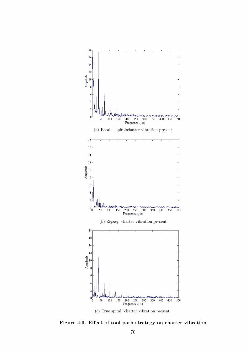
(a) Parallel spiral:chatter vibration present
(b) Zigzag: chatter vibration present
(c) True spiral: chatter vibration present
Figure 4.9. Effect of tool path strategy on chatter vibration
70

(a) 0.05 mm/tooth
(b) 0.83 mm/tooth
(c) 1.11 mm/tooth
Figure 4.10. Frequency analysis of vibration at different feedrates
71

CHAPTER 5
CONCLUSION AND RECOMMENDATIONS
5.1 Conclusion
In this study, static and dynamic force models for pocket milling were devel-
oped and validated. The models developed were tested at various depths of cut,
feedrate and using various tool path strategies.
These models were applied to predict chatter vibrations for the pocket milling
process. A chatter indicator defined as the ratio of dynamic force to static force
was validated through experimental work. It was established that for the ma-
chining of aluminium alloy 7075 using the HSS cutting tool this force ratio is
1.238.
An optimization control algorithm implemented in MATLAB R© was developed to
establish the optimal combination of parameters for milling of a pocket. With
a given set of milling parameters, the occurrence of chatter could be predicted
and hence avoided by adjusting the depth of cut and feedrate. The depth of
cut, feedrate and tool path strategy on the occurrence of chatter vibration was
also investigated. It was not possible to change the tool path strategy within
the optimization algorithm due to incompatibility between the MasterCAM R©
software and MATLAB R©. The algorithm was verified using experiments and was
found to be effective in ensuring chatter avoidance during actual milling.
72

5.2 Recommendations
Dynamics and stability modelling of milling process can influence various indus-
trial applications such as aerospace, automotive, die and mould, toolings, robots,
precision machining. From this study the following are recommendations towards
improvement in this area:
1. Incorporation of force and chatter prediction model in tool path generation
during pocket milling, to enable change of small sections of tool path to
suit the pocket profile. This is more for pockets with complex profiles.
2. The models developed cannot accurately predict the forces in corner cutting
during pocket milling. An adaptive controller should thus be developed that
can prevent the sharp rises in cutting force in such conditions.
73

REFERENCES
[1] D. M. Sukru, Mechanics and Dynamics of Serrated End Mills. PhD thesis,
University of British Columbia, 2003.
[2] B. W. Ikua, H. Tanaka, O. Fumio, and S. Satoshi, “Prediction of cutting
forces and machining error in ball end milling of curved surfaces-I Theoretical
analysis,” Journal of International Society for Precision Engineering and
Nanotechnology, vol. 25, 2002.
[3] M. Held, On the Computational Geometry of Pocket Machining. Springer
Science-Verlag, 1991.
[4] T. R. Kramer, “Pocket Milling with Tool Engagement Detection,” Journal
of Manufacturing Systems, vol. 11, pp. 114–123, 1992.
[5] G. Quintana and J. Ciurana, “Chatter in machining processes: A review,”
International Journal of Machine Tools and Manufacture, vol. 51, pp. 363–
376, may 2011.
[6] S. Fishwick and W. Tobias, “A theory of Regenerative Chatter,” The
Engineer-London, 1958.
[7] H. S. Choy and K. W. Chan, “A corner-looping based tool path for pocket
milling,” Computer-Aided Design, vol. 35, pp. 155–166, 2001.
[8] S. Park and B. Choi, “Tool-path planning for direction-parallel area milling,”
Computer-Aided Design, vol. 32, no. 1, pp. 17–25, 2000.
[9] A. E. M., M. Held, and C. L. Smith, “Optimization problems related to
zigzag pocket machining,” Algorithmica, vol. 26, no. 2, pp. 197–236, 2000.
74

[10] Advanced Robotic Technology, “Optimum tool path strategies reduce pro-
duction times,” 2011.
[11] P. N. Rao, Manufacturing Technology: Metal Cutting and Machine Tools.
Tata McGraw-Hill Plublishing Company Limited, 2 ed., 2009.
[12] B. W. Ikua, H. Tanaka, F. Obata, S. Sakamoto, T. Kishi, and T. Ishii,
“Prediction of cutting forces and machining error in ball end milling of curved
surfaces -II experimental verification,” Precision Engineering, vol. 26, no. 1,
pp. 69–82, 2002.
[13] J. G. Njiri, Optimization of machining process for freeform surfaces using an
intelligent adaptive controller (M. Sc. Thesis). 2010.
[14] J.-W. Dang, W.-H. Zhang, Y. Yang, and M. Wan, “Cutting force model-
ing for flat end milling including bottom edge cutting effect,” International
Journal of Machine Tools and Manufacture, vol. 50, no. 11, pp. 986–997,
2010.
[15] J. J. Wang, “Convolution Analysis of Milling Force Pulsation,” Journal of
Engineering for Industry, vol. 116, no. 25, 1994.
[16] O. Omar, T. El-Wardany, E. Ng, and M. Elbestawi, “An improved cutting
force and surface topography prediction model in end milling,” International
Journal of Machine Tools and Manufacture, vol. 47, pp. 1263–1275, jun 2007.
[17] W. Kline, R. Devor, and J. Lindberg, “The prediction of cutting forces in end
milling with application of cornering cuts,” International Journal of Machine
Tool Design and Research, vol. 22, no. 1, p. 722, 1982.
[18] Y. Altintas, Manufacturing Automation: Metal Cutting Mechanics, Machine
Tool Vibrations, and CNC Design. Cambridge University Press, 2012.
75

[19] E. Budak, Y. Altintas, and E. Armarego, “Prediction of milling force coef-
ficients from orthogonal cutting data.,” Journal of Manufacturing Science
and Engineering, vol. 118, no. 2, pp. 216–224, 1996.
[20] R. Butt, Introduction to Numerical Analysis Using MATLAB. Jones and
Bartlett Publishers, 2009.
[21] C. W. de Silva, Vibration and Shock Handbook. CRC Press, 2005.
[22] J. Tlusty and F. Ismail, “Basic non-linearity in machine chatter,” Annals of
CIRP, vol. 30, no. 1, pp. 21–25, 1981.
[23] J. Tlusty and P. Macneil, “Dynamics of cutting forces in end milling,” Annals
of the CIRP, vol. 24, pp. 21–25, 1975.
[24] J. H. Ko and Y. Altintas, “Time domain model of plunge milling operation,”
International Journal of Machine Tools and Manufacture, vol. 47, no. 9,
2007.
[25] R. L. Allen and D. W. Mills, Signal Analysis: Time, Frequency, Scale, and
Structure. John Wiley & Sons, 2004.
[26] J. H. Ko and K. C. Shaw, “Chatter prediction based on frequency domain
solution in CNC pocket milling,” International Journal of Precision Engi-
neering and Manufacturing, vol. 10, no. 4, pp. 19–25, 2009.
[27] L. T. Taner, S. Matej, and K. Jan, “Integrated simulation system for 5-
axis milling cycles,” in 15th C IRP Conference on Modelling of Machining
Operations, 2015.
[28] P. Palpadian, R. V. Prabhu, and B. S. Satish, “Stability Lobe Diagram for
High Speed Machining Process:Comparison of Experimental and Analyti-
cal Methods A Review,” International Journal of Innovative Research in
Science, Engineering and Technology, vol. 2, no. 3, 2013.
76

[29] S. Daneshmand, M. M. Abdolhosseini, and C. Aghanajafi, “Investigating the
Optimal Tool Path Strategies Based on Machining Time in CAD-CAM,”
Australian Journal of Basic and Applied Sciences, vol. 5, no. 12, pp. 2320–
2326, 2011.
[30] L. Lopez de Lacalle, A. Lamikiz, J. Sanchez, and M. Salgado, “Toolpath
selection based on the minimum deflection cutting forces in the programming
of complex surfaces milling,” International Journal of Machine Tools and
Manufacture, vol. 47, no. 2, pp. 388–400, 2007.
[31] S. Choi and H. Cheung, “A topological hierarchy based approach to tool
path planning for multi-material layered manufacturing,” Computer-Aided
Design, vol. 38, pp. 143–156, 2006.
[32] M. Korosec and J. Kopac, “Neural Network Based Selection of Optimal Tool
- Path in Free Form Surface Machining,” vol. 1, no. December, 2007.
[33] H.-C. Kim, “Tool path modification for optimized pocket milling,” Interna-
tional Journal of Production Research, vol. 45, no. 24, pp. 5715–5729, 2007.
[34] T. El-midany, H. Tawfik, and A. Elkeran, “Tool path pattern comparison:
Contour parallel with Direction-parallel,” in International Conference on
Geometric Modeling and Imaging-New Trends, 2006.
[35] M. Bouard, V. Pateloup, and P. Armand, “Pocketing toolpath computa-
tion using an optimization method,” Computer-Aided Design, vol. 43, no. 9,
pp. 1099–1109, 2011.
[36] S. J. Wang, S. To, X. Chen, X. D. Chen, and X. B. Ouyang, “An integrated
optimization of cutting parameters and tool path generation in ultrapreci-
sion raster milling,” The International Journal of Advanced Manufacturing
Technology, vol. 75, no. 9, 2014.
77

[37] X. Li, Q. Wang, J. Zhang, and J. Liu, “Tool path optimization for energy
efficient machining using exhaustive and simulated annealing,” in 2016 Sixth
International Conference on Information Science and Technology, 2016.
[38] Y. Altintas, Manufacturing Automation: Metal Cutting Mechanics, Machine
Tool Vibrations, and CNC Design. Cambridge University Press, 2000.
[39] M. Gen and R. Cheng, Genetic Algorithm and Engineering Optimization.
John Wiley & Sons, 2000.
[40] Y. Wang, X. Cui, H. Xu, and K. Jiang, “Cutting force analysis in reaming
of ZL102 aluminium cast alloys by PCD reamer,” International Journal of
Advanced Manufacturing Technology, vol. 67, pp. 1509–1516, 2013.
78

APPENDIX A
Instrument calibration
(a) Loading in x direction
(b) Loading in y axis
(c) Loading in z axis
Figure A.1: Dynamometer calibration curves
The set of simultaneous equations in Equation A.1 is obtained.
79

Rx = 0.357× 10⁻³Fx − 0.044× 10⁻³Fy − 0.020× 10⁻³Fz
Ry = 0.477× 10⁻³Fx + 0.010× 10⁻³Fy − 0.028× 10⁻³Fz (A.1)
Rz = 0.539× 10⁻³Fx + 0.029× 10⁻³Fy + 0.011× 10⁻³Fz
From this set of equations the force components in x, y and z directions are
calculated using Equation A.2.
Fx = 272.7Rx − 4.503Ry + 2.253Rz
Fy = −1.411Rx + 317.5Ry + 2.691Rz (A.2)
Fz = −2.712Rx − 1.825Ry + 360.6Rz
80

APPENDIX B
Matlab simulation of milling force
a=480; %(mm)axial depth
%b= %radial depth
c=0.1; %mm/tooth feedrate
omega=200; %spindle speed in Hz
n=omega*60; %spindle speed in rpm
D=8; %cutter diameter,mm
N=2; %number of teeth
beta=30; %helix angle,deg
phist = 0; %cutstartangle, deg
phiex = 180; %cutexitangle, deg
%phi =; %referenceimmersionangle(frmbottomoffirsttooth)
Ktc = 6 ∗ 108; %tangetialcuttingcoefficient
Krc = 1 ∗ 108; %radialcuttingcoefficient
Kte = 2 ∗ 104; %N/mm, tangetialedgecoefficient
Kre = 1 ∗ 104; %N/mm, radialedgecoefficient
deltaphi = 30; %integrationangleof1step
%deltaphi = 180;
deltaa = 48; %lengthof1integrationstepalongaxis, mm
%deltaa = 40;
%%V ariables
phip = (2 ∗ pi)/N ; %cutterpitchangle
K = (2 ∗ pi)/deltaphi; %numberofangularintegrationsteps
L = a/deltaa; %numberofaxialintegrationsteps
%
i = 1 : K; %integrationloop
81

phii = phist+ (i ∗ deltaphi); %immersionangle
k = 1 : N ; %allteeth
phi1 = phii + (k − 1). ∗ (phip); %immersionanglefortoothk
phi2 = phi1; %memorize
;
Fx(i) = 0.0;
Fy(i) = 0.0; %Initializeforceintegrationsregisters
Fz(i) = 0.0;
; j = 1 : L; %integratealongaxialdepth
a(j) = j ∗ deltaa; %axialposition
phi2 = phi1 − ((2 ∗ tan(beta))/(D)) ∗ a(j); %updateimmersionangle
;
ifphist <= phi2 <= phiex; %cutteriscutting/immersed
;
h = c ∗ sin(phi2); %chipthicknessatthispoint
deltaFt = deltaa(K(tc) ∗ h+Kte); %differentialtangential
deltaFr = deltaa(K(rc) ∗ h+Kre); %differentialradial
deltaFx = −deltaFt ∗ cos(phi2)− deltaFr ∗ sin(phi2)
%differentialfeed
deltaFy = deltaFt ∗ sin(phi2)− deltaFr ∗ cos(phi2)
%differentialnormal
;
Fx(i) = Fx(i) + deltaFx
Fy(i) = Fy(i) + deltaFy
Ft(i) = Ft(i) + deltaFt
;
else
nextj;
82

nextk;
;
F (i) = (Fx)(2) ∗ (i) + (Fy)
(2) ∗ (i)(2); %resultantforceatphi(i)
Tc(i) = (D/2) ∗ (Ft(i))%cuttingtorque
;
nexti;
;
%Plot(Fx(i), phii)
stop
end
83

APPENDIX C
Flowchart of simulation
Figure C.1: Time domain simulation flowchart
84

APPENDIX D
Solution of dynamic equations
The dynamic milling system cannot be expressed as simple analytical functions
and the dynamic differential equations which represent the system cannot be
solved analytically, since the system is non-linear. Numerical methods are thus
used to solve these differential equations. The solution is an approximate solution,
in which the continuous time variable t is replaced by a discrete time variable,
and the differential equations are solved in steps, with an increment of dt. The
solution starts at known initial conditions. The solution of the Equations given
in 3.8 is outlined.
The outline of how Equation3.8 was solved is as follows:
mxx+ cxx+ kxx =N−1∑j=0
Fxj(φj) = Fx(t)
x =1
mx
(Fx(t)− kx − c(x)x) (D.1)
x0 = x(0) = 0
x0 = x(0) = 0
let x = q1
x = q2 = q1
85

x = x2
substituting this in the EquationD.1 x = 1mx
(Fx(t)− kxq1 − cyx2)
This is solved using the MATLAB library solver ODE45, whic is based on the
Runge-Kutta method, with the following syntax: ¿¿ [t,x]=ode45(’myfunction’,[0,0.1,5],[0,0]);
¿¿ plot(t,x)
Let x = p,
p = f(x, p, t) To determine the right time steps, dt let highest natural frequency
of the sytem, ωnmax be given by:
dt ≤ 2π
10ωnmax
86

APPENDIX E
Labview front panels
(a) Force data acquisition
(b) Vibration data acquisition
Figure E.1: Data acquisition panels
87

APPENDIX F
Experimental setup
Figure F.1: Photograph of experimental setup
88

Figure F.2: Workpiece mounted on 3-axis force dynamometer
Figure F.3: Data acquisition elements
89

APPENDIX G
Publications
1. L. Kariuki, B. Ikua and G. Nyakoe , ”Generation and Optimization of
Pocket Milling Tool Paths - A Review”, Proceedings of the Sustainable Re-
search and Innovation conference, Vol. 5, 2014.
2. L. Kariuki, B. Ikua and G. Nyakoe, ”Development of a Dynamic Cutting
Force Model for Prediction of Chatter Vibration in Pocket Milling Opera-
tions”, Journal on Sustainable Research and Innovation, vol. 3, 2016.
90