Optimization of a Floating Platform...
93
Optimization of a Floating Platform Design Implementation in the design tool HYDA Master’s Thesis in the International Master’s Programme Naval Architecture and Ocean Engineering HAO CHEN & MD. MEZBAH UDDIN Department of Shipping and Marine Technology Division of Marine Design, Research Group Marine Structures CHALMERS UNIVERSITY OF TECHNOLOGY Göteborg, Sweden 2013 Master’s thesis 2013:X-13/297
Transcript of Optimization of a Floating Platform...
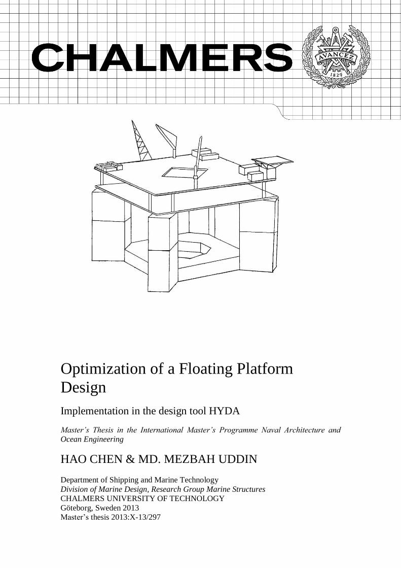
Optimization of a Floating Platform
Design
Implementation in the design tool HYDA
Master’s Thesis in the International Master’s Programme Naval Architecture and
Ocean Engineering
HAO CHEN & MD. MEZBAH UDDIN
Department of Shipping and Marine Technology
Division of Marine Design, Research Group Marine Structures
CHALMERS UNIVERSITY OF TECHNOLOGY
Göteborg, Sweden 2013
Master’s thesis 2013:X-13/297

MASTER’S THESIS IN THE INTERNATIONAL MASTER’S PROGRAMME IN
NAVAL ARCHITECTURE AND OCEAN ENGINEERING
Optimization of a Floating Platform DesignDesign
Implementation in the design tool HYDA
HAO CHEN & MD. MEZBAH UDDIN
Department of Shipping and Marine Technology
Division of Marine Design
Research Group Marine Structures
CHALMERS UNIVERSITY OF TECHNOLOGY
Göteborg, Sweden 2013
Optimization of a Floating Platform DesignDesign Implementation in the design tool HYDA
HAO CHEN & MD. MEZBAH UDDIN
© HAO CHEN & MD.MEZBAH UDDIN 2013
Master’s Thesis 2013:X-13/297
ISSN 1652-8557
Department of Shipping and Marine Technology
Division of Marine Design
Research Group Marine Structures
Chalmers University of Technology
SE-412 96 Göteborg
Sweden
Telephone: + 46 (0)31-772 1000
Chalmers Reproservice / Department of Shipping and Marine Technology
Göteborg, Sweden 2013

I
Optimization of a Floating Platform Design
Implementation in the design tool HYDA
Master’s Thesis in the International Master’s Programme in Naval Architecture and
Ocean Engineering
HAO CHEN & MD. MEZBAH UDDIN
Department of Shipping and Marine Technology
Division of Marine Design
Research Group Marine Structures
Chalmers University of Technology
ABSTRACT
The design tool HYDA is a FORTRAN program developed at GVA with the purpose
of aiding in the design and optimization of floating platforms. In this project a couple
of sub-routines that are considered to be of particular interest in HYDA are refined.
The considered sub-routines estimate mass budget, wind force, current force, mooring
stiffness and static offset. The estimated mass budget is interpolated from two
reference models; superstructure and area of facilities on deck are accounted for wind
force scaling. For mooring systems, the mean drift force is calculated and included in
the sub-routine responsible for calculating static offset and line tension. Moreover,
motion responses of three different platforms are evaluated and optimization of the
non-conventional unit is assessed using HYDA. The results before and after
optimization are listed and compared in this report. From the comparison it can be
concluded that the width of the platform after optimization is significantly reduced
while the eigenperiod increases. Both of the non-conventional units before and after
optimization give a good result in heave motion, which is considerably reduced
compared to a conventional unit.
Key words: floating platform, hydrodynamics, optimization,

II
CHALMERS, Shipping and Marine Technology, Master’s Thesis 2013:X-13/297 III
Contents
ABSTRACT I
CONTENTS III
PREFACE VII
NOTATIONS VIII
1 INTRODUCTION 1
1.1 Background 1
1.2 Objective 2
2 DESIGN TOOL HYDA 3
2.1 Existing design tool 3
2.2 New contributions to design tool 4
3 ENVIRONMENT CONDITIONS 6
3.1 Wind conditions 6
3.2 Current conditions 6
3.3 Wave conditions 6
4 RESPONSE TARGET 7
5 REFERENCE PLATFORM MODELS 9
5.1 Production unit 9
5.1.1 Geometrical description and panel model 9
5.1.2 Environmental condition 10
5.1.3 Computational result 10
5.2 Drilling unit 12
5.2.1 Geometrical description and panel model 12
5.2.2 Environmental condition 13
5.2.3 Computational result 13
5.3 Non-conventional unit 14
5.3.1 Geometrical description and panel model 14
5.3.2 Environmental condition 15
5.3.3 Computational result 15
6 INFLUENCE OF PANEL SIZE 17
7 MASS BUDGET SCALING 18
7.1 Existing mass budget scaling 18
7.2 New contributions to mass budget scaling 18

CHALMERS, Shipping and Marine Technology, Master’s Thesis 2013:X-13/297 IV
7.2.1 New created functions for mass budget 18
7.2.2 Modification of the relevant source code 19
7.2.3 Limitations 20
8 WIND-FORCE SCALING 21
8.1 Wind loads on offshore structures 21
8.2 Existing wind-force scaling 21
8.3 New contributions to wind-force scaling 22
8.3.1 New created function for wind-force scaling 22
8.3.2 Modification of relevant source code 23
8.3.3 Limitations 23
9 CURRENT FORCE CALCULATION 24
9.1 Current loads on offshore structures 24
9.2 Existing current force calculation 25
9.3 New contributions to current force calculation 26
9.3.1 Modification on current force calculation 26
9.3.2 Limitations 26
10 MOORING SYSTEMS 28
10.1 Introduction to mooring systems 28
10.2 Static analysis of mooring systems 28
10.2.1 Static analysis of a cable line 28
10.2.2 Analysis of spread mooring system 32
10.3 Existing subroutine for mooring system 33
10.3.1 Mooring stiffness calculation 33
10.3.2 Static offset calculation 34
10.4 Modification of the subroutine for mooring system 34
10.4.1 Modification of the subroutine for mooring stiffness 34
10.4.2 Modification of the subroutine for static offset 34
11 MEAN DRIFT FORCE IN OFFSET CALCULATION 35
11.1 Mean drift force on offshore structures 35
11.2 Calculation of mean drift force in HYDA 36
12 OPTIMIZATION OF NON-CONVENTIONAL UNIT 37
12.1 Optimization algorithm 37
12.2 Framework of the analysis 37
12.2.1 Analysis domain 37
12.2.2 Motion time scale 37
12.2.3 Coupling effects 37
12.3 Optimization of non-conventional unit 38
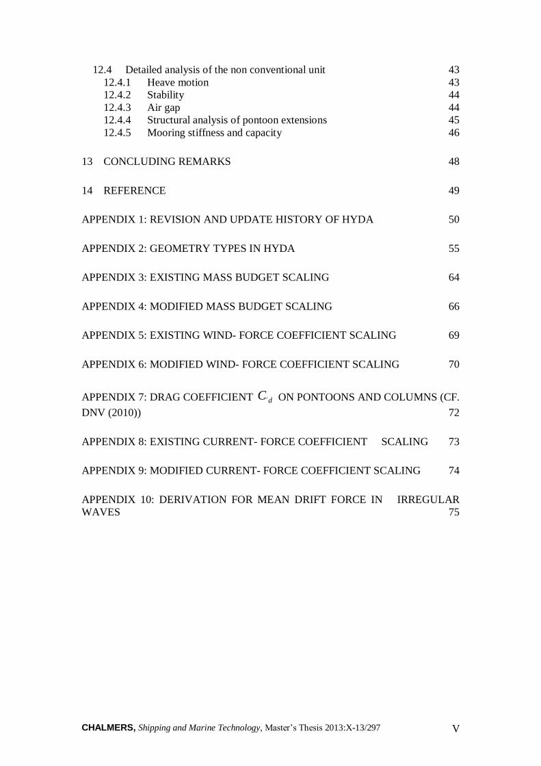
CHALMERS, Shipping and Marine Technology, Master’s Thesis 2013:X-13/297 V
12.4 Detailed analysis of the non conventional unit 43
12.4.1 Heave motion 43
12.4.2 Stability 44
12.4.3 Air gap 44
12.4.4 Structural analysis of pontoon extensions 45
12.4.5 Mooring stiffness and capacity 46
13 CONCLUDING REMARKS 48
14 REFERENCE 49
APPENDIX 1: REVISION AND UPDATE HISTORY OF HYDA 50
APPENDIX 2: GEOMETRY TYPES IN HYDA 55
APPENDIX 3: EXISTING MASS BUDGET SCALING 64
APPENDIX 4: MODIFIED MASS BUDGET SCALING 66
APPENDIX 5: EXISTING WIND- FORCE COEFFICIENT SCALING 69
APPENDIX 6: MODIFIED WIND- FORCE COEFFICIENT SCALING 70
APPENDIX 7: DRAG COEFFICIENT dC´ ON PONTOONS AND COLUMNS (CF.
DNV (2010)) 72
APPENDIX 8: EXISTING CURRENT- FORCE COEFFICIENT SCALING 73
APPENDIX 9: MODIFIED CURRENT- FORCE COEFFICIENT SCALING 74
APPENDIX 10: DERIVATION FOR MEAN DRIFT FORCE IN IRREGULAR
WAVES 75

CHALMERS, Shipping and Marine Technology, Master’s Thesis 2013:X-13/297 VI

CHALMERS, Shipping and Marine Technology, Master’s Thesis 2013:X-13/297 VII
Preface
This thesis is a part of the requirements for the master’s degree in Naval Architecture
and Ocean Engineering at Chalmers University of Technology, Göteborg, and has
been carried out at the Division of Marine Design, Department of Shipping and
Marine Technology, Chalmers University of Technology between January and June of
2013. We really appreciate many people who have given us a lot of help.
We would like to acknowledge and thank our supervisor Göran Johansson, Carl-Erik
Janson and Professor Jonas Ringsberg for sharing their knowledge and experience and
providing guidance to us. It has been impossible to implement the project without
their help.
Moreover, we would like to thank all the staff of the Hydrodynamic Department in
GVA.
Göteborg, June 2013
Hao Chen and Md. Mezbah Uddin
CHALMERS, Shipping and Marine Technology, Master’s Thesis 2013:X-13/297 VIII
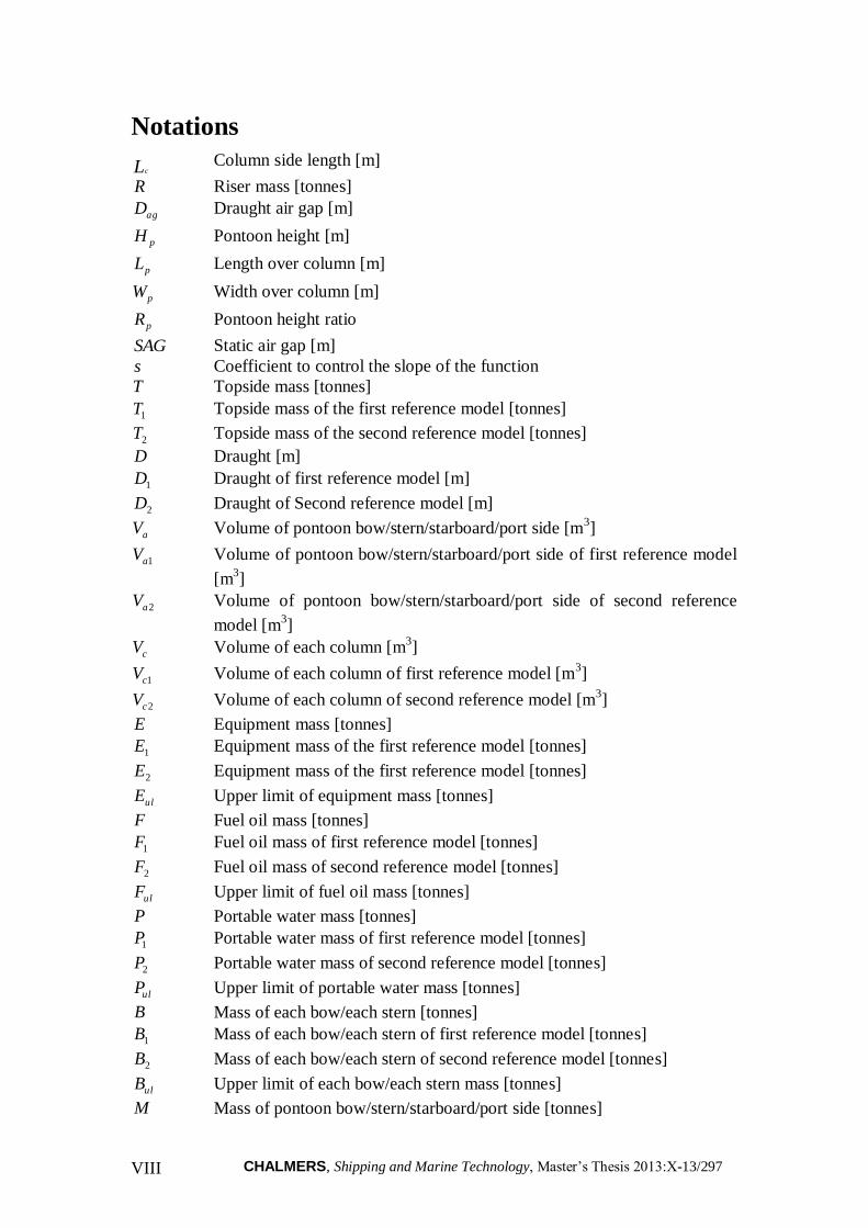
Notations
Lc Column side length [m]
R Riser mass [tonnes]
agD Draught air gap [m]
pH Pontoon height [m]
pL Length over column [m]
pW Width over column [m]
pR Pontoon height ratio
SAG Static air gap [m]
s Coefficient to control the slope of the function
T Topside mass [tonnes]
1T Topside mass of the first reference model [tonnes]
2T Topside mass of the second reference model [tonnes]
D Draught [m]
1D Draught of first reference model [m]
2D Draught of Second reference model [m]
aV Volume of pontoon bow/stern/starboard/port side [m3]
1aV Volume of pontoon bow/stern/starboard/port side of first reference model
[m3]
2aV Volume of pontoon bow/stern/starboard/port side of second reference
model [m3]
cV Volume of each column [m3]
1cV Volume of each column of first reference model [m3]
2cV Volume of each column of second reference model [m3]
E Equipment mass [tonnes]
1E Equipment mass of the first reference model [tonnes]
2E Equipment mass of the first reference model [tonnes]
ulE Upper limit of equipment mass [tonnes]
F Fuel oil mass [tonnes]
1F Fuel oil mass of first reference model [tonnes]
2F Fuel oil mass of second reference model [tonnes]
ulF Upper limit of fuel oil mass [tonnes]
P Portable water mass [tonnes]
1P Portable water mass of first reference model [tonnes]
2P Portable water mass of second reference model [tonnes]
ulP Upper limit of portable water mass [tonnes]
B Mass of each bow/each stern [tonnes]
1B Mass of each bow/each stern of first reference model [tonnes]
2B Mass of each bow/each stern of second reference model [tonnes]
ulB Upper limit of each bow/each stern mass [tonnes]
M Mass of pontoon bow/stern/starboard/port side [tonnes]
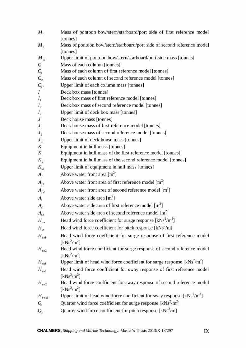
CHALMERS, Shipping and Marine Technology, Master’s Thesis 2013:X-13/297 IX
1M Mass of pontoon bow/stern/starboard/port side of first reference model
[tonnes]
2M Mass of pontoon bow/stern/starboard/port side of second reference model
[tonnes]
ulM Upper limit of pontoon bow/stern/starboard/port side mass [tonnes]
C Mass of each column [tonnes]
1C Mass of each column of first reference model [tonnes]
2C Mass of each column of second reference model [tonnes]
ulC Upper limit of each column mass [tonnes]
I Deck box mass [tonnes]
1I Deck box mass of first reference model [tonnes]
2I Deck box mass of second reference model [tonnes]
ulI Upper limit of deck box mass [tonnes]
J Deck house mass [tonnes]
1J Deck house mass of first reference model [tonnes]
2J Deck house mass of second reference model [tonnes]
ulJ Upper limit of deck house mass [tonnes]
K Equipment in hull mass [tonnes]
1K Equipment in hull mass of the first reference model [tonnes]
2K Equipment in hull mass of the second reference model [tonnes]
ulK Upper limit of equipment in hull mass [tonnes]
fA Above water front area [m2]
1fA Above water front area of first reference model [m2]
2fA Above water front area of second reference model [m2]
sA Above water side area [m2]
1sA Above water side area of first reference model [m2]
2sA Above water side area of second reference model [m2]
suH Head wind force coefficient for surge response [kNs2/m
2]
pH Head wind force coefficient for pitch response [kNs2/m]
1suH Head wind force coefficient for surge response of first reference model
[kNs2/m
2]
2suH Head wind force coefficient for surge response of second reference model
[kNs2/m
2]
sulH Upper limit of head wind force coefficient for surge response [kNs2/m
2]
1swH Head wind force coefficient for sway response of first reference model
[kNs2/m
2]
2swH Head wind force coefficient for sway response of second reference model
[kNs2/m
2]
swulH Upper limit of head wind force coefficient for sway response [kNs2/m
2]
sQ Quarter wind force coefficient for surge response [kNs2/m
2]
pQ Quarter wind force coefficient for pitch response [kNs2/m]
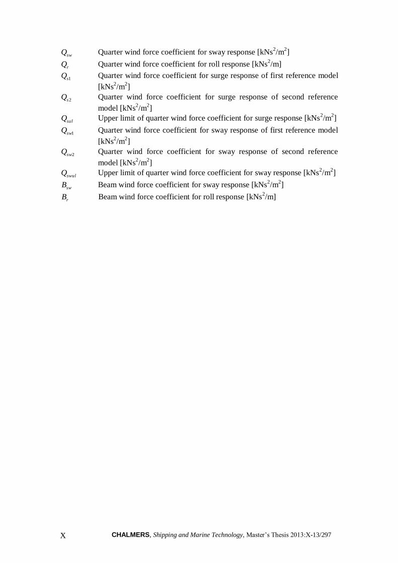
CHALMERS, Shipping and Marine Technology, Master’s Thesis 2013:X-13/297 X
swQ Quarter wind force coefficient for sway response [kNs2/m
2]
rQ Quarter wind force coefficient for roll response [kNs2/m]
1sQ Quarter wind force coefficient for surge response of first reference model
[kNs2/m
2]
2sQ Quarter wind force coefficient for surge response of second reference
model [kNs2/m
2]
sulQ Upper limit of quarter wind force coefficient for surge response [kNs2/m
2]
1swQ Quarter wind force coefficient for sway response of first reference model
[kNs2/m
2]
2swQ Quarter wind force coefficient for sway response of second reference
model [kNs2/m
2]
swulQ Upper limit of quarter wind force coefficient for sway response [kNs2/m
2]
swB Beam wind force coefficient for sway response [kNs2/m
2]
rB Beam wind force coefficient for roll response [kNs2/m]
CHALMERS, Shipping and Marine Technology, Master’s Thesis 2013:X-13/297 1
1 Introduction
1.1 Background
Knowledge about the environmental load and motion of offshore structures is of
importance both in design and operation. The induced motion response can have a
significant impact on offshore structures. Heave motion is a limiting factor for drilling
operations since the vertical motion of risers has to be compensated and there are
limits to how much the motion can be compensated. Similarly, on a production unit
the heave motion impacts on the riser design. Rolling, pitching and accelerations may
represent limiting factors for the operation of process equipment on board.
Generally speaking, offshore platforms can be divided into fixed structures and
floating platforms. Jack-up and gravity-based structures are typical fixed offshore
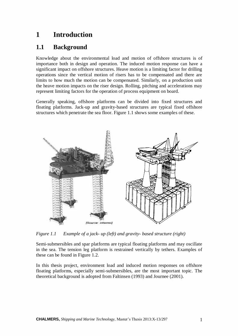
structures which penetrate the sea floor. Figure 1.1 shows some examples of these.
Figure 1.1 Example of a jack- up (left) and gravity- based structure (right)
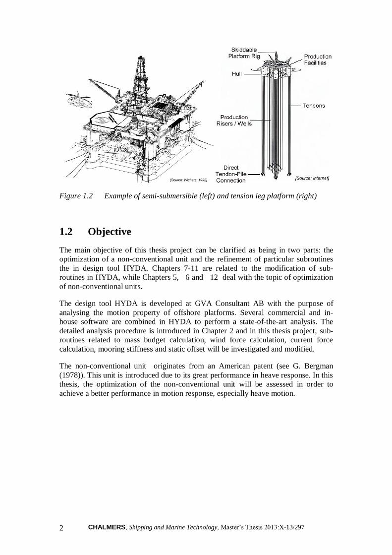
Semi-submersibles and spar platforms are typical floating platforms and may oscillate
in the sea. The tension leg platform is restrained vertically by tethers. Examples of
these can be found in Figure 1.2.
In this thesis project, environment load and induced motion responses on offshore
floating platforms, especially semi-submersibles, are the most important topic. The
theoretical background is adopted from Faltinsen (1993) and Journee (2001).
CHALMERS, Shipping and Marine Technology, Master’s Thesis 2013:X-13/297 2
Figure 1.2 Example of semi-submersible (left) and tension leg platform (right)
1.2 Objective
The main objective of this thesis project can be clarified as being in two parts: the
optimization of a non-conventional unit and the refinement of particular subroutines
the in design tool HYDA. Chapters 7-11 are related to the modification of sub-
routines in HYDA, while Chapters 5, 6 and 12 deal with the topic of optimization
of non-conventional units.
The design tool HYDA is developed at GVA Consultant AB with the purpose of
analysing the motion property of offshore platforms. Several commercial and in-
house software are combined in HYDA to perform a state-of-the-art analysis. The
detailed analysis procedure is introduced in Chapter 2 and in this thesis project, sub-
routines related to mass budget calculation, wind force calculation, current force
calculation, mooring stiffness and static offset will be investigated and modified.
The non-conventional unit originates from an American patent (see G. Bergman
(1978)). This unit is introduced due to its great performance in heave response. In this
thesis, the optimization of the non-conventional unit will be assessed in order to
achieve a better performance in motion response, especially heave motion.
CHALMERS, Shipping and Marine Technology, Master’s Thesis 2013:X-13/297 3
2 The Design Tool HYDA
2.1 Existing design tool
HYDA is a FORTRAN program developed at GVA with the purpose of aiding in the
design of floating platforms. Depending on the input specified by the users, different
sub-routines are called by HYDA either in a sequence or in an iterative fashion.
The input data is stored in the input file HYDA.INP, which will be called by HYDA
when the program starts to run. The input data is divided into four categories:
1. Primary input, which includes environmental conditions and predefined
topside and riser mass.
2. Secondary input, which includes geometric dimensions of the platform.
3. Tertiary input, which includes mesh size of the panel model, optimization
option, etc.
4. Target values for the optimization process, which include target heel, target
heave, target ballast, etc.
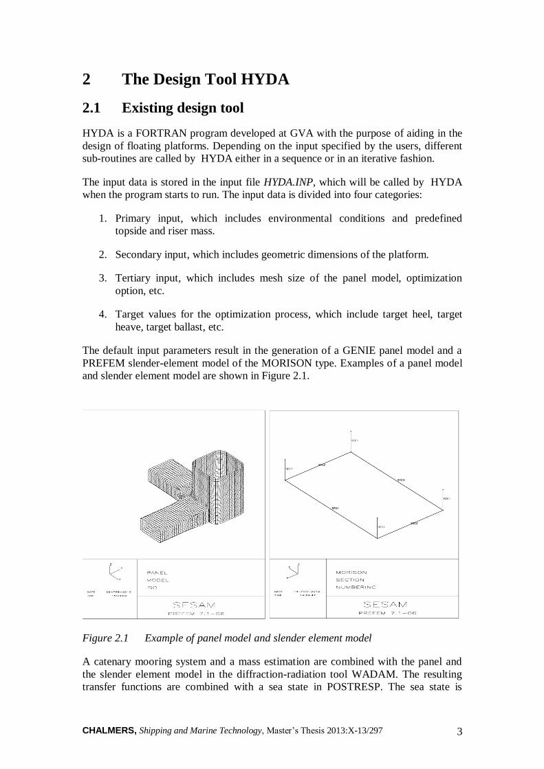
The default input parameters result in the generation of a GENIE panel model and a
PREFEM slender-element model of the MORISON type. Examples of a panel model
and slender element model are shown in Figure 2.1.
Figure 2.1 Example of panel model and slender element model
A catenary mooring system and a mass estimation are combined with the panel and
the slender element model in the diffraction-radiation tool WADAM. The resulting
transfer functions are combined with a sea state in POSTRESP. The sea state is
CHALMERS, Shipping and Marine Technology, Master’s Thesis 2013:X-13/297 4
represented by the PIERSON-MOSKOWITZ spectrum in POSTRESP. The calculated
motion characteristics include:
1. Eigenperiods and associated eigenvectors which are calculated in WADAM.
2. Static offsets calculated in the HYDA subroutine CATMOOR from the wind
and current force coefficients combined with the mooring stiffness.
3. Stability at operation and in quay conditions.
4. Response amplitude operators for motions of six degree of freedoms due to
waves propagating towards the bow, quartering sea and beam sea.
5. Calculated motion response and most probable minimum air-gap.
The key results of the calculation are combined with their respective target values to
form an object function, which is the criterion for the program to assess the
performance of the optimization. If the optimization option is activated, then HYDA
uses the input parameter values as a starting guess and strives to minimize the object
function via minimization algorithms. A SIMPLEX type of minimization algorithm is
adopted here.
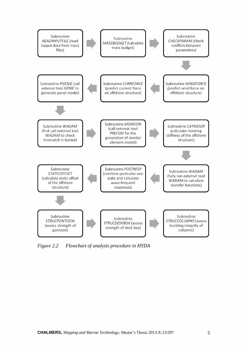
The analysis procedure mentioned above is summarized as a flow chart which is
shown in Figure 2.2.
2.2 New contributions to the design tool
In this project, new contributions to the design tool HYDA are the modification of
several sub-routines in the tool and studies of a non-conventional platform.
The modified subroutines include mass budget scaling, wind-force scaling, current-
force scaling and mooring systems. The estimated mass budget is interpolated from
two reference models. For wind-force resistance, data of one reference model from a
wind tunnel test are considered in the same way as for mass budget. For mooring
systems, mean drift forces are included in the subroutine for calculating static offset
and line tension.
Motion responses of three different platforms are analysed using HYDA in this
project, and special attention is paid to a special non-conventional unit. The design of
the non-conventional unit is optimized in HYDA via the SIMPLEX algorithm in order
to minimize the object function and the motion response.
CHALMERS, Shipping and Marine Technology, Master’s Thesis 2013:X-13/297 5
Figure 2.2 Flowchart of analysis procedure in HYDA
CHALMERS, Shipping and Marine Technology, Master’s Thesis 2013:X-13/297 6
3 Environmental Conditions
Environmental conditions cover natural phenomena, which may contribute to
structural damage, operation disturbances or navigation failures. The most important
phenomena for marine structures are wind, waves and current.
3.1 Wind conditions
Wind speed varies with time and height above the sea surface. For theses reasons, the
averaging time for wind speeds and the reference height must be specified. A
commonly used reference height is 10H m. commonly used averaging time are 1
minute, 10 minutes and 1 hour. In this project, the average wind velocity over 1 hour
at a height of 10 metres is adopted.
3.2 Current conditions
The current velocity vector varies with water depth. Close to the water surface the
current velocity profile is stretched or compressed due to surface waves. However, in
this project, the current is considered as a steady flow field and constant over depth.
3.3 Wave conditions
Short-term stationary irregular sea states may be described by a wave spectrum
formulated by a set of parameters such as the significant wave height and peak period.
In this project the PIERSON-MOSKOWITZ (PM) spectrum is adopted, which is given
by:
4
542
4
5exp
16
5)(
p
psPM HS
(3.1)
where is the wave frequency, sH is the significant wave height, pT is the peak
period and pp T/2 is the angular spectral peak frequency,
CHALMERS, Shipping and Marine Technology, Master’s Thesis 2013:X-13/297 7
4 Response Target
In order to distinguish a good design from a less good design we make use of typical
design targets. Design targets are typically determined by customer requirements,
equipment limitations and regulations.
In this chapter, the design target values of a non-conventional unit are introduced and
they will be used in the optimization of a non-conventional unit in Chapter 12. The
considered responses include:
Heave amplitude, which is a critical criterion for the platform.
Metacentric height, which represents the initial stability of the platform.
Acceleration, which the human body is very sensitive to.
Pontoon stress level, which indicates the strength of the pontoon.
Mass of platform, which is related to the cost of the platform.
Air gap, which is the distance between the wave crest and main deck of the
platform.
Static offset, which is the static displacement in the horizontal plane under
wave, current and wind-force.
Heel amplitude, which represents the static inclination under wind and current.
Eigenperiod associated with heave motion, which indicates the probability that
resonance happens.
The geometric dimension includes length, width or draught of platforms. Sometimes
there are geometrical limitations in terms of dimension of a dry dock and water depth
of the operation area. The length or width of floating platform is restricted due to
width or length of dry dock. The draught of the platform could also be a restriction
due to water depth of the sea, which often happens for a drilling unit since it is towed
between different locations.
The target values of these responses are shown in Table 4.1. The calculated results are
combined with their target values to form an objective function f defined as:
2
arg
arg
ett
i
ett
ii
calculated
i
i
iX
XbXaf (4.1)
where:
calculated
iX is the calculated response.
ett
iX arg is the target response.

CHALMERS, Shipping and Marine Technology, Master’s Thesis 2013:X-13/297 8
ia and ib are the weighting factors, which is defined by users according to the
importance of the response in this optimization process. The default values are shown
in Table 3.1. When the calculated result for a response fulfils the target values, ia
will automatically change to zero, and thus no values will be added to the objective
function regarding this response.
The object function can partially reflect the difference between target values and
calculation results. If the result of the object function is low then the design model
may be close to target requirement. The case with the minimum value of the object
function, which offers good results in all the considered responses, can be chosen as
the optimized design.
Table 4.1 Design target values for a non-conventional unit and default value of
weighting factors
Considered response and geometrical
limits
Target value ia ib
Heave amplitude ≤2.0 m 2 0
Metacentric height ≥2 m 2 1
Acceleration ≤0.15g 1 1
Pontoon stress level ≤100 MPa 1 1
Displaced mass ≤10000 tonnes 2 1
Air gap ≥1.0 m 2 1
Heel amplitude ≤5.5˚ 2 0
Offset amplitude ≤7% of water depth 1 0
Eigen period associated with heave
motion
≥22 s --- ---
Draught 30 m 2 0
Width 80 m 2 0
CHALMERS, Shipping and Marine Technology, Master’s Thesis 2013:X-13/297 9
5 Reference Platform Models
In this Chapter, three different types of reference models are introduced and evaluated
in HYDA. The geometric characteristic for each reference model is illustrated in
Appendix 2, and here the typical computational results are shown and analysed.
5.1 Production unit
5.1.1 Geometric description and panel model
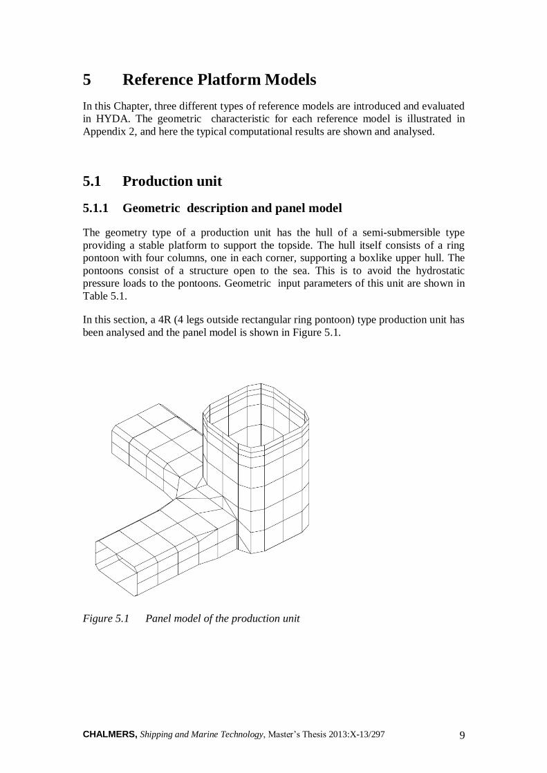
The geometry type of a production unit has the hull of a semi-submersible type
providing a stable platform to support the topside. The hull itself consists of a ring
pontoon with four columns, one in each corner, supporting a boxlike upper hull. The
pontoons consist of a structure open to the sea. This is to avoid the hydrostatic
pressure loads to the pontoons. Geometric input parameters of this unit are shown in
Table 5.1.
In this section, a 4R (4 legs outside rectangular ring pontoon) type production unit has
been analysed and the panel model is shown in Figure 5.1.
Figure 5.1 Panel model of the production unit
CHALMERS, Shipping and Marine Technology, Master’s Thesis 2013:X-13/297 10
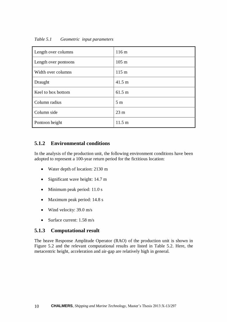
Table 5.1 Geometric input parameters
Length over columns 116 m
Length over pontoons 105 m
Width over columns 115 m
Draught 41.5 m
Keel to box bottom 61.5 m
Column radius 5 m
Column side 23 m
Pontoon height 11.5 m
5.1.2 Environmental conditions
In the analysis of the production unit, the following environment conditions have been
adopted to represent a 100-year return period for the fictitious location:
Water depth of location: 2130 m
Significant wave height: 14.7 m
Minimum peak period: 11.0 s
Maximum peak period: 14.8 s
Wind velocity: 39.0 m/s
Surface current: 1.58 m/s
5.1.3 Computational result
The heave Response Amplitude Operator (RAO) of the production unit is shown in
Figure 5.2 and the relevant computational results are listed in Table 5.2. Here, the
metacentric height, acceleration and air-gap are relatively high in general.

CHALMERS, Shipping and Marine Technology, Master’s Thesis 2013:X-13/297 11
Figure 5.2 Heave RAO of Production unit
Table 5.2 Calculation results for the production unit
Considered response Results from analysis model
Heave amplitude 3.5 m
Metacentric height 8.9 m
Acceleration 0.7g
Stress level 256 MPa
Displaced mass 143000 tonnes
Air gap 12.1m
Heel amplitude 6.4˚
Offset amplitude 6.9% of water depth
Eigen period associated with
heave motion
22.7 s
CHALMERS, Shipping and Marine Technology, Master’s Thesis 2013:X-13/297 12
5.2 Drilling unit
5.2.1 Geometrical description and panel model
An offshore drilling unit can move to different locations for a drilling operation. Here,
a drilling unit (D4) is analysed using HYDA. A panel model of this unit is shown in
Figure 5.3. Geometric input parameters of this unit are shown in Table 5.3.
Figure 5.3 Panel model of the drilling unit
Table 5.3 Geometric input parameters
Length over pontoons 89.7 m
Pontoon height 9.1 m
Width over columns 70.7 m
Draught 25 m
Keel to box bottom 35.9 m
Column radius 5 m
Column side 13.7 m
Width of wing 10 m
Wing height 3 m

CHALMERS, Shipping and Marine Technology, Master’s Thesis 2013:X-13/297 13
5.2.2 Environmental conditions
In the analysis of the drilling unit, the following environmental conditions have been
adopted to represent a 100-year return period for the fictitious location:
Water depth of location: 500 m
Significant wave height: 13.4 m
Minimum peak period: 11.5 s
Maximum peak period: 15.0 s
Wind velocity: 26.7 m/s
Surface current: 0.6 m/s
5.2.3 Computational result
The heave Response Amplitude Operator (RAO) of the drilling unit is shown in
Figure 5.4 and the selected computational results are listed in Table 5.4. Here, the
heave amplitude and acceleration are rather high, which may affect the drilling
operation. Also an unexpected negative air-gap occurred, which may result in a
wave-in-deck force and structural damage may occur.
Figure 5.4 Heave RAO of drilling unit

CHALMERS, Shipping and Marine Technology, Master’s Thesis 2013:X-13/297 14
Table 5.4 Calculation results for the drilling unit
Considered response Results from analysis model
Heave amplitude 5.1m
Metacentric height 1.0 m
Acceleration 1.1g
Stress level 75 MPa
Displaced mass 39000 tonnes
Air gap -2.1 m
Heel amplitude 5.4˚
Offset amplitude 6.4% of water depth
Eigen period associated with
heave motion
23.6 s
5.3 The non-conventional unit
5.3.1 Geometric description and panel model
This section is devoted to the study of a non-conventional unit. The non-conventional
semi-submersible structure includes a platform supported by columns and the
pontoons disposed inboard between the columns as well as longitudinally outboard
extension of the columns. A panel model of the considered non-conventional unit
(U2) is shown in Figure 5.5. Geometric input parameters of this unit are shown in
Table 5.5.
Figure 5.5 Panel model of the non-conventional unit

CHALMERS, Shipping and Marine Technology, Master’s Thesis 2013:X-13/297 15
Table 5.5 Geometrical input parameters
Length over pontoons 90 m
Pontoon height 5 m
Pontoon width 5 m
Draught 30 m
Keel to box bottom 40 m
Front height 15 m
Front width 15 m
Column side 16 m
Width of wing 5 m
5.3.2 Environmental conditions
In the analysis of the non-conventional unit in Chapters 5 and 12, the following data
is adopted to represent a 100-year return period for the fictitious location:
Water depth of location: 500 m
Significant wave height: 14.0 m
Minimum peak period: 11.0 s
Maximum peak period: 14.0 s
Wind velocity: 26.67 m/s
Surface current: 0.63 m/s
5.3.3 Computational result
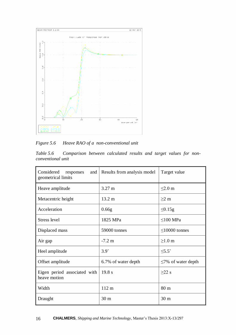
The heave RAO of the non-conventional unit is illustrated in Figure 5.6 and the
comparison between calculated results and the target values for non-conventional unit
is listed in Table 5.6. From Figure 5.6 it can be seen that this type of platform has a
good performance in terms of heave motion. But the main problems are the large
negative air-gap and also the large width and low eigenperiod.
CHALMERS, Shipping and Marine Technology, Master’s Thesis 2013:X-13/297 16
Figure 5.6 Heave RAO of a non-conventional unit
Table 5.6 Comparison between calculated results and target values for non-
conventional unit
Considered responses and
geometrical limits
Results from analysis model Target value
Heave amplitude 3.27 m ≤2.0 m
Metacentric height 13.2 m ≥2 m
Acceleration 0.66g ≤0.15g
Stress level 1825 MPa ≤100 MPa
Displaced mass 59000 tonnes ≤10000 tonnes
Air gap -7.2 m ≥1.0 m
Heel amplitude 3.9˚ ≤5.5˚
Offset amplitude 6.7% of water depth ≤7% of water depth
Eigen period associated with
heave motion
19.8 s ≥22 s
Width 112 m 80 m
Draught 30 m 30 m
CHALMERS, Shipping and Marine Technology, Master’s Thesis 2013:X-13/297 17
6 The Influence of Panel Size
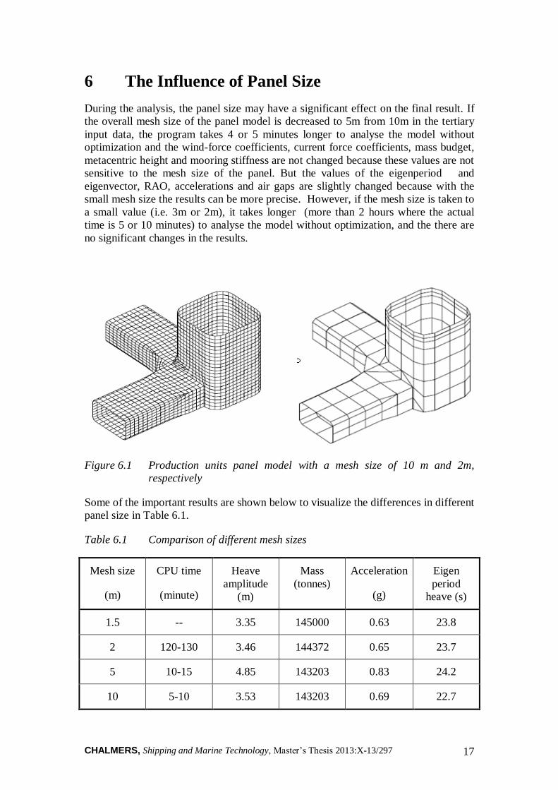
During the analysis, the panel size may have a significant effect on the final result. If
the overall mesh size of the panel model is decreased to 5m from 10m in the tertiary
input data, the program takes 4 or 5 minutes longer to analyse the model without
optimization and the wind-force coefficients, current force coefficients, mass budget,
metacentric height and mooring stiffness are not changed because these values are not
sensitive to the mesh size of the panel. But the values of the eigenperiod and
eigenvector, RAO, accelerations and air gaps are slightly changed because with the
small mesh size the results can be more precise. However, if the mesh size is taken to
a small value (i.e. 3m or 2m), it takes longer (more than 2 hours where the actual
time is 5 or 10 minutes) to analyse the model without optimization, and the there are
no significant changes in the results.
Figure 6.1 Production units panel model with a mesh size of 10 m and 2m,
respectively
Some of the important results are shown below to visualize the differences in different
panel size in Table 6.1.
Table 6.1 Comparison of different mesh sizes
Mesh size
(m)
CPU time
(minute)
Heave
amplitude
(m)
Mass
(tonnes)
Acceleration
(g)
Eigen
period
heave (s)
1.5 -- 3.35 145000 0.63 23.8
2 120-130 3.46 144372 0.65 23.7
5 10-15 4.85 143203 0.83 24.2
10 5-10 3.53 143203 0.69 22.7
CHALMERS, Shipping and Marine Technology, Master’s Thesis 2013:X-13/297 18
7 Mass Budget Scaling
The mass, the centre of the gravity and the radii of gyration with respect to the still
water line are estimated in the subroutine MASSBUDGET, which is based on a
typical minimum equipment list and geometric dimensions.
The mass of some items of the floating platform is regarded as primary input data in
the program, and for remaining items the mass will be generated via the subroutine
MASSBUDGET. It is necessary to use some scaling factors and reference values to
generate the mass of the remaining items in the equipment list subroutine of the
program. These scaling factors and the reference values are based on experience and
existing platform design.
7.1 Existing mass budget scaling
In the initial mass budget, only one model is referred to as a reference model and it is
assumed that there is a linear relationship between the reference model and the
studied model. Items of the floating platform are listed in Appendix 3, which
illustrates how their mass is scaled in the subroutine equipmentlist1. Here, the scaling
of the equipment mass is illustrated as an example and the scaling formula is given as
follows:
1
1T
TEE (7.1)
where E is the equipment mass of the studied model, 1E is the equipment mass of the
reference model. T is the topside mass of the studied model, 1T is the topside mass of
the reference model.
The existing mass budget for each item is tabulated in Appendix 3.
7.2 New contributions to mass budget scaling
It is not always appropriate to estimate the mass of different items only based on one
reference model, since it is very probable that there is a significant difference
between the reference model and the estimated model. So it is favourable to make a
further investigation into improving the accuracy of mass scaling.
7.2.1 New created functions for mass budget
One possible solution for the mass budget is to establish the estimation function based
on two reference models. The piecewise function is adopted and in order to set an
upper limit to make the estimation more reasonable, the arctan function is adopted.
The piecewise function is continuous from zero to infinity and the result of the
prediction is dependent on the reference models.
CHALMERS, Shipping and Marine Technology, Master’s Thesis 2013:X-13/297 19
The updated equipment mass is scaled as follows:
If 1TT :
TT
EE
0
0
1
1 (7.2)
If 2TT :
2
2
2
1arctan/2 E
ssT
TEEE ul
(7.3)
If 21 TTT :
11
12
12 ETTTT
EEE
(7.4)
where ulE is the upper limit of the equipment mass for the studied model, 2E is the
equipment mass of second reference model. 2T is the topside mass of the second
reference model, s is the factor for controlling the slope of the function.
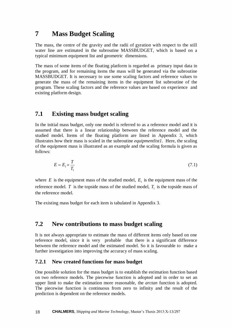
Figure 7.1 shows the predicted equipment mass versus the different given topside
mass. The updated mass budget for different items is listed in Appendix 4.
Figure 7.1 The predicted equipment mass vs. the given topside mass
7.2.2 Modification of the relevant source code
Based on the updated mass budget functions, the source code of subroutine
equipmentlist1 is updated. The reference models can be predefined or defined by the
users. There will be a new integer variable imass in the program to control the option.
If 1imass , the two reference models will be defined by users. Or 0imass , in
which case the predefined reference models will be used. The reason for setting this
variable is that if the user has better reference models, which are closed to the
CHALMERS, Shipping and Marine Technology, Master’s Thesis 2013:X-13/297 20
designed one, they should be adapted since models with similar geometry and
dimension will definitely give a better prediction of mass budget.
7.2.3 Limitations
The updated subroutine for mass budget scaling has some limitations and they will be
discussed in this section.
1. In the input file of the reference models, the order of the row cannot be
changed. This is mainly due to the fact that the program reads the input data
and assigns the value to the variables in a fixed way. If the order of the input
data is changed, the variables will be assigned the wrong values.
2. The name of the input data should not be changed. The names of the input data
for reference models are ref_model1.inp and ref_model2.inp. They cannot be
substituted with any other names, since the source code only opens the files
with these two names. If they do not exist, the program will be stopped.
3. The data of these two reference models should be reliable enough and similar
to the designed model. The accuracy of the prediction is to a large extent
dependent on the reference models.

CHALMERS, Shipping and Marine Technology, Master’s Thesis 2013:X-13/297 21
8 Wind Force Scaling
8.1 Wind loads on offshore structures
Wind-induced loads are in general time-dependent loads due to fluctuations in wind
velocity. The response of a structure due to wind loading can be partitioned into a
static and a dynamic contribution. Only the static response is accounted for here.
The wind pressure can be described by the following relationship (cf. DNV (2010)):
2
,2
1zTaUq (8.1)
where q is the wind pressure, a is mass density of air which is to be taken as 1.2
kg/m 3 . Moreover, 2
, zTU is the wind velocity averaged over a time T at a height
z metres above the mean water level.
The wind force wF on a structure member is formulated as:
CqSFw (8.2)
where C is the shape coefficient and q is the wind pressure as defined in equation
(8.2) and S is the projected area of the member normal to the direction of the force.
In this project, the projected area exposed to wind is not a previously known variable.
The adopted wind force coefficients CSk aw 2/1 are based on similar projects
scaled with respect to geometric dimensions (e.g. projected area S) in the subroutine
WINDFORCE.
8.2 Existing wind-force scaling
Similar to mass budget scaling, wind-force coefficients for different motions in
different directions are also scaled, based on some scaling factors and reference
values. These scaling factors and reference values are also taken based on existing
floating platforms. In the initial wind-force resistance scaling, surge force is scaled
with the multiplication of width and static air-gap, which can be roughly
approximated as an exposed area of the platform and only one reference model is
referred to. Sway force, pitch moment and roll moment are calculated based on the
surge force.
Here, the wind-force coefficient in a head direction for the surge response of the
studied model is illustrated as an example:
)/(58.4 11 SAGWSAGWF ppw (8.3)
CHALMERS, Shipping and Marine Technology, Master’s Thesis 2013:X-13/297 22
Where SAG is the static air-gap of the studied model, pW is the width over column of
the studied model, 1pW is the width over column of the reference model and 1SAG is
the static air-gap of the reference model.
The wind-force coefficients for different motions in each direction are tabulated in
Appendix 5.
8.3 New contributions to wind-force scaling
8.3.1 New created function for wind-force scaling
Factors which have influence on wind-force resistance are the wind area of a derrick,
topside module, deck box and column side along with their shape. These factors
should be accounted for in an updated subroutine.
Surge and sway force are proportional to the front and side area of the platform,
respectively. Piecewise functions are established based for interpolation between two
reference models. The pitch and roll moment can be regarded as a surge and sway
force times their levers. The lever can be approximated as the multiplication of static
air-gap and a scaling factor. This scaling factor is motivated from trends in
experimental wind tunnel data. The detailed formula can be referred to in Appendix 6.
The updated wind-force coefficient in a head direction for surge response is estimated
via the following formulas:
If 1ff AA :
f
f
ww A
A
FF
0
0
1
1 (8.4)
If 1ff AA :
2
2
2
1arctan/2 w
f
f
wwulw FssA
AFFF
(8.5)
If 21 fff AAA :
11
12
12
wff
ff
ww
w FAAAA
FFF
(8.6)
where fA , 1fA 2fA are the front areas of the studied model - the first and second
reference model above water. wF , 1wF 2wF are the wind-force coefficients of the
studied model - the first and second reference model. s is the factor for controlling
the slope of the function. wulF is the upper limit for the wind-force coefficient.

CHALMERS, Shipping and Marine Technology, Master’s Thesis 2013:X-13/297 23
8.3.2 Modification of the relevant source code
Similar manners are adopted in the subroutine for wind resistance scaling. The user
will determine if user-defined reference models or predefined reference models will
be adopted by defining the value of variable imass . The new created functions have
been introduced in the program. At the same time in the input file, three new items
have been added, namely the the exposed area of the derrick, the topside module and
the deck box height. They will be recognized by the program through the subroutine
readinputfile.
8.3.3 Limitations
1. The true lever for pitch and roll moments are approximated as a multiplication
of the scaling factor and static air-gap of the floating platform. Thus, it is not
always accurate for different kinds of platforms.
2. The factor is predefined in the program and therefore fixed for all types of
platforms. But the value of the factor is derived from regular semi-
submersibles so there will be errors for other types of platforms.
3. For user-defined reference models, detailed data from the reference model are
required, such as the derrick area, the topside module area, etc. Also, data for
these two reference models should be reliable since it will determine the
accuracy of the wind resistance scaling being to a large extent dependent on
the reference models.
CHALMERS, Shipping and Marine Technology, Master’s Thesis 2013:X-13/297 24
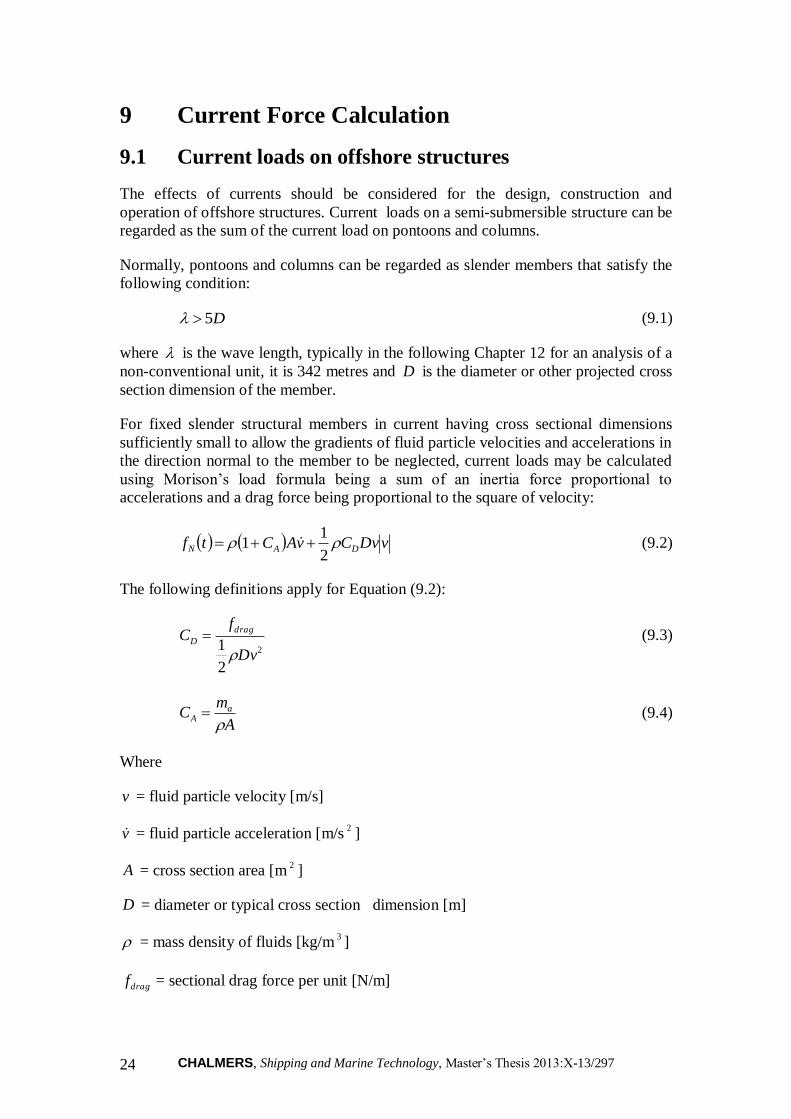
9 Current Force Calculation
9.1 Current loads on offshore structures
The effects of currents should be considered for the design, construction and
operation of offshore structures. Current loads on a semi-submersible structure can be
regarded as the sum of the current load on pontoons and columns.
Normally, pontoons and columns can be regarded as slender members that satisfy the
following condition:
D5 (9.1)
where is the wave length, typically in the following Chapter 12 for an analysis of a
non-conventional unit, it is 342 metres and D is the diameter or other projected cross
section dimension of the member.
For fixed slender structural members in current having cross sectional dimensions
sufficiently small to allow the gradients of fluid particle velocities and accelerations in
the direction normal to the member to be neglected, current loads may be calculated
using Morison’s load formula being a sum of an inertia force proportional to
accelerations and a drag force being proportional to the square of velocity:
vDvCvACtf DAN 2
11 (9.2)
The following definitions apply for Equation (9.2):
2
2
1Dv
fC
drag
D
(9.3)
A
mC a
A
(9.4)
Where
v = fluid particle velocity [m/s]
v = fluid particle acceleration [m/s2
]
A = cross section area [m2
]
D = diameter or typical cross section dimension [m]
= mass density of fluids [kg/m3]
dragf = sectional drag force per unit [N/m]
CHALMERS, Shipping and Marine Technology, Master’s Thesis 2013:X-13/297 25
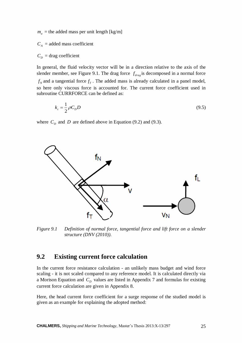
am = the added mass per unit length [kg/m]
AC = added mass coefficient
DC = drag coefficient
In general, the fluid velocity vector will be in a direction relative to the axis of the
slender member, see Figure 9.1. The drag force dragf is decomposed in a normal force
Nf and a tangential force Tf . The added mass is already calculated in a panel model,
so here only viscous force is accounted for. The current force coefficient used in
subroutine CURRFORCE can be defined as:
DCk Dc 2
1 (9.5)
where DC and D are defined above in Equation (9.2) and (9.3).
Figure 9.1 Definition of normal force, tangential force and lift force on a slender
structure (DNV (2010)).
9.2 Existing current force calculation
In the current force resistance calculation - an unlikely mass budget and wind force
scaling - it is not scaled compared to any reference model. It is calculated directly via
a Morison Equation and DC values are listed in Appendix 7 and formulas for existing
current force calculation are given in Appendix 8.
Here, the head current force coefficient for a surge response of the studied model is
given as an example for explaining the adopted method:

CHALMERS, Shipping and Marine Technology, Master’s Thesis 2013:X-13/297 26
2/)24( pc WsponDscolF (9.6)
The following definitions apply in Equation (9.6):
cdcol LCscol2
(9.7)
pdpon HCspon2
(9.8)
where D is the draught of the column, pW is the width over columns, dcolC is the drag
coefficient for columns, dponC is the drag coefficient for pontoons, cL is the column
side length and pH is the pontoon height.
9.3 New contributions to current force calculation
9.3.1 Modification on current force calculation
A Morison equation gives a good result in the estimation of the viscous effect on
pontoons and columns. In the modified subroutine, surge force and pitch moment are
kept unchanged and a small modification has been made for the sway and roll
response.
For example, the current force coefficient in the quarter direction for a sway response
of the studied model is as follows:
4.2/)24( ppc RLsponDscolF (9.9)
where pL is the length over column, pR is the pontoon height ratio. For a drilling unit
with 4 legs and a non-conventional unit with 4 legs and box appendices, pR is defined
as the ratio of the pontoon height and wing height. For other types of semi-
submersibles, it is equal to 1.
The detailed formula for the current force modification can be referred to in Appendix
9.
9.3.2 Limitations
For the calculation of current force coefficients, there are a couple of limitations that
should be observed:
1. Wake interaction is not accounted for in the calculation of current force. For a
regular semi-submersible platform, there should be four columns, two of
which are in the upstream of the incident flow and another two are in the
downstream. The force on the cylinder downstream of another cylinder
upstream is influenced by the wake generated by the upstream cylinder. The

CHALMERS, Shipping and Marine Technology, Master’s Thesis 2013:X-13/297 27
main effects on the mean forces on the downstream cylinder is the reduced
mean drag force due to shielding effects and the non-zero lift force due to
velocity gradients in the wake field. But in subroutine CURRFORCE, this
effect is not included. However, regarding drag force, it is a conservative
estimate if taken out of the vortex shielding.
2. The Current load is considered to be separated from the wave load. WADAM
has a limitation that can only be solved by a linear equation , so coupled
effects of waves and currents are not accounted for in WADAM.

CHALMERS, Shipping and Marine Technology, Master’s Thesis 2013:X-13/297 28
10 Mooring Systems
10.1 Introduction to mooring systems
The precise positioning and long-term motion control of offshore structures are
important in offshore operations. Mooring systems are one major tool for maintaining
offshore structures in position in a current and in the wind and waves.
Typical important mooring systems include:
1. A catenary-line mooring, which derives its restoring force primarily by lifting
and lowering the weight of the mooring line. Generally, this yields a hard
spring system with a force increasing more than directly proportional to the
displacement. In a spread mooring system, several pre-tension anchor lines are
arrayed around the structure to hold it in the desired location. The anchors can
not be loaded by too large vertical forces so that it is necessary that a
significant part of the anchor line lies on the seabed.
2. A taut-line mooring, which has a pattern of taut, lightweight lines radiating
outward. The lines have a low net submerged weight and the catenary action
has been eliminated.
3. A tension-leg mooring, which is specially used for tension-leg platforms.
In this project only catenary-line mooring systems are analysed and discussed since
they are the most commonly used mooring systems in offshore structures.
10.2 Static analysis of mooring systems
10.2.1 Static analysis of a cable line
For static analysis of a cable line, it is assumed that a horizontal seabed and the cable
is in a vertical plane coinciding with the x-z plane. Bending stiffness and dynamic
effects in the line are not considered.
Figure 10.1 Coordinate systems in the analysis of cable line (cf. Faltinsen (1993))

CHALMERS, Shipping and Marine Technology, Master’s Thesis 2013:X-13/297 29
Figure 10.1 shows the coordinate systems, which, defined in this problem and in
Figure 10.2, show one element of the cable line. Forces D and F acting on the
element are the mean hydrodynamic forces per unit length in the normal and
tangential direction, respectively. Here, w is the weight per unit length of the line in
water, A is the cross section area of the cable line, E is the elastic modulus and T is
the line tension.
Figure 10.2 Forces acting on one element of the cable line (cf. Faltinsen (1993))
The equilibrium relationship along the segment and perpendicular to the segment can
be established as in the following equations (cf. Faltinsen(1993)):
dsAE
TFwgAdzdT
1sin (10.1)
dsAE
TDwgAzdTd
1cos (10.2)
These equations are non-linear equations and it is generally not possible to find an
explicit solution. However, for many operations it is a good approximation not to
consider the current force D and F . Moreover, the effect of elasticity can also be
neglected in order to simplify the analysis. By introducing these assumptions, the
following equations can be derived:
dswdT sin' (10.3)
dswdT cos' (10.4)
where
gATT ' (10.5)
Dividing Equation (10.3) by Equation (10.4), it can be seen that:
d
T
dT
cos
sin
'
' (10.6)
CHALMERS, Shipping and Marine Technology, Master’s Thesis 2013:X-13/297 30
Integrating the equation in both sides:
00cos
sin
'
''
'
dT
dTT
T
(10.7)
the following equation can be obtained:
cos
cos'' 0
0TT (10.8)
Substituting Equation (10.8) for 'T in Equation (10.4) and integrating Equation
(10.4):
00000
0 tantancos'
cos
cos
cos
'1
0
w
Td
T
wss (10.9)
Since dsdx cos , Equation (10.9) can be written as:
dT
w
dx
cos
cos
cos
'1
cos
00
00
(10.10)
which results in the following relationship:
0
0
000 tan
cos
1logtan
cos
1log
cos'
w
Txx (10.11)
Also in the same way since dsdz sin :
0
000
cos
1
cos
1cos'
w
Tzz (10.12)
Here, 0 is the point of contact between the cable line and the seabed, as stated in
Section 10.1, 00 . From Equation (10.8):
cos''0 TT (10.13)
The horizontal component of the tension at the water plane can be written as:
wH TT cos (10.14)
By comparing Equations (10.5), (10.13) and (10.14) it can be seen that:
HTT '0 (10.15)
Then, according to the boundary conditions, which indicate that 00 x , hz 0
and 00 s , Equation (10.11) can be rewritten:

CHALMERS, Shipping and Marine Technology, Master’s Thesis 2013:X-13/297 31
cos
sin1log
HT
xw (10.16)
i.e.
tan
sin1
cos
cos
sin1
2
1sinh
HT
xw (10.17)
cos
1
sin1
cos
cos
sin1
2
1cosh
HT
xw (10.18)
Substituting it into Equations (10.9) and (10.12):
x
T
w
w
Ts
H
H sinh (10.19)
1cosh x
T
w
w
Thz
H
H (10.20)
Combining Equations (10.5), (10.13), (10.12) and (10.15), the line tension can be
found:
zgAwwhTT H (10.21)
Based on Equations (10.19) and (10.20), the length of the mooring line sl can be
written as:
hahls 222 (10.22)
where
w
Ta H (10.23)
The mean position of the offshore structure in wind, waves and current can be
formulated as follows (see Figure 10.3):
xllX s (10.24)
By using Equations (10.22) and (10.20), the relationship between X and HT can be
established:
a
ha
h
ahlX 1cosh21 1
2
1
(10.25)
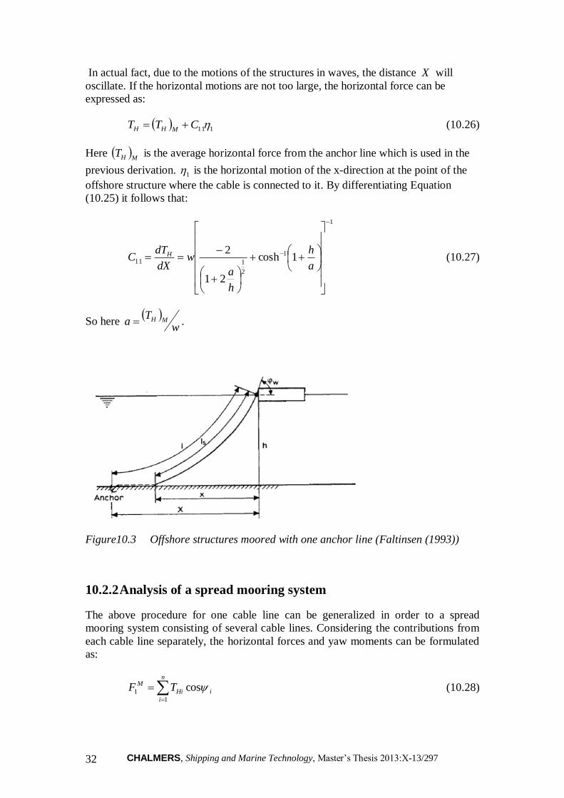
CHALMERS, Shipping and Marine Technology, Master’s Thesis 2013:X-13/297 32
In actual fact, due to the motions of the structures in waves, the distance X will
oscillate. If the horizontal motions are not too large, the horizontal force can be
expressed as:
111CTTMHH (10.26)
Here MHT is the average horizontal force from the anchor line which is used in the
previous derivation. 1 is the horizontal motion of the x-direction at the point of the
offshore structure where the cable is connected to it. By differentiating Equation
(10.25) it follows that:
1
1
2
111 1cosh
21
2
a
h
h
a
wdX
dTC H (10.27)
So here
wT
a MH .
Figure10.3 Offshore structures moored with one anchor line (Faltinsen (1993))
10.2.2 Analysis of a spread mooring system
The above procedure for one cable line can be generalized in order to a spread
mooring system consisting of several cable lines. Considering the contributions from
each cable line separately, the horizontal forces and yaw moments can be formulated
as:
n
i
iHi
M TF1
1 cos (10.28)
CHALMERS, Shipping and Marine Technology, Master’s Thesis 2013:X-13/297 33
n
i
iHi
M TF1
2 sin (10.29)
n
i
iiiiHi
M yxTF1
6 cossin (10.30)
where HiT is the horizontal force from anchor line number i . Its direction is from the
attachment point of the anchor line towards the anchor. Furthermore, ix and iy are
the x and y coordinates, respectively, of the attachment point of the anchor line to the
offshore structure and i is the angle between the anchor line and the x-axis.
The restoring coefficients of the mooring systems can be formulated as:
n
i
iikC1
2
11 cos (10.31)
n
i
iikC1
2
22 sin (10.32)
n
i
iiiii yxkC1
2
66 cossin (10.33)
10.3 Existing subroutine for a mooring system
10.3.1 Mooring stiffness calculation
The mooring line stiffness is calculated via subroutine CATMOOR. It is calculated
based on Equation (10.27) and the stiffness of the spread mooring system is calculated
via Equations (10.31)-(10.33). An initial guess of pre-tension is made at the
beginning of the subroutine and the horizontal component of the mooring line force is
approximated equal to pre-tension. A loop is established in order to optimize the
result and select a suitable mooring line. The diameter, mass and breakload of thirteen
different kinds of mooring lines are provided in the program in the subroutine
SCANROPE.
The pre-tension will increase step by step during iterations for each line until it is
lager than breakload/1.5. Subsequently, this mooring line will be substituted by
another one and repeat the above calculation. The criteria for stopping the loop is that
the static offset is smaller than 7% of the water depth and the safety factor of each
mooring line is lager than 2.7.
If the above criteria cannot be satisfied by all kinds of mooring lines, the program
will automatically choose the stiffest mooring line.

CHALMERS, Shipping and Marine Technology, Master’s Thesis 2013:X-13/297 34
10.3.2 Static offset calculation
The static offset and safety factor is calculated via the subroutine OFFSETCALC. The
environment load in the program includes wind force and current force which can be
introduced from subroutine WINDFORCE and subroutine CURRFORCE. The
stiffness of the spread mooring systems is regarded as a constant and the static offset
can be obtained as the load divided by the stiffness. It is only valid for a small offset.
The maximum line tension is calculated in the program based on Equation (10.21)
where 0z . The safety factor of each line is defined as the breakload divided by the
line tension.
10.4 A modification of the subroutine for the mooring
system
10.4.1 A modification of the subroutine for mooring stiffness
Originally, in the subroutine CATMOOR for the calculation of mooring systems, only
four angles are proposed to be the possible angle combination of mooring line
systems, which are 45˚, 135˚, 225˚ and 315˚. If the system consists of more than four
lines, the multiplicator is introduced, which is defined as the number of mooring lines
divided by 4. This multiplicator actually assumes that there will be more than one line
in the same position and sharing same angle, which is unrealistic. Especially for a yaw
motion, this assumption will lead to computation errors since yaw is sensitive to the
angle combination.
Normally considering the number of mooring lines for a semi-submersible as being
around 16, in the modified subroutine, 16 angles are proposed as the angle
combination for a mooring line system while the multiplicator is changed to the
number of mooring line divided by 16. The proposed angles are: 39˚, 43˚, 47˚, 51˚,
129˚, 133˚, 137˚, 141˚, 219˚, 223˚, 227˚, 231˚, 309˚, 313˚, 317˚ and 321˚.
10.4.2 A modification of the subroutine for a static offset
In the existing subroutine when calculating the wind and current forces which induce
the platform offset, only the wind and current coefficients for surge are introduced.
The coefficients for sway in head sea are simplified in the same as surge in beam,
while coefficients for sway in beam are same as surge in head sea. For quarter sea, it
is assumed that they have the same coefficients.
The assumptions above can result in a minor inaccuracy, so in the modified
subroutine the wind and current coefficients for both surge and sway are introduced
from subroutine WINDFORCE and subroutine CURRFORCE thus making the
current and wind force independent of each other and improving accuracy.
CHALMERS, Shipping and Marine Technology, Master’s Thesis 2013:X-13/297 35
11 The Mean Drift Force in Offset Calculation
11.1 The mean drift force on offshore structures
Environmental loads acting on offshore structures include wind, current and wave
forces. So when calculating the static offset of offshore structures, the mean drift
force should be included as part of the environmental force.
Drift force is induced by non-linear wave potential effects. The solution of the
second-order problem results in a mean drift force and a force oscillating in a low-
frequency region.
A simple example is shown here in order to explain the mean drift force. Assuming
that a regular wave hits a vertical wall and is fully reflected, the time-average force
acting on the wall can be calculated based on the following equation:
2
2
1agF (11.1)
where F is the mean drift force (time average force acting on the wall), a is the
amplitude of the incident wave. It can be seen from Equation (11.1) that when it is
fully reflected, the drift force has a magnitude proportional to the square of the
incoming wave amplitude and it is directed towards the wall, which is not the same as
a linear solution. But, generally, only a part of the regular wave will be reflected and
the rest will be transmitted underneath the floating body.
Normally, two methods can be adopted to derive the drift force: one is the
conservation of momentum and another is the direct integration method. The detailed
derivation using the direct integration method is given in Appendix 10 and here the
mean drift force of an irregular wave has been directly adopted:
dQSF WD
i
s
i ,20
(11.2)
where )(S is the P-M sea spectrum as described in Section 3.3, ,WD
iQ is the
wave drift coefficient function for direction and frequency . It can be defined as:
2
;
a
iWD
i
FQ
(11.3)
where ;iF are the mean wave loads in regular waves and a is wave amplitude.
CHALMERS, Shipping and Marine Technology, Master’s Thesis 2013:X-13/297 36
11.2 Calculation of the mean drift force in HYDA
In order to include the mean drift force when calculating the static offset of the
offshore structure, a new subroutine MEANDRIFT is established. The transfer
functions in 36 different frequency and 3 different headings are calculated via
WADAM, based on both a momentum conservation method and a direct integration
method. The results are listed in the output file wadam.fca.
In subroutine MEANDRIFT, the values of transfer functions based on the momentum
conservation method are read into the program. The expression for numerical
integration is formulated as:
36
1
111
2
,,
22
i
iii
WD
ii
WD
iiis
i
QQSSF
(11.4)
The integration is implemented in this subroutine and the mean drift force can be
obtained. Statically, the total force can be represented as the sum of the current force,
mean drift force and wind force. A new calculated static offset including the effect
from the mean drift force is saved in the file staticoffset.fca.

CHALMERS, Shipping and Marine Technology, Master’s Thesis 2013:X-13/297 37
12 Optimization of the Non-Conventional Unit
Based on the results in Section 5.3, it can be seen that the value of an objective
function is still relatively high and the amplitude of many responses do not fulfil the
requirements. In this chapter, in order to optimize the motion response and reduce the
value of the objective function, the optimization of the non-conventional unit will be
carried out in order to adjust the geometrical dimension of the platform.
12.1 Optimization algorithm
The criteria for selecting a pertinent optimization algorithm are robustness and
performance. Robustness is used in the meaning that the algorithm shall work on all
geometry types in the model library and not stop optimization unless it is stopped
manually. Performance means a high rate of convergence throughout the
optimization. Basically, it rules out gradient-based algorithms that primarily work in
the vicinity of a local minimum. According to the criteria listed above, the Simplex
method is selected and combined with a grid-based selection of start guesses.
12.2 Framework of the analysis
A deep-water floating system is an integration-dynamic system of a floater, risers and
moorings responding to wind, wave and current loading in a complex way. Thus,
different analysis methods are proposed to account for the interaction and coupled
effects between slender structures and large volume floaters become significant. In
this chapter, for the analysis of the non-conventional unit, the following analysis
method is selected.
12.2.1 Analysis domain
A frequency domain analysis is carried out in this chapter. The transfer functions are
generated in WADAM and it is the basis for frequency-dependent excitation forces
(1st and 2
nd order), added mass and damping.
12.2.2 Motion time scale
A floating moored structure may respond to environment loads on three different time
scales: wave frequency motions, low-frequency motions and high-frequency motions.
Here, in this analysis only a wave frequency motion is considered.
12.2.3 Coupling effects
Coupling effects refer to the influence on the floater mean position and dynamic
response from a slender structure restoring, damping and inertia force.
The analysis is considered to be de-coupled. The equations of the rigid body floater
motions are solved in the frequency domain. The effects of the mooring are included
CHALMERS, Shipping and Marine Technology, Master’s Thesis 2013:X-13/297 38
quasi-statically using non-linear springs. Riser effects are disregarded here. For other
coupling effects, for example contributions from damping and current loading on the
mooring line, are not considered here.
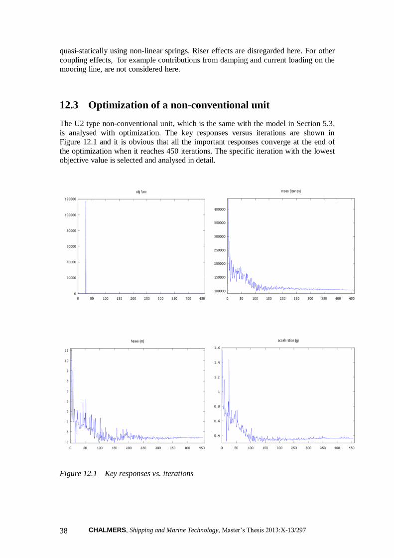
12.3 Optimization of a non-conventional unit
The U2 type non-conventional unit, which is the same with the model in Section 5.3,
is analysed with optimization. The key responses versus iterations are shown in
Figure 12.1 and it is obvious that all the important responses converge at the end of
the optimization when it reaches 450 iterations. The specific iteration with the lowest
objective value is selected and analysed in detail.
Figure 12.1 Key responses vs. iterations
CHALMERS, Shipping and Marine Technology, Master’s Thesis 2013:X-13/297 39
After optimizing the unit, optimized parameter data are collected and put as input data
for analysing the model again with a normal mode. After analysing the model, the
following important results are listed below and compared with target values.
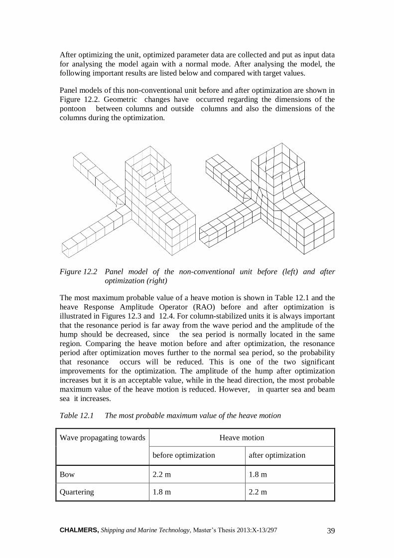
Panel models of this non-conventional unit before and after optimization are shown in
Figure 12.2. Geometric changes have occurred regarding the dimensions of the
pontoon between columns and outside columns and also the dimensions of the
columns during the optimization.
Figure 12.2 Panel model of the non-conventional unit before (left) and after
optimization (right)
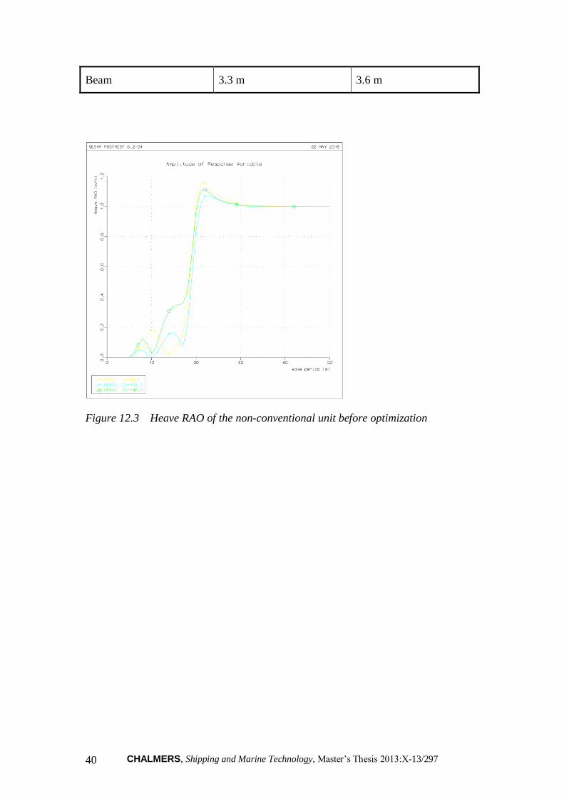
The most maximum probable value of a heave motion is shown in Table 12.1 and the
heave Response Amplitude Operator (RAO) before and after optimization is
illustrated in Figures 12.3 and 12.4. For column-stabilized units it is always important
that the resonance period is far away from the wave period and the amplitude of the
hump should be decreased, since the sea period is normally located in the same
region. Comparing the heave motion before and after optimization, the resonance
period after optimization moves further to the normal sea period, so the probability
that resonance occurs will be reduced. This is one of the two significant
improvements for the optimization. The amplitude of the hump after optimization
increases but it is an acceptable value, while in the head direction, the most probable
maximum value of the heave motion is reduced. However, in quarter sea and beam
sea it increases.
Table 12.1 The most probable maximum value of the heave motion
Wave propagating towards Heave motion
before optimization after optimization
Bow 2.2 m 1.8 m
Quartering 1.8 m 2.2 m
CHALMERS, Shipping and Marine Technology, Master’s Thesis 2013:X-13/297 40
Beam 3.3 m 3.6 m
Figure 12.3 Heave RAO of the non-conventional unit before optimization

CHALMERS, Shipping and Marine Technology, Master’s Thesis 2013:X-13/297 41
Figure 12.4 Heave RAO of the non-conventional unit after optimization
The comparison between calculation results and target values for this non-
conventional unit is listed in Table 12.2. Except for the increase of the eigenperiod
another significant improvement is the reduction of width. A dry dock can normally
construct a platform with a width of 99 metres but not 112 meters. But there are also
problems with air gap and pontoon stress. The pontoon stress shown here is just a
rough estimation, but it indicates that structural damage may occur. However, a
further detailed structural calculation is necessary in order to check the pontoon
strength since it is possible that the stress will be redistributed and the pontoon stress
will be reduced. A negative air gap may result in the wave-in-deck force, which will
be illustrated in Section 12.4.3.
Table 12.2 Comparison between calculation results and target values for the non-
conventional unit
Considered response and
geometric limits
Results from analysis model Target value
Start guess Optimized
Offset amplitude (% of water
depth)
6.7 6.5 7.0
Heel amplitude (˚) 3.9 4.2 5.5
Heave amplitude (m) 3.3 3.6 2.0
Metacentric height (m) 13.2 1.6 2.0

CHALMERS, Shipping and Marine Technology, Master’s Thesis 2013:X-13/297 42
Air-gap (m) -7.2 -2.4 1.5
Acceleration (g) 0.66 0.74 0.15
Total mass ( 310 tonnes) 59 75 10
Pontoon stress (MPa) 1825 892 150
Eigenperiod associated with
heave motion (s)
19.8 21.2 22
Draught (m) 30 30 30
Width (m) 112 99 80
It is clear that after optimization there is a great improvement in width reduction and
a reasonable improvement in air-gap and eigenperiod. But in the maximum heave
amplitude, the improvement even increases in the quarter and beam direction, while
it deceases in the head direction. Now it is necessary to make sure that these are
values that are improved compared to a traditional conventional unit with the same
environmental and geometri conditions. After comparing, it can be concluded that
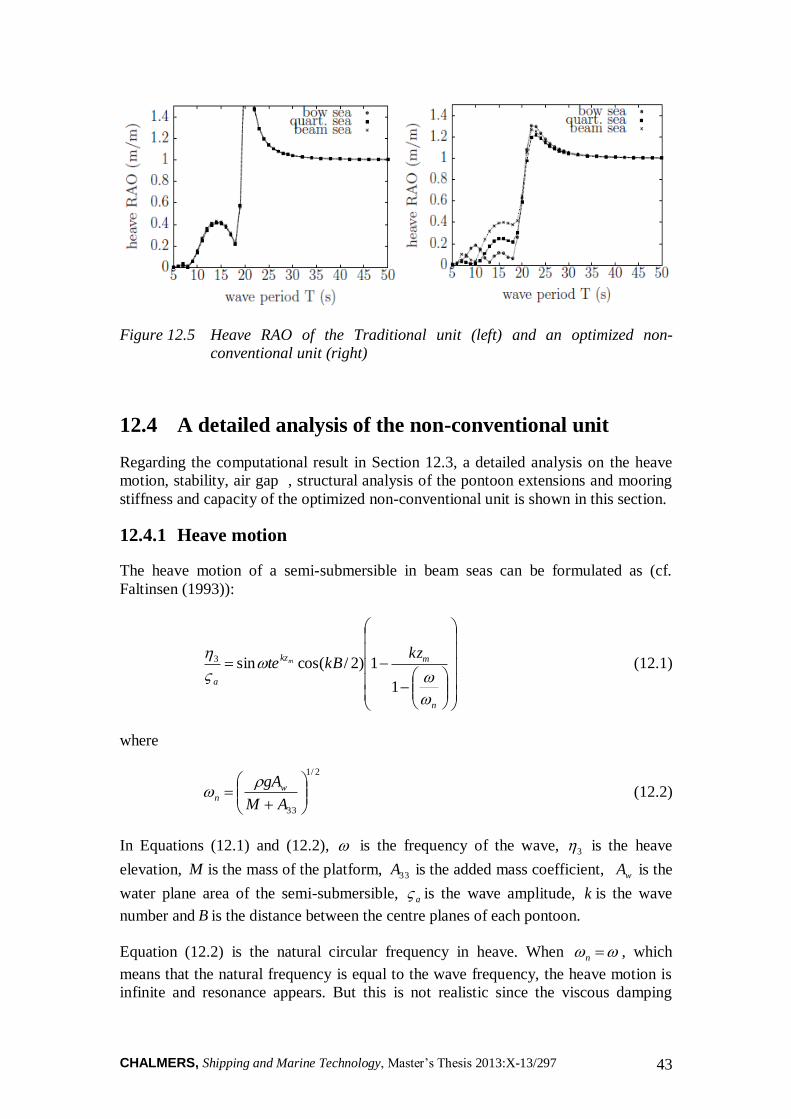
this non-conventional unit can give a better result in a heave motion. Figure 12.5
shows that in quarter sea and beam sea, the amplitude of the hump is reduced
significantly. The most maximum probable value of the heave motion is shown in
Table 12.3.
Table 12.3 Most probable maximum value of the heave motion
Wave propagating towards Heave motion
Traditional unit Non-conventional unit
Bow 4.7 m 1.8 m
Quartering 4.6 m 2.2 m
Beam 4.7 m 3.6 m
CHALMERS, Shipping and Marine Technology, Master’s Thesis 2013:X-13/297 43
Figure 12.5 Heave RAO of the Traditional unit (left) and an optimized non-
conventional unit (right)
12.4 A detailed analysis of the non-conventional unit
Regarding the computational result in Section 12.3, a detailed analysis on the heave
motion, stability, air gap , structural analysis of the pontoon extensions and mooring
stiffness and capacity of the optimized non-conventional unit is shown in this section.
12.4.1 Heave motion
The heave motion of a semi-submersible in beam seas can be formulated as (cf.
Faltinsen (1993)):
n
mkz
a
kzkBte m
1
1)2/cos(sin3 (12.1)
where
2/1
33
AM
gAwn
(12.2)
In Equations (12.1) and (12.2), is the frequency of the wave, 3 is the heave
elevation, M is the mass of the platform, 33A is the added mass coefficient, wA is the
water plane area of the semi-submersible, a is the wave amplitude, k is the wave
number and B is the distance between the centre planes of each pontoon.
Equation (12.2) is the natural circular frequency in heave. When n , which
means that the natural frequency is equal to the wave frequency, the heave motion is
infinite and resonance appears. But this is not realistic since the viscous damping
CHALMERS, Shipping and Marine Technology, Master’s Thesis 2013:X-13/297 44
effect is neglected. In reality, it is shown as in Figures 12.3 and 12.4 that when the
wave period is close to the eigenperiod, the heave amplitude becomes very large.
The heave motion can be considered the resultant of two principal components. The
first component is the response to the oscillatory forces exerted by the wave on the
columns. The second component is the response to the oscillatory forces acting on the
pontoons. For a non-conventional unit, the force on the pontoon can be partially
cancelled due to the outboard extension. This will be shown in the following:
Assume that a wave passes through a semi-submersible and the wave crest appears at
the centre of the platform. Based on potential theory and the Bernoulli equation, the
dynamic pressure induced by waves can be derived as:
gzwtkxgaep kz cos (12.3)
From Equation (12.3) it can be seen that a wave crest gives a higher pressure. That is
why, in a semi-submersible, different part of the pontoons contribute unequally to the
total dynamic pontoon force when analysed with respect to a wave crest appearing at
the centre of the semi-submersible. In particular, the inboard portions contribute more
dynamic force per volume because they are at the wave crest while the outboard
portions contribute less dynamic force per volume because they are located near the
wave troughs.
But as described in Section 5.3, there is an outboard extension with a suitable length
for the non-conventional unit, which can partially but not totally cancel the dynamic
force on the pontoon. Consequently, in the presence of a wave crest, the total dynamic
force on both pontoon and column can be reduced, thereby reducing the heave
motion. If the length of the outboard extension is not appropriate, a possible result is
that it will totally cancel the dynamic force on the pontoon and thus the force on the
column will be dominant, which is unexpected.
12.4.2 Stability
For operational conditions, the metacentric height before optimization is 2.13lGM
m and 2.13tGM m in the longitudinal and transverse direction, respectively. But
the metacentric height for the optimized platform is 6.1tGM m and 86.2lGM m,
which decreases significantly. This is mainly due to the shift of the centre of gravity.
The metacentric height after optimization is slightly low for a robust design and
further investigation could be made to increase it.
12.4.3 Air gap
A positive air gap should generally be ensured including the relative motion of the
platform and interaction effects (cf. DNV (2008)). A negative air gap may be
considered as being acceptable for overhanging structures and appendages to the deck
structure. The response spectrum of the relative motion r is calculated as follows:
zer 2.1 (12.4)

CHALMERS, Shipping and Marine Technology, Master’s Thesis 2013:X-13/297 45
Where denotes the angular frequency, e denotes the wave crest and z denotes the
absolute motion of the studied location. Moreover, the purpose of the factor 1.2 in
Equation (12.4) is to account for deviations from an ideal sinusoidal wave for semi-
submersibles or TLP (cf. DNV (2010)). The most probable maximum rX is
calculated from the spectrum r , whereby the most probable minimum air gap is
calculated by subtracting rX from the static air gap .
The target value of the most probable minimum air gap is set to 1.5 m considering
operational aspects and requirements for inspection and maintenance. But the air gap
for an optimized value is -2.4 m. This negative value may result in the wave impact
on deck and this wave impact should be taken into fully account in the structural
design and it may lead to structural failure.
12.4.4 Structural analysis of pontoon extensions
In Figure 12.2 it is seen that the optimization result gives wide but short pontoon
extensions, which may cause problems in structure strength. Thus, in this section, a
rough evaluation with respect to shear strength of the extensions is shown below.
The sea pressures attacking the extensions can be estimated as (cf. DNV (2008)):
370/2 zgaegzp kPa (12.5)
where draught 30z m, 14 sHa m, 321s m. The first term in Equation (12.5)
is static pressure and the second term is dynamic wave pressure. The shear force can
be obtained by integrating pressure in the upper surface of the extension:
146
pSdspV MN (12.6)
where S is the upper surface of the extension, and can be calculated by:
1413 ssS 396 m2 (12.7)
13s and 14s are defined in Appendix 2.
The side plating and the interior bulkhead is exposed to shearing due to loadingV .
The shear stress in the bulkhead is estimated as:
6812
ht
V MPa (12.8)
where 15h m and 12t mm, the minimum thickness of the plating.
The design yield strength 308ydf MPa corresponding to a high-strength steel NV-
36 is assumed. Then the safety margin for shear strength is 1773/ ydyd f MPa.
The safety factor 6.11/ yds .

CHALMERS, Shipping and Marine Technology, Master’s Thesis 2013:X-13/297 46
12.4.5 Mooring stiffness and capacity
Mooring stiffness depends on pre-tension , the mass of mooring line, type of rope,
water depth and spreading. The stiffness of a spread mooring system is considered in
surge, sway, yaw and the equations of the stiffness are described in Equations (10.31),
(10.32) and (10.33). Results of mooring stiffness in different components are shown
in Table 12.4.
Table 12.4 Mooring stiffness of the non-conventional unit
Component Stiffness
surge-surge C11 =99 kN/m
sway-sway C22 =99 kN/m
yaw-yaw C66 =2996 MNm/radians
The mooring capacity is presented in terms of factors of safety, and the factors of
safety are defined as a ratio of break load and maximum line tension. To calculate the
static offset, it is assumed that the wind direction and current direction coincide and
the static offset is calculated from the following formula:
%10022
waterdepth
swaysurgeetstaticoffs (12.9)
The target value of the static offset is lower than 7% and the safety factor is greater
than 2.7. In this analysis, the static offset in the bow and beam direction fulfil the
target value as shown in Table 12.5, while the safety factor of the lines are presented
in Table 12.6, and the safety factor for all mooring lines in all directions also fulfil the
target value.
Table 12.5 Static offset of the non-conventional unit
Wind and current
propagating towards
Surge (m) Sway (m) 100
22
waterdepth
swaysurge%
Bow 32 0 6.5
Quartering 25 25 7.2
Beam 0 32 6.5
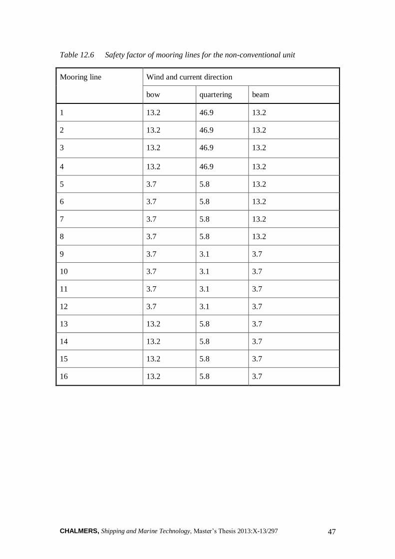
CHALMERS, Shipping and Marine Technology, Master’s Thesis 2013:X-13/297 47
Table 12.6 Safety factor of mooring lines for the non-conventional unit
Mooring line Wind and current direction
bow quartering beam
1 13.2 46.9 13.2
2 13.2 46.9 13.2
3 13.2 46.9 13.2
4 13.2 46.9 13.2
5 3.7 5.8 13.2
6 3.7 5.8 13.2
7 3.7 5.8 13.2
8 3.7 5.8 13.2
9 3.7 3.1 3.7
10 3.7 3.1 3.7
11 3.7 3.1 3.7
12 3.7 3.1 3.7
13 13.2 5.8 3.7
14 13.2 5.8 3.7
15 13.2 5.8 3.7
16 13.2 5.8 3.7
CHALMERS, Shipping and Marine Technology, Master’s Thesis 2013:X-13/297 48
13 Concluding Remarks
HYDA is a powerful tool and can perform state-of-the-art analysis for thye design and
optimization of different types of floating platforms. As clarified in the objective,
there are two parts in the project: modification of software HYDA and optimization of
the non-conventional unit.
For the first part of the project, after modification one more reference model is taken
into consideration and piecewise functions are adopted in order to give a more
accurate estimation for mass budget scaling. The superstructure and area of facilities
on deck are included in the projected area of platforms for wind-force scaling.
Moreover, similar to mass budget scaling, one more reference model is introduced
and piecewise functions are adopted in wind-force scaling. Current force scaling for a
sway and roll response is modified, while for surge and pitch it is kept unchanged. In
the mooring stiffness calculation the number of possible mooring angle combinations
is increased and the mean wave-drift force is included in the static offset calculation.
So for this part the goal has been reached.
For the second part, the optimization of a non-conventional unit is assessed using
HYDA, and the motion response before and after optimization is compared and
analysed. From the comparison it is concluded that the width of the platform after
optimization is significantly reduced while the eigenperiod increases. Both of the non-
conventional units before and after optimization give a good result in the heave
motion - considerably reduced compared to a conventional unit. But problems appear
with air gap and pontoon stress. A negative air gap appears and a high pontoon
stress may result in structure damage. So, the goal of this second part has not been
fully realized because the optimization procedure is complicated and depends on
several weighting factors. Further investigation is necessary on the optimization of a
non-conventional unit in order to achieve a platform with good performance in all
the considered responses.
CHALMERS, Shipping and Marine Technology, Master’s Thesis 2013:X-13/297 49
14 References
G. Bergman (1978): Heave stabilization of semi-submersible platforms. United States
patent, 4112864, Montecito, California, 63-65 pp.
O. M. Faltinsen (1993): Sea loads on ships and offshore structures. Cambridge
University Press, Cambridge.
DNV (2008): Structural design of column stabilized units (LRFD method), Sec.4,
DET NORSKE VERITAS AS, DNV-OS-C103, Oslo, Norway, 17 pp.
DNV (2010): Environmental conditions and environmental loads, Sec.4, DET
NORSKE VERITAS AS, DNV-RP-C205, Oslo, Norway, 76-77 pp.
Journee, J.M.J. and Massie, W.W. (2001): Offshore hydromechanics, Delft University
of Technology, Delft, Netherland.
DNV (2010): Global performance analysis of deepwater floating structures, DET
NORSKE VERITAS AS, DNV-RP-F205, Oslo, Norway, 8-9 pp.
NORSOK (2010): Actions and action effects, Standard Norway, NORSOK
STANDARD N-003, Oslo, Norway, 45-46 pp.
MARINTEK (2010): MIMOSA 6.3-User’s Documentation, Norwegian Marine
Technology Research Institute, Trondheim, Norway, 22-23 pp.
DNV (2010): Position mooring, Sec.4. DET NORSKE VERITAS AS, DNV-OS-E103,
Oslo, Norway, 29-31 pp.
API (2005): Design and analysis of stationkeeping systems for floating structures,
American Petroleum Institute, Washington, American, 15-18 pp.
DNV (2007): SESAM User Manual POSTRESP, DET NORSKE VERITAS AS, Oslo,
Norway.
DNV (2008): SESAM User Manual WADAM, DET NORSKE VERITAS AS, Oslo,
Norway.
CHALMERS, Shipping and Marine Technology, Master’s Thesis 2013:X-13/297 50
Appendix 1: Revision and Update History of HYDA
Program package: HYDA Created by: GJ January 2011 Purpose to create: aid in design of floating production platforms Purpose to modify: refine some of the subroutines with regard to mass
budget, wind-force scaling, current force scaling, mooring systems and static offset.
Modified by: Hao and Mezbah April 2013
Subroutines: DEFAULTPARAM and READINPUTFILE Purpose to create: set start parameter values Created by: GJ January 2011 Purpose to modify: make the subroutine correspond to modified input
file Modified by: Hao and Mezbah April 2013 Called by: main program HYDA
Subroutine: MASSBUDGET Purpose to create: estimate mass budget
Created by: GJ January 2011 Called by: main program HYDA Overall check of semi equipment list by: GJ 10 August 2011 Purpose to modify: introduce a flag to define a reference model
(predefined or user-defined) Modified by: Hao and Mezbah April 2013
Subroutine: EQUIPMENTLIST1 Purpose to create: scale mass budget for model type 1
Created by: GJ January 2011 Called by: Subroutine MASSBUDGET Purpose to modify: introduce two reference models to estimate the
mass budget Modified by: Hao and Mezbah April 2013
Subroutine: EQUIPMENTLIST3 Purpose to create: scale mass budget for model type 3
Created by: GJ January 2011 Called by: Subroutine MASSBUDGET
Subroutine: EQUIPMENTLIST4 Purpose to create: scale mass budget for model type 4
Created by: GJ January 2011 Called by: Subroutine MASSBUDGET
Subroutine: EQUIPMENTLIST5 Purpose to create: scale mass budget for model type 5
Created by: GJ January 2011

CHALMERS, Shipping and Marine Technology, Master’s Thesis 2013:X-13/297 51
Called by: Subroutine MASSBUDGET
Subroutine: EQUIPMENTLIST9 Purpose to create: scale mass budget for model type 9
Created by: GJ January 2011 Called by: Subroutine MASSBUDGET
Subroutine: EQUIPMENTLIST12 Purpose to create: scale mass budget for model type 12
Created by: GJ January 2011 Called by: Subroutine MASSBUDGET
Subroutine: MASSCALCULATION Purpose to create: calculate total mass and radii of gyration
Created by: GJ January 2011 Called by: Subroutine MASSBUDGET
Subroutine: PGENIE Purpose to create: create panel model
Created by: GJ Mars 2011 Called by: main program HYDA
Subroutine: PGENIE1 Purpose to create: generate model type 1
Created by: GJ Mars 2011 Called by: Subroutine PGENIE
Subroutine: PGENIE2 Purpose to create: generate model type 2 Created by: GJ Mars 2011 Called by: Subroutine PGENIE
Subroutine: PGENIE3 Purpose to create: generate model type 3 Created by: GJ Mars 2011 Called by: Subroutine PGENIE
Subroutine: PGENIE4 Purpose to create: generate model type 4 Created by: GJ Mars 2011 Called by: Subroutine PGENIE
Subroutine: PGENIE5 Purpose to create: generate model type 5 Created by: GJ Mars 2011 Called by: Subroutine PGENIE
Subroutine: PGENIE6 Purpose to create: generate model type 6 Created by: GJ Mars 2011
CHALMERS, Shipping and Marine Technology, Master’s Thesis 2013:X-13/297 52
Called by: Subroutine PGENIE
Subroutine: PGENIE7 Purpose to create: generate model type 7 Created by: GJ Mars 2011 Called by: Subroutine PGENIE
Subroutine: PGENIE8 Purpose to create: generate model type 8 Created by: GJ Mars 2011 Called by: Subroutine PGENIE
Subroutine: PGENIE9 Purpose to create: generate model type 9 Created by: GJ Mars 2011 Called by: Subroutine PGENIE
Subroutine: PGENIE10 Purpose to create: generate model type 10 Created by: GJ Mars 2011 Called by: Subroutine PGENIE
Subroutine: PGENIE11 Purpose to create: generate model type 11 Created by: GJ Mars 2011 Called by: Subroutine PGENIE
Subroutine: PGENIE12 Purpose to create: generate model type 12 Created by: GJ Mars 2011 Called by: Subroutine PGENIE
Subroutine: PGENIE13 Purpose to create: generate model type 13 Created by: GJ Mars 2011 Called by: Subroutine PGENIE
Subroutine: PGENIE14 Purpose to create: generate model type 14 Created by: GJ Mars 2011 Called by: Subroutine PGENIE
Subroutine MORISON Purpose to create: create slender element model Created by: GJ Mars 2011 Called by: main program HYDA
Subroutine CATMOOR Purpose to create: calculate catenary mooring stiffness Created by: GJ 15 Mars 2011
CHALMERS, Shipping and Marine Technology, Master’s Thesis 2013:X-13/297 53
Purpose to modify: change the angle combination of mooring lines Modified by: Hao and Mezbah April 2013 Called by: main program HYDA
Subroutine STATICOFFSET Purpose to create: calculating static offset
Created by: GJ Mars 2011 Purpose to modify: introduce environment load in an accurate way Modified by: Hao and Mezbah April 2013 Called by: main program HYDA
Subroutine PREFEM Purpose to create: generation of post-script figures
Created by: GJ Mars 2011 Called by: main program HYDA
Subroutine: WINDFORCE Purpose to create: estimate wind-force coefficients
Created by: GJ April 2011 Called by: main program HYDA Overall check by: GJ August 2011 Comparative check by: GJ August 2011 Purpose to modify: introduce experiment data from wind tunnel;
consider the above area of platforms, which may have an effect on wind resistance
Modified by: Hao and Mezbah April 2013
Subroutine: CURRFORCE Purpose to create: estimate current force coefficients
Created by: GJ April 2011 Called by: main program HYDA Overall check by: GJ August 2011 Comparative check by: GJ August 2011 Purpose to modify: modify the typical dimensions of the platforms used
in the formula for estimating current resistance Modified by: Hao and Mezbah April 2013
Subroutine: OBJECTFUNC Purpose: calculate object function to minimize Created by: GJ April 2011 Called by: main program HYDA Overall check by: GJ August 2011
Subroutine CHECKPARAM Purpose: check for conflicts between parameters Created by: GJ May 2011 Called by: main program HYDA
Subroutine STRUCPONTOON Purpose: assess strength of pontoon

CHALMERS, Shipping and Marine Technology, Master’s Thesis 2013:X-13/297 54
Created by: GJ May 2011 Called by: main program HYDA
Subroutine CASH Purpose: calculate non-linear and low-frequent responses Created by: GJ May 2011 Called by: main program HYDA Calls: external program CASH
Subroutine GM
Purpose: calculate GZ-curve
Created by: GJ June 2012 Called by: main program HYDA Calls: external program READLIS
Subroutine READWADAMLIS Purpose: read basis properties from WADAM result list Created by: GJ June 2012 Called by: main subroutine GM among others
Subroutine MEANDRIFT Purpose to create: calculate mean drift force and calculate the static
offset again including the mean drift force Created by: Hao and Mezbah April 2013 Called by: main program HYDA
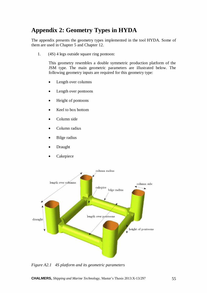
CHALMERS, Shipping and Marine Technology, Master’s Thesis 2013:X-13/297 55
Appendix 2: Geometry Types in HYDA
The appendix presents the geometry types implemented in the tool HYDA. Some of
them are used in Chapter 5 and Chapter 12.
1. (4S) 4 legs outside square ring pontoon:
This geometry resembles a double symmetric production platform of the
JSM type. The main geometric parameters are illustrated below. The
following geometry inputs are required for this geometry type:
Length over columns
Length over pontoons
Height of pontoons
Keel to box bottom
Column side
Column radius
Bilge radius
Draught
Cakepiece
Figure A2.1 4S platform and its geometric parameters
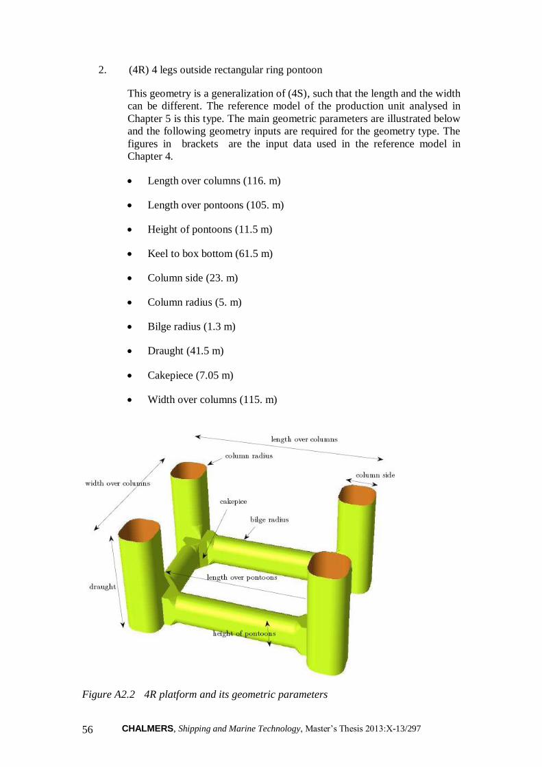
CHALMERS, Shipping and Marine Technology, Master’s Thesis 2013:X-13/297 56
2. (4R) 4 legs outside rectangular ring pontoon
This geometry is a generalization of (4S), such that the length and the width
can be different. The reference model of the production unit analysed in
Chapter 5 is this type. The main geometric parameters are illustrated below
and the following geometry inputs are required for the geometry type. The
figures in brackets are the input data used in the reference model in
Chapter 4.
Length over columns (116. m)
Length over pontoons (105. m)
Height of pontoons (11.5 m)
Keel to box bottom (61.5 m)
Column side (23. m)
Column radius (5. m)
Bilge radius (1.3 m)
Draught (41.5 m)
Cakepiece (7.05 m)
Width over columns (115. m)
Figure A2.2 4R platform and its geometric parameters
CHALMERS, Shipping and Marine Technology, Master’s Thesis 2013:X-13/297 57
The primary input used in the reference model of the production unit in
Chapter 5 is listed below:
Topside mass (28444 tonnes)
Riser mass (10707 tonnes)
Umbilical mass (2460 tonnes)
Water depth (2130 m)
Significant wave height (14.70 m)
Min peak period (11.00 s)
Max peak period (14.80 s)
Wind velocity, one hour average at 10 m altitude (39.0 m/s)
Surface current (1.58 m/s)
Number of equally spread mooring lines (16)

CHALMERS, Shipping and Marine Technology, Master’s Thesis 2013:X-13/297 58
3. (S4) Square ring pontoon under 4 circular legs
This double symmetric geometry is similar to (4S). The main geometric
parameters are illustrated below and the following geometry inputs are
required for this geometry type:
Length over columns
Height of pontoons
Keel to box bottom
Column side
Draught
Cakepiece
Figure A2.3 S4 platform and its geometric parameters
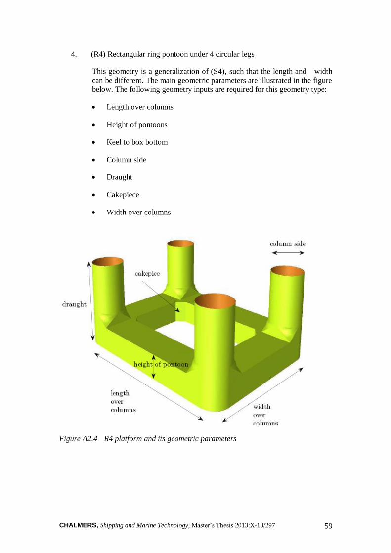
CHALMERS, Shipping and Marine Technology, Master’s Thesis 2013:X-13/297 59
4. (R4) Rectangular ring pontoon under 4 circular legs
This geometry is a generalization of (S4), such that the length and width
can be different. The main geometric parameters are illustrated in the figure
below. The following geometry inputs are required for this geometry type:
Length over columns
Height of pontoons
Keel to box bottom
Column side
Draught
Cakepiece
Width over columns
Figure A2.4 R4 platform and its geometric parameters
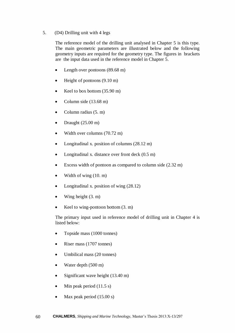
CHALMERS, Shipping and Marine Technology, Master’s Thesis 2013:X-13/297 60
5. (D4) Drilling unit with 4 legs
The reference model of the drilling unit analysed in Chapter 5 is this type.
The main geometric parameters are illustrated below and the following
geometry inputs are required for the geometry type. The figures in brackets
are the input data used in the reference model in Chapter 5.
Length over pontoons (89.68 m)
Height of pontoons (9.10 m)
Keel to box bottom (35.90 m)
Column side (13.68 m)
Column radius (5. m)
Draught (25.00 m)
Width over columns (70.72 m)
Longitudinal x. position of columns (28.12 m)
Longitudinal x. distance over front deck (0.5 m)
Excess width of pontoon as compared to column side (2.32 m)
Width of wing (10. m)
Longitudinal x. position of wing (28.12)
Wing height (3. m)
Keel to wing-pontoon bottom (3. m)
The primary input used in reference model of drilling unit in Chapter 4 is
listed below:
Topside mass (1000 tonnes)
Riser mass (1707 tonnes)
Umbilical mass (20 tonnes)
Water depth (500 m)
Significant wave height (13.40 m)
Min peak period (11.5 s)
Max peak period (15.00 s)
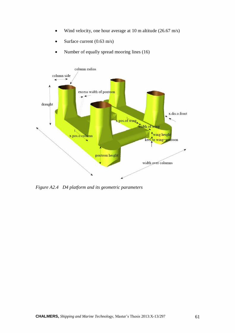
CHALMERS, Shipping and Marine Technology, Master’s Thesis 2013:X-13/297 61
Wind velocity, one hour average at 10 m altitude (26.67 m/s)
Surface current (0.63 m/s)
Number of equally spread mooring lines (16)
Figure A2.4 D4 platform and its geometric parameters
CHALMERS, Shipping and Marine Technology, Master’s Thesis 2013:X-13/297 62
6. (U2) ugly production unit with 4 legs and box appendices
The U2 type is adopted in the reference model of the non-conventional unit
in Chapter 5. The following geometry inputs are required for this type of
geometry:
Longitudinal x. position of wing (47.5 m)
Pontoon height (13. m)
Length over pontoons (95. m)
Pontoon width (11. m)
Width of wing (11. m)
Cakepiece side (2. m)
Column side (21.m)
2nd column side (21. m)
Draught (38. m)
Front height (25. m)
X. displacement of front (15. m)
Front width (10. m)
Keel to box bottom (63. m)
The primary input used in reference model of non-conventional unit in
Chapter 4 is listed below:
Topside mass (33000 tonnes)
Water depth (2130 m)
Significant wave height (14.7 m)
Min peak period (11. s)
Max peak period (14.80 s)
Wind velocity, one hour average at 10 m altitude (39.0 m/s)
Surface current (1.58 m/s)
Number of equally spread mooring lines (16)

CHALMERS, Shipping and Marine Technology, Master’s Thesis 2013:X-13/297 63
Figure A2.5 U2 platform and its geometric parameters
CHALMERS, Shipping and Marine Technology, Master’s Thesis 2013:X-13/297 64
Appendix 3: Existing Mass Budget Scaling
Item of the floating platform Mass scaling
Topside Directly input data
Risers bow 4/R
Risers stern 4/R
Risers starboard 4/R
Risers port side 4/R
Equipment 33000/80 T
Umbilical Directly input data
Management reserve T1862.0
Ballast pontoon Directly input data
Ballast column 0
Fuil oil 5.41/2174 D
Portable water 5.41/1087 D
Bow starboard 33000/1927 T
Bow port 33000/1927 T
Stern port side 33000/1927 T
Stern starboard 33000/1927 T
Pontoon bow 5.185.11105/3560 pspp WHW
Pontoon stern 5.185.11105/3560 pspp WHW
Pontoon starboard 5.185.11105/3560 pspp WHW
Pontoon port side 5.185.11105/3560 pspp WHW
Column bow starboard 223.245.61/4100 cag LD
CHALMERS, Shipping and Marine Technology, Master’s Thesis 2013:X-13/297 65
Column bow port side 223.245.61/4100 cag LD
Column stern starboard 223.245.61/4100 cag LD
Column stern port side 223.245.61/4100 cag LD
Deck box 27000/13160 T
Deck house 27000/2160 T
Equipment in hull 27000/500 T
CHALMERS, Shipping and Marine Technology, Master’s Thesis 2013:X-13/297 66
Appendix 4: Modified Mass Budget Scaling
Item of the
floating
platform
Mass scaling
Equipment T<T1 T>T2 T1<T<T2
TT
EE
0
0
1
1 2
2
2
1arctan/2 E
ssT
TEEE ul
11
12
12 ETTTT
EEE
Manageme
nt reserve
T0.1862
Fuil oil D<D1 D>D2 D1<D<D2
DD
FF
0
0
1
1
2
2
2
1arctan/2 F
ssD
DFFF ul
11
12
12 FDDDD
FFF
Portable
water
D<D1 D>D2 D1<D<D2
DD
PP
0
0
1
1
2
2
2
1arctan/2 P
ssD
DPPP ul
11
12
12 PDDDD
PPP
Bow
starboard
T<T1 T>T2 T1<T<T2
TT
BB
0
0
1
1
2
2
2
1arctan/2 B
ssT
TBBB ul
11
12
12 BTTTT
BBB
Bow port T<T1 T>T2 T1<T<T2
TT
BB
0
0
1
1
2
2
2
1arctan/2 B
ssT
TBBB ul
11
12
12 BTTTT
BBB
Stern port
side
T<T1 T>T2 T1<T<T2
TT
BB
0
0
1
1
2
2
2
1arctan/2 B
ssT
TBBB ul
11
12
12 BTTTT
BBB
Stern T<T1 T>T2 T1<T<T2

CHALMERS, Shipping and Marine Technology, Master’s Thesis 2013:X-13/297 67
starboard
TT
BB
0
0
1
1
2
2
2
1arctan/2 B
ssT
TBBB ul
11
12
12 BTTTT
BBB
Pontoon
bow
Va<Va1 Va>Va2 Va1< Va<Va2
a
a
VV
MM
0
0
1
1
2
2
2
1arctan/2 M
ssV
VMMM
a
aul
11
12
12 MVVVV
MMM aa
aa
Pontoon
stern
Va<Va1 Va>Va2 Va1< Va<Va2
a
a
VV
MM
0
0
1
1
2
2
2
1arctan/2 M
ssV
VMMM
a
aul
11
12
12 MVVVV
MMM aa
aa
Pontoon
starboard
Va<Va1 Va>Va2 Va1< Va<Va2
a
a
VV
MM
0
0
1
1
2
2
2
1arctan/2 M
ssV
VMMM
a
aul
11
12
12 MVVVV
MMM aa
aa
Pontoon
port side
Va<Va1 Va>Va2 Va1< Va<Va2
a
a
VV
MM
0
0
1
1
2
2
2
1arctan/2 M
ssV
VMMM
a
aul
11
12
12 MVVVV
MMM aa
aa
Column
bow
starboard
Vc<Vc1 Vc>Vc2 Vc1< Vc<Vc2
c
c
VV
CC
0
0
1
1
2
2
2
1arctan/2 C
ssV
VCCC
c
cul
11
12
12 CVVVV
CCC cc
cc
Column
bow port
side
Vc<Vc1 Vc>Vc2 Vc1< Vc<Vc2
c
c
VV
CC
0
0
1
1
2
2
2
1arctan/2 C
ssV
VCCC
c
cul
11
12
12 CVVVV
CCC cc
cc
Column
stern
starboard
Vc<Vc1 Vc>Vc2 Vc1< Vc<Vc2
c
c
VV
CC
0
0
1
1
2
2
2
1arctan/2 C
ssV
VCCC
c
cul
11
12
12 CVVVV
CCC cc
cc
Column Vc<Vc1 Vc>Vc2 Vc1< Vc<Vc2

CHALMERS, Shipping and Marine Technology, Master’s Thesis 2013:X-13/297 68
stern port
side c
c
VV
CC
0
0
1
1
2
2
2
1arctan/2 C
ssV
VCCC
c
cul
11
12
12 CVVVV
CCC cc
cc
Deck box T<T1 T>T2 T1<T<T2
TT
II
0
0
1
1 2
2
2
1arctan/2 I
ssT
TIII ul
11
12
12 ITTTT
III
Deck
house
T<T1 T>T2 T1<T<T2
TT
JJ
0
0
1
1
2
2
2
1arctan/2 J
ssT
TjJJ ul
11
12
12 JTTTT
JJJ
Equipment
in hull
T<T1 T>T2 T1<T<T2
TT
KK
0
0
1
1
2
2
2
1arctan/2 K
ssT
TKKK ul
11
12
12 KTTTT
KKK
CHALMERS, Shipping and Marine Technology, Master’s Thesis 2013:X-13/297 69
Appendix 5: Existing Wind Force Coefficient Scaling
Motion
response
Head wind Quarter wind Beam wind
Surge force
coefficient
)/( 22 mkNs
)10519/(
58.4
SAGWp
)10519/(
5.3
SAGWp
0
Pitch moment
coefficient
)/( 2 mkNs
)10519/(04.2
58.4 2
SAGWp
)10519/(04.2
5.3 2
SAGWp
0
Sway force
coefficient
)/( 22 mkNs
0
p
p
p
W
L
SAGW
))10519/(
5.3(
p
p
p
W
L
SAGW
))10519/(
58.4(
Roll moment
coefficient
)/( 2 mkNs
0
p
p
p
W
L
SAGW
))10519/(04.2
5.3( 2
p
p
p
W
L
SAGW
))10519/(04.2
58.4( 2

CHALMERS, Shipping and Marine Technology, Master’s Thesis 2013:X-13/297 70
Appendix 6: Modified Wind-Force Coefficient Scaling
Motion response Head wind Quarter wind Beam wind
Surge
force
coefficient
)/
(
2
2
m
kNs
Af<Af1 f
f
susu A
A
HH
0
0
1
1 f
f
ss A
A
0
0
1
1 0
Af>Af2
2
2
2
1arctan
/2
su
f
f
susulsu
HssA
A
HHH
2
2
2
1arctan
/2
s
f
f
ssuls
QssA
A
QQQ
0
Af1<
Af<Af2
11
12
12
suff
ff
susu
su HAAAA
HHH
11
12
12sff
ff
sss QAA
AA
QQQ
0
Pitch
moment
coefficient
)/
( 2
m
kNs
Af<Af1
72.1
0
0
1
1
SAG
AA
HH f
f
sup
51.1
0
0
1
1
SAG
AA
QQ f
f
sp
0
Af>Af2
72.1
1arctan
/2
2
2
2
SAG
HssA
A
HHH
su
f
f
susulp
51.1
1arctan
/2
2
2
2
SAG
QssA
A
QQQ
s
f
f
ssulp
0
Af1<
Af<Af2
72.11
1
12
12
SAGH
AAAA
HHH
su
ff
ff
susu
p
51.11
1
12
12
SAGQ
AAAA
QQQ
s
f
ff
ssp
0
Sway
force
coefficient
)/
(
2
2
m
kNs
As<As1 0 s
s
swsw A
A
0
0
1
1 s
s
swsw A
A
HB
0
0
1
1
As>As2 0
2
2
2
1arctan
/2
sw
s
s
swswulsw
QssA
A
QQQ
2
2
2
1arctan
/2
sw
s
s
swswulsw
HssA
A
HHB
As1<
As<As2
0
1
1
12
12
sw
ss
ss
swswsw
Q
AAAA
QQQ
1
1
12
12
sw
ss
ss
swswsw
H
AAAA
HHB

CHALMERS, Shipping and Marine Technology, Master’s Thesis 2013:X-13/297 71
Roll
moment
coefficient
)/
( 2
m
kNs
As<As1 0
51.1
0
0
1
1
SAG
AA
QQ s
s
swr
72.1
0
0
1
1
SAG
AA
HB s
s
swr
As>As2 0
51.1
1arctan
/2
2
2
2
SAG
QssA
A
QQQ
sw
s
s
swswulr
72.1
1arctan
/2
2
2
2
SAG
HssA
A
HHB
sw
s
s
swswulr
As1<
As<As2
0
51.11
1
12
12
SAGQ
AAAA
QQQ
sw
ss
ss
swswr
72.11
1
12
12
SAGH
AAAA
HHB
sw
ss
ss
swswr
CHALMERS, Shipping and Marine Technology, Master’s Thesis 2013:X-13/297 72
Appendix 7: Drag Coefficient dC´ on Pontoons and
Columns (cf. DNV (2010))
dl
dr dC
<0.75 <0.0105 2.5
0.0105-0.053 2.2
0.053-0.1665 1.9
>0.1665 1.6
0.75-1.5 <0.0105 2.2
0.0105-0.094 2.0
0.094-0.25 1.2
>0.25 1.0
1.5-4.0 <0.021 1.6
0.021-0.1045 1.4
0.1045-0.3335 0.7
>0.3335 0.4
>4.0 <0.25 0.89
>0.25 0.29
Figure A7.1 Definition of l, r and d for a rectangular with rounded corners
CHALMERS, Shipping and Marine Technology, Master’s Thesis 2013:X-13/297 73
Appendix 8: Existing Current Force Coefficient
Scaling
Motion
response
Head Current Quarter current Beam current
Surge force
coefficient
)/( 22 mkNs
2/)
24(
pWspon
Dscol
4.2/)
24(
pWspon
Dscol
0
Pitch
moment
coefficient
)/( 2 mkNs
)22/()
24(
DWspon
Dscol
p
)4.22/()
24(
DWspon
Dscol
p
0
Sway force
coefficient
)/( 22 mkNs
0
)4.2/()
24(
pppp WLRW
sponDscol
)2/()
24(
pppp WLPW
sponDscol
Roll
moment
coefficient
)/( 2 mkNs
0
)24.2/(
)
24(
p
ppp
W
DLRW
sponDscol
)22/(
)
24(
p
ppp
W
DLRW
sponDscol

CHALMERS, Shipping and Marine Technology, Master’s Thesis 2013:X-13/297 74
Appendix 9: Modified Current Force Coefficient
Scaling
Motion
response
Head Current Quarter current Beam current
Surge force
coefficient
)/( 22 mkNs
2/)
24(
pWspon
Dscol
4.2/)
24(
pWspon
Dscol
0
Pitch
moment
coefficient
)/( 2 mkNs
)22/()
24(
DWspon
Dscol
p
)4.22/()
24(
DWspon
Dscol
p
0
Sway force
coefficient
)/( 22 mkNs
0
4.2/)
24(
pp RLspon
Dscol
2/)
24(
pp RLspon
Dscol
Roll
moment
coefficient
)/( 2 mkNs
0
)24.2/(
)
24(
DRL
sponDscol
pp
)22/(
)
24(
DRL
sponDscol
pp

CHALMERS, Shipping and Marine Technology, Master’s Thesis 2013:X-13/297 75
Appendix 10: Derivation for Mean Drift Force in
Irregular Waves
Here, a direct-integration method is used to give a brief introduction on the mean drift
force since it is straightforward and offers an insight into the mechanism of wave-
body interaction (cf. Journee, J.M.J. and Massie, W.W. (2001)).
The derivation is developed using perturbation methods. This indicates that all
quantities such as wave height, motions, potentials, and pressures are assumed to vary
only slightly relative to the initial value and can be written as:
)2(2)1()0( XXXX (A10.1)
where )0(X denotes the static value, )1(X denotes the first oscillatory variation and
)2(X denotes the second-order variation. The parameter is some minor number,
with 1 , which denotes the order of oscillation. First-order means linearly related
to the wave height and second-order means that the quantity depends on the square of
the wave height.
The principle of this derivation is to solve governing equations and nonlinear
boundary conditions. The complete nonlinear Bernoulli equation is used for deriving
the pressure on the body and it assumes that the body is floating in small amplitude
waves and only allowed to move in response to first-order hydrodynamic forces at
frequencies within the wave frequency region. Thus, here the nonlinear wet surface,
nonlinear free surface conditions and nonlinear body boundary conditions are
considered.
Coordinate system
Three coordinate systems are used in the derivation, so here a short introduction on
coordinate system is given (see figure A10.1):
1. ),,( 321 XXXO is a right-hand earthbound axes system with the
origin O , the 1X - and 2X - axes in the mean free surface of the sea
and the 3X axis positive upwards.
2. ),,( 321 xxxG is a right-hand system of a body-bound axes system
with the centre of gravity as the origin, G , of the body , the positive
1x - axis in the longitudinal direction and the positive 3x - axis upwards.
In the mean position of the oscillating vessel, this axes system is
parallel to the earthbound system.
3. ),,( '
3
'
2
'
1 XXXG is a moving axes system with its origin in the mean
position of the centre of gravity G of the body. Its axes are always
parallel to the axes of the earthbound ),,( 321 XXXO system. So
this system does not translate or rotate with the ship’s motions.
CHALMERS, Shipping and Marine Technology, Master’s Thesis 2013:X-13/297 76
Figure A10.1 System of coordinate axes
Body motions
Assuming that the body has small amplitude motions resulting from the first-order
oscillatory wave forces, the resultant displacement vector X can be formulated as:
)1(XX (A10.2)
with:
xRXX G
)1()1()1( (A10.3)
where )1(
GX is the oscillatory first-order motion vector of the centre of gravity of the
body, ),,( 321 xxxx is the position vector of the point on the body in the bodybound
axes system and )1(R is the linearized rotation transformation matrix, defined as:
0
0
0
)1(
4
)1(
5
)1(
4
)1(
6
)1(
5
)1(
6
)1(
xx
xx
xx
R (A10.4)
in which )1(
4x , )1(
5x , and )1(
6x are the first-order roll, pitch and yaw motions of the
structure.
Fluid motions
Assuming that the fluid is inviscid, irrotational, homogeneous and incompressible, the
fluid motion can be described by:
)2(2)1( (A10.5)
CHALMERS, Shipping and Marine Technology, Master’s Thesis 2013:X-13/297 77
The first-order potential )1( has already been known as the sum of potentials
associated with undisturbed incoming waves, diffracted waves and waves due to the
first-order body motions.
Continuity equation
Both the first-order and second-order potentials must satisfy the equation of
continuity within the fluid domain:
0)1(2 and 0)2(2 (A10.6)
Seabed boundary condition
Both potentials must satisfy the boundary condition at a horizontal seabed
03
)1(
X and 0
3
)2(
X (A10.7)
where hX 3 , and h is the water depth.
Free surface boundary condition
The free surface condition includes the kinematic and dynamic free surface condition.
The kinematic boundary condition states that a particle on the surface will stay at the
surface, and the dynamic boundary condition states that the pressure is constant on the
free surface condition.
So the homogeneous boundary condition becomes:
02
)1(2
3
)1(
tXg (A10.8)
The particular solution of the boundary condition of )2( is directly given below
without derivation:
3
)1(
2
2
2
3
)1(2)1()1()1(
2
)1(2
3
)1( 12
XtgXtttXg
(A10.9)
Body surface boundary condition
In general, the boundary condition on the body is that no fluid passes through the hull.
The relative velocity between the fluid and the hull in the direction of the normal to
the hull must be zero. This boundary condition has to be satisfied at the instantaneous
position of the hull surface, and thus the fluid motions in the direction of the normal
on the body have to be equal to the body motion in the normal direction:
NVN (A10.10)
CHALMERS, Shipping and Marine Technology, Master’s Thesis 2013:X-13/297 78
Pressure acting on the body
Based on the equations above, the velocity potential can be solved. So the fluid
pressure at a point can be determined using a nonlinear Bernoulli equation:
232
1
tgXp (A10.11)
The point on the hull is carrying out small first-order wave frequency motions )1(X ,
about a mean position, )0(X , and the pressure can be expressed as:
2210 pppp (A10.12)
where:
Hydrostatic pressure:
)0(
3
)0( gXp (A10.13)
First-order pressure:
tgXp
)1()1(
3
)1( (A10.14)
Second-order pressure:
tX
tp
)1()1(
2
)2(22
)1()2(
2
1 (A10.15)
Direct pressure integration
The drift force F can be obtained by integrating the pressure on the wet surface:
dSNpFS
(A10.16)
where S is the instantaneous wetted surface and N is the instantaneous normal
vector to the surface element dS .
The instantaneous wetted surface can be split into two parts: a constant part 0S up to
the static water line and an oscillating part, s , the splash zone between the static hull
waterline and the wave profile along the body.
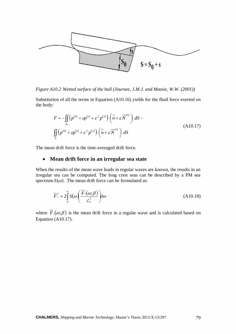
CHALMERS, Shipping and Marine Technology, Master’s Thesis 2013:X-13/297 79
Figure A10.2 Wetted surface of the hull (Journee, J.M.J. and Massie, W.W. (2001))
Substitution of all the terms in Equation (A10.16) yields for the fluid force exerted on
the body:
dSNnppp
dSNnpppF
S
S
)1(2210
)1(2210
0
(A10.17)
The mean drift force is the time-averaged drift force.
Mean drift force in an irregular sea state
When the results of the mean wave loads in regular waves are known, the results in an
irregular sea can be computed. The long crest seas can be described by a PM sea
spectrum )(S . The mean drift force can be formulated as:
d
FSF
a
is
i
2
0
;2 (A10.18)
where ;iF is the mean drift force in a regular wave and is calculated based on
Equation (A10.17).