OPTIMIZATION OF A CO FLOOD DESIGN WASSON FIELD - WEST...

OPTIMIZATION OF A CO2 FLOOD DESIGN

WASSON FIELD - WEST TEXAS

A Thesis

by

MARYLENA GARCIA QUIJADA

Submitted to the Office of Graduate Studies of Texas A&M University

in partial fulfillment of the requirements for the degree of

MASTER OF SCIENCE

August 2005

Major Subject: Petroleum Engineering

OPTIMIZATION OF A CO2 FLOOD DESIGN

WASSON FIELD - WEST TEXAS

A Thesis

by

MARYLENA GARCIA QUIJADA

Submitted to the Office of Graduate Studies of Texas A&M University

in partial fulfillment of the requirements for the degree of

MASTER OF SCIENCE

Approved by: Chair of Committee, David Schechter Committee Members, Walter B. Ayers Wayne M. Ahr Head of Department, Stephen A. Holditch

August 2005

Major Subject: Petroleum Engineering

iii

ABSTRACT

Optimization of a CO2 Flood Design Wasson Field - West Texas. (August 2005)

Marylena Garcia Quijada, B.S., Universidad de Oriente

Chair of Advisory Committee: Dr. David Schechter

The Denver Unit of Wasson Field, located in Gaines and Yoakum Counties in west

Texas, produces oil from the San Andres dolomite at a depth of 5,000 ft. Wasson Field is

part of the Permian Basin and is one of the largest petroleum-producing basins in the

United States.

This research used a modeling approach to optimize the existing carbon dioxide (CO2)

flood in section 48 of the Denver Unit by improving the oil sweep efficiency of miscible

CO2 floods and enhancing the conformance control.

A full compositional simulation model using a detailed geologic characterization was

built to optimize the injection pattern of section 48 of Denver Unit. The model is a

quarter of an inverted nine-spot and covers 20 acres in San Andres Formation of Wasson

Field. The Peng-Robinson equation of state (EOS) was chosen to describe the phase

behavior during the CO2 flooding. An existenting geologic description was used to

construct the simulation grid. Simulation layers represent actual flow units and resemble

the large variation of reservoir properties. A 34-year history match was performed to

validate the model. Several sensitivity runs were made to improve the CO2 sweep

efficiency and increase the oil recovery.

During this study I found that the optimum CO2 injection rate for San Andres Formation

in the section 48 of the Denver Unit is approximately 300 res bbl (762 Mscf/D) of

carbon dioxide. Simulation results also indicate that a water-alternating-gas (WAG) ratio

of 1:1 along with an ultimate CO2 slug of 100% hydrocarbon pore volume (HCPV) will

iv

allow an incremental oil recovery of 18%. The additional recovery increases to 34% if a

polymer is injected as a conformance control agent during the course of the WAG

process at a ratio of 1:1. According to the results, a pattern reconfiguration change from

the typical Denver Unit inverted nine spot to staggered line drive would represent an

incremental oil recovery of 26%.

v

DEDICATION

First to God for so many blessings.

To my beloved husband Sergio, for all his love and encouragement.

To my parents, Juan and Milena, for their unconditional love, caring and support.

vi

ACKNOWLEDGEMENTS Reflecting upon my graduate career, I recognize a great faculty and friends deserving of

my gratitude. They have provided me extraordinary guidance and support. This work is a

reflection of their efforts as much as my own.

I would like to express my sincere gratitude to Dr. David S. Schechter for accepting me

in his research group and assisting and supporting this research. His knowledge,

support, and friendship have made my work possible and enjoyable.

My appreciation also goes to Dr. Walter Ayers and Dr. Wayne Ahr, my committee

members, who were always willing to help me. With their guidance and assistance, I

gained a lot of useful geologic knowledge.

I would like to extend my appreciation to Dr. Erwinsyah Putra for his guidance during

the development of this research.

I am also thankful to Occidental Oil & Gas for providing the field data for this research.

I cannot fully express my gratitude to my friends, Amara Okeke, Rustam Gasimov and

Anar Azimov, for their friendship and for making my days at A&M infinitely more

enjoyable with exceptional grace and good humor. We spent quite a great time together.

vii

TABLE OF CONTENTS

Page

ABSTRACT��................................................................................................ iii

DEDICATION��................................................................................................. v

ACKNOWLEDGEMENTS ................................................................................... vi

TABLE OF CONTENTS....................................................................................... vii

LIST OF FIGURES .................................................................................................. ix

LIST OF TABLES................................................................................................ xiii

CHAPTER

I INTRODUCTION ........................................................................................ 1

1.1 Background ...................................................................................... 1 1.2 Problem Description.......................................................................... 3 1.3 Objectives ......................................................................................... 3

II LITERATURE REVIEW.............................................................................. 4

2.1 CO2 Flooding Mechanisms ............................................................... 4 2.2 Water-Alternating-Gas (WAG) Process ............................................ 5 2.3 WAG Process Classification ............................................................. 7 2.4 Design Parameters for a WAG Process ............................................. 7 2.5 Conformance Control .................................................................... 15

III GEOLOGY REVIEW................................................................................. 17

3.1 Introduction .................................................................................... 17 3.2 Structure ......................................................................................... 20 3.3 Stratigraphy .................................................................................... 22 3.4 Environment of Deposition ............................................................. 26 3.5 Reservoir Geology of the Area ........................................................ 26

IV RESERVOIR PERFORMANCE .................................................................... 28

4.1 Reservoir Basic Data......................................................................... 28 4.2 Reservoir Development (Denver Unit Overview) .............................. 29 4.3 CO2 Flood Development ................................................................... 31

viii

CHAPTER Page

V SIMULATION PARAMETERS AND MODEL ............................................ 37

5.1 Numerical Simulator ......................................................................... 37 5.2 Fluid Properties ................................................................................. 37 5.3 Equation-of-State Characterization.................................................... 38 5.4 Relative Permeability ........................................................................ 48 5.5 Reservoir Model................................................................................ 52 5.6 Initial Conditions............................................................................... 54 5.7 History Match ................................................................................... 54

VI OPTIMIZATION OF MISCIBLE WAG PROCESS..................................... 75

6.1 CO2 Injection Rate Optimization ....................................................... 75 6.2 Optimum Water-Alternating-Gas (WAG) Ratio ................................ 76 6.3 Conformance Control ........................................................................ 78 6.4 Optimum Well Pattern....................................................................... 82

VII CONCLUSIONS .......................................................................................... 85

NOMENCLATURE ............................................................................................... 86

REFERENCES ....................................................................................................... 87

VITA...................................................................................................................... 93

ix

LIST OF FIGURES

FIGURE Page

1.1 Location map of Denver Unit, Wasson San Andres Field��........................ 2

2.1 One-dimensional schematic showing how CO2 becomes miscible with crude oil.....5

2.2 Schematic of the WAG process ..............................................................................5

2.3 Effect of gravity during WAG injection ..................................................................8

2.4 Displacement of oil by water in a stratified reservoir ..............................................9

2.5 Two-phase relative permeability diagram..............................................................11

2.6 Placement of a blocking agent in a high permeability layer ...................................15

3.1 Location of Wasson Field in the Permian Basin.....................................................17

3.2 Generalized stratigraphic column showing Permian Section at the Wasson Field...18

3.3 Structural map of top of San Andres Formation in the Wasson Field. ....................21

3.4 North-south cross section showing the distribution of the depositional facies across Denver Unit in Wasson Field......................................................................23

3.5 Denver Unit type log.............................................................................................25

4.1 Denver Unit production performance ............................................................... 30

4.2 Denver Unit typical well pattern configuration ......................................................32

4.3 Continuous CO2 flood area production performance��.............................. 33

4.4 Continuous CO2 flood area oil cut vs. cumulative oil��............................. 34

4.5 WAG area oil production. ................................................................................ 35

4.6 Cumulative incremental EOR recovery vs. time ��................................... 36

5.1 Preliminary match for the oil FVF ................................................................... 40

x

FIGURE Page

5.2 Preliminary match for the gas deviation factor (Z)............................................ 40

5.3 Preliminary match for the gas FVF .................................................................. 41

5.4 Preliminary match for the oil density (ρo) ........................................................ 41

5.5 Preliminary match for the CO2 swelling factor ................................................. 42

5.6 Preliminary match for the GOR ....................................................................... 42

5.7 Comparison of the predicted and observed values for the GOR ....................... 45

5.8 Comparison of the predicted and observed values for the oil FVF ................... 46

5.9 Comparison of the predicted and observed values for the oil density (ρo) ......... 46

5.10 Comparison of the predicted and observed values for the gas deviation factor (Z) .....................................................................................................47

5.11 Comparison of the predicted and observed values for the gas FVF ................. 47

5.12 Comparison of the predicted and observed values for the CO2 swelling factor 48

5.13 Water and oil relative permeability curves as a function of water saturation ....... 49

5.14 Gas and oil relative permeability curves as a function of gas saturation .............. 50

5.15 Imbibition and secondary drainage water relative permeability .......................... 52

5.16 Simulation grid for Denver Unit section 48 .................................................. 53

5.17 Gas production history match. ........................................................................ 56

5.18 Water production history match...................................................................... 56

5.19 Water cut history match.................................................................................. 57

5.20 Simulated reservoir pressure........................................................................... 57

5.21 Diag-Prod well: Gas production rate history match......................................... 58

5.22 Diag-Prod well: Water production rate history match. .................................... 58

5.23 NS-Prod well: Gas production rate history match. .......................................... 59

xi

FIGURE Page

5.24 NS-Prod well: Water production rate history match........................................ 59

5.25 EW-Prod well: Gas production rate history match. ......................................... 60

5.26 EW-Prod well: Water production rate history match....................................... 60

5.27 Areal view of the oil saturation distribution. Year 0........................................ 62





5.32 Areal view of the oil saturation distribution. Year 10...................................... 64








5.40 E-W cross section showing oil saturation. Year 0 ........................................... 68





5.45 E-W cross section showing oil saturation. Year 10 ......................................... 71

xii

FIGURE Page








6.1 Oil recovery at a WAG ratio of 1:1 as a function of injection rates ................... 75

6.2 Comparison of different WAG ratios in terms of the incremental oil recovery as a function of the CO2 slug size ..................................................................... 77

6.3 Comparison of the residual oil saturation for various WAG ratios after injection of 100% HCPV of CO2 ...................................................................... 77

6.4 East-West cross section view of the simulation model showing the permeability block by the polymer ................................................................... 79

6.5 Injection pressure profile during the viscous water treatment ........................... 80

6.6 Comparison of conformance control treatments as a function of oil production rate........................................................................................................................80

6.7 Comparison of conformance control treatments in terms of the incremental oil recovery as a function of the CO2 slug size....................................................... 81

6.8 (a) Staggered line drive, (b) line drive and (c) nine-spot well patterns ��... ... 82

6.9 Comparison of staggered line drive, line drive and nine-spot well patterns ... ... 83

xiii

LIST OF TABLES

TABLE Page

4.1 Summary of reservoir data��... ................................................................. 29

5.1 Reservoir fluid composition in mole fractions ��... ................................... 38

5.2 P.V.T experimental data................................................................................... 39

5.3 Fluid description for San Andres reservoir fluid ............................................... 48

5.3 Net pay, porosity and permeability distribution in the simulation model........... 53

1

CHAPTER I

2. INTRODUCTION

1.1 Background

The Denver Unit is the largest unit in Wasson Field and is the world�s largest carbon

dioxide enhanced oil recovery (EOR) project. The Denver Unit is located in the southern

edge of North Basin Platform of the Permian Basin in West Texas (Figure 1.1). Primary

depletion drive production began in 1936 with single well production rates greater than

of 1500 STB/D. In 1964, the Denver Unit was formed and a waterflooding was

initiated. Carbon dioxide (CO2) injection began in 1983, when nine inverted nine-spot

patterns were placed on CO2 injection.1

The unit produces from the San Andres Formation, a middle Permian-aged dolomite

located at subsurface depths ranging approximately from 4,800 to 5,200 ft. The Denver

Unit initially contained more than 2 billion bbls of oil in the oil column (OC), which is

the interval of the San Andres hydrocarbon accumulation above the producing oil/water

contact (OWC). The field�s producing oil/water contact (POWC), above which oil is

produced water-free during primary recovery, varies from -1,250 ft to -2,050 ft below

sea level. Above the POWC, petrophysical data generally show that oil occupies the

pore space unsaturated by the reservoir connate water. The San Andres formation

contains more than 650 million bbl of oil in a transition zone (TZ), which is the interval

between the OWC and the true water level, commonly known as the base of zone

(BOZO). The transition zone saturation of 35 to 65% was not effectively recovered by

primary and waterflood primary methods. At Denver Unit, the transition oil has been

proven to be an economical CO2 enhanced oil recovery target.2,3,4

_________________

This thesis follows the style of SPE Reservoir Evaluation and Engineering.

2

N

TEXAS

WASSON SAN ANDRES

FIELD

YO

AK

UM

CO

.

GAINES CO.

DENVERUNIT

TER

RY

CO

.

N

TEXAS TEXAS

WASSON SAN ANDRES

FIELD

YO

AK

UM

CO

.

GAINES CO.

DENVERUNIT

TER

RY

CO

.

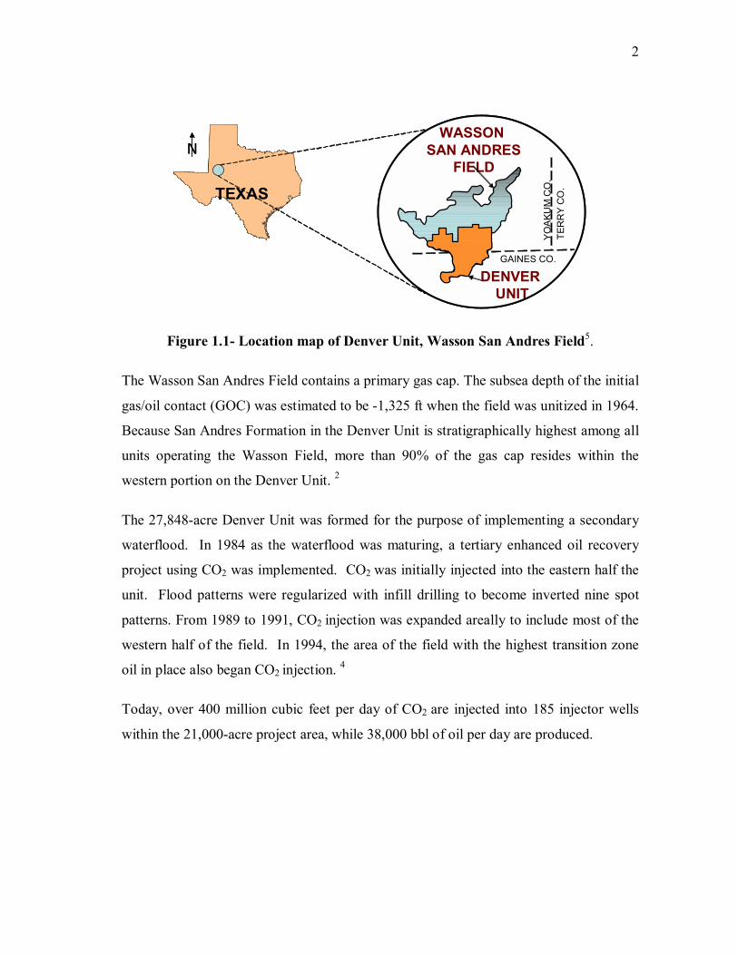
Figure 1.1- Location map of Denver Unit, Wasson San Andres Field5.

The Wasson San Andres Field contains a primary gas cap. The subsea depth of the initial

gas/oil contact (GOC) was estimated to be -1,325 ft when the field was unitized in 1964.

Because San Andres Formation in the Denver Unit is stratigraphically highest among all

units operating the Wasson Field, more than 90% of the gas cap resides within the

western portion on the Denver Unit. 2

The 27,848-acre Denver Unit was formed for the purpose of implementing a secondary

waterflood. In 1984 as the waterflood was maturing, a tertiary enhanced oil recovery

project using CO2 was implemented. CO2 was initially injected into the eastern half the

unit. Flood patterns were regularized with infill drilling to become inverted nine spot

patterns. From 1989 to 1991, CO2 injection was expanded areally to include most of the

western half of the field. In 1994, the area of the field with the highest transition zone

oil in place also began CO2 injection. 4

Today, over 400 million cubic feet per day of CO2 are injected into 185 injector wells

within the 21,000-acre project area, while 38,000 bbl of oil per day are produced.

3

1.2 Problem Description

This research addresses the effects of heterogeneity on the overall sweep efficiency. The

heterogeneity of the formation causes the response to the CO2 injection to vary across

the field, causing poor sweep efficiency and also bypassing a considerable amount of oil.

A reservoir simulation model was used to optimize CO2 injection rates, evaluate

different CO2 injection patterns, determine the optimum WAG ratio, evaluate the use of

a viscous agent in WAG application, and improve conformance control by applying

polymer injection via compositional simulations in section 48 of the Wasson San Andres

Formation.

1.3 Objectives

The main goal of this work was to provide the best methodology to improve the sweep

efficiency of miscible CO2 floods and enhance the conformance control in section 48 in

the San Andres Formation, Wasson Field. The main objectives of this work also

include:

• determining the optimum CO2 injection rates and WAG ratios;

• investigating the effect of conformance control on the ultimate oil recovery;

• studying the effect of pattern changes on the sweep efficiency

4

CHAPTER II

LITERATURE REVIEW

2.1 CO2 Flooding Mechanisms

CO2 flooding processes can be classified as immiscible and miscible, even though CO2

and crude oils are not miscible upon first contact at the reservoir.

Recovery mechanisms in immiscible processes involve reduction in oil viscosity, oil

swelling, and dissolved-gas drive.

In miscible process, CO2 is effective for improving oil recovery for a number of

reasons. In general, CO2 is very soluble in crude oils at reservoir pressures; therefore, it

swells the oil and reduces oil viscosity.6 Miscibility between CO2 and crude oil is

achieved through a multiple-contact miscibility process. Multiple-contact miscibility

starts with dense-phase CO2 and hydrocarbon liquid. The CO2 first condenses into the

oil, making it lighter and often driving methane out ahead of the oil bank. The lighter

components of the oil then vaporize into the CO2-rich phase, making it denser, more like

the oil, and thus more easily soluble in the oil. Mass transfer continues between the CO2

and the oil until the two mixtures become indistinguishable in terms of fluid properties.

Figure 2.1 illustrates the condensing/vaporizing mechanisms for miscibility.7

Because of this mechanism, good recovery may occur at pressures high enough to

achieve miscibility. In general, the high pressures are required to compress CO2 to a

density at which it becomes a good solvent for the lighter hydrocarbons in the crude oil.

This pressure is known as �minimum miscibility pressure� (MMP) and it is the

minimum pressure at which miscibility between CO2 and crude oil can occur.6

5

OilCO2

CO2CO2 vaporizing oil components

CO2 condensing into oil

Original Oil

Miscibility RegionOilCO2CO2

CO2CO2CO2 vaporizing oil componentsCO2 vaporizing oil components



Original Oil

Miscibility RegionMiscibility Region

Figure 2.1- One-dimensional schematic showing how CO2 becomes miscible with

crude oil 7.

2.2 Water-Alternating-Gas (WAG) Process

The WAG process was initially proposed as a method to increase sweep efficiency

during gas injection. In practice the WAG process consists of the injection of water and

gas as alternate slugs by cycles or simultaneously (SWAG), with the objective of

improving the sweep efficiency of waterflooding and miscible or immiscible gas-flood

projects by reducing the impact of viscous fingering.8 The WAG process is

schematically shown in Figure 2.2.

OilMisciblezoneCO2WaterCO2Water OilMisciblezoneCO2WaterCO2Water Misciblezone

MisciblezoneCO2WaterCO2Water CO2CO2WaterCO2Water WaterWaterCO2CO2WaterWater

Figure 2.2- Schematic of the WAG process (Kinder Morgan Co.).

6

During a WAG process, the combination of higher microscopic displacement efficiency

of gas with better macroscopic sweep efficiency of water helps significantly increase the

incremental production over a plain waterflood.

WAG process has had a wide acceptance in field operations in the United States. A

wide variety of gases have been employed for a wide range of reservoir characteristics in

the miscible mode; however, CO2 and hydrocarbon gases represent approximately 90%

of the injectant gases used.7

The mobility ratio between injected gas and the displaced oil bank by CO2 and other

miscible gas displacement processes is typically very unfavorable because of the

relatively low viscosity of the injected phase. A very unfavorable mobility ratio results

in viscous fingering and reduced sweep efficiency. The WAG process is an injection

technique developed to overcome this problem by injecting specified volumes, or slugs,

of water and gas alternatively. As results of this process, the mobility of the injected gas

alternating with water is less than that of the injected gas alone, and thus the mobility

ratio of the process is improved.

In WAG injection, water/gas injection ratios have ranged from 0.5 to 4.0 volumes of

water per volume of gas at reservoir conditions. The sizes of the alternate slugs range

from 0.1% to 2% of the pore volume (PV).9 Total or cumulative slug sizes of CO2 in

reported field projects typically have been 15% to 30% of the hydrocarbon pore volume

(HCPV), although smaller and larger slugs have been reported. 10

The main factors affecting the WAG injection process are the reservoir heterogeneity

(stratification and anisotropy), rock wettability, fluid properties, miscibility conditions,

gas trapped, injection technique and WAG parameters such as slug size, WAG ratio and

injection rate. 11

7

2.3 WAG Process Classification Although Claudle and Dyes8 suggested simultaneous injection of oil and gas to improve

mobility control, the field reviews show that they are usually injected separately.12 The

main reason for this injection pattern is the better injectivity when only one fluid is

injected.

WAG processes have been classified into four types: miscible, immiscible, hybrid and

others on the basis of injection pressures and method of injection. Many reservoirs

specific processes have been patented and are generally grouped under the �other� WAG

classification.12

A number of different WAG schemes are used to optimize recovery. Unocal patented a

process called �Hybrid-WAG� in which a large fraction of the pore volume of CO2 is

injected continuously, followed by the remaining fraction divided into 1:1 WAG ratios.13

Shell developed a similar process called DUWAG14 (Denver Unit WAG) by comparing

continuous injection and WAG processes

2.4 Design Parameters for a WAG Process

Miscible gas injection has been implemented successfully in a number of fields around

the world.12 In principal the WAG process combines the benefits of miscible gas

injection and waterflooding by injecting the two fluids simultaneously or alternatively.

Miscible gas injection has excellent microscopic sweep efficiency but poor macroscopic

sweep efficiency due to viscous fingering and gravity override. Furthermore it is

expensive to implement in contrast to waterflooding, which is relatively cheap and is

less subject to gravity segregation.

For this reason, it is very important to develop various CO2 flood designs to determine

the optimum near-term cash flow, overall project economics, and oil recoveries. The

major design issues for a WAG injection process are reservoir characteristic and

8

heterogeneity, rock and fluids characteristics, injection pattern, WAG ratio, injection

rate, ultimate CO2 slug size.

2.4.1 Reservoir Heterogeneity and Stratification

Reservoir and heterogeneity stratification have a strong influence on the water/gas

displacement process.11 The degree of vertical reservoir heterogeneity can affect the

CO2 performance. Reservoirs with higher vertical permeability are influenced by cross-

flow perpendicular to the bulk flow direction.15 Cross-flow may increase the vertical

sweep, but generally the gravity segregation and decreased flood velocity in the reservoir

reduce the oil recovery (Figure 2.3). As CO2 flows preferentially toward the top portion

of thick, high permeability zone, injected water may flow preferentially toward the lower

portion of the zone.

CO2 and Oil

Water and Oil

CO2 Injection Cycle

Water Injection Cycle

Water and Oil

CO2 and Oil

CO2 and Oil

Water and Oil

CO2 Injection Cycle

Water Injection Cycle

Water and Oil

CO2 and Oil

Figure 2.3- Effect of gravity during WAG injection 7.

9

Reservoir heterogeneity controls the injection and sweep patterns in the flood. Reservoir

simulation studies16 for various vertical to horizontal permeability (kv/kh) ratios suggest

that higher ratios adversely affect oil recovery in WAG process.

Other studies17 have reported that the vertical conformance of WAG displacements is

strongly influenced by conformance between zones. In a non communicating layered

system, vertical distribution of CO2 is dominated by permeability contrasts. Flow into

each layer is essentially proportional to the fractional permeability of the overall system

[(average permeability x layer thickness (kh)] and is independent of WAG ratio,

although the tendency for CO2 to enter the high permeability zone with increasing WAG

ratio cannot be avoided. Due to the cyclic nature of the WAG, the most permeable layer

has the highest fluid contribution, but as water is injected it quickly displaces the highly

mobile CO2 and all the layers attain an effective mobility nearly equal to the initial

value.

In highly stratified reservoirs, the higher permeability layer(s) always respond first,

resulting in an early breakthrough and poor sweep efficiency. See Figure 2.4. For these

heterogeneous reservoirs, a WAG process would reduce the mobility in the high

permeability layer, resulting in a larger amount of the CO2 contacting the crude oil in

that particular layer.

High K

Low K Oil

Oil

Water Oil

Injector Producer

High K

Low K Oil

Oil

Water Oil

Injector Producer

Figure 2.4- Displacement of oil by water in a stratified reservoir.

10

Alternate CO2/water injection is more sensitive to changes in reservoir properties, such

as different permeabilities, than is waterflooding. Continuous CO2 injection is even

more sensitive to reservoir properties because there is no injected water to help control

volume sweep by slowing down the movement of CO2.

High-permeability layers, directional permeability trends, and natural fractures all cause

sweep problems. If a reservoir is naturally fractured to the extent that fractures have

adversely affected waterflood sweep, a CO2 flood using the same pattern is very likely to

be unsuccessful.

2.4.2 Relative Permeabilities

Relative permeability is an important petrophysical parameter, as well as a critical input

parameter, in predictive simulation of miscible floods. However, relative permeability is

a lumping parameter that includes the effects of wetting characteristics, heterogeneity of

reservoir fluids and rock and fluid saturations.18

During a typical CO2 flood that includes injecting water alternately with CO2 to remedy

areal and vertical sweep problems, saturation changes during each injection period.7

These changes in saturation also result in changes in the water relative permeability.

Among one of the most common problems associated with relative-permeability changes

during alternate water/CO2 floods are injectivity losses.18 Water injectivity undergoes

significant changes after the first cycle of injected CO2. These changes are related to the

effect that CO2 has on the relative permeability of the water. A quantitative

understanding of the relative permeability curves is important because is an input to

reservoir simulators to forecast the CO2 flood performance.7

Simulation sensitivities19 have shown that a sharp injectivity reduction at the start of the

water cycle can be associated with relative permeability reduction near the well that can

gradually experience an increasing injectivity trend throughout the rest of the cycle.

11

This behavior is suggested to be caused by two-phase flow of gas and water initially near

the well; as the cycle proceeds, the saturations and the relative permeabilities change. 18

Laboratory floods attempting to emulate CO2 flood20 experienced appreciable water

relative permeability reductions after CO2 injection. In addition, data have shown

significant hysteresis effects in the water relative permeability between the drainage and

imbibition curves. Irreducible water saturations after drainage cycles were 15 to 20%

higher than the initial connate water saturation.18

Hysteresis refers to the directional saturation phenomena exhibited by many relative

permeability and capillary-pressure curves when a given fluid phase saturation is

increased or decreased.21 This phenomenon is illustrated in Figure 2.5.

Water Saturation, fraction0.2 0.3 0.4 0.5 0.6 0.7 0.8

Oil

Water

Water(hysteresis)

1.0

0.1

0.01

0.001

Maximum Krwfor waterflood

Rel

ativ

e Pe

rmea

bilit

y, fr

actio

n

Water Saturation, fraction0.2 0.3 0.4 0.5 0.6 0.7 0.8

Oil

Water

Water(hysteresis)

1.0

0.1

0.01

0.001

Maximum Krwfor waterflood

Rel

ativ

e Pe

rmea

bilit

y, fr

actio

n

Figure 2.5- Two-phase relative permeability diagram7.

The figure represents a test of bidirectional water/oil relative permeability that depicts

the water relative permeability and water injectivity. The relative permeability of the oil

is 1.0 at connate water saturation and declines as a waterflood is performed until residual

12

oil saturation is reached. Simultaneously, the relative permeability of water increases

until a maximum value is reached.

Then, oil is injected until water ceases to flow. For an oil-wet reservoir, oil can flow

back through the same pores that it previously vacated, and the oil relative permeability

can increase along the same path. The water relative permeability, however, shows

hysteresis because the drainage (decreasing oil and increasing water saturation) and

imbibition (increasing oil and decreasing water saturation) curves do not follow the same

path. As a result, the new minimum value of irreducible water saturation does not go

back to the original connate-water saturation.

The result of water-permeability hysteresis in an oil-wet reservoir is that water

injectivity can be severely reduced. In addition, oil relative permeability can not return

to 1.0 because the increased residual water saturation reduces the maximum oil

saturation possible, consequently reducing the tertiary oil rate.7

2.4.3 Injection Patterns

Well injection patterns and well spacing have a great impact on the sweep efficiency in a

CO2 flood. Additionally, well spacing is a strong indicator of the average reservoir

pressure (as the ratio of injector to producers increases, so does the average reservoir

pressure). 7

The most popular pattern injections in the field are the five-spot pattern and the inverted

nine-spot patters. The 5-spot pattern gained high popularity in field operations during

CO2 floods because its well spacing makes it attain better flood- front control and helps

to maintain higher average reservoir pressure.7 The inverted nine-spot pattern was also

very common in the early years of many CO2 floods in west Texas.4,22

Regardless of the type of pattern used for a CO2 flood, it is very important and critical to

prevent major volumetric sweep problems under the operation. Problems with low

13

reservoir pressure and poor sweep efficiency during a waterflooding will definitely get

worse during a CO2 flooding.7

In general, fields with high well spacing (greater than 80 acres) are likely to have a poor

CO2 flooding incremental recovery due to low sweep efficiency. Those fields would

likely require a significant additional capital investment in infill wells to improve the

production and the economic attractiveness of CO2 flooding development.4, 23

2.4.4 WAG Ratios

WAG ratio is the ratio of injected water to CO2. WAG ratios may be expressed in terms

of reservoir injection (i.e., barrels of water injected at reservoir conditions) or in terms of

duration (i.e., the time over which injection takes place).7 The WAG ratio is controlled

by the gas availability as well as the wetting state of the reservoir rock.16

Injecting water with miscible gas reduces the instability of the gas/oil displacement

process that results from relative permeability effects, thus improving the overall sweep

efficiency. It also improves the economics by reducing the volume of gas that needs to

be injected into the reservoir.

An optimum WAG ratio is a major parameter design that has a significant effect on both

operation and economics of a CO2 flood. An approach to maximize the net present

value of a CO2 flood 24 suggests that WAG ratio should be increased gradually after the

optimum gas production is reached through the life of the flood. The gradual increase of

injected water (a decrease in the WAG ratio) results in increased mobility control and a

constant produced gas profile.

Laboratory studies16 on WAG ratios showed that tertiary CO2 floods have maximum

recoveries at a WAG ratio of about 1:1 in floods dominated by viscous fingering

whereas 0:1 WAG ratio (continuous gas injection) showed optimum recovery in floods

dominated by gravity tonguing. Hence, continuous gas injection is recommended for

14

secondary as well as tertiary floods in water-wet rocks, whereas 1:1 WAG is

recommended for partially oil-wet rocks.

In practice all patterns may start at the same WAG ratio. Later, as the CO2 production

increases due to poor volumetric sweep efficiency, the WAG ratio is usually increased

on a pattern-by-pattern basis starting with the highest GOR patterns. 7

2.4.5 Slug Size

Slug size refers to the cumulative of CO2 injected during a CO2 flood. The slug volume

is usually expressed as a percentage of the hydrocarbon pore volume (%HCPV).7

Selecting an optimum CO2 slug size is critical in a proper design of a hydrocarbon

miscible flood.25 Generally, the more CO2 injected, the greater the incremental oil

recovery. However, a large CO2 slug size diminishes the return of the project. The

larger the CO2 bank size, the greater the ultimate recovery, but the increment gets

smaller and smaller.26

Economic sensitivities must be performed to determine the optimum CO2 slug size. The

optimum CO2 slug size for a particular project will depend upon economic factors such

as crude price, CO2 cost, and the amount and timing of the incremental recovery. The

economic optimization process is carried out by systematically repeating simulation runs

until optimum design parameters are achieved.27 Total slugs of CO2 equal to about 20 to

50% HCPV have been used in different projects in U.S.A.28

The ultimate CO2 slug size can be determined after the start of project, when more

information is known about future price of oil and production response of the reservoir.

The optimum CO2 bank size should be determined on an individual pattern basis rather

than on a total project evaluation.26

15

2.5 Conformance Control

Conformance is a measure of where injected fluids (water or CO2) are entering the pay

zone. Ideally, injected fluids enter the formations only at pay zones and spread out

evenly across these zones to avoid early breakthrough.7

When a WAG has failed to control sweep, other techniques such as surfactant foams, gel

polymers and conventional plugging methods can be used to improve the sweep

efficiency of the injection process.7

The objective of gel treatments and similar blocking-agent treatments is to reduce

channeling through fractures or high-permeability zones without significantly damaging

hydrocarbon productivity. The idea is to achieve a permeability reduction in high

permeability layers, while minimizing gel penetration and permeability reduction in less-

permeable, hydrocarbon-productive zones. This objective can be met by mechanically

isolating zones during the gel-placement process, so that gel injection occurs only in the

high-permeability zones.28 See figure 2.6.

Low K

High KBlocking Agent

Low K

High KBlocking Agent

Figure 2.6- Placement of a blocking agent in a high permeability layer.

If analogous flood suggests that premature water/CO2 breakthrough will be a problem, or

representative core data indicate that the reservoir will not flood uniformly, polymers or

blocking agent treatments should be carried out to avoid sweep efficiency problems.

Expected results are more oil produced faster and at lower gas/oil ratios.

16

The initial step in treatment design is selecting a process appropriate for the reservoir

problem. Choices to be made include near-wellbore versus deep gel treatments, type of

polymer, crosslinking agent, and crosslinking process. On-site and laboratory testing by

service companies with actual treating/reservoir fluids assists in chemical selection and

treatment design.29

A critical step is the calculation of the treatment volume and the prediction of variation

in polymer composition. Diverse tools, such as production/injection histories, well logs,

surveys, workover history and personal knowledge of the formation and geographical

area are critical for prediction of treatment volume. It is impossible to calculate

treatment volume exactly, but estimation within reasonable limits is possible. That is

why it is essential that injection rate and pressure be continuously monitored during

treatment and appropriate changes made to optimize treatment. The polymer solution

should be injected until parting pressure is approached while injecting, the injected slug

is produced at a peripheral producer, or the maximum design size is achieved. In most

cases, parting pressure is the limiting factor for treatment size.30

17

CHAPTER III

2. GEOLOGY REVIEW

3.1 Introduction

Wasson Field is situated near the central part of the Staked plain in Yoakum and Gaines

Counties on the southeastern margin of the northwest shelf of the North Basin Platform

of the Permian Basin, west Texas (Figures 1.1 and 3.1). It occupies a triangular area 15

miles long and 14 miles wide, containing approximately 55,000 acres or 86 square miles,

and includes only a few dry holes.31

EasternShelf

Wasson Field

GuadalupeMountains

Northwest ShelfTe

xas

New

Mex

ico

DelawareShelf

Miles

0 30Central Basin Platform

Denver UnitEastern

Shelf

Wasson Field

GuadalupeMountains

Northwest ShelfTe

xas

New

Mex

ico

DelawareShelf

Miles


Denver Unit

Wasson Field

GuadalupeMountains

Northwest ShelfTe

xas

New

Mex

ico

DelawareShelf

Miles

0 30

MilesMiles


Denver Unit

Figure 3.1- Location of Wasson Field in the Permian Basin32.

18

Geologically, the field lies on the extended axis of the Central Basin platform, but

appears to be separated from it by a trough in northern Gaines County. The combined

effect of the structural elements gives the appearance of a terraced platform tilted

northeastward by post-Permian movement. 32

Wasson Field produces oil from the Permian San Andres dolomite. The stratigraphy of

San Andres Formation is typical of west Texas. Massive and porous dolomites with few

clastics grade basinward into sections of interbedded dolomite, anhydrite and minor

limestones. The San Andres Formation is overlain by the Grayburg formation which is

not productive in the Wasson field.32, 33, 34 Figure 3.2 is a generalized stratigraphic

column showing Permian formations present at Wasson Field. Within this section,

production is predominately from dolomites of the Guadalupian-aged Andres

Formations.

PERIOD EPOCH

PaddockBlinebryTubbDrinkard

Wolf-campian

FORMATION

Glorieta

Dewey LakeRustlerSalado

YesoAbo

Wolfcamp

TansillYates

Seven RiversQueen

GrayburgSan Andres

Per

mia

n

Ochoan

Gua

dalu

pian

Leon

ardi

an

Figure 3.2- Generalized stratigraphic column showing Permian Section at the

Wasson Field. Productive interval San Andres Formation is shaded.34

19

Wasson field is a combination of structural/stratigraphic trap controlled by a

combination of an extensive dolomitization and anhydrite plugging.34 The structure is

an anticline capped by dense dolomite and underlain by an essentially inactive aquifer.

Structure and stratigraphy in San Andres Formation appear to have controlled the

permeability, porosity, and the accumulation of fluids.32 San Andres Formation at

Wasson Field presents vertical and lateral variations with respect to petrophysical

properties that make the formation highly heterogeneous. The stratigraphic component

of vertical heterogeneity is apparent in the cyclic character of the San Andres Formation

caused by high-frequency changes in relative sea level during San Andres deposition.

Vertical heterogeneity within the San Andres is also strongly affected by post-

depositional and diagenetic processes.34, 35

Lateral variability in porosity and permeability patterns is a function of both depositional

and post-depositional processes. Depositional causes such as lateral carbonate texture

variation and variations in water depth produced by paleotopography and by relative

facies positions on the ramp contribute to lateral heterogeneity within the San Andres

Formation.36, 37 Post depositional controls on lateral heterogeneity include spatially

varying degrees of dolomitization, anhydritic replacement of dolomite crystals,

anhydritic filling of void space and moldic porosity development. In addition to these

post-depositional effects, faults, fractures and associated diagenesis quite likely

contribute to lateral heterogeneity within the Permian carbonate section.33, 37

Analyses of core and log data indicate the presence of extensive dolomitization, moldic

and vuggy porosity development, and anhydrite emplacement.37 Six pore types have

been identified in San Andres Formation related to both depositional and diagenetic

changes. The pores types include intercrystal, vug, moldic, intracrystal, fracture, and

intraparticle.33 These processes act at a variety of scales and impose a substantial

contribution to vertical heterogeneity within the reservoir.

20

3.2 Structure

Wasson Field resulted from structural drape over the buried Abo trend on the southeast

and the stratigraphic facies changes to the northwest.35

San Andres Formation combines stratigraphic trapping of hydrocarbons from porosity

pinch-outs and anhydrite plugging with subtle structural nosing and changes in dip.

These structural elements on both local and regional scale have an important influence in

the location of hydrocarbons in the San Andres Formation. 34

The present structural attitude of the beds is the result of the cumulative, gentle pre-

Tertiary folding plus thel eastward tilting of the region during the Tertiary. The present

structure is best shown by contouring the �solid lime� or top of the San Andres

Formation. It is compound, consisting of two dominant lines of folding: one trending N

30° E, along the east edge of the field; the other N 65° W, along the southwest edge.32

San Andres Formation has a triangular shape on an areal perspective (Figure 3.3). The

structure is bordered by relatively steep flanks on the southeast and southwest which dip

approximately 3°. The dip in the north flank of the formation is less than 100 ft/mile.

The southeastern limit of the field closely parallels the edge of the North Basin Platform,

which is the shelf margin of the underlying Lower Clearfork and Wichita

Formations.31, 32

21

-150

0-1

400

-130

0

-120

0-1

300

-110

0

-140

0

-150

0

-1400

-140

0

-130

0

1 m

iDe

nver

Un

it

-150

0-1

400

-130

0

-120

0-1

300

-110

0

-140

0

-150

0

-1400

-140

0

-130

0

1 m

i1

miD

en

ver

Un

it

Figu

re 3

.3- S

truc

tura

l map

of t

op o

f San

And

res F

orm

atio

n in

the

Was

son

Fiel

d2 .

22

3.3 Stratigraphy

San Andres Formation is Middle Permian (Guadalupian) in age and in the Wasson Field

consists in 1,300 feet of dolomite.31 It is located between the evaporitic dolomites of

Grayburg Formation, which is not productive in the Wasson area, and the sandy

anhydritic dolomites of Glorieta Formation. The reservoirs are located in the lower part

of the San Andres and are capped by nearly 400 ft of a dense nonporous dolomite.31,35

The Wasson San Andres field is a classic example of a carbonate reservoir located on a

regressive carbonate shelf platform. Core examination reveals a classic example of a

shoaling-upward sequence where the original sedimentary environments clearly

influenced the development and distribution of porosity.31

The San Andres Formation in the Northwest Shelf represents a regressive series of cyclic

deposits that prograded southward across a broad, low relief, shallow-water shelf. San

Andres Formation consists of interbedded dolomites, anhydrites, and minor limestones.

The lower part of San Andres is up to 800 ft thick and is a large-scale shoaling

depositional cycle composed, from bottom to top, of open marine shelf deposits;

restricted-marine, subtidal dolostones that from the reservoir facies; intertidal and

supratidal dolostones, and salina and sabkha anhydrites. 34

The San Andres Formation is characterized by a basinward progradational shift in facies;

this overall shift is interrupted by several transgressions, which result in the cyclical

nature of the carbonate section. Gradual return to the regressive conditions resulted in

the deposition of intertidal to supratidal nonporous dolomite interbedded with anhydrite

that caps the lower San Andres productive interval.35

The principal reservoir rocks are a mixture of two end-member rock types: pelletal

packstones and moldic (skeletal) wackestones. The pelletal packstones are usually well

burrowed, contain varying amounts of skeletal debris, and are usually less than 10 ft

thick. The moldic wackestones are slightly burrowed and occur as patchy accumulations.

23

Fluid-flow properties reflect the relative proportions of pelletal packstone and moldic

wackestone. The pelletal packstones have abundant interparticle porosity with varying

amounts of moldic pores; their porosity commonly ranges between 15 and 20%, but

locacally is as high as 25%. Permeability is usually between 10 and 50 md, but very

locally exceeds 100 md. The most abundant pore type in the wackestones is moldic. This

rock type has a permeability of less than 1 md, although moldic porosity may range as

high as 10%.33

The San Andres Formation has been stratigraphically divided into two major intervals

known as �First Porosity� and �Main Pay.� The Main Pay, which is the lower interval,

consists of dolomitized open marine packstones and wackstones and exhibits better

quality rock than the First Porosity interval. The First Porosity interval possesses poor-

quality reservoir rock and was deposited in shallower-water, restricted marine and

intertidal environment. The First Porosity has finer crystalline matrix and is less

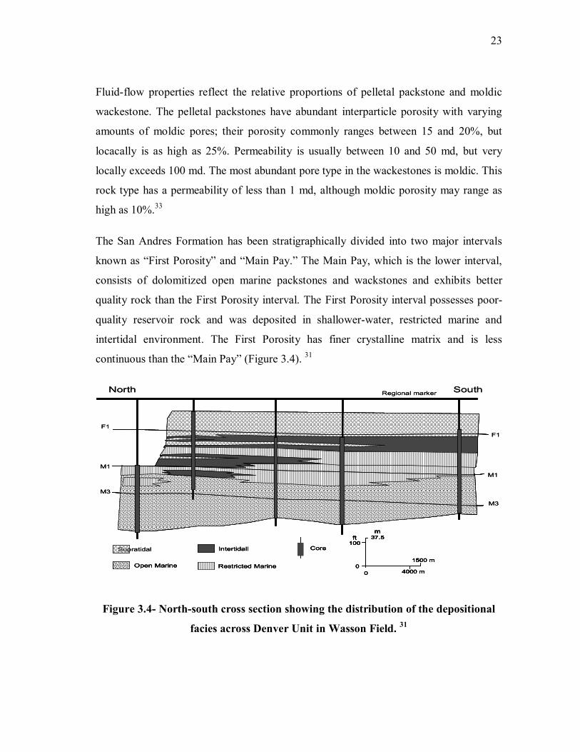
continuous than the �Main Pay� (Figure 3.4). 31

Regional marker SouthNorth

F1

M1

M3

F1

M1

M3

Supratidal

Open Marine

Intertidall

Restricted Marine

Core

00

10037.5ftm

1500 m

4000 m

Regional marker SouthNorth

F1

M1

M3

F1

M1

M3

Supratidal

Open MarineOpen Marine

IntertidallIntertidall

Restricted MarineRestricted Marine

CoreCore

00

10037.5ftm

1500 m

4000 m0

0

10037.5ftm

1500 m

4000 m0

0

10037.5ftm

1500 m

4000 m

Figure 3.4- North-south cross section showing the distribution of the depositional

facies across Denver Unit in Wasson Field. 31

24

Main Pay subtidal pelletal packstones in the Denver Unit have porosity of 15 to 20% and

permeability from 10 to 50 md, whereas the Main Pay moldic wackestones have porosity

as high as 10 percent but permeability less than 1 md.31

On the basis of the gamma ray and sonic logs, the first porosity was divided into five

intervals (F1 through F5), and the main pay was divided into six zones (M1 through

M6). These zones can be recognized throughout the Denver Unit. Figure 3.5 is a type

log showing the present divisions of the San Andres Formation in the Denver Unit.2

Simulation layers were built on the basis of the actual stratigraphical division of the San

Andres Formation. This representation of the flow units would honor the heterogeneity

and zonation of the formation.

In the simulation model, additional divisions of the existing geologic zones were

necessary to represent large variations in porosities and permeabilities within the

geologic zones. For example, the �M1� interval was subdivided into four layers because

has high permeability contrast. Similarly, the�M3� interval has also divided into three

layers since the upper part of interval presents a high permeability value in comparison

with the rest of the zone. See Figure 3.5.

25

GR Porosity Perm

F3F4F5M1

M2M3

M4

M5

F1

F2

M6OWC

GOC

F Zone�First Porosity�

0 100 0.3 0 0.1 100Feet

4800

4900

5000

5100

5200

5300

M Zone�Main Pay�

OilColumn

TransitionZone

Base Of

Zone

GR Porosity Perm

F3F4F5M1

M2M3

M4

M5

F1

F2

M6

F3F4F5M1

M2M3

M4

M5

F1

F2

M6OWC

GOC

F Zone�First Porosity�

0 100 0.3 0 0.1 100Feet

4800

4900

5000

5100

5200

5300

M Zone�Main Pay�

OilColumn

TransitionZone

Base Of

Zone

Courtesy of Occidental Oil and Gas

Figure 3.5- Denver Unit type log.

26

3.4 Environment of Deposition

Deposition occurred in a shallow marine shelf environment. Moldic wackestones

represent the original sediment. Pelletal packstones are probably the remains of fecal

pellets produced by organisms which burrowed through the muddy sediment. When this

burrowing was very intense, a sediment consisting entirely of pellets was produced as

organisms reworked sediment. When burrowing was less prevalent, pellets were

restricted to well-defined burrows cutting through wackestone sediment. Both

dolomitizing and anhydrite precipitating fluids were probably derived from overlying,

supratidal sediments deposited after the open marine reservoir rocks. The original

sediment was composed entirely of calcite and aragonite with no associated dolomite or

gypsum.33

3.5 Reservoir Geology of the Area

Cores analyses have revealed that the Main Pay interval presents three rock types: a

pelletal dolomite packstone with interparticle and intercrystal porosity (pelletal

packstone); a fossiliferous dolomite wackestone with moldic porosity (moldic

wackestone); and a fossiliferous dolomite packstone with moldic and interparticle

porosity (moldic packstone).33

The pelletal packstone rocks occur both as homogeneous units and in burrows and

irregular patches in the wackestones. They have excellent reservoir rock properties;

permeability can be as high as 152 md and interparticle porosity is up to 24.3%. 33

In the wackestone rocks, molds and vugs are the dominant pore types, ranging in size up

to 6 mm. Within the rock, molds are not in contact with other; core observation has

revealed that the molds are isolated in the rock by a relatively tight matrix. This isolated

moldic porosity negatively affects the reservoir properties of the rock. Permeability is

less than 1 md, even though moldic porosity may range as high as 10%. 33

27

The moldic packstone rock is medium crystalline, with more moldic than intercrystal

porosity and light brown. Due to the connection of the moldic pores through interparticle

pores, these rocks exhibit higher permeabilities and lower residual oil saturations than

any other rock types in the area.33

Average reservoir porosity and permeability are 12% and 5 md, respectively. Lateral

reservoir continuity at the pattern scale (injector to producer distance averages

approximately 1,000 ft) is generally considered good.

28

CHAPTER IV

3. RESERVOIR PERFORMANCE

4.1 Reservoir Basic Data

The Denver Unit is the largest unit in Wasson Field. The unit produces oil from the San

Andres Formation, a Middle Permian dolomite located at subsea depths ranging from

approximately -1,250 to -2,050 ft.

The Denver Unit initially contained more than 2 billion bbl of oil in the oil column,

which is the interval of the San Andres hydrocarbon accumulation above the producing

oil/water contact (OWC). In addition, the San Andres Formation contains more than 650

million bbl of oil in a transition zone (sometimes referred to as a paleo residual oil zone).

The gross oil pay thickness of the San Andres Formation varies from 200 to 500 ft. The

formation contains a primary gas cap. The subsea depth of the initial gas/oil contact

(GOC) was estimated to be -1,325 feet. Because the San Andres Formation in the

Denver Unit is stratigraphically highest among all units operating the Wasson Field,

more than 90% of the gas cap resides within the western portion of the Denver Unit. The

presence of the gas cap has had a great impact on the CO2 flood performance. The

formation is underlain by an essentially inactive aquifer. Solution drive has been the

primary producing mechanism.2,3

Table 4.1 summarizes basic reservoir and fluid data.

29

Table 4.1- Summary of reservoir data

Reservoir Characteristics Values Producing area 25,505 acres Formation Permian San Andres Dolomite Average Depth 5,200 ft Gas-oil Contact -1,325 ft Average Permeability 5 md Average Porosity 12% Average net oil pay thickness 137 ft Oil Gravity 33° API Reservoir Temperature 105°F Primary production mechanism Solution-gas drive Secondary production mechanism Waterflood Tertiary production mechanism CO2 miscible Original reservoir pressure 1,805 psi Bubble point pressure 1,805 psi Average pressure at start of secondary recovery ±800 / ±1100 psi Target reservoir pressure for CO2 2,200 psi Initial FVF (Formation Volume Factor) 1.312 res bbl/bbl Solution GOR at original pressure 420 res bbl/bbl Solution GOR at start of secondary recovery original pressure

1,060 scf/bbl

Oil viscosity at 60° F and 1100 psi 1.18 cp Minimum miscibility pressure 1,300 psi

4.2 Reservoir Development (Denver Unit Overview)

Wasson Field was discovered in 1936. Primary depletion drive production began in

1936 with single-well production rates in excess of 1,500 barrels of oil being common.1

By the mid 1940s, the field was largely developed on a 40-acre well spacing. The 27,848

acre Denver Unit, covering the southern portion of Wasson Field , was formed in 1964

for the purpose of implementing a secondary flood. In 1966, supplemental recovery

30

operations were initiated and waterflood operations began. Peak secondary oil

production of 37,100 BOPD occurred in 1975.3

In 1984 as the waterflood was maturing, a tertiary enhanced oil recovery project using

carbon dioxide was implemented. The Denver Unit CO2 flood, ranks among the largest

EOR projects currently operating in the United States. Historical waterflood and tertiary

performance of Denver Unit are shown in Figure 4.1.

CO2 was initially injected only in the eastern half of the unit. Floods were regularized

with infill drilling to become inverted nine-spot patterns. From 1989 to 1991, CO2

injection was expanded aerially to include most of the western half of the field. In 1994,

the area of the field with the highest transition zone oil in place, commonly known as the

TZ sweet spot, also began CO2 injection. Infill drilling and pattern reconfiguration

development were initiated in 1995 and continued to the present time.4

0

40000

80000

120000

160000

200000

1964 1966 1969 1972 1975 1978 1981 1984 1987 1990 1993 1996 1999 2002 2005Year

Rat

es (B

OPD

, BW

PD, M

CFD

)

Oil Production Gas Production Water Production

Waterfllooding

CO2 Flood

0

40000

80000

120000

160000

200000

1964 1966 1969 1972 1975 1978 1981 1984 1987 1990 1993 1996 1999 2002 2005Year

Rat

es (B

OPD

, BW

PD, M

CFD

)

Oil Production Gas Production Water Production

Waterfllooding

CO2 Flood

Figure 4.1- Denver Unit production performance.

31

4.3 CO2 Flood Development

Following the success of the Denver Unit waterflood and the high waterflood residual oil

saturations (approximately 40%), EOR process studies and laboratory experiments

indicated that miscible CO2 injection could result in significant EOR potential in this

reservoir.

A CO2 pilot was initiated in 1978, and analysis of this pilot confirmed that adequate CO2

injection followed by water injection could be attained. The pilot also quantified the

reduction in oil saturation resulting from CO2 injection at waterflood residual oil

saturation.

Following extensive coring and a brine preflood to establish the baseline oil saturations

and a uniform reservoir pressure, CO2 was injected at miscible conditions. The cored

interval extended 50 ft below the estimated original oil/water contact, allowing the

evaluation of CO2 floodable oil saturation in the transition zone.38

Throughout the CO2 and brine post-flood phases of the pilot, logging observation wells

continuously monitored changes in oil saturation attributable to the CO2 contacting and

swelling, and displacement of the remaining oil. Post-flood cores confirmed the

desaturation of oil interpreted from logging runs.18, 39, 40

In preparation for the CO2 flood, the random waterflood pattern was converted into a

nine-spot pattern (Figure 4.2). In addition, reservoir pressure was reduced from 3,200

psi to 2,200 psi in order to improve the volumetric efficiency of the CO2 (and yet

maintain reservoir pressures above the MMP of 1300 psi).39

Miscible carbon dioxide injection began in 1984 when nine-spot patterns were placed on

CO2 injection. Production response to CO2 has been impressive, with over half of the

current daily oil production attributable to CO2 injection. In fact, oil production has

substantially exceeded original project performance predictions.38 Historical waterflood

and tertiary performance of Denver Unit are shown in Figure 4.1.

32

Injection Well

Producer Well

Injection Well

Producer Well

Injection Well

Producer Well

Figure 4.2- Denver Unit typical well pattern configuration.

To determine the best injection strategy for the Denver Unit, two simultaneous CO2

floods were carried out in different areas of the reservoir. One area was operated under a

continuous CO2 injection flood, whereas in the other area, a Water-Alternating-Gas

(WAG) CO2 injection was implemented.

In both cases, an injection of a 40% hydrocarbon pore volume (HCPV) CO2 slug was

planned, followed by water injection until the economic limit was reached. The WAG

operating scheme was used for mobility control to maximize flood profitability through

improved sweep efficiency and to minimize the volume of the more expensive CO2

required.

The early production performance of the continuous CO2 injection flood area was very

encouraging. Oil production response was observed soon after injection began (Figure

4.3) and the oil cut rose from a low of 14% to 31%. CO2 response can be clearly seen on

a plot of oil cut vs. cumulative production (Figure 4.4).

Following a short period of CO2 injection, the oil cut deviated markedly upward from

what would have been expected under continued waterflood conditions. Another

indicator of EOR response in the early years of the CO2 flood was the rising GOR as the

33

flood progressed. This increase in the GOR was a consequence of the stripping of the

lighter hydrocarbon components out of the remaining oil as CO2 contacts oil in the

reservoir.

Wells located east to west of pattern injection experienced an earlier EOR response,

whereas wells located north to south of CO2 injectors, or diagonally to pattern injectors,

responded more slowly to CO2 injection. This oil response characteristic of the

continuous area producers relative to their relative location in the nine-spot pattern

suggests a permeability anisotropy favoring displacement oriented east to west

0

5

10

15

20

25

30

35

40

45

50

1981 1982 1983 1985 1986 1987 1989 1990 1991 1993Year

Oil

Rat

e (B

OPD

)

0

20

40

60

80

100

120

140

CO

2 Pr

oduc

tion

(MC

FD)

Oil Production CO2 Production

CO2

Actual OilWF Oil

Waterflooding CO2 Flooding

0

5

10

15

20

25

30

35

40

45

50

1981 1982 1983 1985 1986 1987 1989 1990 1991 1993Year

Oil

Rat

e (B

OPD

)

0

20

40

60

80

100

120

140

CO

2 Pr

oduc

tion

(MC

FD)


CO2

Actual OilWF Oil

0

5

10

15

20

25

30

35

40

45

50

1981 1982 1983 1985 1986 1987 1989 1990 1991 1993Year

Oil

Rat

e (B

OPD

)

0

20

40

60

80

100

120

140

CO

2 Pr

oduc

tion

(MC

FD)


CO2

Actual OilWF Oil

Waterflooding CO2 Flooding

Figure 4.3- Continuous CO2 flood area production performance 14.

The WAG flood in the WAG area was started with a constant 1:1 gas/water ratio (1%

HCPV CO2 and 1% HCPV water). The original injection schedule involved injecting

alternating 6-month slugs of CO2 and water until a 40% HCPV slug of CO2 had been

injected. Injectivity problems in the WAG area prevented maintenance of the injection

34

rates at comparable levels with the continuous area, especially during the water-injection

cycle. Low WAG injectivity, out-of-zone injection losses, and waterflood-induced

fractures contributed to the poor EOR performance in the WAG area.39 Oil production

continued to decline with only a marginal improvement over the waterflooding for a

number of years after CO2 began (Figure 4.5)

0

10

20

30

40

50

60

0 25 50 75 100 125 150 175 200Cum. Oil (MMBO)

Oil

Cut

(%) CO2 Injection

(1984)

Figure 4.4- Continuous CO2 flood area oil cut vs. cumulative oil14.

Reviews of the performance of the two EOR processes confirm the positive response of

the continuous process while suggesting the long-term manageability advantages of

WAG injection. Simulation models were used to analyze the long term performance of

various flood options. The flood options included continuous CO2 injection, 1:1 WAG

ratio injection and Denver Unit WAG (DUWAG), which combines continuous injection

and WAG processes. DUWAG flood suggested injecting four to six years of continuous

CO2 injection followed by 1:1 WAG.

35

0

1

2

3

4

5

6

7

8

1983 1984 1985 1987 1988 1989Years

Oil

Rat

e (M

BO

D)

Oil

Est. Waterflooding

Figure 4.5- WAG area oil production14.

Simulation results showed that the DUWAG process offered most benefits for the field

in terms of oil recovery since it combined the early EOR response of the continuous CO2

injection and the higher ultimate recovery of the WAG injection (Figure 4.6). The

DUWAG process was successfully implemented in the field and was rapidly extended to

the continuous area which was converted to this new injection process. 39

The heterogeneity of the field causes the CO2 response to vary widely across the field,

and so do the injectivity related problems such as injection losses in the WAG area, low

water injectivity, and problems associated with flowing wells. For this reason, pattern

tailored flood designs should be developed to address particular problems and conditions

for a particular injection pattern.39

The ultimate goal of this strategy would be determining the best time to switch from

continuous to WAG injection, the optimum WAG cycle length, the best WAG ratio and

CO2 optimum slug size.

36

0

5

10

15

20

0 5 10 15 20 25 30Years

Incr

emen

tal O

il R

ecov

ery

(%O

OIP

)

Conventional 1:1 WAG

Continuous CO2 flood1:1 DUWAG

Figure 4.6- Cumulative incremental EOR recovery vs. time 14.

37

CHAPTER V

3. SIMULATION PARAMETERS AND MODEL

In this chapter, the simulation parameters used in this simulation study are presented.

Reservoir engineering techniques are applied to improve the understanding of the

reservoir performance and fluid properties. The process includes the calibration of an

EOS to describe the phase behavior of the reservoir fluid; input data tables for PVT fluid

properties and rock-saturation dependent properties such as relative permeability; the

initialization of the simulation model to assess the volume of the original hydrocarbon in

place; and the history match to test the validity of the simulation model and prepare the

model to predict future reservoir performance.

5.1 Numerical Simulator

The simulator used was ECLIPSE 30041 which is finite-difference compositional

simulator with a cubic EOS, pressure-dependant K-value, and black oil fluid treatments.

The simulator reproduces the major mass-transport and phase-equilibria phenomena

associated with the miscible CO2 flooding process. The ECLIPSE compositional

simulator has several EOSs. These include the Redlich-Kwong, Soave-Redlich-Kwong,

Soave-Redlich-Kwong 3-parameter, Peng-Robinson and Peng-Robinson 3-parameter.

The simulator allows the complex description of CO2/oil phase behavior and CO2

solution in aqueous phase.

5.2 Fluid Properties

The reservoir oil is a saturated black oil with a stock tank gravity of 33°API and an

initial GOR of 660 scf/stb. Initial reservoir pressure and bubble point pressure are 1,805

psi at a reference depth of 5,000 ft and 105°F (See Table 4.1). The CO2 minimum

miscibility pressure was determined experimentally to be 1,300 psi. Table 5.1 shows the

fluid composition.

38

Table 5.1- Reservoir fluid composition in mole fractions

CO2 N2 C1 C2 C3 i-C4 n-C4 i-C5 n-C5 C6 C7+

0.0297 0.0040 0.0861 0.0739 0.0764 0.0095 0.0627 0.0159 0.0384 0.0406 0.5628Temperature, °F: 105C7+ Molecular weight: 229

C7+ Density @ 60 °F, gr/cm3: 0.88

5.3 Equation-of-State Characterization

An essential part of a compositional reservoir simulation of a miscible EOR method is

the prediction of the complex phase equilibria during EOR processes. The objective of

the fluid study was to tune an EOS that would reproduce the observed fluid behavior and

production characteristics seen in field operations and to predict the CO2 /oil phase

behavior in the compositional simulation.

Cubic EOSes have found widespread acceptance as tools that permit the convenient and

flexible calculation of the phase behavior of reservoir fluids. They facilitate calculations

of the complex behavior associated with rich condensates, volatile oils and gas injection

processes.42

The tuning of the EOS in this work followed the methodology suggested by Kkan43 to

characterize CO2 oil mixtures. The Peng Robinson44 EOS was chosen to generate the

EOS model because it has been found adequate for low-temperature CO2/oil mixtures43.

The viscosity model considered to match the oil viscosity of the reservoir fluid was the

Lohrenz-Bray-Clark (LBC) model,45 which is a predictive model for gas or liquid

viscosity.

PVT laboratory sample data of the San Andres Formation were used in the tuning of the

EOS. PVT laboratory data included differential liberation (DL) experiments, constant-

composition-expansion (CCE), and swelling and separator tests. These data were used

39

to tune an EOS capable of characterizing the CO2/reservoir-oil system above the

minimum miscibility pressure (MMP).

Table 5.2 lists the experiments and the measured parameters loaded into the PVT

software.

Table 5.2- P.V.T experimental data

Reservoir Fluid Composition Mole fractions, C7+ density and molecular weight

Constant Composition Expansion Relative volumes, saturation pressure, oil density

Separator Test Gas/oil ratio, Bg, FVF

Differential Liberation GOR, relative oil volume, gas Z factor, oil density, FVF

Injection Test Swelling test

Each laboratory experiment was first simulated with the cubic Peng Robinson EOS

without performing any regression and compared to the laboratory observations (PVT).

The preliminary results after the simulation were fairly good, demonstrating that the

behavior of the fluid was being reproduced with a basic (not yet tuned) EOS; however,

some experiments were not fully matched. This was a clear indication that the

parameters of the EOS needed some adjusting in order to reproduce the behavior of the

reservoir fluid.

Figures 5.1 through 5.6 show the preliminary match of the experiments by the basic

EOS.

40

Figure 5.1- Preliminary match for the oil FVF.

Figure 5.2- Preliminary match for the deviation factor (Z).

41

Figure 5.3- Preliminary match for the gas FVF.

Figure 5.4- Preliminary match for the oil density (ρo).

42

Figure 5.5- Preliminary match for the CO2 swelling factor.

Figure 5.6- Preliminary match for the GOR.

43

Next step was to tune or characterize the EOS so that it is able to reproduce the PVT

experiments. This was a multistep process that started by the splitting the heavy

component as proposed by Whitson.46 Whitson�s method uses a three-parameter gamma

probability function to characterize the molar distribution (mole fraction/molecular

weight relation) and physical properties of petroleum fractions such as heptanes-plus (C7

+). This method is used to enhance the EOS predictions.

The heavy component (C7+) was split into three pseudocomponents based on its relative

mole fraction as suggested by Khan.43 The pseudocomponents were identified as

C7+(1), C7+(2) and C7+(3). By splitting the heavy component (C7+), the total number

of components of the reservoir fluid was then increased from 11 to 13 components. This

13-component mixture was used to tune the EOS by regressions to match the

observations.

Since a single heptanes-plus (C7+) fraction lumps thousands of compounds with a

carbon number higher than seven, the properties of the heavy component C7+ are usually

not known precisely, and thus represent the main source of error in the EOS and reduce

its predictive accuracy. For this reason, regressions were performed against the

pseudocomponents to improve the EOS predictions.

Several regressions were carried out during the process of tuning the EOS. The first

regression was performed on all the experiments against the critical pressure of the

pseudocomponents, C7+(1-3). The results provided very good predictions with little

error when compared against PVT data.

In general, the regression parameters were basically the C7+(1 to 3) pseudocomponents

critical pressure (Pc), critical temperature (Tc), acentric factor (ω) and binary interaction

coefficients (δ). The shift parameters of the C7+(1 to 3) pseudocomponents were also

regressed together, so that changes within the C7+ fraction were consistent.

44

For the simulation of CO2 miscible EOR processes, the EOS must be capable of

predicting phase equilibria over a wide range of CO2 compositions. For this reason,

CO2/hydrocarbon binary interaction parameters (BIC) were numerically regressed to

achieve the match of the swelling-test experimental data.

After a satisfactory match of all the experimental data, the next step was to group the 13-

component EOS into a reduced pseudocomponent EOS acceptable for a compositional

simulation. Doing this reduction, minimized the computational time constraint and the

numerical complexity of the simulation.

The methodology for a stepwise regression presented by Fevang47 was used for the

lumping process from 13 to 10 components. The Fevang lumping process consisted of

forming new pseudocomponents from existing components. Then regressions were

performed to fine-tune the newly-formed pseudocomponent EOS properties. This

process was repeated a number of times to select the best grouping at each stage in the

pseudoization process.

Since various combinations of grouped components are possible, the criteria for

grouping were selecting components with similar properties and molecular weight and

having as few components as necessary to match the PVT experiments.

A series of grouping exercises were performed. First, a 10-component EOS model was

obtained after grouping C1+N2, i-C4+n-C4, and i-C5+n-C5, leaving the remaining

components ungrouped.

The regression parameters to tune the EOS were the critical properties of the newly

formed pseudocomponents. After performing these regressions, the PVT properties of

the 10-component EOS model matched the 13-component EOS model almost exactly.

From the 10-component EOS model, another grouping was conducted. The C7+ pseudo

components, C7+(1 to 3), were grouped into a single fraction (C7+). Additionally, C2 +

C3 and i-C4 + n-C4 + i-C5 + n-C5 + C6 were also lumped together. With this grouping a

45

6-component EOS model was obtained. The 6-component EOS model contained the

following components: (CO2); (N2, C1); (C2, C3); (C4); (C5-C6), and (C7+). Regression

was performed again, and the 6-component EOS model predicted PVT properties very

similar to the 10-component EOS model. This EOS was accepted for use in simulation.

As a final step, regression was performed against both gas and oil viscosity to ensure

correct estimation of reservoir fluid viscosity. Regressions against the critical-volume

(Zc) variable were carried out to predict realistic values of viscosity.

Figures 5.7 through 5.12 show the comparison of results of selected experiments. As

can be seen, the results provided very good predictions when compared against the

observations.

Figure 5.7- Comparison of the predicted and observed values for the GOR.

46

Figure 5.8- Comparison of the predicted and observed values for the oil

FVF.

Figure 5.9- Comparison of the predicted and observed values for oil density

(ρo).

47

Figure 5.10- Comparison of the predicted and observed values for the gas deviation

factor (Z).

Figure 5.11- Comparison of the predicted and observed values for the gas

FVF.

48

Figure 5.12- Comparison of the predicted and observed values for the CO2

swelling factor.

Table 5.3 summarizes the best fist parameters of Peng-Robinson EOS for Denver Unit

reservoir fluid.

Table 5.3- Fluid description for San Andres reservoir fluid

Component Mw Pc Tc Omega A Omega B Acentric Factor V Crit Z Crit (psig) (R) (ft3 /lb-mole)

CO2 44.01 1056.6 548.46 0.4572 0.0778 0.2250 1.5057 0.2741N2C1 16.14 651.63 342.12 0.4572 0.0778 0.0132 1.5688 0.2847C2C3 37.42 646.69 610.46 0.4572 0.0778 0.1268 2.8070 0.2834INC4 58.12 527.79 753.72 0.4572 0.0778 0.1949 4.1332 0.2772C5C6 80.50 387.02 822.01 0.4572 0.0778 0.1584 6.1030 0.2779C7+ 220.00 262.79 1283.4 0.4572 0.0778 0.7040 11.5740 0.2332

5.4 Relative Permeability

The two-phase oil/water at Sg = 0 and gas/oil relative permeability curves used for the

waterflood simulation are shown in Figures 5.13 and 5.14. The relative permeability

data are based on laboratory analyses. To avoid complication and make the model

49

simulation simple, this set of curves was used to describe both the oil column and the

transition zone.

0

0.1

0.2

0.3

0.4

0.5

0.6

0.7

0.000 0.100 0.200 0.300 0.400 0.500 0.600 0.700Sw

Kr

krw krow

Figure 5.13- Water and oil relative permeability curves as a function of

water saturation.

50

0

0.1

0.2

0.3

0.4

0.5

0.6

0.7

0 0.1 0.2 0.3 0.4 0.5 0.6 0.7 0.8 0.9 1Sg

Kr

Krg Krog

Figure 5.14- Gas and oil relative permeability curves as a function of gas

saturation.

Figure 5.13 shows that the oil relative permeability declines as the water saturation

increases in the pore volume and restricts the flow of oil. As oil relative permeability

decreases, so does velocity, and eventually the oil ceases to flow. The maximum oil

relative permeability is 0.65 at connate water saturation, Swc = 15%. At 60% water (40%

residual oil saturation to water, Sor), the oil relative permeability is zero. As water is

injected, the water relative permeability increases, reaching a maximum value of 0.5 at

60% water saturation.

During a WAG injection, each cycle of water injection is of an imbibition type, whereas

as soon as gas injection begins the process will switch to the drainage flow. Therefore,

the hysteresis effects have to be considered. Hysteretic effects on the relative

51

permeability curves were included in the simulation model to consider the impact of

saturation cycles as water and gas slugs move through the reservoir.

Hysteresis refers to the directional saturation phenomena exhibited by many relative

permeability and capillary pressure curves. In many porous media, relative permeability

values can have different values when a given phase saturation is being increased than

when it is being reduced.48

The hysteresis effects in this work were represented by a model based on two-phase

flow. The two-phase model considers the trapping of the non wetting phase and

permeability reduction when the saturation change direction is reversed.

Figure 5.15 shows the relative permeability curves used in the simulation model for the

WAG process. Imbibition and secondary drainage curves are shown. The water relative

permeability curves show the expected behavior by consolidated media, where the

imbibition curve lies below the drainage curve.

The major characteristic of the hysteresis curve is the increase in the connate water

saturation from 15% on imbibition to 25% on secondary drainage. This increase occurs

because the water is trapped by the wetting oleic phase during the secondary drainage.

This trapped water reduces the water relative permeability on secondary drainage and

also reduces the oil end-point relative permeability.

Since the San Andres Formation is an oil-wet reservoir, the oil relative permeability

curve does not exhibit any hysteresis, and oil can oil can flow back through the same

pores along the same drainage relative permeability path.

Water permeability hysteresis may have a negative influence in an oil-wet reservoir

performance. One of the adverse effects is a severe reduction of the water injectivity,

additionally, oil relative permeability can not return to its maximum value (at Swc)

because the increased residual water saturation reduces the maximum oil saturation

possible, causing low tertiary production oil rates.7

52

0

0.1

0.2

0.3

0.4

0.5

0.6

0.7

0.000 0.100 0.200 0.300 0.400 0.500 0.600 0.700Sw

Kr

Krw Imbibition Krw Drainage krow

Figure 5.15 Imbibition and secondary drainage water relative permeability

(hysteresis).

5.5 Reservoir Model

The reservoir model for the simulation study is a quarter of an 80-acre inverted nine spot

pattern. The model covers 20 acres and contains 3 production wells (NS-Prod, EW-Prod

and Diag-Prod) and one injection well (Inj). Both production and injection wells are

vertical and completed in all the layers of the simulation model. There are 4,800 cells in

the model with 49.12 ft on the sides. Areal gridding sensitivities provided the grid size

needed for the model. The 20 x 20 grid design provided satisfactory results when

compared to more finely gridded models. Figure 5.16 shows an areal view of the 20 x

20 x 12 simulation grid for the Denver Unit Pattern 48.

The geologic description provides the defining layers of the simulation model. Twelve

different layers described in the geologic model represent the actual geology.

Simulation layers were constructed to represent the actual reservoir zonation and

resemble actual flow units.

Water

Water (Hysteresis)

Oil

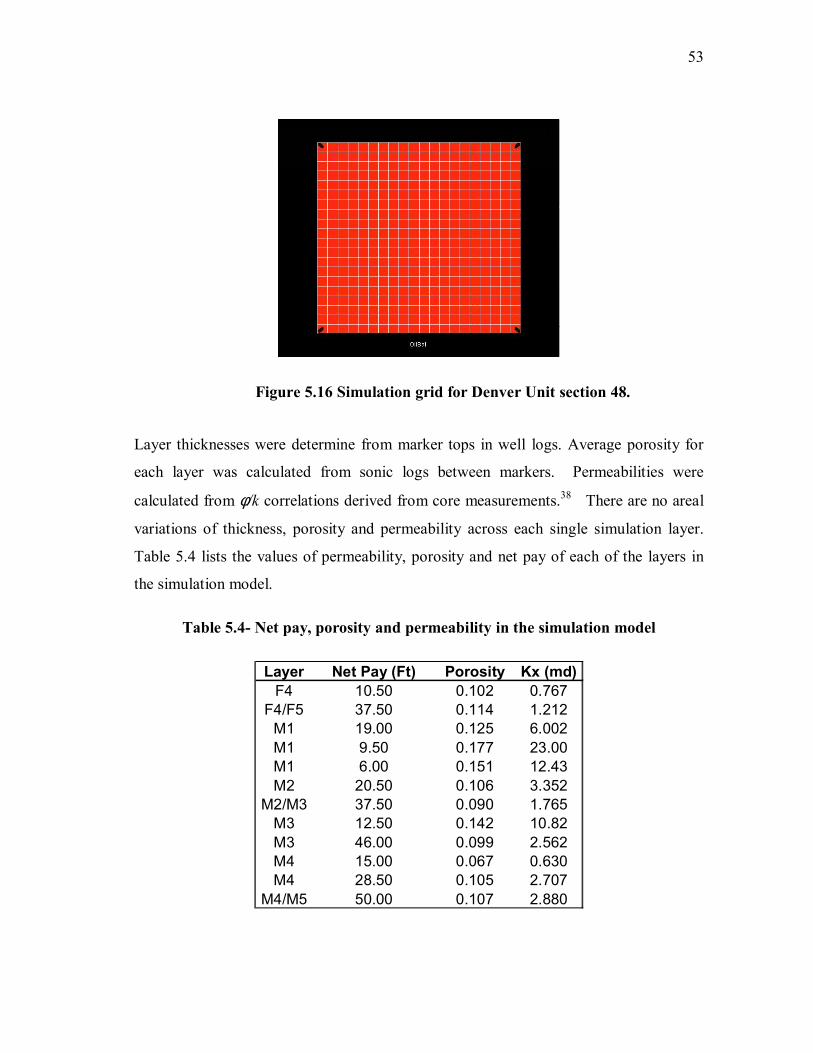
53

Injector

NS-Prod

EW-Prod

Diag-Prod

Injector

NS-Prod

EW-Prod

Diag-Prod

Figure 5.16 Simulation grid for Denver Unit section 48.

Layer thicknesses were determine from marker tops in well logs. Average porosity for

each layer was calculated from sonic logs between markers. Permeabilities were

calculated from φ/k correlations derived from core measurements.38 There are no areal

variations of thickness, porosity and permeability across each single simulation layer.

Table 5.4 lists the values of permeability, porosity and net pay of each of the layers in

the simulation model.

Table 5.4- Net pay, porosity and permeability in the simulation model

Layer Net Pay (Ft) Porosity Kx (md)F4 10.50 0.102 0.767

F4/F5 37.50 0.114 1.212M1 19.00 0.125 6.002M1 9.50 0.177 23.00M1 6.00 0.151 12.43M2 20.50 0.106 3.352

M2/M3 37.50 0.090 1.765M3 12.50 0.142 10.82M3 46.00 0.099 2.562M4 15.00 0.067 0.630M4 28.50 0.105 2.707

M4/M5 50.00 0.107 2.880

54

5.6 Initial Conditions

The reservoir model was initiated at a uniform pressure of 1,805 psia and constant

temperature of 105°F. The initial water saturation from the relative permeability curve

was 0.15. Initial oil saturation within the gridblocks was 0.85.

The geologic model provided an estimate of OOIP of 2.29 million bbls at initialization.

5.7 History Match

Usually the only way to test the validity of a model is to simulate past performance of

the reservoir and compare the simulation results with historical performance.

The pattern was history matched for both waterflood (from 1970 to mid 1986) and CO2

flood (from mid 1986 to 2004). The oil production and injection rates were specified in

each well and the model reproduced the reservoir pressure and the gas and water

production. The quality of the history match was judged from how well the simulated

water and gas production and reservoir pressure fitted historical data.

An important factor of the numerical modeling of the CO2 and water advance through

each of the layers was the understanding of the reservoir heterogeneities and the

identification of the main flow channels. This allowed for the identification of the

distribution of the remaining oil and gas in place.

For the history match, the relative permeability curves were slightly adjusted to obtain a

better producing water/oil ratio (WOR). The relative permeability curves were

normalized so that the end-point of the oil and water relative permeability at the connate

water saturation and the residual oil saturation was equal to 1.

Additionally, well connection factors to the simulation grid were because most of the

wells have been fractured and the wells�s permeability-thickness product, kh, and the

skin factor, S, were unknown. Since the connection factor is calculated from the cell

properties, cell geometry and completion information, modification of the connection

55

factor was accomplished by enlarging the completion interval of the production wells to

account for the effect of hydraulic stimulation.

During the WAG process, equal volumes of water and gas (at reservoir conditions) were

injected during each slug resulting in a WAG ratio of approximately 1. This WAG ratio

was kept constant for the CO2 flood history match.

During the waterflood period, water cut match is fairly good at early times. However, the

overall water production matches very well. A reasonable match of the gas production

was also obtained. Figure 5.17 through 5.19 contrast historical and simulated gas and

water production during the history match period.

Unfortunately, there is a lack of pressure data throughout the producing life of the

reservoir. The reservoir pressure in the pattern increases up to 3,150 psi during the

waterflood period, then decreases to 1,850 psi right before the CO2 injection starts.

According to previous studies on the production performance of the Denver Unit CO2

flood,39 the reservoir pressure was reduced from 3,200 psi to 2,200 psi in preparation for

the CO2 flood to improve the volumetric efficiency of the CO2. Figure 5.20 shows the

predicted average reservoir pressure performance for the model area.

Oil and water production from individual wells was also very good. The predicted

simulation production compared to actual production for the wells completed in the

pattern are shown in Figures 5.21 through 5.26. This indicates that the simulation model

was calibrated and can be used for making future predictions of reservoir performance.

56

0

100

200

300

400

500

600

700

0 5 10 15 20 25 30Years

Qg

(SC

F/D

)

Qg Sim Qg Hist

Figure 5.17- Gas production history match.

0

50

100

150

200

250

300

350

400

450

500

0 5 10 15 20 25 30Years

Qw

(STB

/D)

Simulated Hystorical

Figure 5.18- Water production history match.

57

0

10

20

30

40

50

60

70

80

90

0 5 10 15 20 25 30Years

Wat

er C

ut (%

)

Historical Simulated

Figure 5.19- Water cut history match.

0

500

1000

1500

2000

2500

3000

3500

4000

4500

5000

0 5 10 15 20 25 30Years

Pres

sure

, psi

Figure 5.20- Simulated reservoir pressure.

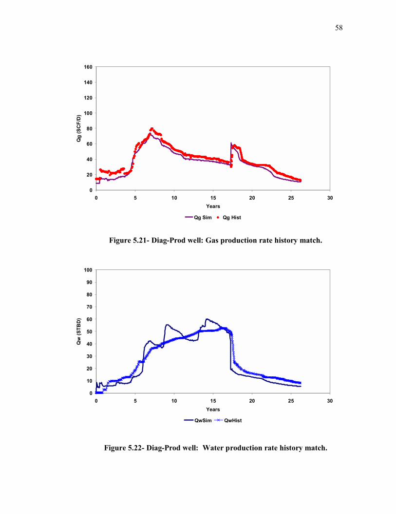
58

0

20

40

60

80

100

120

140

160

0 5 10 15 20 25 30Years

Qg

(SC

F/D

)

Qg Sim Qg Hist

Figure 5.21- Diag-Prod well: Gas production rate history match.

0

10

20

30

40

50

60

70

80

90

100

0 5 10 15 20 25 30Years

Qw

(STB

D)

QwSim QwHist

Figure 5.22- Diag-Prod well: Water production rate history match.

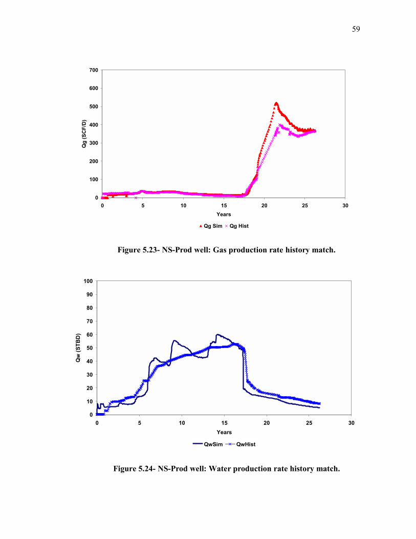
59

0

100

200

300

400

500

600

700

0 5 10 15 20 25 30Years

Qg

(SC

F/D

)

Qg Sim Qg Hist

Figure 5.23- NS-Prod well: Gas production rate history match.

0

10

20

30

40

50

60

70

80

90

100

0 5 10 15 20 25 30Years

Qw

(STB

D)

QwSim QwHist

Figure 5.24- NS-Prod well: Water production rate history match.

60

0

5

10

15

20

25

30

0 5 10 15 20 25 30Years

Qg

(MSC

FD)

Qg Hist Qg Sim

Figure 5.25- EW-Prod well: Gas production rate history match.

0

10

20

30

40

50

60

0 5 10 15 20 25 30Years

Qw

(STB

/D)

Qw Sim Qw Hist

Figure 5.26- EW-Prod well: Water production rate history match.

61

At the end of the history match period, layers F4 through M5, which initially contained

2.29 million STBO, had produced 893,862 STB or 39% of the OOIP, thus leaving a

remaining volume in place of 1.39 million STBO. The average remaining oil saturation

at the end of the history match was 45%. Figures 5.27 through 5.39 show the transition

of the distribution of the oil saturation during the history match period. Similarly,

Figures 5.40 through 5.52 show a cross-section view of oil saturation distribution in the

model throughout the history match.

The channeling of the injected fluids within the reservoir is clearly seen in the cross

sections. This causes a non-uniform movement of the front and therefore poor sweep

efficiency. High-permeability layers break through earlier than the low-permeability

layers, leaving some untapped reserves behind.

The pattern experienced a severe breakthrough that reduced the overall sweep efficiency

of the pattern. Additionally, little oil displacement was observed in the upper layers of

the San Andres Formation in the simulation model. The sweep efficiency of the patterns

was merely impacted by the contrast in permeability between the upper and lower layers

of the San Andres Formation. As a result, the injection well injected most of the fluids

into the lower layers even though the upper San Andres layers have commercial

permeability.

Results of the simulation not only highlighted reservoir areas with high oil saturation for

the future CO2 flooding but also reveal that mobility ratio needs to be improved and the

breakthrough has to be controlled to improve the injection profile and increase the

incremental oil recovery of the pattern.

62

Figure 5.27- Areal view of the oil saturation distribution. Year 0.

y

xINJ

EW_PROD DIAG_PROD

NS_PROD

Oil Saturation0.0 0.21 0.42 0.643 0.85

y

x

y

xINJ

EW_PROD DIAG_PROD

NS_PRODINJ

EW_PROD DIAG_PROD

NS_PROD

Oil Saturation0.0 0.21 0.42 0.643 0.85

Oil Saturation0.0 0.21 0.42 0.643 0.85


y

xINJ

EW_PROD DIAG_PROD

NS_PROD

Oil Saturation0.0 0.21 0.42 0.643 0.85

y

x

y

INJ

EW_PROD DIAG_PROD

NS_PRODINJ

EW_PROD DIAG_PROD

NS_PROD

Oil Saturation0.0 0.21 0.42 0.643 0.85

Oil Saturation0.0 0.21 0.42 0.643 0.85

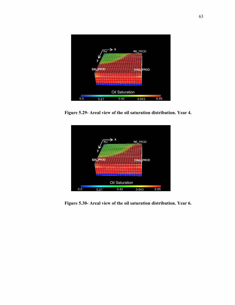
63

y

xINJ

EW_PROD DIAG_PROD

NS_PROD

Oil Saturation0.0 0.21 0.42 0.643 0.85

y

x

y

xINJ

EW_PROD DIAG_PROD

NS_PRODINJ

EW_PROD DIAG_PROD

NS_PROD

Oil Saturation0.0 0.21 0.42 0.643 0.85

Oil Saturation0.0 0.21 0.42 0.643 0.85


y

xINJ

EW_PROD DIAG_PROD

NS_PROD

Oil Saturation0.0 0.21 0.42 0.643 0.85

y

x

y

xINJ

EW_PROD DIAG_PROD

NS_PRODINJ

EW_PROD DIAG_PROD

NS_PROD

Oil Saturation0.0 0.21 0.42 0.643 0.85

Oil Saturation0.0 0.21 0.42 0.643 0.85


64

y

xINJ

EW_PROD DIAG_PROD

NS_PROD

Oil Saturation0.0 0.21 0.42 0.643 0.85

y

x

y

xINJ

EW_PROD DIAG_PROD

NS_PRODINJ

EW_PROD DIAG_PROD

NS_PROD

Oil Saturation0.0 0.21 0.42 0.643 0.85

Oil Saturation0.0 0.21 0.42 0.643 0.85


y

xINJ

EW_PROD DIAG_PROD

NS_PROD

Oil Saturation0.0 0.21 0.42 0.643 0.85

y

x

y

xINJ

EW_PROD DIAG_PROD

NS_PRODINJ

EW_PROD DIAG_PROD

NS_PROD

Oil Saturation0.0 0.21 0.42 0.643 0.85

Oil Saturation0.0 0.21 0.42 0.643 0.85


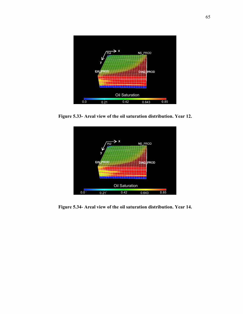
65

y

xINJ

EW_PROD DIAG_PROD

NS_PROD

Oil Saturation0.0 0.21 0.42 0.643 0.85

y

x

y

xINJ

EW_PROD DIAG_PROD

NS_PRODINJ

EW_PROD DIAG_PROD

NS_PROD

Oil Saturation0.0 0.21 0.42 0.643 0.85

Oil Saturation0.0 0.21 0.42 0.643 0.85


y

xINJ

EW_PROD DIAG_PROD

NS_PROD

Oil Saturation0.0 0.21 0.42 0.643 0.85

y

x

y

xINJ

EW_PROD DIAG_PROD

NS_PRODINJ

EW_PROD DIAG_PROD

NS_PROD

Oil Saturation0.0 0.21 0.42 0.643 0.85

Oil Saturation0.0 0.21 0.42 0.643 0.85


66

y

xINJ

EW_PROD DIAG_PROD

NS_PROD

Oil Saturation0.0 0.21 0.42 0.643 0.85

y

x

y

xINJ

EW_PROD DIAG_PROD

NS_PRODINJ

EW_PROD DIAG_PROD

NS_PROD

Oil Saturation0.0 0.21 0.42 0.643 0.85

Oil Saturation0.0 0.21 0.42 0.643 0.85


y

xINJ

EW_PROD DIAG_PROD

NS_PROD

Oil Saturation0.0 0.21 0.42 0.643 0.85

y

x

y

xINJ

EW_PROD DIAG_PROD

NS_PRODINJ

EW_PROD DIAG_PROD

NS_PROD

Oil Saturation0.0 0.21 0.42 0.643 0.85

Oil Saturation0.0 0.21 0.42 0.643 0.85


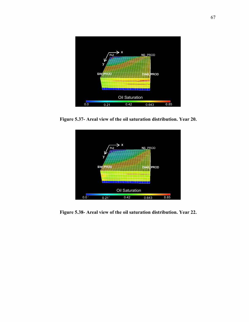
67

y

xINJ

EW_PROD DIAG_PROD

NS_PROD

Oil Saturation0.0 0.21 0.42 0.643 0.85

y

x

y

xINJ

EW_PROD DIAG_PROD

NS_PRODINJ

EW_PROD DIAG_PROD

NS_PROD

Oil Saturation0.0 0.21 0.42 0.643 0.85

Oil Saturation0.0 0.21 0.42 0.643 0.85


y

xINJ

EW_PROD DIAG_PROD

NS_PROD

Oil Saturation0.0 0.21 0.42 0.643 0.85

y

x

y

xINJ

EW_PROD DIAG_PROD

NS_PRODINJ

EW_PROD DIAG_PROD

NS_PROD

Oil Saturation0.0 0.21 0.42 0.643 0.85

Oil Saturation0.0 0.21 0.42 0.643 0.85


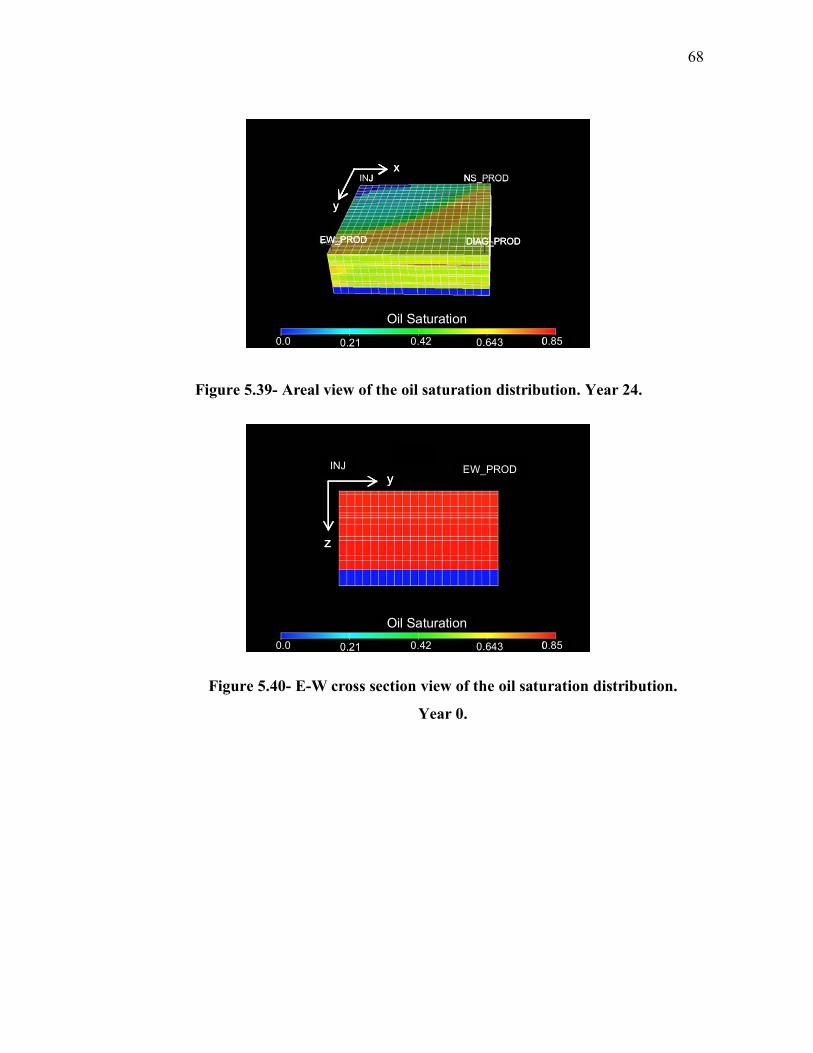
68

y

xINJ

EW_PROD DIAG_PROD

NS_PROD

Oil Saturation0.0 0.21 0.42 0.643 0.85

y

x

y

xINJ

EW_PROD DIAG_PROD

NS_PRODINJ

EW_PROD DIAG_PROD

NS_PROD

Oil Saturation0.0 0.21 0.42 0.643 0.85

Oil Saturation0.0 0.21 0.42 0.643 0.85


Oil Saturation0.0 0.21 0.42 0.643 0.85

INJ EW_PRODy

z

Oil Saturation0.0 0.21 0.42 0.643 0.85

Oil Saturation0.0 0.21 0.42 0.643 0.85

INJ EW_PRODINJ EW_PRODy

z

y

z

Figure 5.40- E-W cross section view of the oil saturation distribution.

Year 0.

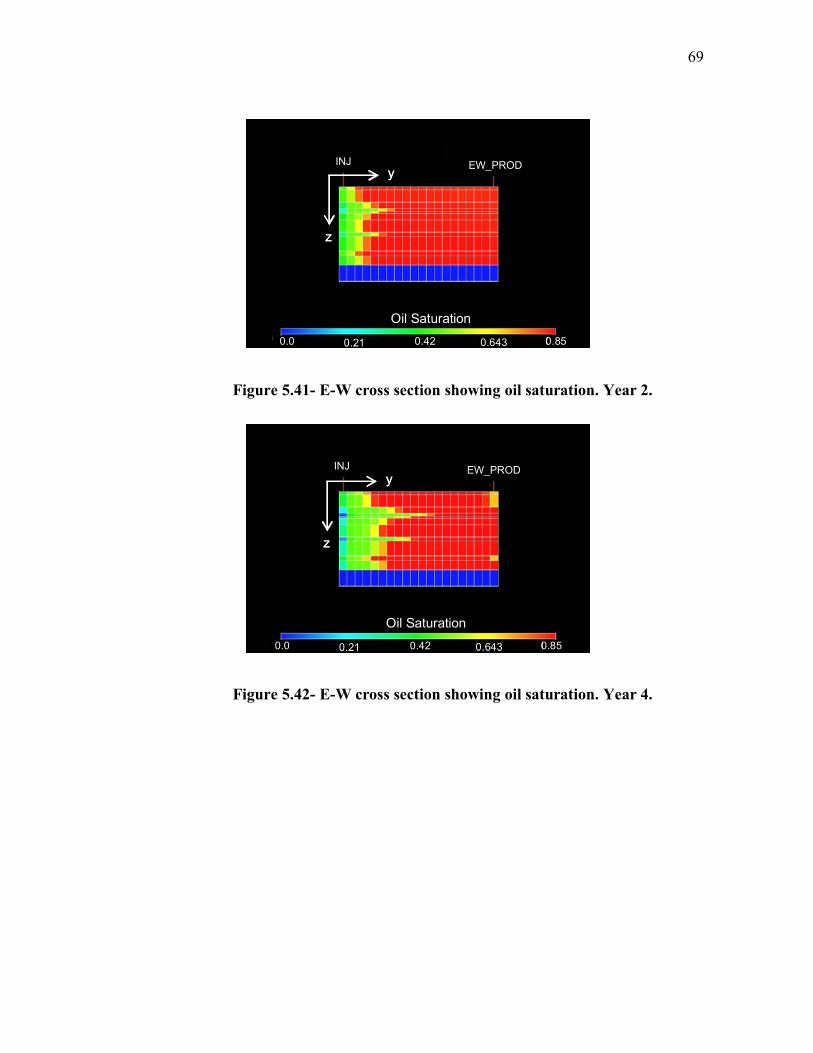
69

Oil Saturation0.0 0.21 0.42 0.643 0.85

INJ EW_PRODy

z

Oil Saturation0.0 0.21 0.42 0.643 0.85

Oil Saturation0.0 0.21 0.42 0.643 0.85


z

y

z

Figure 5.41- E-W cross section showing oil saturation. Year 2.

Oil Saturation0.0 0.21 0.42 0.643 0.85

INJ EW_PRODy

z

Oil Saturation0.0 0.21 0.42 0.643 0.85

Oil Saturation0.0 0.21 0.42 0.643 0.85


z

y

z


70

Oil Saturation0.0 0.21 0.42 0.643 0.85

INJ EW_PRODy

z

Oil Saturation0.0 0.21 0.42 0.643 0.85

Oil Saturation0.0 0.21 0.42 0.643 0.85


z

y

z


Oil Saturation0.0 0.21 0.42 0.643 0.85

INJ EW_PRODy

z

Oil Saturation0.0 0.21 0.42 0.643 0.85

Oil Saturation0.0 0.21 0.42 0.643 0.85


z

y

z


71

Oil Saturation0.0 0.21 0.42 0.643 0.85

INJ EW_PRODy

z

Oil Saturation0.0 0.21 0.42 0.643 0.85

Oil Saturation0.0 0.21 0.42 0.643 0.85


z

y

z


Oil Saturation0.0 0.21 0.42 0.643 0.85

INJ EW_PRODy

z

Oil Saturation0.0 0.21 0.42 0.643 0.85

Oil Saturation0.0 0.21 0.42 0.643 0.85


z

y

z


72

Oil Saturation0.0 0.21 0.42 0.643 0.85

INJ EW_PRODy

z

Oil Saturation0.0 0.21 0.42 0.643 0.85

Oil Saturation0.0 0.21 0.42 0.643 0.85


z

y

z


Oil Saturation0.0 0.21 0.42 0.643 0.85

INJ EW_PRODy

z

Oil Saturation0.0 0.21 0.42 0.643 0.85

Oil Saturation0.0 0.21 0.42 0.643 0.85


z

y

z


73

Oil Saturation0.0 0.21 0.42 0.643 0.85

INJ EW_PRODy

z

Oil Saturation0.0 0.21 0.42 0.643 0.85

Oil Saturation0.0 0.21 0.42 0.643 0.85


z

y

z


Oil Saturation0.0 0.21 0.42 0.643 0.85

INJ EW_PRODy

z

Oil Saturation0.0 0.21 0.42 0.643 0.85

Oil Saturation0.0 0.21 0.42 0.643 0.85


z

y

z


74

Oil Saturation0.0 0.21 0.42 0.643 0.85

INJ EW_PRODy

z

Oil Saturation0.0 0.21 0.42 0.643 0.85

Oil Saturation0.0 0.21 0.42 0.643 0.85


z

y

z


INJ EW_PRODy

z


z

y

z


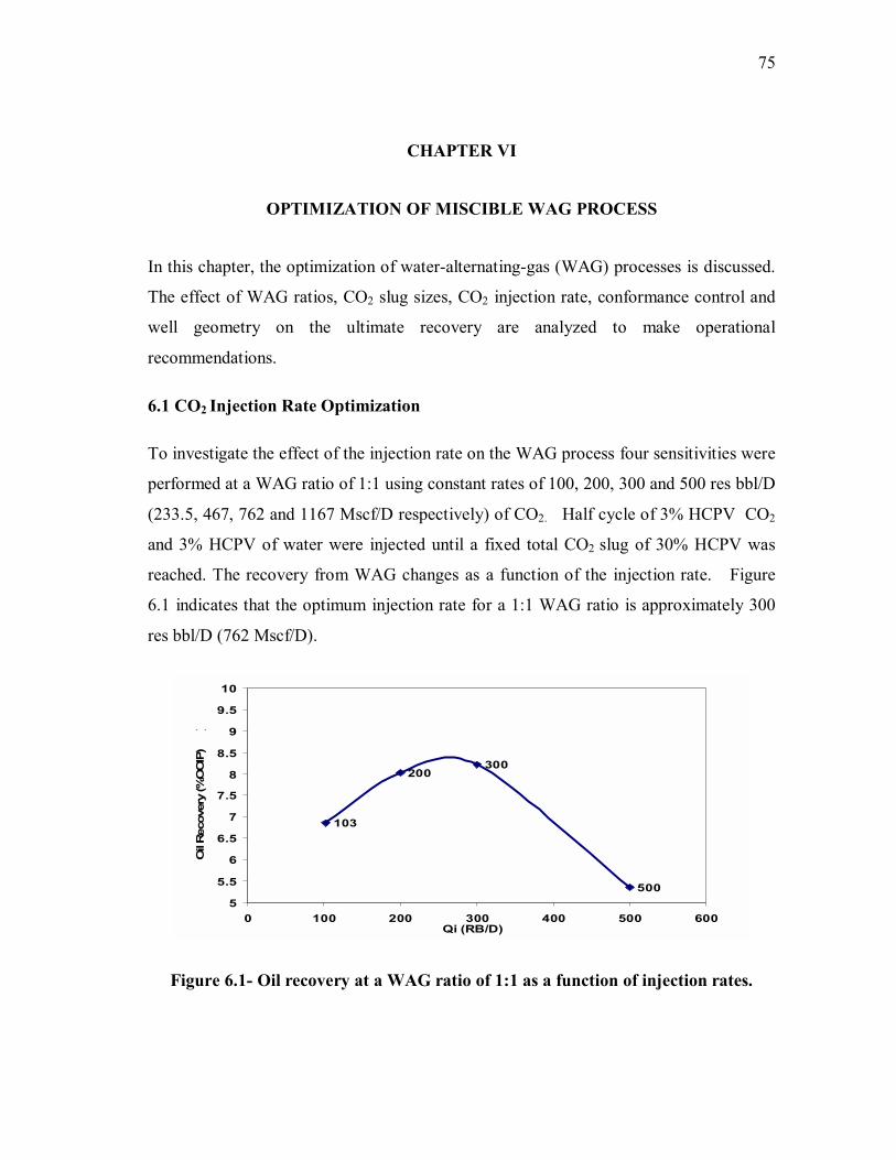
75

CHAPTER VI

4. OPTIMIZATION OF MISCIBLE WAG PROCESS

In this chapter, the optimization of water-alternating-gas (WAG) processes is discussed.

The effect of WAG ratios, CO2 slug sizes, CO2 injection rate, conformance control and

well geometry on the ultimate recovery are analyzed to make operational

recommendations.

6.1 CO2 Injection Rate Optimization

To investigate the effect of the injection rate on the WAG process four sensitivities were

performed at a WAG ratio of 1:1 using constant rates of 100, 200, 300 and 500 res bbl/D

(233.5, 467, 762 and 1167 Mscf/D respectively) of CO2. Half cycle of 3% HCPV CO2

and 3% HCPV of water were injected until a fixed total CO2 slug of 30% HCPV was

reached. The recovery from WAG changes as a function of the injection rate. Figure

6.1 indicates that the optimum injection rate for a 1:1 WAG ratio is approximately 300

res bbl/D (762 Mscf/D).

103

200300

5005

5.5

6

6.5

7

7.5

8

8.5

9

9.5

10

0 100 200 300 400 500 600Qi (RB/D)

Oil

Rec

over

y (%

OO

IP)

)

Figure 6.1- Oil recovery at a WAG ratio of 1:1 as a function of injection rates.

76

6.2 Optimum Water-Alternating-Gas (WAG) Ratio

Two of the most important design issues for WAG process optimization are the WAG

ratio and the amount of gas injection or slug size. Various compositional simulations

were conducted to determine the optimum WAG ratio and the optimum slug size.

A series of WAG ratio sensitivities were compared. Water alternating with CO2

injections at four different WAG ratios (1:1, 1:2, 2:1, and 4:1) were performed. The runs

evaluated CO2 slug sizes up to 100% HCPV. The gas and water injections were carried

out in cycles, injecting both fluids in the same well.

Model results showed sensitivity to the WAG ratio used. Results indicate that injecting

a 100% hydrocarbon pore volume (HCPV) slug of CO2 with a 1:1 WAG ratio would

yield the maximum incremental oil recovery. The design included injection of

alternating volumes (3.0% HCPV) of CO2 and water into each pattern until the target

100% slug size was reached.

Figure 6.2 shows the CO2 flood performance for the different WAG ratios as a function

of total CO2 injection. The recovery profiles indicate that the best incremental oil

recovery is obtained at a WAG ratio of 1:1. As shown in figure 6.2, the highest recovery

is obtained at the smallest WAG ratio during the optimization process. Much of the oil

obtained with high WAG ratios is recovered at a very high and uneconomical water cut

(>95%), even though the planned CO2 slug size had not been injected.

A continuous CO2 flood and waterflooding recovery profiles are also shown in Figure

6.2 for comparison. The incremental oil recovery obtained with the continuous CO2

flood was low. CO2 injected this way broke through the high permeability layers of the

pattern.

Figure 6.3 shows the residual oil saturation in the reservoir for all the cases after 100%

HCPV have been injected. As expected, the 1:1 WAG ratio exhibits the lowest

remaining oil saturation.

77

Figure 6.2- Comparison of different WAG ratios in terms of the incremental

oil recovery as a function of the CO2 slug size.

0.26 0.27

0.280.29

0.34 0.33

0.20

0.22

0.24

0.26

0.28

0.30

0.32

0.34

0.36

WAG 1:1 WAG 1:2 WAG 2:1 WAG 4:1 Waterflooding Continuos CO2

Sor

Residual Oil Saturation

Figure 6.3- Comparison of the residual oil saturation for various WAG ratios after

injection of 100% HCPV of CO2.

78

6.3 Conformance Control

Channeling of the injected CO2 during a WAG process has been a major area of concern

in the oil industry.30 During the course of CO2 injection multiple profile control

treatments have been conducted to improve the sweep efficiency.

To reduce the CO2 mobility and delay the breakthrough of the CO2, simulations of

polymer injection and a blocking agent treatments were performed with a WAG ratio of

1:1. Polymer injection reduces CO2 cycling through a high-permeability layer between

the injection well and offset producing wells. This simulation allowed for the

investigation of the effect of these treatments on the sweep efficiency and conformance

control.

To simulate the effect of placing the surfactant in the �thief� zone, a high-permeability

layer was identified (layer 4, M1 formation) in the simulation model and the gridblock

next to the injector well was plugged by assigning it a zero permeability value. See

Figure 6.4.

Polymers have been used at CO2 WAG injection wells to form an in-situ gel. The gel

must be selectively injected so that it flows to the most permeable zones. After a certain

amount of time, the gel stiffens and blocks fluid through those zones.

For the polymer injection treatment, the injected water viscosity was increased from 1 to

20 cps. For this run, care was taken not to increase the injection pressure above the

formation parting pressure where it might subsequently create an injection-induced

fracture. As can be noted from Figure 6.5, the injection pressure is between 3,100 and

3,900 psi during the process.

79

Permeability

0.0 5.7 11.5 17.2 23

K=0

Inj Prod

Permeability

0.0 5.7 11.5 17.2 23

K=0K=0

Inj Prod

Figure 6.4- East �West cross section view of the simulation model showing the

permeability block by the polymer.

Production rates before and after the treatments were compared (Figure 6.6). The oil

production rate of the pattern exhibits a significant response to the profile control

treatments performed on the injection well. However, the effectiveness of the treatments

does not last long (in time) and the production rate declines quickly after the treatments,

which indicate that the positive effects of the treatments are not permanent.

80

2500

2700

2900

3100

3300

3500

3700

3900

4100

0 1 2 3 4 5 6 7 8 9 10Years

Pres

sure

, psi

a

Figure 6.5- Injection pressure profile during the viscous water treatment.

0

20

40

60

80

100

120

140

160

180

0 5 10 15 20 25 30 35 40 45 50Years

Qo

(STB

/D)

Gel No treatment Polymer History

Polymer

Gel

No treatment

0

20

40

60

80

100

120

140

160

180

0 5 10 15 20 25 30 35 40 45 50Years

Qo

(STB

/D)

Gel No treatment Polymer History

Polymer

Gel

No treatment

Figure 6.6- Comparison of conformance control treatments as a function of oil

production rate.

81

Figure 6.7 shows the effect of the conformance control on the incremental recovery as a

function of the volume of CO2 injected. The incremental recovery obtained from the

polymer injection and the viscous water treatments is compared to the recovery obtained

from a WAG 1:1 ratio injection process without any treatment.

Even though results indicate that the application of these treatments can significantly

increase the oil production, the success of this technique in the field will depend on the

correct placement of the polymer without damaging other adjacent layers. Additionally,

it depends on the periodic repetition of the treatment to positively affect areal sweep

efficiency.

0.0

5.0

10.0

15.0

20.0

25.0

30.0

35.0

0.00 10.00 20.00 30.00 40.00 50.00 60.00 70.00 80.00 90.00 100.00CO2 Slug, %HCPV

Incr

emen

tal R

ecov

ery,

%O

OIP

Polymer No treatment Gel

Figure 6.7- Comparison of conformance control treatments in terms of the

incremental oil recovery as a function of the CO2 slug size.

82

6.4 Optimum Well Pattern

This section analyzes the effect of pattern reconfiguration on the CO2 displacement.

Pattern conversion is a viable option to achieve an incremental recovery in a mature field

with high remaining oil saturations.

A pattern reconfiguration can improve the performance by improving the geometry,

decreasing the spacing of the patterns, reducing the producer/injector ratio, and hence

improving areal and vertical efficiency.

This sensitivity includes infill drilling and well conversion from producer to injector to

achieve a better CO2 displacement throughout the reservoir and ultimately obtain a

substantial increase in production from the existing CO2 flood.

Different well configurations were simulated and analyzed. The typical Denver Unit

inverted nine-spot pattern was converted to a staggered line-drive pattern, a line-drive

pattern and a nine-spot pattern in the simulation model.

The new patterns were forecast using the saturations and pressures at the end of the

history match. Figure 6.8 shows the geometric patterns considered in this work. The

gridded zone represents the simulated area of the full pattern

Injector ProducerInjector ProducerProducer

Figure 6.8- (a) Staggered line drive, (b) line drive and (c) nine-spot well

patterns.

83

For the staggered-line-drive pattern, the EW-Prod production well was converted into an

injection well and a new production (infill) well was incorporated. With this well

configuration, the well spacing was modified from 20 acres to 10 acres. The new injector

well was set up to inject water alternating CO2 at a WAG ratio of 1:1.

To create a line-drive pattern, a new injector well was incorporated in the model and

aligned with the other injectors in the staggered-line-drive pattern as shown in Figure

6.8. For the nine-spot pattern, a single producer well and three injectors were kept in the

model.

Figure 6.9 compares the production performance obtained from each pattern

investigated. The figure also shows a plot of the actual production rate of the pattern.

The sharp rise in the production rate is very evident after redefining the well pattern

geometry to staggered-line-drive and line-drive patterns. Simulation results showed both

the staggered-line-drive pattern and the line-drive pattern create an immediate peak

above 100 STB/D in the production rate, which represents approximately a 66% of

increase in production as a result of the pattern reconfiguration.

0

20

40

60

80

100

120

140

160

180

0 5 10 15 20 25 30 35 40 45 50Years

Qo

(STB

/D)

Inverted 9-Spot Line Drive Stag. Line Drive 9 Spot

Staggerered line drive

Line drive

Nine-spot

Inverted nine-spot

Figure 6.9-Comparison of staggered-line-drive, line-drive and nine-spot well

patterns.

84

The production rates obtained from the inverted nine-spot pattern is the lowest one

among the patterns compared here. Extremely low rates clearly indicate that this pattern

configuration does not perform well for this particular drainage area and does not

improve the CO2 displacement.

85

CHAPTER VII

CONCLUSIONS

1) Recovery from a WAG process is a function of the injection rate as well as WAG

ratio and the CO2 slug.

2) WAG injection is effective in increasing the sweep efficiency of the injected CO2 in

the reservoir.

3) Simulation showed that Denver Unit tertiary CO2 flood would have a maximum

recovery of 18% at a 1:1 WAG ratio and a CO2 slug size of 100% HCPV.

4) The optimal injection rate for the pattern is 300 RB/D of CO2 at a WAG 1:1 ratio.

5) The injection of viscous water and polymer resulted in a positive production response

that yielded an incremental oil recovery of 32% and 20% respectively.

6) Modeling suggests that pattern conversion form the typical Denver Unit inverted

nine-spot pattern to staggered-line-drive improves the production oil rate in 66%.

7) The CO2 pattern modeling provides guidance in the reservoir management in the

Wasson Field, San Andres Formation in the Denver Unit.

86

5. NOMENCLATURE

Z = gas deviation factor φ = porosity µ = viscosity, cp ρ = fluid density, lbm/ft3

q= production rate FVF= formation volume factor GOR=Gas-oil ratio Subscripts g = gas w= water o= oil

87

6. REFERENCES

1. Fleming, E.A., Brown, L.M. and Cook, R.L.: �Overview of Production Engineering Aspects of Operating the Denver Unit CO2 flood,� paper SPE/DOE 24157 presented at the 1992 SPE/DOE Symposium on Improved Methods for Oil Recovery, Tulsa, OK, 22-24 April

2. Hsu, C.F., Morell, J.I. and Falls, A.H.: �Field Scale CO2 Flood Simulations and Their Impact on the Performance of the Wasson Denver Unit,� paper SPE 29116 presented at the 1995 SPE Symposium on Reservoir Simulation, San Antonio, TX, 12-15 February.

3. Ghauri, W.K.: �Production Technology Experience in a Large Carbonate Waterflood, Denver Unit, Wasson San Andres Field,� paper SPE 8406 presented at the 54th Annual Technical Conference and Exhibition held in Las Vegas, NV. Sept. 23-26, 1979.

4. Thai, B.N., Hsu, C.F., Bergersen, B.M., Albrecht, S,L., and Richardson, T.W.: �Denver Unir Infill and Pattern Reconfiguration Program,� paper SPE 59548 presented at the 2000 SPE Permian Basin Oil and Gas Recovery Conference, Midland, TX, 21-23 March.

5. Mathis, R.L.: �Effect of CO2 Flooding on Dolomite Reservoir Rock, Denver Unit, Wasson (San Andres) Field, TX,� paper SPE 13132 presented at the 59th

Annual Technical Conference and Exhibition, Houston, TX, 16-19 September.

6. Martin, F.D. and Taber, J.J.: �Carbon Dioxide Flooding,� SPE Technology Today Series (April 1992) 396 � 400.

7. Jarrel, P.M., Fox, C.E., Stein., M.H. and Webb, S.L.: F.: Practical Aspects of CO2 Flooding, Monograph Series, SPE, Richardson, Texas (2002).

8. Caudle, B.H. and Dyes, A.B.: �Improving Miscible Displacement by Gas-Water Injection�, Transactions of AIME, (1959) 213, 281-284.

9. Huang, E.T.S. and Holm, L.W.: �Effect of WAG Injection and Rock Wettability on Oil Recovery During CO2 Flooding,� SPERE (Feb. 1988) 119-129.

10. Green, D.W. and Willhite, P.: Enhanced Oil Recovery SPE Textbook Series, Richardson, Texas (1998).

88

11. Sanchez, N.L.: �Management of Water Alternating (WAG) Injection Projects,� paper SPE 53714 presented at the 1999 Latin American and Caribbean Petroleum Engineering Conference, Caracas, Venezuela, 21-23 April.

12. Christensen, J R, Stenby, E H, and Skauge, A,.: �Review of the WAG Field Experience�, paper SPE 71203, presented at the 1998 SPE International Petroleum Conference and Exhibition of Mexico, Villa Hermosa, 3-5 March.

13. Bellavance, J.F.R.: �Dollarhide Devonian CO2 Flood: Project Performance Review 10 Years Later,� paper SPE 35190 presented at the 1996 SPE Permian Basin Oil and Gas Recovery Conference, Midland, TX, 27-29 March.

14. Tanner, C.S. and Baxley, P.T.: �Production Performance of the Wasson Denver Unit CO2 Flood,� paper SPE 24156 presented at the 1992 Enhanced Oil Recovery Symposium,Tulsa, OK, 22-24 April.

15. Kulkarni, M. M. and Rao, D. N.: �Experimental Investigation of Various Methods of Tertiary Gas Injection�, SPE 90589, paper presented at the 2004 Society of Petroleum Engineers Annual Technical Conference and Exhibition, Houston, TX, 26 � 29, Sept.

16. Jackson, D.D., Andrews, G.L., and Claridge, E.L.: �Optimum WAG Ratio vs. Rock Wettability in CO2 Flooding,� paper SPE 14303 presented at the 1985 Annual Technical Conference and Exhibition, Las Vegas, NV, 22-25 September.

17. Gorrell, S.B.: �Implications of Water-Alternate-Gas Injection, for Profile Control and Injectivity,� paper SPE 20210 presented at the 1990 SPE/DOE Seventh Symposium on Enhanced Oil Recovery, Tulsa, OK, 22-25 April.

18. Rogers, J.D., Reid B. and Grigg, R.B.: �A Literature Analysis of the WAG Injectivity Abnormalities in the CO2 Process,� paper SPE 59329 presented at the 2000 Improved Oil Recovery Symposium, Tulsa, OK, 3-5 April.

19. M.K. Roper Jr., Pope, G.A., and Sepehrnoori, K.: �Analysis of Tertiary Injectivity of Carbon Dioxide," paper SPE 23974, presented at the proceedings of the SPE Permian Basin Oil and Gas Recovery Conference, Midland, TX, March 18-20, 1992.

20. Christman, P.G. and Gorell, S.B.: �A Comparison of Laboratory and Field-Observed CO2 Tertiary Injectivity,� paper SPE/DOE 17335 presented at the 1988 Improved Oil Recovery Symposium., Tulsa, OK,17-20 April.

21. Bennion, D.B., Thomas, F.B., Jamaluddin, A.K.M. and Ma, T.: �The Effect of Trapped Critical Fluid Saturations on Reservoir Permeability and Conformance,�

89

paper presented at the 1998 Annual Technical Meeting of the Petroleum Society of CIM, Calgary, Alberta, Canada, 8 -10 June.

22. Harpole, K.J. and Hallenbeck, L.D.: �East Vacuum Grayburg San Andres Unit CO2 Flood Ten Year Performance Review: Evolution of a Reservoir Management Strategy and Results of WAG Optimization,� paper SPE 36710 presented at the 1996 Annual Technical Conference and Exhibition, Denver, CO, 6-9 October.

23. Lemen, M.A., Burlas, T.C., and Roe, L.M.: �Waterflood Pattern Realignment at the McElroy Field: Section 205 Case History,� paper SPE 20120 presented at the 1990 Permian Basin Oil and Gas Recovery Conference, Midland, TX, 8-9 March.

24. Pariani, G.J., McColloch, K.A., and Warden, S.L.: �An Approach to Optimize Economics in a West Texas CO2 Flood,� paper SPE 22022 presented at the Hydrocarbon Economics and Evaluation Symposium, Dallas, TX, 11-12 April.

25. Shing-Ming C., Allard, D.R., and Anli, J.: �Factors Affecting Solvent Slug Size Hydrocarbon Miscible Flooding Requirements in Hydrocarbon Miscible Flooding,� SPE paper 12636 presented at the 4th Symposium on Enhanced Oil Recovery, Tulsa, OK,15-18, April.

26. Hadlow, R.E.: �Update of Industry Experience with CO2 Injection,� paper SPE 24928 presented at the 1992 SPE Annual Technical Conference and Exhibition, Washington, D.C, 4-7 October.

27. Gharbi-Ridha, B.C., �Integrated Reservoir Simulation Studies to Optimize Recovery from a Carbonate Reservoir,� paper SPE 80437 presented at the SPE Asia Pacific Oil and Gas Conference and Exhibition, Jakarta, Indonesia, 9-11 September.

28. Holm, W. L.: �Evolution of the Carbon Dioxide Flooding Processes,� Oil and Gas Journal, (November 1987) 1337.

29. Seright, R.S.: �Placement of Gels to Modify Injection Profiles,� paper SPE/DOE 17332 presented at the 1988 SPE/DOE Enhanced Oil Recovery Symposium, Tulsa, OK, 17-20 April.

30. Vela, S., Peaceman, D.W., and Sandvik, E.I.: �Evaluation of Polymer Flooding in a Layered Reservoir with Crossflow, Retention, and Degradation,� SPEJ (April 1976) 82.

90

31. Mathis, R.L.: �Reservoir Geology of the Denver Unit � Wasson San Andres Field, Gaines and Yoakum Counties, Texas,� Permian Basin SEPM Publication 86-26, 1986, 43-47.

32. Schneider, W. T.: �Geology of Wasson Field, Yoakum and Gaines Counties, Texas,� Bulletin of the American Association of Petroleum Geologists (April 1943), 27.

33. Mathis, R.L.: �Effect of CO2 Flooding on Dolomite Reservoir Rock, Denver Unit, Wasson (San Andres) Field, TX,� paper SPE 13132 presented at the 1984 Annual Technical Conference and Exhibition, Houston, TX, September 16-19.

34. P. E. Cowan and P. M. Harris, "Porosity Distribution in San Andres Formation (Permian), Cochran and Hockley Counties, Texas," Bulletin of the American Association of Petroleum Geologists (July 1986), 70.

35. Galloway, W. E., Ewing, T. E., Garrett, C. M., Jr., Tyler, Noel, and Bebout, D. G., Atlas of Major Texas Oil Reservoirs, The University of Texas at Austin, Bureau of Economic Geology, (1983).

36. Purves, W. J., Reservoir Description of the Mobil Oil Bridges State Leases (Upper San Andres reservoir), Vacuum Field, Lea County, New Mexico, in Bebout, D. G., and Harris, P. M., eds., Geologic and Engineering Approaches in Evaluation of San Andres/Grayburg Hydrocarbon Reservoirs�Permian Basin, The University of Texas at Austin, Bureau of Economic Geology, (1986) p, 87�112.

37. Loucks, R. G., Mescher, P., Entzminger, D., and Braaten, D, 2003, �Reservoir Geology of the Willard Unit in the San Andres Wasson Field, West Texas,� Southwest Section American Association of Petroleum Geologists Convention, Fort Worth, TX, March 1�5.

38. Swift, T.E., Goodrich, J., Kumar, R. and McCoy, R.L; �San Andres Reservoir Pressure Coring Project for Enhanced Oil Recovery Evaluation, Bennett Ranch Unit, Wasson Field, West Texas,� paper SPE/DOE 9798 presented at the 1981 SPE/DOE Second Joint Symposium on Enhanced Oil Recovery, Tulsa, OK, 5-8 April.

39. Tanner, C.S., and Baxley, P.T.: �Production Performance of the Wasson Denver Unit CO2 Flood,� paper SPE 24156 presented at the 1992 Enhanced Oil Recovery Symposium, Tulsa, OK, 22-24 April.

40. Kittridge, M.G.: �Quantitative CO2 Flood Monitoring, Denver Unit, Wasson (San Andres) Field,� paper SPE 24644 presented at the 67th Annual Technical Conference and Exhibition, Washington, DC, October 4-7, 1992.

91

41. ECLIPSE 300 Reference Manual, 2004A-1 Release, Schlumberger Reservoir Technologies, Houston, TX 77056 (2004).

42. Merrill, R.C., Hartman, K.J. and Creek, J.L.: �A Comparison of Equation of State Tuning Methods,� paper SPE 28589 presented at the 69th Annual Technical and Exhibition New Orleans, LA, 25-28 September.

43. Khan, S.A., Pope, G.A. and Sepehrnoori, K.: �Fluid Characterization of Three-Phase CO2/Oil Mixtures,� paper SPE/DOE 24130 presented at the 8th Symposium Oil Recovery, Tulsa, OK, 22-24 April, 1992.

44. Peng, D.Y. and Robinson, D.B.: �A New Two-Constant Equation of State,� Ind. & Eng. Chem. Fund. (1976) 15, No. 1, 59-64.

45. Lohrenz, J., Bray, B.G. and Clark, C.R.: �Calculating Viscosities of Reservoir Fluids from Their Compositions,� J. Pet. Tech. (Oct. 1964) 16, 1171-1176.

46. Whitson, C.H.: �Characterizing Hydrocarbon Plus Fraction,� SPEJ, 23, (1983), 683-684.

47. Fevang, O., Singh, K. and Whitson, C.H.: �Guidelines for Choosing Compositional and Black-Oil Models for Volatile Oil and Gas Condensate Reservoirs,� paper SPE 63087 presented at the 2000 SPE Annual Technical Conference and Exhibition, Dallas, TX, 1-4 October.

48. Bennion, D.B., Thomas, F.B., Jamaluddin, A.K.M., and Ma, T.: �The Effect of Trapped Critical Fluid Saturations on Reservoir Permeability and Conformance.� Presented at the 1998 Annual Technical Meeting of the Petroleum Society of CIM, Calgary, Alberta, Canada, 8 -10 June

92

VITA

Name : Marylena Garcia Quijada

Permanent Address : 5510 S Rice Avenue # 1614 Houston TX 77081 Email : [email protected]

Education : B.S., Petroleum Engineering, Universidad de Oriente, Barcelona, Venezuela, (November 1998)

M.S., Petroleum Engineering, Texas A&M University, College Station, TX 77843-3116, U.S.A. (August 2005)

OPTIMIZATION OF A CO FLOOD DESIGN WASSON FIELD - WEST...

Documents

Transcript of OPTIMIZATION OF A CO FLOOD DESIGN WASSON FIELD - WEST...