Optimization Methods for Convolutional Sparse Coding

Hilton Bristow · Simon Lucey

June 11, 2014

Abstract Sparse and convolutional constraints form a

natural prior for many optimization problems that arise

from physical processes. Detecting motifs in speech

and musical passages, super-resolving images, com-

pressing videos, and reconstructing harmonic motions

can all leverage redundancies introduced by convo-

lution. Solving problems involving sparse and convo-

lutional constraints remains a difficult computational

problem, however. In this paper we present an overview

of convolutional sparse coding in a consistent frame-

work. The objective involves iteratively optimizing a

convolutional least-squares term for the basis functions,

followed by an L1-regularized least squares term for the

sparse coefficients. We discuss a range of optimization

methods for solving the convolutional sparse coding ob-

jective, and the properties that make each method suit-

able for different applications. In particular, we concen-

trate on computational complexity, speed to ε conver-

gence, memory usage, and the effect of implied bound-

ary conditions. We present a broad suite of examples

covering different signal and application domains to il-

lustrate the general applicability of convolutional sparse

coding, and the efficacy of the available optimization

methods.

Keywords convolution · sparse coding · machine

learning · SISC · Fourier · L1 · ADMM · FISTA

Hilton BristowThe Queensland University of TechnologyBrisbane, AustraliaE-mail: hilton.bristow@gmail.com

Simon LuceyCarnegie Mellon UniversityPittsburgh, USAE-mail: slucey@cs.cmu.edu

Fig. 1 Blocking results in arbitrary alignment of the underly-ing signal structure, artificially inflating the rank of the basisrequired to reconstruct the signal. Convolutional sparse cod-ing relaxes this constraint, allowing shiftable basis functionsto discover a lower rank structure.

1 Introduction

Convolutional constraints arise in response to many

natural phenomena. They provide a means of express-

ing an intuition that the relationships between variables

should be both spatially or temporally localized, and

redundant across the support of the signal.

Coupled with sparsity, one can also enforce selectiv-

ity, i.e. that the patterns observed in the signal stem

from some structured underlying basis whose phase

alignment is arbitrary.

In this paper, we discuss a number of optimization

methods designed to solve problems involving convolu-

tional constraints and sparse regularization in the form

of the convolutional sparse coding algorithm,1 and show

through examples that the algorithm is well suited to a

wide variety of problems that arise in computer vision.

1 Convolutional Sparse Coding has also been coined Shift

Invariant Sparse Coding (SISC), however the authors believethe term “convolutional” is more representative of the algo-rithm’s properties.

arX

iv:1

406.

2407

v1 [

cs.C

V]

10

Jun

2014

2 Hilton Bristow, Simon Lucey

Consider the signal in Fig. 1 from (Lewicki and Se-

jnowski, 1999). The signal is composed of two distinct

modes, appearing at multiple intervals (you could con-

sider the modes to be expressions that are repeated over

the course of a conversation, features that appear mul-

tiple times within an image, or particular motifs in a

musical passage or speech). We wish to discover these

modes and their occurrences in the signal in an unsu-

pervised manner.

If the signal is segmented into blocks, the latent

structure becomes obfuscated, and the basis learned

must have the capacity to reconstruct each block in iso-

lation. In effect, we learn a basis that is higher rank than

the true basis due to the artificial constraints placed on

the temporal alignment of the bases.

Convolutional sparse coding makes no such assump-

tions, allowing shiftable basis functions to discover a

lower rank structure, and should therefore be preferred

in situations where the basis alignment is not known

a priori. As we aim to demonstrate in this paper, this

arises in a large number of practical applications.

The notion of translation invariant optimization

stems from the thought experiments of Simoncelli et

al . (Simoncelli et al., 1992). His motivation for con-

sidering translation invariance came from the context

of wavelet transforms for signal processing. Amongst

others, he had observed that block-based wavelet algo-

rithms were sensitive to translation and scaling of the

input signal.

As an example, he chose an input signal to be one of

the wavelet basis functions (yielding a single reconstruc-

tion coefficient), then perturbed that signal slightly

to produce a completely dense set of coefficients. The

abrupt change in representation in the wavelet do-

main due to a small change in the input illustrated the

wavelet transform’s unsuitability for higher-level sum-

marization.

Olshausen and Field showed that sparsity alone is

a sufficient driver for learning structured overcomplete

representations from signals, and used it to learn a basis

for natural image patches (Olshausen and Field, 1996).

The resulting basis, featuring edges at different scales

and orientations, was similar to the receptive fields ob-

served in the primary visual cortex.

The strategy of sampling patches from natural im-

ages has come under fire however, since many of the

learned basis elements are simple translations of each

other - an artefact of having to reconstruct individual

patches, rather than entire image scenes (Kavukcuoglu

et al., 2010). Removing the artificial assumption that

image patches are independent - by modelling inter-

actions in a convolutional objective - results in more

expressive basis elements that better explain the un-

derlying mechanics of the signal.

Lewicki and Sejnowski (Lewicki and Sejnowski,

1999) made the first steps towards this realization, by

finding a set of sparse coefficients (value and temporal

position) that reconstructed the signal with a fixed ba-

sis. They remarked at the spike-like responses observed,

and the small number of coefficients needed to achieve

satisfactory reconstructions.

Introducing sparsity brought with it a set of compu-

tational challenges that made the resulting objectives

difficult to optimize. (Olshausen and Field, 1996) ex-

plored coefficients drawn from a Cauchy distribution

(a smooth heavy-tailed distribution) and a Laplacian

distribution (a non-smooth heavy-tailed distribution),

citing that in both cases they favour among activity

states with equal variance, those with fewest non-zero

coefficients. (Olshausen and Field, 1996) inferred the

coefficients as the equilibrium solution to a differen-

tial equation. (Lewicki and Sejnowski, 1999) assumed

Laplacian distributed coefficients, and noted that due

to the high sparsity of the desired response, it would be

sufficient to replace exact inference with a procedure

for guessing the values and temporal locations of the

non-zero coefficients, then refining the results through

a modified conjugate gradient local search.

Tibshirani (Tibshirani, 1996) introduced a convex

form of the sparse inference problem - estimating Lapla-

cian distributed coefficients which minimize a least-

squares reconstruction error - using L1-norm regular-

ization and presented a method for solving it with ex-

isting quadratic programming techniques.

The full convolutional sparse coding algorithm cul-

minated in the work of (Grosse et al., 2007). Funda-

mentally, Grosse extended Olshausen and Field’s sparse

coding algorithm to include convolutional constraints

and generalized Lewicki and Sejnowski’s convolutional

sparse inference to 2D. Algorithmically, Grosse drew on

the work of Tibshirani (Tibshirani, 1996) in express-

ing Laplacian distributed coefficients as L1-norm regu-

larization, and used the feature sign search minimiza-

tion algorithm proposed by his colleague in the same

year (Lee et al., 2007) to solve it efficiently. The form he

introduced is the now canonical bilinear convolutional

sparse coding algorithm.

Convolutional sparse coding has found application

in learning Gabor-like bases that reflect the receptive

fields of the primary visual cortex (Olshausen and Field,

1997), elemental motifs of visual (Zeiler et al., 2010),

speech (Grosse et al., 2007; Lewicki and Sejnowski,

1999) and musical (Grosse et al., 2007; Mø rup et al.,

2008) perception, a basis for human motion and articu-

lation (Zhu and Lucey, 2014), mid-level discriminative

Optimization Methods for Convolutional Sparse Coding 3

Optimization methods for convolutional sparse coding

(Bristow, 2014)

A Fourier ADMM method for convolutional sparse coding

(Bristow, 2013)

A proximal method for convolutional sparse coding

(Chalasani, 2013)

Statistical learning via ADMMs(Boyd, 2010)

FISTA

(Beck & Teboulle, 2008)

Accelerated gradient descent

(Nesterov, 1983)

2014

2005

2010

2013

1995

1985

Shiftable multiscale transforms(Simoncelli, 1992)

Sparse inference with a convolutional basis

(Lewicki, 1999)

1D convolutional sparse coding with L1-norm

(Grosse, 2007)

ADMMs(Glowinski & Marrocco, 1975)

(Gabay & Mercier, 1976)

L1-norm regularization estimates Laplacian distributed model parameters

(Tibshirani, 1996)

2D convolutional sparse coding with L1-norm

(Zeiler, 2010)

Sparse codes produce structured basis sets and maximize statistical independence

(Olshausen and Field, 1996)

Weight sharing in neural networks

(Rumelhart, 1985)

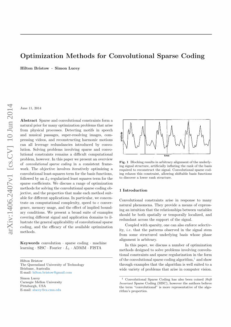
Fig. 2 A brief history of the works that influenced the direction of the convolutional sparse coding problem, and how it isoptimized. The text within each box indicates the theme or idea that the paper introduced.

patches (Sohn and Jung, 2011) and unsupervised learn-

ing of hierarchical generative models (Lee et al., 2009;

Zeiler et al., 2010).

The large-scale nature of the latter applications

have placed great demands on the computational ef-

ficiency of the underlying algorithms. Coupled with

the steady advances in machine learning and comput-

ing, this has given rise to a range of optimization ap-

proaches for convolutional sparse coding. (Chalasani

and Principe, 2012) introduced a convolutional exten-

sion to the FISTA algorithm for sparse inference (Beck

and Teboulle, 2009), and (Bristow et al., 2013) intro-

duced a Fourier method based on the closely-related

ADMM (Boyd, 2010). Convolutional basis learning

has largely been relegated to gradient descent, how-

ever (Grosse et al., 2007) introduced a Fourier domain

adaptation that minimized the inequality constrained

problem via the Lagrange dual.

In this paper, we make the following contributions:

1. We provide a brief discussion detailing the works

that influenced the development of the convolu-

tional sparse coding algorithm and how it stems

from natural processes.

2. We argue that convolutional sparse coding makes

a set of assumptions that are more appropriate in

many tasks where block or sampled sparse coding is

currently used.

3. We discuss practical optimization of convolutional

sparse coding, including speed, memory usage and

assumptions on boundary conditions.

4. We show through a number of examples the applica-

bility of convolutional sparse coding to a wide range

of problems that arise in computer vision, and when

particular problems benefit from different optimiza-

tion methods.

It is worth emphasising that the algorithms presented in

this work are not new. Detailed treatments of the algo-

rithms can be found in their respective works (Bristow

et al., 2013; Chalasani and Principe, 2012; Grosse et al.,

2007). Rather, this paper aims to present the available

algorithms in a unified framework and act as a resource

for practitioners wishing to understand their properties.

4 Hilton Bristow, Simon Lucey

f(x)

✏

min f(x)

s.t. ||x||2 ✏

min f(x)

s.t. |x|1 ✏

x⇤u x⇤

u

x⇤c x⇤

c

(b)

(a)

- Laplacian- Cauchy- Gaussian

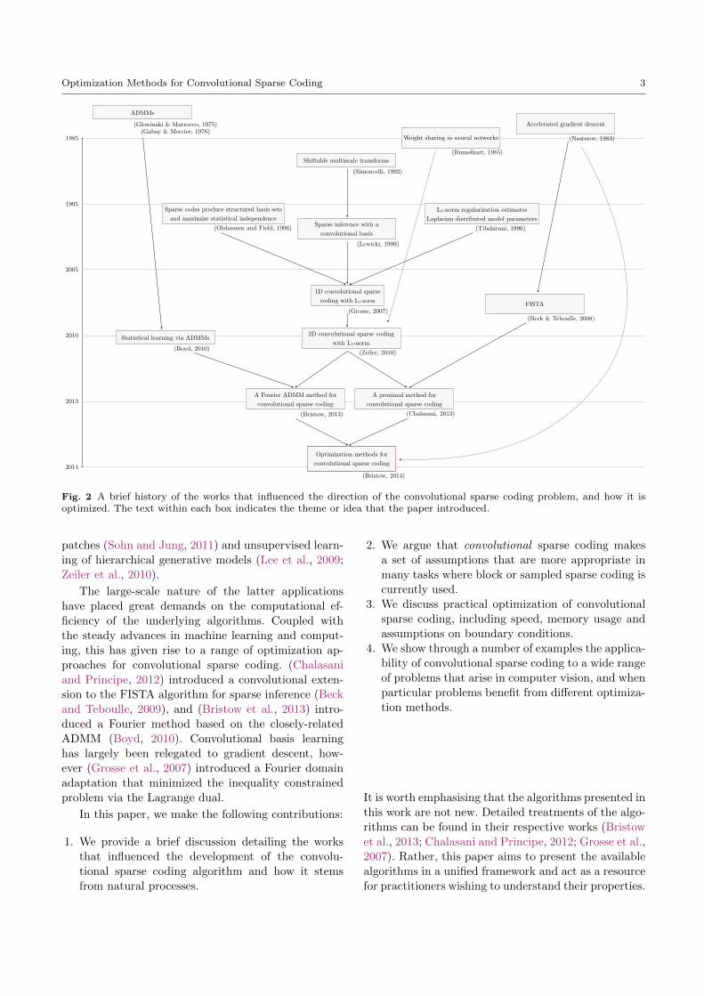
Fig. 3 Sparsifying distributions and their effect as regulariz-ers. (a) For a given variance, the Laplacian and Cauchy dis-tributions have more probability mass centered around zero.(b) As a result, L1 constraints favour axis-aligned solutions(only the second dimension is non-zero).

1.1 Outline

We begin in §2 with an introduction of the convolu-

tional sparse coding formulation. We discuss optimiza-

tion methods for convolutional sparse inference first in

§3, as they are of most algorithmic interest, followed by

methods for basis/filter updates in §4. In §6 we present

a number of applications of convolutional sparse cod-

ing, each with a discussion of the preferred optimization

method and implication of boundary effects. Proofs and

implementation details are deferred until the appen-

dices.

1.2 Notation

Matrices are written in bold uppercase (e.g . A), vectors

in bold lowercase (e.g . x) and scalars in regular typeface

(e.g . K). Convolution is represented by the ∗ operator,

and correlation by the ? operator. We treat all signals as

vectors - higher-dimensional spatial or spatio-temporal

signals are implicitly vectorized - however operations on

these signals are performed in their original domain. We

adopt this notation because (i) the domain of the signal

is largely irrelevant in our analysis and the algorithms

we present, and (ii) for any linear transform in the orig-

inal domain, there exists an equivalent transform in the

vectorized domain.

A ˆ applied applied to any vector denotes the Dis-

crete Fourier Transform (DFT) of a vectorized signal

a such that a ← F(a) = Fa, where F() is the Fourier

transform operator and F is the D×D matrix of com-

plex Fourier bases.

2 Convolutional Sparse Coding

The convolutional sparse coding problem consists of

minimizing a convolutional model-fitting term f and

a sparse regularizer g,

arg mind,z

f(d, z) + βg(z) (1)

where d is the convolutional kernel, z are the set of

sparse coefficients, and β controls the tradeoff between

reconstruction error and sparsity of representation. The

input can be reconstructed via the convolution,

x = d ∗ z . (2)

Assuming Gaussian distributed noise and Laplacian

distributed coefficients, Eqn. 1 can be written more for-

mally as,

arg mind,z

1

2||x− d ∗ z||22 + β||z||1

s.t. ||d||22 ≤ 1 (3)

The remainder of our analysis is based around effi-

cient methods of optimizing this objective. The objec-

tive naturally extends to multiple images and filters,

arg mind,z

1

2

M∑i=1

||xi −N∑j=1

(dj ∗ zi,j)||22 + β

M∑i=1

N∑j=1

||zi,j ||1

s.t. ||dj ||22 ≤ 1 ∀ j ∈ 1 . . . N (4)

however this form quickly becomes unwieldy, so we only

use it when the number of filters or images needs to be

emphasized.

Contrast the objective of Eqn. 3 with that of con-

ventional sparse coding,

arg minB,Z

||X−BZ||22 + β||Z||1

s.t. ||Bi||22 ≤ 1 ∀ i (5)

Here, we are solving for a set of basis vectors B and

sparse coefficients Z in alternation that reconstruct

patches or samples of the signal X in isolation. This

Optimization Methods for Convolutional Sparse Coding 5

is an important distinction to make, and forms the fun-

damental difference between convolutional and patch-

based sparse coding.

In the limit when X contains every patch from the

full image, the two sparse coding algorithms behave

equivalently, however the patch-based algorithm must

store a redundant amount of data, and cannot take ad-

vantage of fast methods for evaluating the inner prod-

uct of the basis with each patch (i.e. convolution).

The objective of Eqn. 3 is bilinear – solving for each

variable whilst holding the other fixed yields a convex

subproblem, however the objective is not jointly convex

in both. We optimize the objective in alternation, iter-

ating until convergence. There are no guarantees that

the final minima reached is the global minima, however

in practice multiple trials reach minima of comparable

quality, even if the exact bases and distribution of co-

efficients learned are slightly different.

In the sections that follow, we introduce a range

of algorithms that can solve for the filters and coef-

ficients. Since the alternation strategy treats each in-

dependently, we largely consider the algorithms in iso-

lation, however some care must be taken in matching

appropriate boundary condition assumptions.

2.1 Other Formulations

It should be noted that the algorithm of Eqn. 3 is not

the only conceivable formulation of convolutional sparse

coding. In particular, there has been growing interest

in non-convex sparse coding with hyper-Laplacian, L0+

and other exotic priors (Zhang, 2010; Wipf et al., 2011).

Whilst these methods have not yet been extended to

convolutional sparse coding, there is no fundamental

barrier to doing so.

3 Solving for Coefficients

It is natural to begin with methods for convolutional

sparse inference, since this is where most of the research

effort has been focussed. Solving for the coefficients z

involves optimizing the unconstrained objective,

arg minz||x− d ∗ z||22 + β||z||1 (6)

where β controls the tradeoff between sparsity and re-

construction error. This objective is difficult to solve

because (i) it involves a non-smooth regularizer, (ii) the

least-squares system cannot be solved directly (forming

explicit convolutional matrices for large inputs is infea-

sible), and (iii) the system involves a large number of

variables, especially if working with megapixel imagery,

etc.

In the case of multiple images and filters,

arg minz

1

2

M∑i=1

||(xi −

N∑j=1

(dj ∗ zi,j))||22

+ β

M∑i=1

N∑j=1

||zi,j ||1 (7)

and given that the minima of the sum of convex func-

tions is the sum of their minima,

minz

M∑i=1

fi(z) =

M∑i=1

minzfi(z) (8)

the coefficients for each image can be inferred sepa-

rately,

z?i = arg minz

1

2||xi −

N∑j=1

(dj ∗ zi,j)||22 + β

N∑j=1

||zi,j ||1

(9)

The two methods that we introduce are both based

around partitioning the objective into the smooth

model-fitting term and non-smooth regularizer that can

then be handled separately.

3.1 ADMM Partitioning

The alternating direction method of minimizers (ADMM),

was proposed jointly by (Glowinski and Marroco, 1975;

Gabay and Mercier, 1976), though the idea can be

traced back as early as Douglas-Rachford splitting

in the mid-1950s. (Boyd, 2010) presents a thorough

overview of ADMMs and their properties. ADMMs

solve problems of the form,

arg minz,t

g(z) + h(t)

s.t. Az + Bt = c (10)

To express convolutional sparse inference in this

form, we perform the (somewhat unintuitive) substi-

tution,

g(z) =1

2||x− d ∗ z||22 h(z) = β||z||1 (11)

A = I B = −I c = 0 (12)

to obtain,

arg minz,t

1

2||x− d ∗ z||22 + β||t||1

s.t. z = t (13)

By introducing a proxy t, the loss function can be

treated as a sum of functions of two independent vari-

ables, and with the addition of equality constraints, the

6 Hilton Bristow, Simon Lucey

minima of the new constrained objective is the same as

the original unconstrained objective.

Whilst the individual functions may be easier to

optimize, there is added complexity in enforcing the

equality constraints. Taking the Lagrangian of the aug-

mented objective,

L(z, t,λ) = g(z) + h(t) +ρ

2||z− t + λ||22 (14)

the solution is to minimize the primal variables, and

maximize the dual variables,

z?, t?,λ? = arg maxλ

(arg min

z,tL(z, t,λ)

)(15)

Optimizing in alternation (which accounts for the term

alternating direction) yields a strategy for updating the

variables involving a function of a single variable plus

a proximal term binding all variables,

zk+1 = arg minz

g(zk) +ρ

2||zk − (t− λ)||22 (16)

tk+1 = arg mint

h(tk) +ρ

2||tk − (z + λ)||22 (17)

λk+1 = λk + ρ(z− t) (18)

The intuition behind this strategy is to find a set

of model parameters which don’t deviate too far from

the regularization parameters, then visa versa, to find

a set of regularization parameters which are close to

the model parameters. The Lagrange variables impose

a linear descent direction that force the two primal vari-

ables to equality over time.

For this strategy to be effective, the sum of the func-

tion g or h and an isotropic least-squares must be easy

to solve.

Substituting the convolutional sparse inference ob-

jective into Eqn. 16,

zk+1 = arg minz

1

2||x− d ∗ zk||22 +

ρ

2||zk − (t− λ)||22(19)

tk+1 = arg mintβ||tk||1 +

ρ

2||tk − (z + λ)||22 (20)

The z update takes the form of generalized Tikhonov

regularization. In the t update, the L1-regularizer can

now be treated independently of the model-fitting

term, and importantly the added proximal term is an

isotropic Gaussian, so each pixel of t can be updated

independently,

tk+1 = arg mint

β|tk|+ ρ

2(tk − z + λ)2 (21)

the solution to which is the soft thresholding operator,

t? = sgn (z + λ) ·max

{|z + λ| − β

ρ, 0

}(22)

In the ADMM, the minimizer t? is exactly sparse,

whilst the minimizer z? is only close to sparse. If exact

sparsity is a concern in the problem domain, t? should

be retained at the point of convergence.

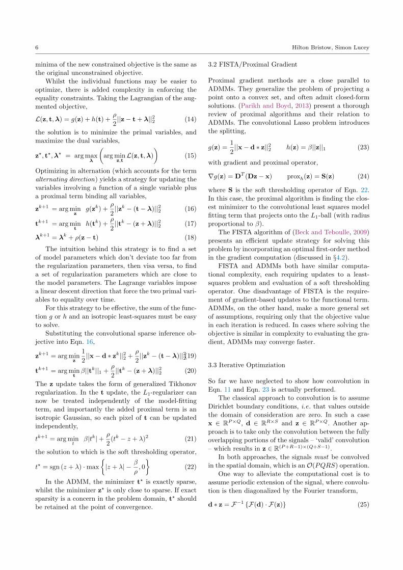
3.2 FISTA/Proximal Gradient

Proximal gradient methods are a close parallel to

ADMMs. They generalize the problem of projecting a

point onto a convex set, and often admit closed-form

solutions. (Parikh and Boyd, 2013) present a thorough

review of proximal algorithms and their relation to

ADMMs. The convolutional Lasso problem introduces

the splitting,

g(z) =1

2||x− d ∗ z||22 h(z) = β||z||1 (23)

with gradient and proximal operator,

∇g(z) = DT (Dz− x) proxh(z) = S(z) (24)

where S is the soft thresholding operator of Eqn. 22.

In this case, the proximal algorithm is finding the clos-

est minimizer to the convolutional least squares model

fitting term that projects onto the L1-ball (with radius

proportional to β).

The FISTA algorithm of (Beck and Teboulle, 2009)

presents an efficient update strategy for solving this

problem by incorporating an optimal first-order method

in the gradient computation (discussed in §4.2).

FISTA and ADMMs both have similar computa-

tional complexity, each requiring updates to a least-

squares problem and evaluation of a soft thresholding

operator. One disadvantage of FISTA is the require-

ment of gradient-based updates to the functional term.

ADMMs, on the other hand, make a more general set

of assumptions, requiring only that the objective value

in each iteration is reduced. In cases where solving the

objective is similar in complexity to evaluating the gra-

dient, ADMMs may converge faster.

3.3 Iterative Optimziation

So far we have neglected to show how convolution in

Eqn. 11 and Eqn. 23 is actually performed.

The classical approach to convolution is to assume

Dirichlet boundary conditions, i.e. that values outside

the domain of consideration are zero. In such a case

x ∈ RP×Q, d ∈ RR×S and z ∈ RP×Q. Another ap-

proach is to take only the convolution between the fully

overlapping portions of the signals – ‘valid’ convolution

– which results in z ∈ R(P+R−1)×(Q+S−1).In both approaches, the signals must be convolved

in the spatial domain, which is an O(PQRS) operation.

One way to alleviate the computational cost is to

assume periodic extension of the signal, where convolu-

tion is then diagonalized by the Fourier transform,

d ∗ z = F−1 {F(d) · F(z)} (25)

Optimization Methods for Convolutional Sparse Coding 7

where d ∈ RP×Q and z ∈ RP×Q (see §4.5 for the correct

method of padding d to size). This method of convolu-

tion has cost O(PQ log(PQ)).

Both ADMMs and FISTA can take advantage of it-

erative methods, by taking accelerated (proximal) gra-

dient steps. In the next section we show how solving the

entire system of equations in the Fourier domain is only

slightly more complex than performing a single gradient

step, and can lead to faster overall convergence of the

ADMM. An important distinction between FISTA and

ADMMs is that FISTA is constrained to use gradient

updates – it cannot take advantage of direct solvers.

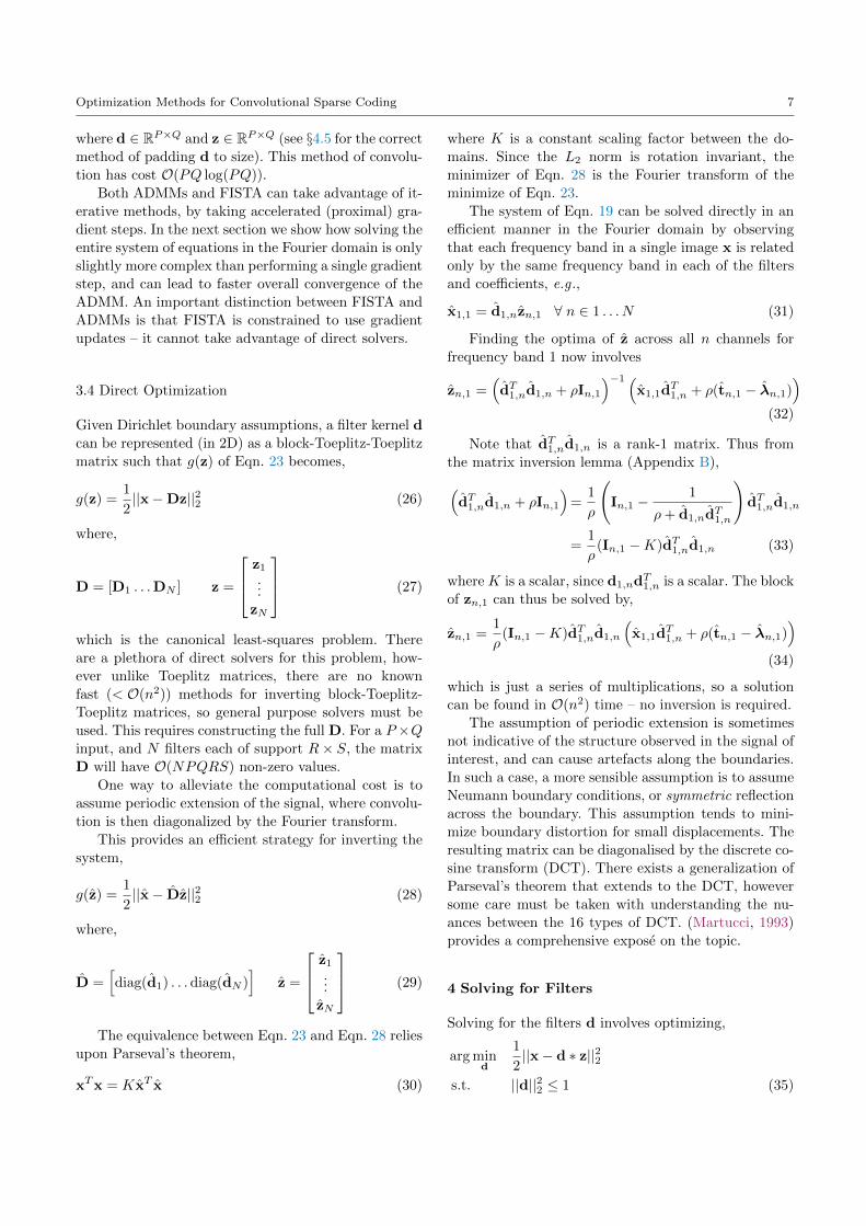
3.4 Direct Optimization

Given Dirichlet boundary assumptions, a filter kernel d

can be represented (in 2D) as a block-Toeplitz-Toeplitz

matrix such that g(z) of Eqn. 23 becomes,

g(z) =1

2||x−Dz||22 (26)

where,

D = [D1 . . .DN ] z =

z1...

zN

(27)

which is the canonical least-squares problem. There

are a plethora of direct solvers for this problem, how-

ever unlike Toeplitz matrices, there are no known

fast (< O(n2)) methods for inverting block-Toeplitz-

Toeplitz matrices, so general purpose solvers must be

used. This requires constructing the full D. For a P ×Qinput, and N filters each of support R× S, the matrix

D will have O(NPQRS) non-zero values.

One way to alleviate the computational cost is to

assume periodic extension of the signal, where convolu-

tion is then diagonalized by the Fourier transform.

This provides an efficient strategy for inverting the

system,

g(z) =1

2||x− Dz||22 (28)

where,

D =[diag(d1) . . . diag(dN )

]z =

z1...

zN

(29)

The equivalence between Eqn. 23 and Eqn. 28 relies

upon Parseval’s theorem,

xTx = KxT x (30)

where K is a constant scaling factor between the do-

mains. Since the L2 norm is rotation invariant, the

minimizer of Eqn. 28 is the Fourier transform of the

minimize of Eqn. 23.

The system of Eqn. 19 can be solved directly in an

efficient manner in the Fourier domain by observing

that each frequency band in a single image x is related

only by the same frequency band in each of the filters

and coefficients, e.g .,

x1,1 = d1,nzn,1 ∀ n ∈ 1 . . . N (31)

Finding the optima of z across all n channels for

frequency band 1 now involves

zn,1 =(dT1,nd1,n + ρIn,1

)−1 (x1,1d

T1,n + ρ(tn,1 − λn,1)

)(32)

Note that dT1,nd1,n is a rank-1 matrix. Thus from

the matrix inversion lemma (Appendix B),(dT1,nd1,n + ρIn,1

)=

1

ρ

(In,1 −

1

ρ+ d1,ndT1,n

)dT1,nd1,n

=1

ρ(In,1 −K)dT1,nd1,n (33)

where K is a scalar, since d1,ndT1,n is a scalar. The block

of zn,1 can thus be solved by,

zn,1 =1

ρ(In,1 −K)dT1,nd1,n

(x1,1d

T1,n + ρ(tn,1 − λn,1)

)(34)

which is just a series of multiplications, so a solution

can be found in O(n2) time – no inversion is required.

The assumption of periodic extension is sometimes

not indicative of the structure observed in the signal of

interest, and can cause artefacts along the boundaries.

In such a case, a more sensible assumption is to assume

Neumann boundary conditions, or symmetric reflection

across the boundary. This assumption tends to mini-

mize boundary distortion for small displacements. The

resulting matrix can be diagonalised by the discrete co-

sine transform (DCT). There exists a generalization of

Parseval’s theorem that extends to the DCT, however

some care must be taken with understanding the nu-

ances between the 16 types of DCT. (Martucci, 1993)

provides a comprehensive expose on the topic.

4 Solving for Filters

Solving for the filters d involves optimizing,

arg mind

1

2||x− d ∗ z||22

s.t. ||d||22 ≤ 1 (35)

8 Hilton Bristow, Simon Lucey

This is a classical least squares objective with norm in-

equality constraints. Norm constraints on the bases are

necessary since there always exists a linear transforma-

tion of d and z which keeps (d ∗ z) unchanged whilst

making z approach zero. Inequality constraints are suf-

ficient since deflation of z will always cause d to lie on

the constraint boundary ||d||22 = 1 (whilst forming a

convex set).

Eqn. 35 is a quadratically constrained quadratic

program (QCQP), which is difficult to optimize in gen-

eral. Each of the following methods relax this form in

one way or another to make it more tractable to solve.

The convolutional form of the least squares term

also poses some challenges for optimization, since (i)

the filter has smaller support than the image it is being

convolved with, and (ii) forming an explicit multiplica-

tion between the filters and a convolutional matrix form

of the images is prohibitively expensive (as per §3.4).

In the case of multiple images and filters,

arg mind

1

2||M∑i=1

(xi −

N∑j=1

(dj ∗ zi,j))||22

s.t. ||dj ||22 ≤ 1 ∀ j ∈ 1 . . . N (36)

one can see that all filters are jointly involved in recon-

structing the inputs, and so must be updated jointly.

4.1 Gradient Descent

The gradient of the objective is given by,

∇fi =

N∑j=1

dj ∗M∑k=1

(zi,j ? zi,k)

− M∑k=1

(xi ? zi,j) (37)

This involves collecting the correlation statistics across

the coefficient maps and images. Since the filters are

of smaller support than the coefficient maps and im-

ages, we collect only “valid” statistics, or regions that

don’t incur boundary effects. In the autocorrelation of

z, one of the arguments must be zero padded to the

appropriate size.

Given the gradient direction, updating the the filters

involves,

dk+1 = dk − t∇f (38)

Computing the step size, t, can be done either via line

search or by solving a 1D optimization problem which

minimizes the reconstruction error in the gradient di-

rection,

arg mint||x−

(dk − t∇f

)︸ ︷︷ ︸dk+1

∗z||22 (39)

the closed-form solution to which is,

t =(x− d ∗ z)T (∇f ∗ z)

(∇f ∗ z)T (∇f ∗ z)(40)

and involves evaluating only 2N convolutions (N if the

x − d ∗ z term has been previously computed as part

of a stopping criteria, etc.). In the case of a large num-

ber of inputs M , stochastic gradient descent is typically

used (Mairal et al., 2009).

Typically after each gradient step, if the new iterate

exists outside the L2 unit ball, the result is projected

back onto the ball. This is not strictly the correct way

to enforce the norm-constraints, however it works with-

out side-effects in practice. The ADMM (§4.3) and La-

grange dual (§4.4) methods on the other hand, both

solve for the norm constraints exactly.

4.2 Nesterov’s Accelerated Gradient Descent

Prolific mathematician Yurii Nesterov introduced an

optimal2 first-order method for solving smooth convex

functions (Nesterov, 1983). Convolutional least squares

objectives require a straightforward application of ac-

celerated proximal gradient (APG).

Without laboring on the details introduced by

Nesterov, the method involves iteratively placing an

isotropic quadratic tangent to the current gradient di-

rection, then shifting the iterate to the minima of the

quadratic. The curvature of the quadratic is computed

by estimating the Lipschitz smoothness of the objec-

tive.

Checking for Lipschitz smoothness feasibility us-

ing backtracking requires two projections per iteration.

This can be costly since each projection involves mul-

tiple convolutions. In practice we find this method no

faster than regular gradient descent with optimal step-

size calculation.

4.3 ADMM Partitioning

As per §3.1, treating convolution in the Fourier domain

can lead to efficient direct optimization. Unlike solving

for the coefficients, however, the learned filters must be

constrained to be small support, and there is no way to

do this explicitly via Fourier convolution.

2 Optimal in the sense that it has a worst-case convergencerate that cannot be improved whilst remaining first-order.

Optimization Methods for Convolutional Sparse Coding 9

An approach to handling this is via ADMMs again,

arg mind,s

1

2||x− Zs||22

s.t. dj = ΦT sj ∀ j ∈ 1 . . . N

||dj ||22 ≤ 1 ∀ j ∈ 1 . . . N (41)

where,

x =

x1

...

xM

d =

d1

...

dN

Z =

diag(z1,1) . . . diag(z1,N )...

. . .

diag(zM,1) diag(zM,N )

(42)

and Φ is a submatrix of the Fourier matrix that corre-

sponds to a small spatial support transform.

Intuitively, we are trying to learn a set of filters s

that minimize reconstruction error in the Fourier do-

main and are small support in the spatial domain.

Taking the augmented Lagrangian of the objective

and optimizing over d and s in alternation yields the

update strategy,

sk+1 = arg mins||x− Zsk||22 +

ρ

2||sk − (Φd− λ)||22 (43)

dk+1= arg mind||Φdk − (s + λ)||22

s.t. ||dj ||22 ≤ 1 ∀ j ∈ 1 . . . N (44)

λk+1= λk + ρ(Φd− s) (45)

In a similar fashion to Eqn. 32, each frequency com-

ponent in s jointly across all filters can be solved for in-

dependently via a variable reordering to produce P ×Qdense systems of equations.

Solving for d appears more involved, however the

unconstrained loss function can be minimized in closed-

form,

d? = dTΦTΦd− 2dTΦT (s− λ) + c

= ΦT (s− λ) (46)

since Φ is an orthonormal matrix, and thus ΦTΦ = I.

Further, the matrix multiplication can instead be re-

placed by the inverse Fourier transform, followed by a

selection operator M which keeps only the small sup-

port region,

d? =M(F−1{s− λ}

)(47)

Handling the inequality constraints is now trivial.

Since Φ is orthonormal (implying an isotropic regres-

sion problem), projecting the optimal solution to the

unconstrained problem onto the L2 ball,

d? =

{||d?k||−22 d?k, if ||d?k||22 ≥ 1

d?k, otherwise(48)

is equivalent to solving the constrained problem.

4.4 Lagrange Dual

Rather than using gradient descent with iterative pro-

jection, Eqn. 35 can be solved by taking the Lagrange

dual in the Fourier domain,

L(d, λ) = ||x− Zd||22 + dTΛd− 1Tλ (49)

where λ ≥ 0 are the dual variables, and Λ = diag(λ).

Finding the optimum involves minimizing the primal

variables, and maximizing the dual variables,

d?, λ?

= arg maxλ

(arg min

dL(d, λ)

)(50)

The closed-form solution to the primal variables is,

d? = (ZT Z + Λ)−1(ZT x) (51)

Substituting this expression for d into the Lagrangian,

we analytically derive the dual optimization problem.

4.5 Convolving with Small Support Filters in the

Fourier Domain

In order to convolve two signals in the Fourier domain,

their lengths must commute. This involves padding the

shorter signal to the length of the longer. Some care

must be taken to avoid introducing phase shifts into

the response, however. Given a 2D filter z ∈ RP,Q, we

can partition it into 4 blocks,

z =

∣∣∣∣z1,1 z1,2z2,1 z2,2

∣∣∣∣ (52)

where, in the case of odd-sized filters, the blocks are

partitioned above and to the left of the central point.

Given a 2D image x ∈ RM,N , the padded representation

z? ∈ RM,N can thus be formed as,

z =

∣∣∣∣∣∣∣∣∣∣∣∣

z2,2 z2,1. . .

. . . 0 . . .. . .

z1,2 z1,1

∣∣∣∣∣∣∣∣∣∣∣∣(53)

This transform is illustrated in Fig. 4. For a comprehen-

sive guide to Fourier domain transforms and identities,

including appropriate handling of boundary effects and

padding, see (Oppenheim et al., 1996).

10 Hilton Bristow, Simon Lucey

1 243

4

1

3

2

⇤ �= F{ } F{ }

. . .

. . . 0 . . .. . .

}}F�1

Fig. 4 Swapping quadrants and padding the filter to the sizeof the image permits convolution in the Fourier Domain

5 Stopping Criteria

For the gradient-based algorithms – gradient descent,

APG and FISTA – a sufficient stopping criteria is to

threshold the residual between two iterates,

||xk+1 − xk||22 ≤ ε (54)

where x is the variable being minimized.

Estimating convergence of the ADMM-based meth-

ods is more involved, including deviation from primal

feasibility,

||d− s||22 ≤ ε , ||z− t||22 ≤ ε (55)

and dual feasibility,

||λk+1 − λk||22 ≤ ε (56)

However, in practice it is usually sufficient to measure

only primal feasibility, since if the iterates have reached

primal feasibility, dual feasibility is unlikely to improve

(this is doubly true when using a strategy for increasing

ρ).

6 Applications

6.1 Example 1 - Image and Video Compression

Many image and video coding algorithms such as

JPEG (Wallace, 1991) and H.264 (Sullivan, 2004) dis-

cretize each image into blocks which are transformed,

quantized and coded independently.

Using convolutional sparse coding, an entire image x

can be coded onto a basis d with sparse reconstruction

coefficients z. Quality and size can be controlled via

the β parameter. The basis can either be specific to the

image, or a generic basis (such as Gabor) which is part

of the coding spec and need not be transferred with the

image data.

Since the coefficients of z are exactly sparse by

virtue of the soft-thresholding operator, the representa-

tion can make effective use of run-length and Huffman

entropy coding techniques. 3

3 JPEG also uses run-length coding but its efficiency is afunction of the quantization artefacts.

To reconstruct the image xr, the decoder simply

convolves the bases with the transmitted coefficients,

xr =

N∑j=1

dj ∗ zj (57)

This matches the media model well: media is consumed

more frequently than it is created, so encoding can be

costly (in this case an inverse inference problem) but

decoding should be fast – convolutional primitives are

hardware-accelerated on almost all modern chipsets.

6.2 Example 2 - A basis for Natural Images

The receptive fields of simple cells in the mammalian

primary visual cortex can be characterized as being spa-

tially localized, oriented and bandpass. (Olshausen and

Field, 1996) hypothesized that such fields could arise

spontaneously in an unsupervised strategy for maxi-

mizing the sparsity of the representation. Sparsity can

be interpreted biologically as a metabolic constraint -

firing only a few neurons in response to a stimulus is

clearly more energy efficient than firing a large number.

(Olshausen and Field, 1996) use traditional patch-

based sparse coding to solve for a set of basis functions.

The famous result is that the basis functions resem-

ble Gabor filters. However, a large number of the bases

learned are translations of others – an artefact of sam-

pling and treating each image patch independently.

It is well-understood that the statistics of natu-

ral images are translation invariant (Hyvarinen et al.,

2009), i.e. the covariance of natural images depends

only on the distance,

Σ (I(x, y), I(x′, y′)) = f((x− x′)2 + (y − y′)2

)(58)

Thus it makes sense to code natural images in a manner

that does not depend on exact position of the stimulus.

Convolutional sparse coding permits this, and as a re-

sult produces a more varied range of basis elements than

simple Gabor filters when coding natural images. The

sparsity pattern of convolutional coefficients also has a

mapping onto the receptive fields of active neurons in

V1.4

6.3 Example 3 - Structure from Motion

Trajectory basis Non-Rigid Structure from Motion

(NRSfM) refers to the process of reconstructing the mo-

4 Unlike many higher regions within the visual cortex, V1is retinotopic – the spatial location of stimulus in the visualworld is highly correlated with the spatial location of activeneurons within V1.

Optimization Methods for Convolutional Sparse Coding 11

tion of 3D points of a non-rigid object from only their

2D projected trajectories.

Reconstruction relies on two inherently conflicting

factors: (i) the condition of the composed camera and

trajectory basis matrix, and (ii) whether the trajectory

basis has enough degrees of freedom to model the 3D

point trajectory. Typically, (i) is improved with a low-

rank basis, and (ii) is improved with a higher-rank ba-

sis.

The Discrete Cosine Transform (DCT) basis has

traditionally been used as a generic basis for encoding

motion trajectories, however choosing the correct rank

has been a difficult problem. (Zhu and Lucey, 2014) pro-

posed the use of convolutional sparse coding to learn a

compact basis that could model the trajectories taken

from a corpus of training data.

Learning the basis proceeds as per usual,

arg mind,z

1

2

M∑i=1

||(xi −

N∑j=1

(dj ∗ zi,j))||22

+ β

M∑i=1

N∑j=1

||zi,j ||1

s.t. ||dj ||22 ≤ 1 ∀ j ∈ 1 . . . N (59)

where each xi is a 1D trajectory of arbitrary length,

d the trajectory basis being learned, and z the sparse

reconstruction coefficients.

Given the convolutional trajectory basis d, recon-

structing the sparse coefficients for the 3D trajectory

from 2D observations involves,

z∗ = arg minz||z||1

s.t. Qx︸︷︷︸u

= Q

N∑j=1

dj ∗ zj (60)

where u are the 2D observations of the 3D points x

that have been imaged by the camera matrices Q, one

for each frame in the trajectory,

Q =

Q1

. . .

QF

(61)

In single view reconstruction, back-projection is typ-

ically enforced as a constraint, and the objective is to

minimize the number of non-zero coefficients in the re-

constructed 3D trajectory that satisfy this constraint.

A convolutional sparse coded basis produces less 3D

reconstruction error than previously explored bases, in-

cluding one learned from patch-based sparse coding,

and a generic DCT basis. This illustrates convolutional

sparse coding’s ability to learn low rank structure from

misaligned trajectories stemming from the same under-

lying dynamics (e.g . articulated human motion).

6.4 Example 4 - Mid-level Generative Parts

Zeiler et al . show how a cascade of convolutional sparse

coders can be used to build robust, unsupervised mid-

level representations, beyond the edge primitives of

§6.2.

The convolutional sparse coder at each level of the

hierarchy can be defined as,

Cl(dl, zl) =

1

2

M∑i=1

|| fs(zl−1i )︸ ︷︷ ︸xi

−M∑j=1

(dlj ∗ zli,j)||22

+ β

M∑i=1

N∑j=1

||zli,j ||1 (62)

where the extra superscripts on each element indicate

the layer to which they are native.

The inputs x to each layer are the sparse coefficients

of the previous layer, zl−1 after being passed through a

pooling/subsampling operation fs(·). For the first layer,

zl−1 = x, i.e. the input image.

The idea behind this coding strategy is that struc-

ture within the signal is progressively gathered at

a higher and higher level, initially with edge primi-

tives, then mergers between these primitives into line-

segments, and eventually into recurrent object parts.

Layers of convolutional sparse coders have also been

used to produce high quality latent representations

for convolutional neural networks (Lee et al., 2009;

Kavukcuoglu et al., 2010; Chen et al., 2013), though

fully-supervised back-propagation across layers has be-

come popular more recently (Krizhevsky et al., 2012).

6.5 Example 5 - Single Image Super-Resolution

Single-Image Super Resolution (SISR) is the process

of reconstructing a high-resolution image from an ob-

served low-resolution image. SISR can be cast as the

inverse problem,

y = DBx (63)

where x is the latent high-resolution image that we wish

to recover, B is an anti-aliasing filter, D is a downsam-

pling matrix and y is the observed low-resolution image.

The system is underdetermined, so there exist infinitely

many solutions to x. A strategy for performing SISR is

12 Hilton Bristow, Simon Lucey

via a straightforward convolutional extension of (Yang

et al., 2010),

arg mindL,dH ,z

M∑i=1

||DBxi −N∑j=1

(dL,j ∗Dzi,j)||22

+ ||xi −N∑j=1

(dH,j ∗ zi,j)||22

+ β

M∑i=1

M∑j=1

||zi,j ||1

s.t. ||dL,j ||22 ≤ 1 ∀ j ∈ 1 . . .M

||dH,j ||22 ≤ 1 ∀ j ∈ 1 . . .M (64)

where xi and DBxi are a high-resolution and derived

low-resolution training pair, D is the downsampling fil-

ter as before and z are a common set of coefficients

that tie the two representations together. The dictio-

naries dL and dH learn a mapping between low- and

high-resolution image features.

Given a new low-resolution input image xL, the

sparse coefficients are first inferred with respect to the

low-resolution basis,

z? = arg minz||xL −

N∑j=1

(dL,j ∗Dzj)||22 + β||z||1 (65)

and then convolved with the high-resolution basis to

reconstruct the high-resolution image,

xH =

N∑j=1

(dH,j ∗ zj) (66)

6.6 Example 6 - Visualizing Object Detection Features

(Vondrick et al., 2013) presented a method for visual-

izing HOG features via the inverse mapping,

φ−1(y) = arg minx||φ(x)− y||22 (67)

where x is the image to recover, and y = φ(x) is the

mapping of the image into HOG space. Direct opti-

mization of this objective is difficult, since it is highly

nonlinear through the HOG operator φ(), i.e. multiple

distinct images can map to the same HOG representa-

tion.

One possible approach to approximating this objec-

tive is through paired dictionary learning, in a similar

manner to §6.5.

Given an image x and its representation y = φ(x)

in the HOG domain, we wish to find two basis sets, dI

in the image domain and dφ in the HOG domain, and a

common set of sparse reconstruction coefficients z, such

that,

x =

N∑j=1

(dI,j ∗ zj) y =

N∑j=1

(dφ,j ∗ zj) (68)

Intuitively, the common reconstruction coefficients force

the basis sets to represent the same appearance infor-

mation albeit in different domains. The basis pairs thus

provide a mapping between the domains.

Optimizing this objective is a straightforward exten-

sion of the patch based sparse coding used by (Vondrick

et al., 2013),

arg mindI,dφ,z

M∑i=1

||xi −N∑j=1

(dI,j ∗ zi,j)||22

+ ||φ(xi)−N∑j=1

(dφ,j ∗ zi,j)||22

+ β

M∑i=1

M∑j=1

||zi,j ||1

s.t. ||dI,j ||22 ≤ 1 ∀ j ∈ 1 . . .M

||dφ,j ||22 ≤ 1 ∀ j ∈ 1 . . .M (69)

Because we are optimizing over entire images rather

than independently sampled patches, the bases learned

will (i) produce a more unique mapping between pixel

features and HOG features (since translations of fea-

tures are not represented), and (ii) be more expressive

for any given basis set size as a direct result of (i).

Image-scale optimization also reduces blocking arte-

facts in the image reconstructions, leading to more

faithful/plausible representations, with potentially finer-

grained detail.

References

Amir Beck and Marc Teboulle. A Fast Iterative

Shrinkage-Thresholding Algorithm for Linear Inverse

Problems. SIAM Journal on Imaging Sciences, 2(1):

183–202, 2009. 3, 6

Stephen Boyd. Distributed Optimization and Statisti-

cal Learning via the Alternating Direction Method

of Multipliers. Foundations and Trends in Machine

Learning, 3(1):1–122, 2010. 3, 5

Hilton Bristow, Anders Eriksson, and Simon Lucey.

Fast Convolutional Sparse Coding. Computer Vision

and Pattern Recognition (CVPR), 1(2), 2013. 3

Rakesh Chalasani and JC Principe. A fast proxi-

mal method for convolutional sparse coding. In-

ternational Joint Conference on Neural Networks

(IJCNN), 2012. 3

Optimization Methods for Convolutional Sparse Coding 13

B Chen, Gungor Polatkan, Guillermo Sapiro, and David

Blei. Deep Learning with Hierarchical Convolutional

Factor Analysis. Pattern Analysis and Machine In-

telligence (PAMI), pages 1–30, 2013. 11

D Gabay and B Mercier. A Dual Algorithm for the So-

lution of Nonlinear Variational Problems via Finite

Element Approximations. Computers and Mathemat-

ics with Applications, 1976. 5

R Glowinski and A Marroco. Sur L’Approximation,

par Elements Finis d’Ordre Un, et la Resolution,

par Penalisation-Dualite, d’une Classe de Prob-

lemes de Dirichlet non Lineares. Revue Francaise

d’Automatique, 1975. 5

Roger Grosse, Rajat Raina, Helen Kwong, and An-

drew Y Ng. Shift-invariant sparse coding for audio

classification. UAI, 2007. 2, 3

Aapo Hyvarinen, Jarmo Hurri, and Patrik O. Hoyer.

Natural Image Statistics A probabilistic approach to

early computational vision. Computational Imaging

and Vision, 39, 2009. 10

Koray Kavukcuoglu, Pierre Sermanet, Y-lan Boureau,

K. Gregor, M. Mathieu, and Y. LeCun. Learning con-

volutional feature hierarchies for visual recognition.

Advances in Neural Information Processing Systems

(NIPS), (1):1–9, 2010. 2, 11

Alex Krizhevsky, I Sutskever, and G Hinton. Ima-

genet classification with deep convolutional neural

networks. Advances in Neural Information Process-

ing Systems (NIPS), pages 1–9, 2012. 11

Honglak Lee, A. Battle, R. Raina, and A.Y. Ng. Effi-

cient sparse coding algorithms. Advances in Neural

Information Processing Systems, 19:801, 2007. 2

Honglak Lee, Roger Grosse, Rajesh Ranganath, and

Andrew Y. Ng. Convolutional deep belief networks

for scalable unsupervised learning of hierarchical rep-

resentations. International Conference on Machine

Learning (ICML), pages 1–8, 2009. 3, 11

MS Lewicki and TJ Sejnowski. Coding time-varying

signals using sparse, shift-invariant representations.

NIPS, 1999. 2

Julien Mairal, Francis Bach, and J Ponce. Online dic-

tionary learning for sparse coding. Conference on

Machine Learning, 2009. 8

SA Martucci. Symmetric convolution and the discrete

sine and cosine transforms: Principles and applica-

tions. PhD thesis, Georgia Institute of Technology,

1993. 7

Morten Mø rup, Mikkel N Schmidt, and Lars Kai

Hansen. Shift invariant sparse coding of image and

music data. Journal of Machine Learning, pages 1–

14, 2008. 2

Y Nesterov. A method of solving a convex program-

ming problem with convergence rate O(1/kˆ2). So-

viet Mathematics Doklady, 1983. 8

B.A. Olshausen and D.J. Field. Emergence of simple-

cell receptive field properties by learning a sparse

code for natural images. Nature, 381(6583):607–609,

1996. 2, 10

Bruno A Olshausen and David J Field. Sparse Cod-

ing with an Overcomplete Basis Set: A Strategy Em-

ployed by V1? Science, 37(23):3311–3325, 1997. 2

Alan V Oppenheim, Alan S Willsky, and with S. Hamid.

Signals and Systems (2nd Edition). Prentice Hall,

1996. 9

Neal Parikh and Stephen Boyd. Proximal Algorithms.

1(3):1–108, 2013. 6

Eero Simoncelli, William Freeman, Edward Adelson,

and David Heeger. Shiftable multiscale transforms.

Information Theory, 1992. 2

K Sohn and DY Jung. Efficient learning of sparse,

distributed, convolutional feature representations for

object recognition. International Conference on

Computer Vision (ICCV), 2011. 3

GJ Sullivan. The H. 264/AVC advanced video coding

standard: Overview and introduction to the fidelity

range extensions. In Conference on Applications of

Digital Image Processing, pages 1–22, 2004. 10

R Tibshirani. Regression shrinkage and selection via

the lasso. Journal of the Royal Statistical Society, 58

(1):267–288, 1996. 2

Carl Vondrick, Aditya Khosla, Tomasz Malisiewicz, and

Antonio Torralba. HOGgles: Visualizing Object De-

tection Features. International Conference on Com-

puter Vision (ICCV), 2013. 12

GK Wallace. The JPEG Still Picture Compression

Standard. Communications of the ACM, pages 1–17,

1991. 10

DP Wipf, BD Rao, and Srikantan Nagarajan. Latent

Variable Bayesian Models for Promoting Sparsity. In-

formation Theory, 57(9):6236–6255, 2011. 5

Jianchao Yang, John Wright, Thomas Huang, and

Yi Ma. Image Super-Resolution via Sparse Repre-

sentation. IEEE Transactions on Image Processing,

19(11):1–13, November 2010. 12

MD Zeiler, Dilip Krishnan, and GW Taylor. Decon-

volutional networks. Computer Vision and Pattern

Recognition (CVPR), 2010. 2, 3

Cun-Hui Zhang. Nearly unbiased variable selection un-

der minimax concave penalty. The Annals of Statis-

tics (arXiv), 38(2):894–942, April 2010. 5

Yingying Zhu and Simon Lucey. Convolutional Sparse

Coded Filters Nonrigid Structure From Motion. Pat-

tern Analysis and Machine Intelligence (PAMI),

2014. 2, 11

14 Hilton Bristow, Simon Lucey

A Log Likelihood Interpretation

Minimizing the sparse convolutional objective has an equiv-alent maximum likelihood interpretation,

z? = arg maxz

P (z|x,d)

= arg maxx

P (x|d, z)P (z) (70)

Replacing the product of two probability distributions withthe log of their sums, and negating the expression yields,

z? = arg minz− log(P (x|z,d))− P (z) . (71)

The corresponding unbiased estimators are,

− log(P (x|z,d)) ∝1

2σ2||x− d ∗ z||22 (72)

− log(P (z)) ∝1

2b||z||1 (73)

After choosing appropriate values for the noise variance,

z? = arg minz

1

2||x− d ∗ z||22 + β||z||1 (74)

B Inversion of a Rank-1 + Scaled Identity

Matrix

The Woodbury matrix identity (matrix inversion lemma)states,

(A+ UCV )−1 = A−1 −A−1U(C−1 + V A−1U)−1V A−1 (75)

Substituting A = ρI, C = 1 and U = xT , V = x, where xis a rank-1 column matrix gives,

(ρI + xxT )−1 = (ρI)−1 − (ρI)−1x(1−1

+ xT (ρI)−1x)−1xT (ρI)−1

= (ρI)−1 − (ρI)−1x(1 +1

ρxT x)−1xT (ρI)−1

= (ρI)−1 − (ρI)−1x(ρ+ xT x)−1xT

=1

ρ

(I −

1

ρ+ xT x

)xxT (76)