Optimization in Microeconomics - University Readers · 2 Optimization in Microeconomics Tab le...

Sneak Preview

Optimization in MicroeconomicsBy Christopher Curran & Skip Garibaldi

Included in this preview:

• Copyright Page• Table of Contents• Excerpt of Chapter 1

For additional information on adopting thisbook for your class, please contact us at 800.200.3908 x501 or via e-mail at [email protected]

Custom Publishing Evolved.

Optimization in Microeconomics

By Christopher Curranand Skip Garibaldi

Copyright © 2011 University Readers Inc. All rights reserved. No part of this publication may be reprinted, reproduced, transmitted, or utilized in any form or by any electronic, mechanical, or other means, now known or hereafter invented, including photocopying, microfi lming, and recording, or in any information retrieval system without the written permission of University Readers, Inc.

First published in the United States of America in 2010 by Cognella, a division of University Readers, Inc.

Trademark Notice: Product or corporate names may be trademarks or registered trademarks, and are used only for identifi cation and explanation without intent to infringe.

14 13 12 11 10 1 2 3 4 5

Printed in the United States of America

ISBN: 978-1-60927-735-2

Preface v

Preface

Th is text is the product of teaching a course on mathematical economics for almost 35 years. Th roughout the time that this course has been taught we have maintained the position that a course in mathematical economics is an opportunity to examine how two disciplines analyze an issue—optimization. In their models economists generally assume that some agent is either maximizing or minimizing some function in order to attain an objec-tive. Economists use the mathematics of optimization to derive implications of the models in order to set up ways to test these models. Indeed, the testable implications of the models are what makes this sort of economic theory scientifi c: to be useful, an economic model must yield some implications that are potentially testable. By “testable” we mean that there exist potential outcomes to an economic experiment that would contradict the model. Th is is the approach that informs every part of this text.

Th e textbook describes in detail the mathematical tools necessary to analyze the optimization models used by economists. We move from the simple model of unconstrained optimization with one control variable through unconstrained optimization with multiple control variables to optimization models with equality constraints. In each case we develop all the tools needed to derive the comparative static implications of the model. Moreover, we emphasize the importance of the Envelope Th eorem throughout the text. We end with a discussion of duality theory.

Th e main material of this book is contained in the even-numbered chapters, 2, 4, 6, and 8. Th e odd-numbered chapters 1 and 3 review the mathematics needed in the even chapters, whereas chapters 5 and 7 extend the mathematics used in the even chapters. In the review chapters, we present only the material needed in the subsequent chapters or that we have found our undergraduates to have not remembered from earlier mathematics classes. Th us, unlike many other mathematical economics texts, we do not present encyclopedic discussions of topics like matrix algebra. Th e chapters cover the minimum mathematics necessary for later material.

We believe that the key material in this textbook are the problems included in the various exercise sets. Many of these problems begin with a verbal description of a model that the student has to translate into a mathematical form that he or she can use optimization theory to analyze. Th en the student is asked to translate the results of their mathematical analysis in to words that a non-mathematician can understand. Our students have found these problems to be the main way that they learn the material. Th e exercises are so indispensable to the learning process that we have had our students present their answers in class. While this is a time-consuming process, it has proved to have the additional benefi t of providing the students with an opportunity to improve their communication skills.

vi Preface

We end this brief introduction with a brief note about the numbering convention used in this text. Th e system we use, while intended to making fi nding numbered material in the text easier to locate, may not be familiar to economics students, so it is worth taking a moment to explain it. All of the chapters and their sections are identifi ed with Arabic numbers, e.g., section 7 of chapter 4, etc. We identify all examples, fi gures, tables, theorems, lemmas, and propositions sequentially. Th us, Figure 2.5.1 is the fi rst item in Chapter 2, section 5. If the next item is an example, it will have the label Example 2.5.2. Th is numbering system should make it easier to fi nd these items when they are referenced in the text. Th e numbered equations follow a similar rule, except that all equation numbers are in parentheses. Exercises have their own, albeit similar, numbering system. Exercise 3.3.5 is the fi fth exercise in the third section of Chapter 3.

We end this brief introduction with a few acknowledgements and thanks. First, we acknowledge the silent contributions of David Ford of the Emory Mathematics Department (now retired) to the development of this book. Professor Ford co-taught the Mathematical Economics course with Dr. Curran for over thirty years and during that time patiently corrected his many misunderstandings of the subtleties of mathematical reasoning. Second, it is often said that teaching is the best way to learn a subject. Th is adage certainly is true for us. Th us, we would also like to acknowledge our debt to the many mathematical economics students we have taught. Finally, we would like to thank our wives, Nannette and Julia, for their unwavering support while we completed this project.

Christopher Curran & Skip GaribaldiEmory UniversityAtlanta, Georgia

Memories of Calculus 1

Chapter 1

Memories of Calculus

T o follow along with this book, you will need to use some of the things you learned in calculus. Some things we will recall along the way, but some are too tangential. Th e purpose of this chapter is to recall the latter material.

1.1 FUNCTIONS OF ONE VARIABLE: POSITIVE, INCREASING, CONVEX/CONCAVE UP

Examine the graph of a function f (x) given in Figure 1.1.1. Th e function has the properties listed in Table 1.1.2.

Fi gure 1.1.1 Graph of a function f(x).

2 Optimization in Microeconomics

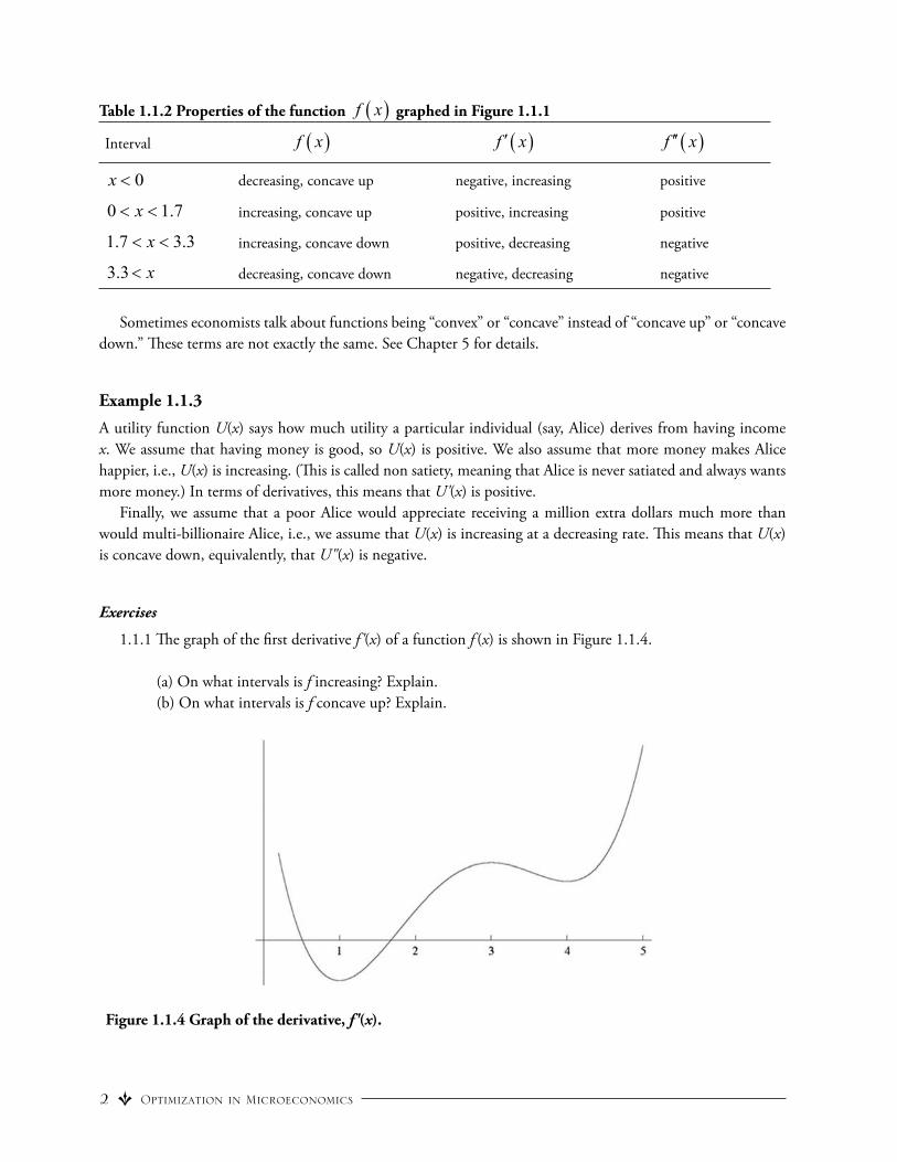
Tab le 1.1.2 Properties of the function f x graphed in Figure 1.1.1

Interval f x f x f x

0x decreasing, concave up negative, increasing positive

0 x 1.7 increasing, concave up positive, increasing positive

1.7 x 3.3 increasing, concave down positive, decreasing negative

3.3 x decreasing, concave down negative, decreasing negative

Sometimes economists talk about functions being “convex” or “concave” instead of “concave up” or “concave down.” Th ese terms are not exactly the same. See Chapter 5 for details.

Ex ample 1.1.3

A utility function U(x) says how much utility a particular individual (say, Alice) derives from having income x. We assume that having money is good, so U(x) is positive. We also assume that more money makes Alice happier, i.e., U(x) is increasing. (Th is is called non satiety, meaning that Alice is never satiated and always wants more money.) In terms of derivatives, this means that U'(x) is positive.

Finally, we assume that a poor Alice would appreciate receiving a million extra dollars much more than would multi-billionaire Alice, i.e., we assume that U(x) is increasing at a decreasing rate. Th is means that U(x) is concave down, equivalently, that U"(x) is negative.

Exercises

1.1.1 Th e graph of the fi rst derivative f '(x) of a function f (x) is shown in Figure 1.1.4.

(a) On what intervals is f increasing? Explain. (b) On what intervals is f concave up? Explain.

Figure 1.1.4 Graph of the derivative, f'(x).


1.2 SECOND-ORDER CONDITIONS

A critical point x* of a function f (x) is a point such that f '(x*)=0. How can you tell if x* is a maximum of f (x)? From calculus, you remember: If f "(x*)<0, then x* is a local maximum, f (x)<– f (x*) that is, f (x)<– f (x*) for x near x*. Th is is known as the second-order condition for a local maximum; if f "(x*)<0, we say that the second-order condition (for x* to be a local maximum) holds. (To remember the second-order condition, it can be helpful to think about parabolas. Th e downward-opening parabola y=–x2 has a maximum

at x = 0 and the second-derivative 2

2 2d ydx is negative. In contrast, the upward-opening

parabola y = x2 has a minimum at x = 0 and the second-derivative 2

2 2d ydx is positive.)

In many cases, we want to know if a critical point x* is a global maximum, that is, if f (x*)>– f (x) for all x. Th e second-order condition for a global maximum is:

Th eorem 1.2.1 (Global SOC Th eore m). Suppose that x* is a critical point for f (x). If f"(x)<0 for all x, then x* is the unique critical point and it is a global maximum for f (x).

Th e theorem makes sense: If f"(x) is always negative, then the graph of the function is concave down, so any local maximum is a global maximum. We give a more rigorous proof for those who want one.

PROOF. For sake of contradiction, suppose that there is another critical point c. Th at is, c ≠ x*and f '(x)=f '(x*)=0. Th en by the Mean Value Th eorem there is some b lying between x* and c such that f"(b)=0. Th is is a contradic-tion, so x* is the unique critical point.

Again, for sake of contradiction, suppose that there is some point e > x* such that f (e) > f (x*). Th en

0 .

f e f xe x

But the Mean Value Th eorem says there is some d such that x* < d < e and

0.d

x

f e f xf d f x dx

e x

Th is is a contradiction, so no such e can exist. An analogous argument shows that there is no e < x* with f (e)>f (x*). Th is shows that x* is a global maximum.

Th is argument also proves the second-order condition for a local maximum that you remember from calculus. In the statement of the theorem, we implicitly assumed that f (x) is defi ned and twice diff erentiable for all

real numbers x, as you can see in the phrase “for all x”. Economists often consider functions f (x) that are only defi ned for positive x; for such a function we could replace “for all x” with “for all positive x”. Such a replace-ment is harmless.*

If we are a little more clever, we can get the same conclusion while assuming less about f (x).Alternate proof of Th eorem 1.2.1 (Global SOC Th eorem). Suppose that we only know the following: If f '(c)=0, then f "(c)<0, i.e., every critical point of f (x) is a local maximum. Obviously this assumption is weaker

* For the mathematically inclined reader: Th e important thing is that we are only considering values of x in some open interval of the x-axis. In the language of economics, we only look for “interior solutions”, and not “corner solutions”.


than the assumption “f "(c)<0 for all x” from the earlier proof of the Global SOC Th eorem. We assume that there is a critical point x* of f (x) and we will show that it is the unique critical point and is a global maximum for f (x).

Because f '(x*)=0 and f "(x*)<0, the derivative f '(x) is positive just left of x* and negative just to the right. If we zoom in on the point (x*, f (x*)) on the graph of f (x), we see what looks like an upside-down parabola with its apex at x*.

For sake of contradiction, suppose there is another critical point c. By our hypothesis on f (x), c is also a local maximum, and when we zoom in on the point (c, f (c)) on the graph of

f (x), we again see an upside-down

parabola. In order to connect these two sections of graph, there must be a point b between c and x* where there is a local minimum. But this is impossible, because every critical point of f (x) is a local maximum. Th erefore, x* is the unique critical point of f (x).

Finally, f (x) < f (x*) for all x x . Otherwise, there is some d such that d x and f d f x .By the Mean Value Th eorem, there is some c properly between d and x* with f c 0 , but this is impossible because x* is the unique critical point.

1.3 CLOSED INTERVALS AND CORNER MAXIMA

So far we have been implicitly assuming that the function f (x) is defi ned on an open interval, say for all x or for all 0.x Th en maxima and minima for such a function will occur at critical points. Th is is the typical situ-ation we fi ll consider in this book.

However, sometimes it is more natural for f (x) to be defi ned on some closed interval, say for a x b .One natural example is when f (x) measures the utility Alice derives from consuming x dollars worth of some good. It is reasonable to imagine that this function may only be defi ned for 0 x I , where I is Alice’s total income. In terms of the story, this would say that Alice can spend nothing on the good, can spend everything she has on the good, or can spend something in between.

In this case, we have a recipe for a solution. First, fi nd all the critical points of f (x) in the interval a x b . Plug these and a and b into f (x). Whichever gives the biggest value is the location of the global maximum. If the maximum is at one of the critical points (lying properly between a and b), we say it is an interior maximum. If the maximum is at one of the endpoints a or b, then we say it is a corner maximum.

Of course, a similar recipe and similar words apply to fi nding a global minimum of the function.

Example 1. 3.1

Let us return to the example where f (x) is Alice’s utility from spending x dollars on some good. As in Example 1.1.3, f '(x) is positive for 0 x I , so there are no critical points. We are left with comparing the value of f (x) at the endpoints 0 and I. As f (x) is increasing and 0,I 0 ,f I f and I is the location of the global maximum for f (x).

Exercises

1.3.1 Look back at the graph of f '(x) in Figure 1.1.2. At what values of x does f have a local maximum? A local minimum? Explain.

1.3.2 Give an example of a function that is defi ned for all x > 0 and such that 1 is a local maximum but not a global maximum. [Th is question has two parts: You have to fi nd such a function, and then you have to explain why the function you found has the desired properties.]


1.3.3 Th e function f (x) = 1n (x) is defi ned for x > 0. Show that f " (x) < 0 and that f (x) has no critical points for. [Th is problem shows why the Global SOC Th eorem starts by assuming that f (x) has a critical point x*. Here we have a function where f " (x) < 0 and there is no global maximum.]

1.3.4 Give an alternative proof of the Global SOC Th eorem using the Fundamental Th eorem of Calculus. [One possible approach is to use the Fundamental Th eorem to show that f ' (x) is positive for x < x* and f ' (x) is negative for x < x* . Th en use the Fundamental Th eorem again to prove the theorem.]

1.3.5 Give an alternative proof of the Global SOC Th eorem using Taylor’s Th eorem. [For a precise statement of Taylor’s Th eorem, see any advanced calculus or real analysis text, such as W. Rudin, Principles of Mathematical Analysis, McGraw-Hill, 1976.]

1.3.6 A man stands on a beach at point A (see Figure 1.3.2) and throws a stick into the water to point D.* His dog, a time-minimizing animal, then fetches the stick by taking one of three routes: (1) swim the whole way to point D, (2) run to point C and swim to point D, or (3) run along the beach to point B and then swim from point B to point D. Th e speed of the dog on the beach is r and the speed of the dog in the water is s.

Figure 1.3.2 What’s the fastest way to the stick?

a. How long will it take the dog to reach point D if he swims the entire way (following route 1)?b. How long will it take the dog to reach point D if he runs to point C and then swims out to point D

(following route 2)?c. How long will it take the dog to reach point D if he runs to point B and then swims to point D (route 3)?d. Looking back at your answer for part (c), if you plug in numbers such that y > z, your formula probably

says something that does not make sense physically. Th at’s okay because we do not care about that case. But why doesn’t your formula from (c) model reality in this case?

e. If r s , what route does the dog take, and why?

* Th is problem is based on T.J. Pennings, Do dogs know calculus?, College Math. Journal, vol. 34 (2003), pp. 178–182.


f. Suppose that r s and2

.

1

x zrs

Find the value y of y that minimizes the time for the dog to

cover route 3. Check the SOC to verify that y is a local minimum. Write y as a function of x and rs .

Verify that y is between 0 and z, i.e., is in the range where your answer for (c) makes sense.

g. Suppose that r s and 2

.

1

x zrs

(Th is is the only case we have not covered yet, and

corresponds to the man throwing the stick much farther into the water than along the beach.) Verify that the derivative of the time t that it takes the dog to run route 3 with respect to y is negative for 0 y z . What route does the dog take in this case?

h. Suppose that you have a particular dog, so that rs is fi xed. Use the results of this problem to describe a

way to test if dogs choose the time-minimizing path to a stick thrown into the water (i.e., to test if dogs are “rational”). Th ere is no single “correct answer to this question since each scientist might design the experiment diff erently. Th ere are descriptions, however, that provide a more thorough description of an experiment that is likely to produce convincing results.

Figure 1.3.3 Graph to accompany Exercise 1.3.6.

1.4 THE CHAIN RULE

Chain rule for functions of one variableIn calculus, you learned the chain rule for functions of one variable:

.d f g x f g x g x

dx

(1.4.1)


Example 1.4.1

If we want to fi nd the derivative of sin x2 1 with respect to x, we can write

2: sin and : 1.f y y y g x x

Th en

sin cos and 2 .df y y y g x xdy

So 2 2sin( 1) 2 cos( 1).d x x xdx

Th e chain rule (1.4.1) can be written diff ere ntly. P ut z : f y and y : g x . Th en*,

, , and g .d dz dz dyf g x f g x xdx dx dy dx

So:

.dz dz dydx dy dx

You used this version of the chain rule many times when you did related rates problems.

Chain rule for functions of several variablesConsider the example:

Example 1.4.2

For 21 2:z x x with 3

1 :x t and 2 : 1,x t we have:

2 212 1 2

2 1 22 1 2

2 2 3 4 3 2

by the product rule,

2 by the chain rule, and

( 1) (3 ) 2 ( 1) 5 8 3 .

dxdz dx x xdt dt dt

dx dxdz x x xdt dt dtdz t t t t t t tdt

Notice that the formula for dzdt has no 1'sx or 2'sx in it. So far, we have just used the chain rule for functions

of one variable. We can re-write this as follows. Suppose that 1 2,z f x x , 1x g t , and x2 h t for some functions f, g, and h. Th en the chain rule says:

1 2

1 2

.dx dxdz z zdt x dt x dt

* Properly speaking, we also have to require that f and g are diff erentiable. But when dealing with economic problems—i.e., everywhere in this course—we assume that all functions appearing are smooth, as explained in the preface. We can do this because all the functions we deal with appear as part of a mathematical model of some real-world situation. Such functions are found by guessing at a formula and making some measurements to fi ll in some parameters. Obviously there is some error in that process. Within your error bounds, you can fi nd a smooth function that adequately approximates the data.

(1.4.2)

(1.4.3)

(1.4.4)


We now re-do Example 1.4.2 We have:

22 1 2

1 2

and 2 .z zx x xx x

So applying equation (1.4.4), we get:

2 1 22 1 22 ,dx dxdz x x x

dt dt dt

and we can fi nish as in Example 1.4.2.We can re-write equation (1.4.4) as:

1 21 2 1 2 1 1 2 2, , , ,x x

d f x x f x x x t f x x x tdt

where 1x

f is shorthand for 1

fx . (Sometimes we will abbreviate this partial derivative still further as

.) Th ere is a useful mnemonic in this re-writing of (1.4.4): for every comma on the left side, there is a plus on the right side.

In a typical economic problem, there is not just one parameter t; there are more. For example, suppose that 1 2,z f x x , where x1 g p,q and x2 h p,q for some functions f , g, and h. Th en,

1 2

1 2

1 2

1 2

.

x xz z zp x p x p

x xz z zq x q x q

Exercises

1.4.1 Using the chain rule (1.4.1) or (1.4.2), fi nd:

(a) 2 sin cos .d x x

dx

(b) 9910001 ( 1) .d x

dx

1.4.2 For z x 3xy y2 and x1 sin(t) and x2 cos(t) , find dzdt using the chain rule (1.4.4).

1.4.3 For 21 1 2z x x x with 1 cosx p q and 2 sin ,x q p find z

p and z

q using the chain

rule 1.4.5.

1.5 EXPONENTIALS AND LOGARITHMS

You remember the Laws of Exponents that you learned in pre-calculus:

, ( ) , and .bb c b c b c bc b c

caa a a a a aa

(1.4.5)

(1.5.1)


You also know how to take a derivative

1 if 0.b bd x bx bdx

Th is is the Power Rule.Th e similar-looking but diff erent derivative d

dxbx requires a diff erent approach. Amongst all positive num-

bers, there is a unique one, e , such that

.x xd e edx

You might remember that e is about* 2.7.

Figure 1.5.1 Graph of .xe

You can see a graph of ex in Figure 1.5.1. Note that the function is increasing, that is, as you move to the right along the x-axis, the value of e x goes up. Th is means that has an inverse function, which we call natural log and denote by ln. Th e statement that ln(x) and are inverse functions means that

ln( )ln( ) for all and for 0.xxx e x e x x

Figure 1.5.2 shows the graph of ln(x).

Figure 1.5.2 Graph of ln(x)

* Careful! e cannot be written as a fi nite decimal or a ratio of two integers; it is a decimal that goes on forever and never settles into a repeating pattern; it is an irrational number. For a proof of this, see Aigner, Ziegler, Proofs from THE BOOK, Springer, 1998.

(1.5.2)


Laws of logarithms

Because In(x) and e x are inverses of each other, the Laws of Exponents (1.5.1) induce similar rules for logarithms:

ln ln ln , ln ln , and ln ln ln .b abc b c a b a a bb

Exponentials, logarithms, and the chain ruleCombining equa tion (1.5.2) with the chain rule (1.4.1) from the previous section gives:

( ) ( ) '( )'( ) and ln ( ) .( )

f x f xd d f xe e f x f xdx dx f x

We can use the fi rst of these rules to evaluate ddx

bx where b is a positive number. We rewrite b as eln(b) , soln( ) ln( ) ln( )( ) ln( ) ln( ).x b x x b x b xd d db e e e b b b

dx dx dx

Th e second rule in (1.5.3) can be rewritten as

'( ) ( ) ln ( ).df x f x f xdx

Th is rule is sometimes known as logarithmic diff erentiation. Applying it to the case where xf x b , we fi nd:

ln( ) ln( ) ln( ).x x x x xd d db b b b x b b bdx dx dx

Th is is the same answer we found before.

Exercises

1.5.1 Use logarithmic diff erentiation to write down a formula for ddx

f (x)g(x ) . Use it to calculate ddx

xx .

1.5.2 Let ( ) 1 (1 )ng n p for some p such that 0 1.p (Perhaps p is a probability.) Calculate '( )g n and ''( )g n and determine their signs for 0.n

1.6 IMPLICIT DIFFERENTIATION

Example 1.6.1

Th e equation for the unit circle is2 2 1.x y

Suppose we want to fi nd a formula for dydx . Th e naive approach is to solve the eq uation for y and then take

the derivative. Th at works great for this example, but will not work for the problems below or anywhere else in this text. So we use another approach: we take the derivative of both sides of the equation with respect to x:

2 2 1d dx ydx dx

(1.5.3)

(1.6.1)


2 2 0 because 1 is a constantd dx ydx dx

2 2 0 using the Chain Ruledx dyx ydx dx

2 2 0 because 1dy dxx ydx dx

2 2dyy xdx

.dy xdx y

Note that both x and y appear on the right side of this equation; that is okay.Th is technique is known as implicit diff erentiation, because of the following reason: Th anks to the Implicit

Function Th eorem (discussed in section 2.7), e quation 1.6.1 implicitly defi nes y as a function of x.

Exercises

1.6.1 Find dydx

by implicit diff erentiation:

(a) 5 2 31 .y x y x y

(b)

cos sin 1.x y

1.7 INEQUALITIES

Rules for inequalities

Let’s remember way back to before calculus, to solving equations involving inequalities. You learned the following fi ve rules:

1. If a b , then .a c b c (“You can add to both sides.”)

2. If a b and ,c d then .a c b d

3. If a b and 0,c then .ac bc (“You can multiply or divide by a positive number.”)

4. If a b and 0,c then .ac bc (“If you multiply or divide by a negative number, you have to fl ip the inequality.”)

5. If 0 ,a b then 1 1 .a b (“If both sides are positive, you can take 1 over each side, but you have to fl ip the inequality.”)


Example 1.7.1

Suppose we want to solve the equation 3 2 8.x Applying Rule 1 with 2,c we can subtract 2 from both sides to get 3 6.x Applying Rule 3 with 1 ,3c we can divide both sides by 3 and fi nd 2.x (For readers who have had a course on mathematical logic, it looks like this argument only shows: “If 3 2 8,x then 2.x ” But Rules 1 through 5 are reversible, so we can do all the steps in the opposite order. Starting with x 2 , we apply Rule 3 with c 3 to get 3 6.x Applying Rule 1 with c 2 gives 3 2 8.x Th is shows that the statements 3x 2 8 and x 2 are equivalent, i.e., 3x 2 8 if and only if x 2 .)

Exponentials and logarithms

We can add two more rules for inequalities:

6. If ,a b then .a be e

7. If 0 ,a b then ln ln .a b

Th ese rules say that the functions ex and ln(x) are increasing. Comparing Rules 6 and 7, Rule 7 has an additional “ 0 a ”; this is just to ensure that ln(a) and ln(b) are defi ned.

Exercises

1.7.1 Let a and b be nonzero numbers. For each of the four possibilities for the signs of a and b, either de-termine the sign of a b or give explicit examples of numbers a and b to show that you cannot deter-mine the sign of .a b

1.7.2 For which values of x do each of the following inequalities hold? Indicate which rule you used at each step of your solution.

(a) 1 3 2 9.x

(b) 5 .x x

(c) 2 5 .x x x

(d) 2 1.x

(e) 2 ln 2 1.x

(f ) ln (3x) > ln (x+2).

1.7.3 Show that ex x 1 for all x 0 . [Hint: Examine : ( 1).xf x e x Obviously f (0) 0. Show that

f '(x) 0 for all x 0.] For which positive numbers b is it true that bx x 1 for all x 0 ?


1.8 ELASTICITY

Recall from intermediate microeconomics the inverse demand function p(q). It tells you the price at which consumers will demand the quantity q of some good. Th e price elasticity of demand

( )p qq

dpdq

measures the relative sensitivity of demand to a change in price.Since p and q are both posit ive, ε has the same sign as p '(q) . For an ordinary good, demand and price move

in opposite directions (the Law of Demand), so p '(q) and ε are both negative. Demand is elastic if ε is less than -1 and is inelastic if ε is between -1 and 0. (A good is called a Giff en good if demand and price move in the same direction, i.e., higher price leads to higher demand. So far, no one has ever presented a clear-cut, well-accepted example of a Giff en good in the real world.)

Given any function f (x) , one can talk about its elasticity, which is defi ned to be

( ).

'( )

f xx

f x

To name this quantity in words, you would say something like “ f elasticity of x”.

Exercises

1.8.1 A monopolist can sell q units of a product at a price p(q) , so that his revenue function is ( ) .R q p q q

(a) Find .R q

(b) Write R q in terms of the price, ,p q and the price elasticity of demand .

(c) Show that marginal revenue R q is positive if demand is elastic, and that R q is negative if demand is inelastic.

(d) Suppose now that that p is a linear function of y. (Th is might be the only type you saw in your microeconomics course.) Show that R q is negative if and only if the good is a normal good.

1.8.2 Th e Cobb-Douglas function 1 2 1 2,f x x Ax x appears often enough in this and other texts that it seems appropriate to mention a few shortcuts that will make computation of the derivatives easier. Th is problem takes you through some of these shortcuts.

(a) Find f1 x1,x2 . [Th e notation 1f is shorthand for

1

fx

. Your calculus book may have used the alter-native shorthand “

1xf ”.]

(b) Show that f1 x1,x2 f x1,x2 x1

.


(c) Show that f11 x1,x2 1 f x1, x2 x1

2.

(d) Calculate f11 x1,x2 f22 x1,x2 f122 x1, x2 in terms of α, β, and f x1,x2 .

(e) Use the answer to (b) to derive an economic interpretation of α assuming that f x1,x2 is output and 1x and 2x are two inputs (that is, assume that f x1,x2 is a production function).

1.9 APPENDIX: REFRESHER ON “IF AND THEN”

“If-then” statements are the foundation of deduction. Consider the statements:If you are from California, then you are from the United States. (1.9.1)

as opposed to:If you are from the United States, then you are from California. (1.9.2)

Th e fi rst statement is true, because California is part of the United States, and the second statement is false be-cause many people are from other places in the US. Th is illustrates the diff erence between the two general forms:

If A, then B. (1.9.3)and its converse

If B, then A. (1.9.4)Comparing (1.9.1) and (1.9.2), we see that if we know whether an “if-then” statement is true or false, we

don’t necessarily know anything regarding the truth or falsity of the converse. (Incidentally, in everyday speech and writing, people often interchange a statement and its converse. Nonetheless, as we illustrated above, the meanings are completely diff erent.)

If you want to give an argument to support an if-then statement like (1.9.3), one way is to start by asserting that A is true, and then try to deduce that B is true. An alternative approach that we will use sometimes in this book is to instead prove:

If not B, then not A. (1.9.5)Th is is called the contrapositive of (1.9.3); the two statements are logically equivalent. Th e strategy here is to assume that B is false, and then argue that also A must be false.

Sometimes in this book, we will make a statement like “A if and only if B.” Th is is a shorthand for saying that both of the statements “if A, then B” and “if B, then A” are true. Th at is, A and B are both true or they are both false.*

* In particular, “if and only if ” is diff erent than just “if ” or just “only if ”. Th is is something that rarely comes up in everyday speech, but nonetheless can be a source of confusion (see, e.g., the entry for “if, and only if ” in the otherwise excellent A Dictionary of Modern American Usage by Bryan A. Garner, Oxford University Press, 1998).

Optimizing functions with one control variable 15

Chapter 2

Optimizing functions with

one control variable

I n this chapter we focus on a problem that is familiar to anyone who has completed one course in calculus—optimization of functions with a single control variable. We begin our discussion with an example of the profi t maximization problem that specifi es the functional form of the cost function.

We then generalize the problem by repeating the analysis with a general cost function. Finally, we repeat the analysis for the type of model that describes the structure of most economic models. We call this last form the “prototypical economic model.”

Th e ideas and methods in this chapter will be revisited again and again throughout the book in more compli-cated mathematical settings. Th e reader who masters the material here will be well prepared for what comes later.

2.1 PROFIT OPTIMIZATION

Th e general problem

Consider a fi rm that sells its output in a perfectly competitive market. Because this fi rm sells its output in a perfectly competitive market, there is nothing the fi rm can do that will aff ect the selling price. Th us, from the point of view of the fi rm forces external to the fi rm determine the selling price*; the fi rm only controls the quantity of what it produces. To emphasize this distinction, we call variables whose levels are determined externally to the model under consideration (here, the price) parameters, and those variables controlled by the economic actor (here, the quantity) control variables.

Example 2.1.1

Consider a fi rm whose cost C q to produce q widgets is given by equation (2.1.1):

2.C q q

N otice that this cost function fi ts what economists normally assume about costs—that they increase at an increasing rate as output goes up. Th e usual assumption that costs increase as output increases is equivalent to assuming that the fi rst-derivative of the cost function is positive. Th e statement that costs increase at an

* Sometimes such a fi rm is called a price-taker.

(2.1.1)


increasing rate as output goes up is equivalent to assuming that the second-derivative is positive. For the cost function given by equatio n we have:

2 0 and 2 0.C q q C q

Th e fi rm’s profi ts are given by:

2, .q p pq q

Obviously, the fi rm owners want to maximize the fi rm’s profi ts. But the fi rm only controls the level of output, q. Th erefore, the fi rm owners must determine the q that maximizes for a given price p. Th e shorthand for this problem is:

2 , .q

Max q p pq q

Th e function is sometimes called the objective function, meaning that it is the thing the decision-maker wants to maximize by choosing the level of a control variable. In this problem the output, q, is the control variable. Th e variable price, p, takes on a diff erent role in this problem. We assume that the profi t-maximizer treats price as if it were a constant. Later we will ask what happens to the profi t-maximizing output, q*, when the price level changes. We call variables that are held constant in an optimization problem parameters.

Viewing p as a constant, we can use calculus of a single variable to fi nd the profi t-maximizing level of output, q*. We take the derivative of ,q p with respect to q and set it equal to zero:

,2 0.

q pp q

q

We defi ne q* to be the thing you plug in for q to solve this equation, i.e.,

.2pq (2.1.5)

Note that q* depends on p, i.e., q* is a function of p. If we want to emphasize this point, we write q p instead of just q*.

But does q* really give the maximum profi t? So far, we have just checked that q* is a “critical point ” (in the language of calculus). We compute the second derivative of :

2

2 2 2 0.p qq q

(2.1.6)

Since it is negative for all values of q, the critical point q* is a global maximum by Th eorem 1.2.1. Th at is, q* does indeed maximize profi ts.

We can illustrate all this graphically. We can write as an accountant might, meaning as revenue ( ,R p q pq ) minus costs ( 2C q q ), so , , .q p R q p C q For a fi xed value of p, we can graph R and C as functions of q as in Figure 2.12, where price is assumed to be $40. Note that you can see the value of ,q p for a given q as the distance between the graphs of R and C. Th e profi t-maximizing quantity q* occurs

where the two curves are farthest apart. Unfortunately, this is not so easy to detect with the eye.

(2.1.2)

(2.1.3)

(2.1.4)


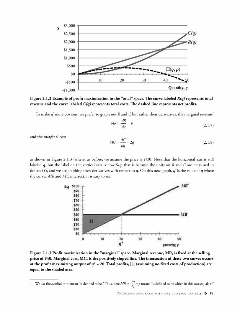
Fig ure 2.1.2 Example of profi t maximization in the “total” space. Th e curve labeled R(q) represents total revenue and the curve labeled C(q) represents total costs. Th e dashed line represents net profi ts.

To make q* more obvious, we prefer to graph not R and C but rather their derivatives, the marginal revenue*

: dRMR pdq

(2.1.7)

and the marginal cost : 2dCMC q

dq (2.1.8)

as shown in Figure 2.1.3 (where, as before, we assume the price is $40). Note that the horizontal axis is still labeled q, but the label on the vertical axis is now $/q; that is because the units on R and C are measured in dollars ($), and we are graphing their derivatives with respect to q. On this new graph, q* is the value of q where the curves MR and MC intersect; it is easy to see.

Fi gure 2.1.3 Profi t maximization in the “marginal” space. Marginal revenue, MR, is fi xed at the selling price of $40. Marginal cost, MC, is the positively sloped line. Th e intersection of these two curves occurs at the profi t maximizing output of q* = 20. Total profi ts, ∏, (assuming no fi xed costs of production) are equal to the shaded area.

* We use the symbol ú to mean “is defi ned to be.” Th us, here MR ú dR⎯dq

= p means “is defi ned to be which in this case equals p.”


We can also see the second-order condition in Figure 2.1.3. To the left of ,q the marginal benefi ts curve lies

above the marginal cost curve (meaning q

is positive), whereas to the right of ,q the marginal benefi ts

curve lies below the marginal cost curve (meaning q

is negative). Th is shows that 2

2q

is negative at ,q

the second-order condition for q to be a local maximum.

Th is graph also shows profi ts, , as the shaded area in Figure 2.1.3. Indeed, , , ,q p R q p C q

which by the Fundamental Th eorem of Calculus is the same as 0

,q

MR q MC q dq

is equal to the area of

the shaded region. To distinguish the diff erent graphs, we refer to the graph in Figure 2.1.2 as being in the total space and the graph in Figure 2.1.3 as being in the marginal space.

We can study more subtle questions. For a given price p, the fi rm will produce q p and, hence, will have profi t ,q p p , a function of just p. We call this function * ; i.e., we defi ne:

* : , .p q p p Here we have:

2 2

* .2 2 4p p pp p

We call the indirect profi t function. In math terms, ∏ (the direct profi t function) is a function of both p and q, whereas is a function of just p. In economic terms, ∏ is an accounting defi nition that tells you the profi t for every quantity q and every price p, whereas tells you the profi t earned when the fi rm produces the profi t-maximizing quantity q for any given price p.

We can also take derivatives of q* and * with respect to p:

12

dq pdp

and

2 .4 2

d p p pdp

Both of these derivatives are positive. Th is result tells us : If the selling price rises, the fi rm will produce more and earn a higher profi t. Economists refer to results given in (2.1.11) and (2.1.12) as comparative statics; testable hypotheses result when the comparative statics can be given a sign.

We can also see the signs of dqdp

and d

dp

in the marginal space. Suppose that the price increases from

0 $40p to 1 $50.p Th e marginal revenue MR will increase from $40 to $50, but the marginal cost MC does

not involve p and so will not change. In Figure 2.1.4 we redraw Figure 2.1.3, adding another marginal revenue

curve for the new price $50. Th e intersection of the new marginal revenue curve and the marginal cost curve

gives a profi t-maximizing quantity 1q p that is bigger than 0q p . (Th is increase in output is as it should be,

because calculus told us that dqdp

is positive.) Th e total profi t, seen as the area between the marginal revenue and

(2.1.9)

(2.1.10)

(2.1.11)

(2.1.12)


marginal cost curves, has also increased by the amount shown with cross-hatching, which agrees with our calcu-

lation that ddp

is positive.

Figure 2.1.4 Th e impact of an increase of the price from $40 to $50 as s hown in the marginal space. As a result of the price increase, output increases from 20 to 25 and profi ts increase by the amount shown by the cross-hatched area.

Exercises

2.1.1 A fi rm produces wine that gets better with age logarithmically. Th e fi rm, of course, has to pay for the cost of storing the wine while it ages. We model this problem as follows: let t be the length of time the fi rm allows the wine to age before bottling it and taking it to market. Assume that the cost of holding the wine is fi xed at c per unit time and that the fi rm expects to sell the wine at a price of p per bottle. Th e fi rm wants to take the wine to market at the time t that maximizes its profi ts per unit bottle of wine, where profi ts are given by:

, , ln 1 .t c p p t ct

(a) Find the fi rst-order condition. Draw a sketch in the marginal space illustrating the fi rst-order condition. Label the axes and the equilibrium output.

(b) Show that the solution, t *, of the fi rst-order condition is a global maximum for .

(c) Calculate and fi nd the sign of * ,t p cp

. Illustrate this result graphically in the marginal space.

2.1.2 In this problem a monopolist faces the demand curve: p a bq , where a and b are positive param-eters. Suppose that the monopolist faces a constant marginal cost , c,and a per unit tax, t, that fi xed costs are equal to zero.

(a) Find the profi t-maximizing levels of output q and price p . Find the maximum profi t func-tion, * t . What impact will an increase in the tax rate have on the price, output, and profi t? Illustrate these results graphically.


(b) Find the tax rate t that maximizes the total tax paid to the government. Illustrate your answer graphically in the marginal space. Include the total tax in your illustration.

2.2 PROFIT MAXIMIZATION IN GENERAL

In the previous section, we worked an example where we had an explicit formula for the cost function C q . But that’s not very realistic. So let’s forget about this explicit formula and try to do all the same things we

did before but with the intention of deriving a more general result, one that is not dependent on the particular cost function chosen. We assume that the economic problem facing the fi rm’s owner is to choose the level of output, q, that maximizes its profi t, ∏, given the price level, p:

, ,q

Max q p pq C q

where C q is the fi rm’s cost function. Following the traditional assumption of diminishi ng marginal product, we assume the cost function is such that C q and C '' q are positive for all relevant values of q.*

In these types of optimization problems, we refer to the variables that the optimizer can control as the control variables. It is traditional to list the control variables below the “Max” in order to clearly diff erentiate between these variables and the parameters of the model. In this model the only control variable is q because it is the only variable the fi rm decision-makers can use to aff ect profi ts .

Solving (2.2.1) is a straightforward optimization problem covered in beginning calculus courses. In general, a function of one variable is at a (local) maximum if (1) its fi rst derivative with respect to the control variable is equal to zero while (2) its second derivative is negative. We refer to these two conditions for maximization as the fi rst-order and second-order conditions. Th us, an output level, say q* , satisfi es the fi rst-order condition if

, 0q p p C qq

.

Let’s assume that such a q* exists. (Otherwise we are talking about an unusual or uninterest ing economic situa-tion.) Th e second-order condition is:

2

2 , 0,q p C qq

which holds because we assumed that C q is positive for all relevant q. So q* is a local maximum . Furthermore,

since 2

2 C qq

is negative for all relevant values of q, q is even a global maximum by the Global SOC

Th eorem 1.2.1.

Illustration of the solution to the profi t maximization problem

Economists traditionally illustrate the fi rst-order conditions given by (2.2.2) with the graph given in Figure 2.2.1. In this fi gure we show marginal costs, C q , as positively sloped because of the second-order conditions.

* Th e phrase “all relevant values of q” is vague on purpose. Basically, economists (unlike mathematicians) are interested only in reasonable solutions. Th us, economists do not care (or think about) what happens to the cost function either for negative levels of output or for values of output that are unreasonably large.

(2.2.1)

(2.2.2)

(2.2.3)


Th e intersection of the price line, p, with the marginal cost curve defi nes the level of output, q* , that maximizes pro fi ts.

Figure 2.2.1 Illustration of the fi rst-order conditions. Th e profi t-maximizing output, q* , is the lev el of output where the marginal cost curve, C q , intersects the marginal revenue curve, p.

Figure 2.2.1 is typical of the sorts of graphs in marginal space that we examine in this book. Th e horizontal axis is labeled with a control variable (here, q), the vertical axis is labeled with $/q (more generally, $ per units of the control variable), the graph shows marginal costs and marginal benefi ts, and the q-value of their intersec-tion is labeled with q .

A graph of the fi rst-order condition is particularly useful for illustrating the impact of a change in the level of a parameter on the equilibrium level of the control variable. Figure 2.2.2, for instance, illustrates the impact of a rise in the price for 0p to 1p on the equilibrium level of output, which rises from 0q p to 1q p . Th at

is, dq pdp

is positive. An important thing to notice here is that we view the solution to the fi rst-order condi-

tions, q* , as a function of price, p: q p . We now justify why we can d o this.

Figure 2.2.2 A rise in the price from 0p to 1p causes output to rise from 0q p to 1 .q p


2.3 EXISTENCE OF A SOLUTION TO THE PR OFIT MAXIMIZATION PROBLEM

Th ere is no reason to expect that a solution to the fi rst-order conditions necessarily exists. For instance, if the price p always falls below marginal costs, the marginal space will be as in Figure 2.3.1, and no solution to the fi rst-order conditions will exist. But for such a low price, the fi rm will produce no output, so this situation is not of much interest to economists who more often are interested in why a fi rm exists and produces some output than in when a fi rm does not exist. In this example, there is some price 0p and some quantity 0q such that the fi rst-order conditions 0 0p C q holds and the second-order condition 0 0C q holds. Indeed, if you pick any 0 0p C , then the curves 0p and C q will intersect at a point 0 0,q p . Th e second-order condition holds by (2.2.3). Th en the Implicit Function Th eorem says that the quantity q* is a function of p for prices near

0p . For more details, see section 2.7.

Figure 2.3.1 Th e fi rm will not produce anything if prices are too low.

We will typically assume that a solution to the fi rst -order and second-order conditions exists and is a func-tion of the parameters. As in the previous paragraph, we know that this assumption is a mild assertion thanks to the Implicit Function Th eorem .

Moreover, it is typical for the economist also to assume that the second-order conditions to the maximization problem are satisfi ed for all q and not just for q . In this model the assumption that the sign of the second-de-rivative of the cost function is positive for all relevant output levels guarantees that the second-order condition C q* 0 holds.

2.4 COMPARATIVE STATICS

Th e real usefulness of the fact that we can write the equilibrium level of output as a function of the parameters of the model (in our example, q is a function of p) is that we can use this result to derive comparative static results that we then can use to test the validity of the model. Formally, here is how we do it:

(1) Assume that a solution to the fi rst-order conditions exists and is given by :q q p .(2) Substitute this solution into the fi rst-order conditions (2.2.2) to get the identity:

0 for all .p C q p p (2.4.1)


(3) Diff erent iate the resulting equation (2.4.1) with respect to the parameter p:

1 0.dq p

C q pdp

(4) Solve for the derivative in the equation a nd attempt to determine the sign of the derivative as predicted by the model:

1 0.dq p

dp C q p

Th is last result is a testable implication of our model. In theory, we could examine data from the real world and see if output and prices are positively correlated. If they were negatively correlated, we would have to reject at least one of the assumptions in the model; if they are positively correlated, then we cannot reject the theory in our model.

We can derive a second kind of comparative static* result in these optimization problems. We begin by substituting the solution to our problem into the (direct) profi t function to get what is defi ned to be the indirect profi t funct ion :

: ,p q p p

or

.p pq p C q p

Diff erentiation of the indirect profi t function with respect to the price, p, yields the second comparative static :

d p dq p dq pq p p C q p

dp dp dp

d p dq pq p p C q p

dp dp

or , since the fi rst-order condition implies 0p C q p , we get:

0.d p

q pdp

Th ere is a useful thing to note in this fi nal result. Th e direct profi t function is:

, .q p pq C q

Diff erentiation of the direct profi t func tion with respect to the parameter, p, yields:

,, .p

q pq p q

p

* Mathematicians say “sensitivity analysis” rather than comparative statics, but their focus is also diff erent. We are only looking

for coarse information like the sign of dq pdp

whereas they are interested in numerical values.

(2.4.2)

(2.4.3)

(2.4.4)

(2.4.5)

(2.4.6)


If we substitute the solution of the fi rst-order condition, q p , into this last result, we get :

, .p q p p q p

Combining this with E quation (2.4.6), we see that

d p dp

p q p , p .

Equation (2.4.7) says that the derivative of the indirect profi t function with respect to price, p, is equal to the deriva-tive of the direct profi t function with respect to price with the solution to the fi rst-order conditions substituted into the equation. Equation (2.4.7) is an example of a theorem we will prove time and again in this book; it is known as the Envelope Th eorem .

Exercises

2.4.1 A fi rm in a competitive market has the following cost function:

C(q,β) = qβ,where β > 1. Assume that the fi rm sells its product at a price p.

(a) Find q* (p,β) and the indirect profi t function ∏* (p,β).

(b) Find ∂q* (p,β)⎯⎯⎯⎯∂p . Determine its sign.

(c) Find ∂q* (p,β)⎯⎯⎯⎯∂β . Determine its sign. [Hint: the sign depends on the values of p and β .]

(d) Find ∂∏* (p,β)⎯⎯⎯⎯∂p . Determine its sign.

2.4.2. Assume that a fi rm is operating in a perfectly competitive market so that the managers of the fi rm view the selling price of its product, p, as being outside of their control. Assume that the fi rm chooses the level of output that maximizes its profi ts and that the fi rm is subject to a per unit output tax, t.* Th e fi rm’s revenue function is:

R (q, p) = pq − tq.Th us, the model in this problem is:

Max ∏ (q, p, t) = pq − tq − C(q). q

* You will see per unit output taxes handled two ways in economics textbooks. In some cases the tax is treated as a part of costs, which becomes production costs, plus tax costs, In other cases they are considered as part of revenues—that is, the revenue the producer “sees” is equal to the revenue the consumer (price time quantity) pays minus the tax revenue (tax rate times quantity) paid to the government. Th ese two ways of treating taxes are equivalent in the sense that the results of the analysis are the same. For convenience, we will treat the tax revenue as part of the revenue function of a fi rm.

(2.4.7)


(a) Write the fi rst- and second-order conditions for the model. What assumptions are required on the cost function in order that the second-order condition is satisfi ed? Illustrate the fi rst-order condition with a sketch in the marginal space.

(b) Th e tax, t, enters the model as a parameter. Suppose that there is a solution ,q t p to the fi rst-order

condition and that the second-order condition holds. Determine the sign of ,q t pt

using calculus. Draw a sketch in the marginal space illustrating this result.

(c) Let ,p t be the maximum profi t as a function of p and t. Determine the sign of ,p tt

. Draw a

sketch in the marginal space illustrating this result.

2.4.3. Assume that a monopolist chooses the price, p, that maximizes her fi rm’s profi ts. Th e fi rm faces a de-mand given by D p , where 0D p . Assume that the fi rm faces constant average costs, c. Th us, the fi rm’s profi t function is ,p c pD p cD p .

(a) What is the fi rm’s fi rst-order condition?(b) What is the fi rm’s second-order condition?(c) Let p c be a solution to the fi rst-order condition and suppose that the second-order condition holds.

Find and sign dp cdc

.

(d) Defi ne the markup of price over costs to be :m p c . Find and sign dp cdc

and dm c

dc

under the

special assumption that the demand function D p is linear.

2.5 THE PROTOTYPICAL ECONOMIC PROBLEM

We can generalize what we have been doing by considering the following typical economic problem: An economic actor has a variable she can control, say x. When she chooses x, she receives some benefi ts, B(x,α), while facing some costs, C(x,α), where α is a vector of parameters. We assume that the individual chooses the level of x with the intent of maximizing the net benefi ts she receives. Th us, her economic problem is:

Max ∏ (x,α) = B(x,α) − C(x,α). (2.5.1) x

Solve for a solutionTh e fi rst-order condition for this problem is:

∏x (x,α) = B(x,α) − C(x,α) = 0. (2.5.2)

Suppose we have a solution x* to this equation. Th en the second-order condition is

∏x (x*,α) = Bx(x

*,α) − Cx(x*,α) < 0. (2.5.3)

(Note that we have mostly dropped the notation ∂ for derivatives and have switched to subscripts.)Equation (2.5.2) says that the individual will set her level of x such that the marginal benefi t she receives

equals her marginal cost . Equation (2.5.3) says that the slope of the marginal benefi t curve is less than the

Optimization in Microeconomics - University Readers · 2 Optimization in Microeconomics Tab le...

Documents

Transcript of Optimization in Microeconomics - University Readers · 2 Optimization in Microeconomics Tab le...