Optimization in Machine Learning - Institute for … · Optimization in Machine Learning ... of an...

Optimization in Machine Learning

Stephen Wright

University of Wisconsin-Madison

Singapore, 14 Dec 2012

Stephen Wright (UW-Madison) Optimization Singapore, 14 Dec 2012 1 / 48

1 Learning from Data: Applications and Models

2 First-Order Methods

3 Stochastic Gradient Methods (Parallel)

4 Identifying Subspaces from Partial Observations

5 Atomic-Norm Regularization

6 Optimization in Deep Learning


Outline

Give some examples of data analysis and learning problems and theirformulations as optimization problems.

Highlight common features in these formulations.

Survey some optimization techniques that are being applied to theseproblems. [Give a basic result or two for each.]

Highlight several applications and algorithms from recent work.

Optimization in learning and data analysis is a large and growing area —omit many topics of interest here.


** Data Analysis / Learning from Data

Typical ingredients of optimization formulations of data analysis problems:

A collection of data, from which we want to extract key informationand/or make inferences about future / missing data.

Parametrized Model of how the data relates to the meaning we aretrying to extract.

Objective that measures quality of information learned: includesmodel / data discrepancies and deviation from prior knowledge ordesirable structure. Model parameters are observed from data via theobjective.

Other typical properties of learning problems are huge underlying data set,and need for solutions with only low-medium accuracy.

In some cases, the optimization formulation is well settled. (e.g. LeastSquares, Robust Regression, Support Vector Machines, LogisticRegression, Recommender Systems.)

In other areas, formulation is a matter of ongoing debate!Stephen Wright (UW-Madison) Optimization Singapore, 14 Dec 2012 4 / 48

LASSO

Least Squares: Given a set of feature vectors ai ∈ Rn and outcomes bi ,i = 1, 2, . . . ,m, find weights x on the features that predict the outcomeaccurately: aTi x ≈ bi .

Under certain assumptions on measurement error, can find a suitable x bysolving a least squares problem

minx

1

2‖Ax − b‖2

2,

where the rows of A are aTi , i = 1, 2, . . . ,m.

An approximate sparse solution (few nonzeros in x) can be found from

LASSO: minx

1

2‖Ax − b‖2

2 such that ‖x‖1 ≤ T ,

for parameter T > 0. (Smaller T gives fewer nonzeros in x .)


LASSO and Compressed Sensing

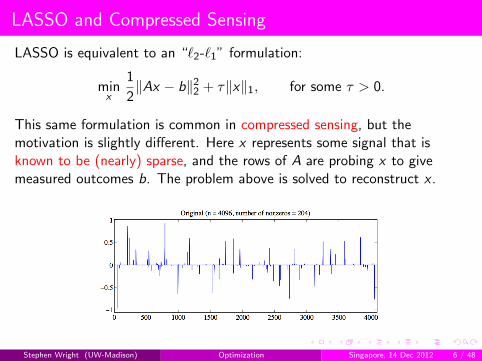
LASSO is equivalent to an “`2-`1” formulation:

minx

1

2‖Ax − b‖2

2 + τ‖x‖1, for some τ > 0.

This same formulation is common in compressed sensing, but themotivation is slightly different. Here x represents some signal that isknown to be (nearly) sparse, and the rows of A are probing x to givemeasured outcomes b. The problem above is solved to reconstruct x .


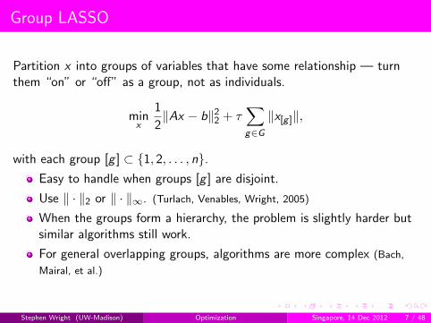
Group LASSO

Partition x into groups of variables that have some relationship — turnthem “on” or “off” as a group, not as individuals.

minx

1

2‖Ax − b‖2

2 + τ∑g∈G‖x[g ]‖,

with each group [g ] ⊂ 1, 2, . . . , n.Easy to handle when groups [g ] are disjoint.

Use ‖ · ‖2 or ‖ · ‖∞. (Turlach, Venables, Wright, 2005)

When the groups form a hierarchy, the problem is slightly harder butsimilar algorithms still work.

For general overlapping groups, algorithms are more complex (Bach,

Mairal, et al.)


Least Squares with Nonconvex Regularizers

Nonconvex element-wise penalties have become popular for variableselection in statistics.

SCAD (smoothed clipped absolute deviation) (Fan and Li, 2001)

MCP (Zhang, 2010).

Properties: Unbiased and sparse estimates, solution path continuous inregularization parameter τ .

SparseNet (Mazumder, Friedman, Hastie, 2011): coordinate descent.Stephen Wright (UW-Madison) Optimization Singapore, 14 Dec 2012 8 / 48

Linear Support Vector Classification


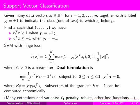
Support Vector Classification

Given many data vectors xi ∈ Rn, for i = 1, 2, . . . ,m, together with a labelyi = ±1 to indicate the class (one of two) to which xi belongs.

Find z such that (usually) we have

xTi z ≥ 1 when yi = +1;

xTi z ≤ −1 when yi = −1.

SVM with hinge loss:

f (z) = CN∑i=1

max(1− yi (zT xi ), 0) +

1

2‖z‖2,

where C > 0 is a parameter. Dual formulation is

minα

1

2αTKα− 1Tα subject to 0 ≤ α ≤ C1, yTα = 0,

where Kij = yiyjxTi xj . Subvectors of the gradient Kα− 1 can be

computed economically.

(Many extensions and variants: `1 penalty, robust, other loss functions,...)Stephen Wright (UW-Madison) Optimization Singapore, 14 Dec 2012 10 / 48

(Regularized) Logistic Regression

Seek odds of class membership rather than a bald prediction. Binary,linear case: linear function with unknown weights z ∈ Rn:

p+(x ; z) := (1 + ezT x)−1, p−(x ; z) := 1− p+(z ;w).

Seek z so that p+(xi ; z) ≈ 1 when yi = +1 and p−(xi ; z) ≈ 1 whenyi = −1. Scaled, negative log likelihood function L(z) is

L(z) = − 1

m

∑yi=−1

log p−(xi ; z) +∑yi=1

log p+(xi ; z)

Regularize: To get a sparse z (i.e. classify on the basis of a few features):

minzL(z) + λ‖z‖1.


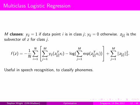
Multiclass Logistic Regression

M classes: yij = 1 if data point i is in class j ; yij = 0 otherwise. z[j] is thesubvector of z for class j .

f (z) = − 1

N

N∑i=1

M∑j=1

yij(zT[j]xi )− log(

M∑j=1

exp(zT[j]xi ))

+M∑j=1

‖z[j]‖22.

Useful in speech recognition, to classify phonemes.


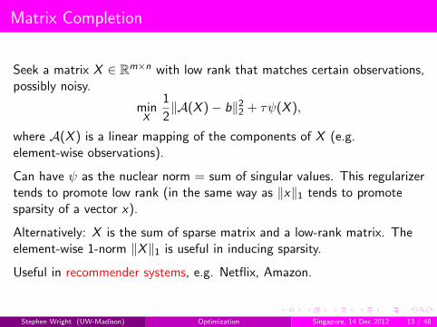
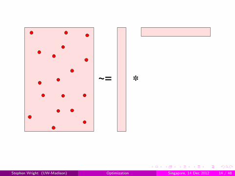
Matrix Completion

Seek a matrix X ∈ Rm×n with low rank that matches certain observations,possibly noisy.

minX

1

2‖A(X )− b‖2

2 + τψ(X ),

where A(X ) is a linear mapping of the components of X (e.g.element-wise observations).

Can have ψ as the nuclear norm = sum of singular values. This regularizertends to promote low rank (in the same way as ‖x‖1 tends to promotesparsity of a vector x).

Alternatively: X is the sum of sparse matrix and a low-rank matrix. Theelement-wise 1-norm ‖X‖1 is useful in inducing sparsity.

Useful in recommender systems, e.g. Netflix, Amazon.


*~=


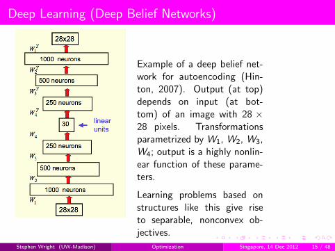
Deep Learning (Deep Belief Networks)

Example of a deep belief net-work for autoencoding (Hin-ton, 2007). Output (at top)depends on input (at bot-tom) of an image with 28 ×28 pixels. Transformationsparametrized by W1, W2, W3,W4; output is a highly nonlin-ear function of these parame-ters.

Learning problems based onstructures like this give riseto separable, nonconvex ob-jectives.


Deep Learning in Speech Processing

(Sainath et al, 2012).Break a stream of audiodata into phonemes andaim to learn how to iden-tify them from a labelledsample. May use context(phonemes before and af-ter).

Every second layer has ≈103 inputs and outputs;the parameter is the trans-formation matrix from in-put to output (≈ 106 pa-rameters).


Deep Learning

Deep learning networks typically consist of layers mapping inputs (formbelow) to outputs (to above).

Feature vectors are the inputs at the bottom layer. Classification is appliedto outputs from the top layer (e.g. SVM, multiclass logistic regression).

Individual layers are simple. Common examples:

Input vector x ∈ Rn maps to output vector y ∈ Rm as y = Wx . Themn entries of W are the parameters.

Parametrized sigmoid mapping single input to single output:yi = 1/(1 + e−βixi ).

Softmax: yi = exi/∑n

j=1 exj .

Total-variation (spatial gradient) terms to emphasize edges in imageprocessing

When composed, the result is a complicated nonconvex mapping.


Deep Learning

Neural networks were popular and well studied in the early days ofmachine learning. The equivalence between “back-propagation” andsteepest descent was recognized early and studied by several optimizationresearchers (Mangasarian, Tseng, Luo,...)

Structure of deep networks is motivated by arrangement of corticalneurons in the brain.

They lost popularity becase of the difficulty of “training”. Numerous tricksdiscovered since about 2007 have led to new success, and there has beensuccess in new big-data applications, in speech and image processing. Twonew York Times front-page stories in recent months.

Optimization techniques are front and center. More later...


Regularization Induces Structure

Formulations may include regularization functions to induce structure:

minx

f (x) + τψ(x) OR minx

f (x) s.t. φ(x) ≤ M,

where ψ induces the desired structure in x . ψ often nonsmooth.

‖x‖1 to induce sparsity in the vector x (variable selection / LASSO);

SCAD and MCP: nonconvex regularizers to induce sparsity, withoutbiasing the solution;

Group regularization / group selection;

Nuclear norm ‖X‖∗ (sum of singular values) to induce low rank inmatrix X ;

low “total-variation” in image processing;

generalizability (Vapnik: “...tradeoff between the quality of theapproximation of the given data and the complexity of theapproximating function”).


Properties of f in Data Analysis Problems

Objective f can be derived from Bayesian statistics + maximum likelihoodcriterion. Can incorporate prior knowledge.

f have distinctive properties in several applications:

Partially Separable: Typically

f (x) =1

m

m∑i=1

fi (x),

where each term fi corresponds to a single item of data, and possiblydepends on just a few components of x .

Cheap Partial Gradients: subvectors of the gradient ∇f may beavailable at proportionately lower cost than the full gradient.

These two properties are often combined.


** First-Order Methods

Fundamental first-order methods are the basis of many algorithms. Theycan typically be extended for

nonsmooth-regularized f ;

simple constraints x ∈ Ω;

availability of just a random approximation to ∇f .

Machine learning people love theorems about convergence behavior onconvex problems:

linear / geometric.

sublinear: 1/k , 1/k2, etc.

dependence of rate on dimension n and amount of data T .

Sometimes improvements in theoretical rates are reflected in practice e.g.steepest-descent vs accelerated methods.

The question: “What can we say about the nonconvex case?” is especiallyrelevant in deep learning.


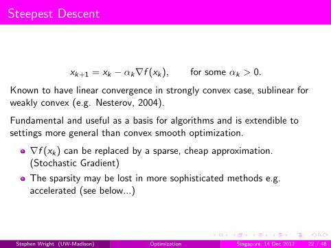
Steepest Descent

xk+1 = xk − αk∇f (xk), for some αk > 0.

Known to have linear convergence in strongly convex case, sublinear forweakly convex (e.g. Nesterov, 2004).

Fundamental and useful as a basis for algorithms and is extendible tosettings more general than convex smooth optimization.

∇f (xk) can be replaced by a sparse, cheap approximation.(Stochastic Gradient)

The sparsity may be lost in more sophisticated methods e.g.accelerated (see below...)


Momentum

Can get dramatic improvements in convergence using momentum:

xk+1 = xk − αk∇f (xk) + βk(xk − xk−1).

Search direction is a combination of previous search direction xk − xk−1

and latest gradient ∇f (xk). Methods in this class include:

Heavy ball;

Conjugate gradient;

Accelerated first-order methods are very similar. They typicallyseparate the steepest descent step from the momentum step togenerate two or three interleaved sequences.

Momentum term stores information from previous iterates and graduallyphases it out.


Momentum Methods

Denoting κ = condition number, heav-ball sets

αk ≡4

L

1

(1 + 1/√κ)2

, βk ≡(

1− 2√κ+ 1

)2

.

to get a linear convergence rate with constant approximately 1− 2/√κ.

Contrast with rate of 1− 1/κ for steepest descent. Results in a factor of√κ improvement in work to achieve a given accuracy ε.

Conjugate gradient is motivated quite differently, but has the same formand achieves a similar convergence rate. CG makes a more adaptive choiceof αk and βk .


** Stochastic Gradient Methods

Still deal with (weakly or strongly) convex f . But change the rules:

Allow f nonsmooth.Don’t calculate function values f (x).Can evaluate cheaply an unbiased estimate of a vector from thesubgradient ∂f .

A useful form of f for these methods in learning problems is

f (x) =1

m

m∑i=1

fi (x),

where each fi is convex.

Choose index ik ∈ 1, 2, . . . ,m uniformly at random at iteration k, set

xk+1 = xk − αk∇fik (xk),

for some αk > 0.

When f is strongly convex, the analysis of convergence of E (‖xk − x∗‖2) iselementary (e.g. Nemirovski et al, 2009).

Depends on careful choice of αk , naturally. Line search for αk is not reallyan option, since we can’t (or won’t) evaluate f !


SG Variants and Convergence

Stochastic gradient can be smoothed by averaging in primal or dual.

Primal Averaging: Report weighted average of all iterates:

xT :=T∑t=1

γtxt .

(For suitable choices of γt , can keep a running tally cheaply.)

Dual averaging: Define search direction

gt :=1

T

T∑j=1

∇fij (xj).

Average of all gradient estimates seen so far.

In regularized or constrained problems, dual-averaging iterates typicallyidentify the optimal manifold finitely with high probability (Lee and Wright,

2012). (Not true for standard or primal-averaged SG.)Stephen Wright (UW-Madison) Optimization Singapore, 14 Dec 2012 26 / 48

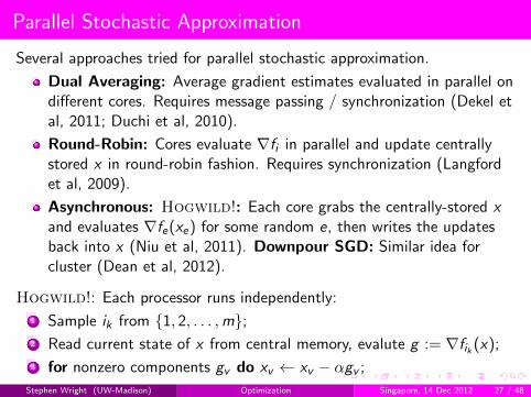
Parallel Stochastic Approximation

Several approaches tried for parallel stochastic approximation.

Dual Averaging: Average gradient estimates evaluated in parallel ondifferent cores. Requires message passing / synchronization (Dekel etal, 2011; Duchi et al, 2010).

Round-Robin: Cores evaluate ∇fi in parallel and update centrallystored x in round-robin fashion. Requires synchronization (Langfordet al, 2009).

Asynchronous: Hogwild!: Each core grabs the centrally-stored xand evaluates ∇fe(xe) for some random e, then writes the updatesback into x (Niu et al, 2011). Downpour SGD: Similar idea forcluster (Dean et al, 2012).

Hogwild!: Each processor runs independently:

1 Sample ik from 1, 2, . . . ,m;2 Read current state of x from central memory, evalute g := ∇fik (x);

3 for nonzero components gv do xv ← xv − αgv ;


Hogwild! Convergence

Updates can be old by the time they are applied, but we assume abound τ on their age.

Processors can overwrite each other’s work, but sparsity of ∇fe helps— updates to not interfere too much.

Analysis of Niu et al (2011) simplified / generalized by Richtarik (2012).

Rates depend on τ , L, µ, initial error, and other quantities that define theamount of overlap between nonzero components of ∇fi and ∇fj , for i 6= j .

For a constant-step scheme (with α chosen as a function of the quantitiesabove), essentially recover the 1/k behavior of basic SG. (Also dependslinearly on τ and the average sparsity.)


Hogwild! Performance

Hogwild! compared with averaged gradient (AIG) and round-robin (RR).Experiments run on a 12-core machine. (10 cores used for gradientevaluations, 2 cores for data shuffling.)


Hogwild! Performance


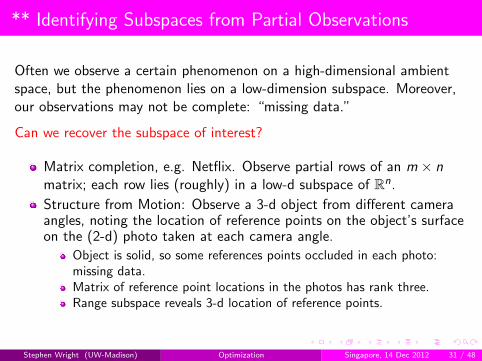
** Identifying Subspaces from Partial Observations

Often we observe a certain phenomenon on a high-dimensional ambientspace, but the phenomenon lies on a low-dimension subspace. Moreover,our observations may not be complete: “missing data.”

Can we recover the subspace of interest?

Matrix completion, e.g. Netflix. Observe partial rows of an m × nmatrix; each row lies (roughly) in a low-d subspace of Rn.

Structure from Motion: Observe a 3-d object from different cameraangles, noting the location of reference points on the object’s surfaceon the (2-d) photo taken at each camera angle.

Object is solid, so some references points occluded in each photo:missing data.Matrix of reference point locations in the photos has rank three.Range subspace reveals 3-d location of reference points.


Structure from Motion: Figures and Reconstructions

(Kennedy, Balzano, Taylor, Wright, 2012)Stephen Wright (UW-Madison) Optimization Singapore, 14 Dec 2012 32 / 48

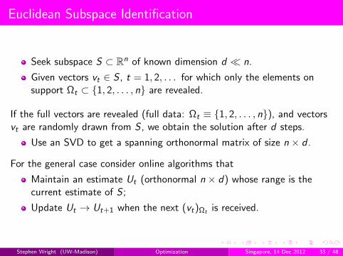
Euclidean Subspace Identification

Seek subspace S ⊂ Rn of known dimension d n.

Given vectors vt ∈ S , t = 1, 2, . . . for which only the elements onsupport Ωt ⊂ 1, 2, . . . , n are revealed.

If the full vectors are revealed (full data: Ωt ≡ 1, 2, . . . , n), and vectorsvt are randomly drawn from S , we obtain the solution after d steps.

Use an SVD to get a spanning orthonormal matrix of size n × d .

For the general case consider online algorithms that

Maintain an estimate Ut (orthonormal n × d) whose range is thecurrent estimate of S ;

Update Ut → Ut+1 when the next (vt)Ωt is received.


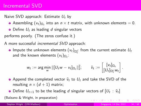
Incremental SVD

Naive SVD approach: Estimate Ut by

Assembling (vt)Ωt into an n × t matrix, with unknown elements = 0.

Define Ut as leading d singular vectors

performs poorly. (The zeros confuse it.)

A more successful incremental SVD approach:

Impute the unknown elements (vt)ΩCt

from the current estimate Ut

and the known elements (vt)Ωt :

wt := arg minw‖[Utw − vt ]Ωt‖2

2; vt :=

[[vt ]Ωt

[Ut ]Ωctwt

].

Append the completed vector vt to Ut and take the SVD of theresulting n × (d + 1) matrix;

Define Ut+1 to be the leading d singular vectors of [Ut : vt ]

(Balzano & Wright, in preparation)


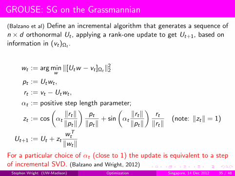
GROUSE: SG on the Grassmannian

(Balzano et al) Define an incremental algorithm that generates a sequence ofn × d orthonormal Ut , applying a rank-one update to get Ut+1, based oninformation in (vt)Ωt .

wt := arg minw‖[Utw − vt ]Ωt‖2

2

pt := Utwt ,

rt := vt − Utwt ,

αt := positive step length parameter;

zt := cos

(αt‖rt‖‖pt‖

)pt‖pt‖

+ sin

(αt‖rt‖‖pt‖

)rt‖rt‖

(note: ‖zt‖ = 1)

Ut+1 := Ut + ztwTt

‖wt‖For a particular choice of αt (close to 1) the update is equivalent to a stepof incremental SVD. (Balzano and Wright, 2012)


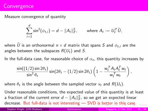
Convergence

Measure convergence of quantity

d∑i=1

sin2(φt,i ) = d − ‖At‖2F , where At := UT

t U,

where U is an orthonormal n × d matrix that spans S and φt,i are theangles between the subspaces R(Ut) and S .

In the full-data case, for reasonable choice of αt , this quantity increases by

sin((1/2) sin 2θt)

sin2 θtsin(2θt − (1/2) sin 2θt)

(1− wT

t AtATt wt

wTt wt

),

where θt is the angle between the sampled vector vt and R(Ut).

Under reasonable conditions, the expected value of this quantity is at leasta fraction of the current error d − ‖At‖2

F , so we get an expected lineardecrease. But full-data is not interesting — SVD is better in this case.


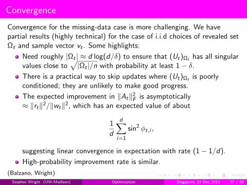
Convergence

Convergence for the missing-data case is more challenging. We havepartial results (highly technical) for the case of i.i.d choices of revealed setΩt and sample vector vt . Some highlights:

Need roughly |Ωt | ≈ d log(d/δ) to ensure that (Ut)Ωt has all singularvalues close to

√|Ωt |/n with probability at least 1− δ.

There is a practical way to skip updates where (Ut)Ωt is poorlyconditioned; they are unlikely to make good progress.

The expected improvement in ‖At‖2F is asymptotically

≈ ‖rt‖2/‖wt‖2, which has an expected value of about

1

d

d∑i=1

sin2 φt,i ,

suggesting linear convergence in expectation with rate (1− 1/d).

High-probability improvement rate is similar.

(Balzano, Wright)


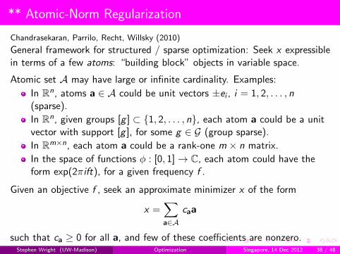
** Atomic-Norm Regularization

Chandrasekaran, Parrilo, Recht, Willsky (2010)

General framework for structured / sparse optimization: Seek x expressiblein terms of a few atoms: “building block” objects in variable space.

Atomic set A may have large or infinite cardinality. Examples:

In Rn, atoms a ∈ A could be unit vectors ±ei , i = 1, 2, . . . , n(sparse).

In Rn, given groups [g ] ⊂ 1, 2, . . . , n, each atom a could be a unitvector with support [g ], for some g ∈ G (group sparse).

In Rm×n, each atom a could be a rank-one m × n matrix.

In the space of functions φ : [0, 1]→ C, each atom could have theform exp(2πift), for a given frequency f .

Given an objective f , seek an approximate minimizer x of the form

x =∑a∈A

caa

such that ca ≥ 0 for all a, and few of these coefficients are nonzero.Stephen Wright (UW-Madison) Optimization Singapore, 14 Dec 2012 38 / 48

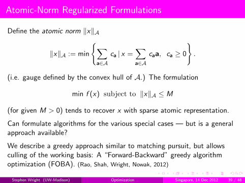
Atomic-Norm Regularized Formulations

Define the atomic norm ‖x‖A

‖x‖A := min

∑a∈A

ca | x =∑a∈A

caa, ca ≥ 0

.

(i.e. gauge defined by the convex hull of A.) The formulation

min f (x) subject to ‖x‖A ≤ M

(for given M > 0) tends to recover x with sparse atomic representation.

Can formulate algorithms for the various special cases — but is a generalapproach available?

We describe a greedy approach similar to matching pursuit, but allowsculling of the working basis: A “Forward-Backward” greedy algorithmoptimization (FOBA). (Rao, Shah, Wright, Nowak, 2012)


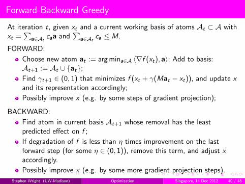
Forward-Backward Greedy

At iteration t, given xt and a current working basis of atoms At ⊂ A withxt =

∑a∈At

caa and∑

a∈Atca ≤ M.

FORWARD:

Choose new atom at := arg mina∈A 〈∇f (xt), a〉; Add to basis:At+1 := At ∪ at;Find γt+1 ∈ (0, 1) that minimizes f (xt + γ(Mat − xt)), and update xand its representation accordingly;

Possibly improve x (e.g. by some steps of gradient projection);

BACKWARD:

Find atom in current basis At+1 whose removal has the leastpredicted effect on f ;

If degradation of f is less than η times improvement on the lastforward step (for some η ∈ (0, 1)), remove this term, and adjust xaccordingly.

Possibly improve x (e.g. by some more gradient projection steps).


Implementation and Convergence

When f is linear least squares:

f (x) =1

2‖Φx − y‖2

2,

the backward step can be implemented efficiently. Enhancement stepsrequire approximate solution of

minca, a∈At+1

1

2

∥∥∥∥∥∥Φ

∑a∈At+1

caa

− y

∥∥∥∥∥∥2

2

s.t. ca ≥ 0,∑

ca ≤ M,

which is convex QP over a scaled simplex. Use projected gradient.

Convergence follows immediately from the forward-only result: (Tewari,

Ravikumar, Dhillon, 2012); see also (Zhang, 2012) and (Jaggi, 2011)

f (xT )− f (x∗) ≤ 4R/T ,

where

L := sup‖x‖A≤M

‖∇2f (x)‖, ‖A‖ := supa∈A‖a‖, R := 2LM2‖A‖2,


Convergence Proof

Denote δt := f (xt)− f (x∗). We have

f (xt + γ(Mat − xt)) ≤ f (xt) + γ〈∇f (xt),Mat − xt〉+1

2γ2L‖Mat − xt‖2

≤ f (xt) + γ〈∇f (xt),Mat − xt〉+ R

and

−δt = f (x∗)− f (xt) ≥ 〈∇f (xt), x∗ − xt〉 ≥ 〈∇f (xt),Mat − xt〉.

By substituting into previous expression we get

f (xt + γ(Mat − xt)) ≤ f (xt)− γδt + R

Subtract f (x∗) from both sides, minimize over γ ∈ [0, 1] to get

δt+1 ≤ δt − δ2t /(4R).

Result follows from an elementary recursive argument:

δt ≤4R

t⇒ δt+1 ≤ 4R

(1

t− 1

t2

)= 4R

t − 1

t2≤ 4R

t − 1

t2 − 1=

4R

t + 1.


** Deep Learning Strategies

Optimization techniques used in deep learning (in various combinations!)include:

stochastic gradient;

inexact Newton methods

with damping“Hessian-free” conjugate gradient implementation.

quass-Newton methods e.g. L-BFGS;

block coordinate descent.

Pretraining: A variant of block-coordinate descent in which all parametersexcept those for a single layer are fixed. (Single-layer problems are oftenconvex.) After one or more cycles, revert to training on the full space.

Minibatch. Random sample of data used to calculate approximategradients and Hessians. Complete pass through the data is impractical andunnecessary, as big data sets typically have a great deal of redundancy.


Stochastic Gradient in Deep Learning

Little is known about convergence properties under nonconvexity.

No evidence that the iterates terminate near a critical points / localminimum. But solution quality (as measured by classification performanceon held-out data sets) improves well as a function of training time, onmany applications.

Sometimes used as a first phase, before applying a Newton-like method.(Sainath et al, 2012)

Parallel SG used successfully on deep learning e.g. by Google group:Downpour SGD.


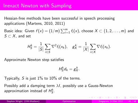
Inexact Newton with Sampling

Hessian-free methods have been successful in speech processingapplications (Martens, 2010, 2011)

Basic idea: Given f (x) = (1/m)∑m

i=1 fi (x), choose X ⊂ 1, 2, . . . ,m andS ⊂ X , and set

HkS =

1

|S |∑i∈S∇2fi (xk), gk

X =1

|X |∑i∈X∇fi (xk).

Approximate Newton step satisfies

HkSdk = gk

X .

Typically, S is just 1% to 10% of the terms.

Possibly add a damping term λI , possibly use a Gauss-Newtonapproximation instead of Hk

S .


Conjugate Gradient, Adjoint Calculations

Use conjugate gradient (CG) to find an approximate solution of theNewton-like equations. Each CG iteration requires one matrix-vectormultiplication with Hk

S , plus some vector operations (O(n) cost).

Hessian-vector product

HkSv =

1

|S |∑i∈S∇2fi (xk)v .

For sparse ∇2fi , each product ∇2fi (xk)v is cheap.

Can use an extra gradient evaluation (finite difference to approximate thisproduct). Martens (2010) suggests using adjoint techniques instead, tocompute ∇2fi (xk)v exactly. Similar to automatic differentiation — requirean “upwards sweep” followed by a “downwards sweep.”


Details

No need to iterate CG to convergence, since HkS is only an approximation

to the Hessian (and indeed the quadratic Taylor series expansion is itselfan approximation).

Typically, 2 to 50 CG iterations.

Line search along approximate Newton direction dk usually not needed;unit step suffices. The approximate Hessian sets the right scale for dk .

(Byrd et al, 2012) provide an optimization analysis of the sampled inexactNewton approach.

Sampling and coordinate descent can be combined e.g for regularizedlogistic regression Wright (2012)


Conclusions

I’ve given an incomplete survey of optimization techniques that may beuseful in analysis of large datasets, particularly for learning problems.

Some important topics omitted, e.g.

coordinate descent,

augmented Lagrangian methods / alternating direction,

quasi-Newton methods (L-BFGS),

algorithms for sparse / regularized optimization,

nonconvex regularizers,

manifold identification / variable selection.

FIN


Optimization in Machine Learning - Institute for … · Optimization in Machine Learning ... of an...

Documents

Transcript of Optimization in Machine Learning - Institute for … · Optimization in Machine Learning ... of an...