OPTIMIZATION AND EXPERIMENTAL INVESTIGATION ON EN19 USING

HEXAGONAL SHAPED ELECTRODE IN ECM

A THESIS SUBMITTED IN PARTIAL FULFILLMENT

OF THE REQUIREMENTS FOR THE DEGREE OF

Bachelor of Technology

In

Mechanical Engineering

By

ROHIT KUMAR GOUTAM

108ME039

Under the Guidance of

Dr. C. K. BISWAS

Department of Mechanical Engineering

National Institute of Technology

Rourkela

2012

i

CERTIFICATE

This is to certify that thesis entitled, “OPTIMIZATION AND EXPERIMENTAL

INVESTIGATION ON EN19 USING HEXAGONAL SHAPED ELECTRODE IN ECM”

submitted by Mr. ROHIT KUMAR GOUTAM in partial fulfillment of the requirements for the

award of Bachelor of Technology Degree in Mechanical Engineering at National Institute of

Technology, Rourkela is an authentic work carried out by him under my supervision and

guidance.

To the best of my knowledge, the matter embodied in this thesis has not been submitted to any

other university/ institute for award of any Degree or Diploma.

DATE: Dr. C. K. BISWAS

Dept. of Mechanical Engineering

National Institute of technology

Rourkela

ii

ACKNOWLEDGEMENT

Completing any task successfully precisely requires help of other fellow. I want to thank peoples

who helped me in completing my work successfully.

I want to express my gratitude and deep regards to my project supervisor, Dr. C.K. Biswas,

Associate professor, Dept. of Mechanical Engineering, NIT Rourkela for kindly providing me to

work under his supervision and guidance. I extend my deep sense of indebtedness and gratitude

to him first for his valuable guidance, constant encouragement & kind co-operation throughout

period of work which has been instrumental in the success of thesis.

I express my sincere thanks to Mr. Shailesh Kumar Dewangan, Research Scholar and Mr. Kunal

Nayak, Sr. Technical assistant, Production Engineering Laboratory, ME Dept. at NIT Rourkela

for helping me in completing my job on time.

DATE: ROHIT KUMAR GOUTAM

108ME039

iii

ABSTRACT:-

Electrochemical machining (ECM) has inaugurated itself as one of the major other possible way

to conventional methods for machining hard materials and complicated outlines not having the

residual stresses and tool wear. Electrochemical machining has vast application in automotive,

Aircrafts, petroleum, aerospace, textile, medical and electronic industries. Studies on Material

Removal Rate (MRR) are of extremely important in ECM, since it is one of the factors to be

Determined in the process decisions. So the aim of present work is to investigate the metal

removal rate, overcut diameter and surface roughness of EN19 alloy steel of diameter 13cm as

work piece by using hexagonal shaped Brass electrode and brine solution as electrolyte by using

Taguchi approach. Then optimizing to find best setting of process variables for higher MRR,

lower surface roughness and overcut. Three parameters were chosen as process variables are:

voltage, tool Feed rate and Electrolyte concentration.

Result shows that

1 Among 3 factors feed rate is effecting MRR most then comes voltage and at last electrolyte

concentration.

2 For surface roughness, feed rate effects it most then concentration and at last voltage.

3 Tool feed rate effects most to overcut at second rank is voltage and at third rank is

concentration which affects most to overcut.

4 In optimizing the quality loss function, it is found that experiment run no 5 is most optimal

i.e. voltage=10V, tool feed rate= 0.4 mm/min and electrolyte concentration =22.03g/l for

maximizing MRR and minimizing both overcut and surface roughness.

.

iv

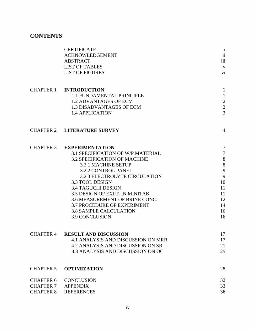
CONTENTS

CERTIFICATE i

ACKNOWLEDGEMENT ii

ABSTRACT iii

LIST OF TABLES v

LIST OF FIGURES

vi

CHAPTER 1 INTRODUCTION 1

1.1 FUNDAMENTAL PRINCIPLE 1

1.2 ADVANTAGES OF ECM 2

1.3 DISADVANTAGES OF ECM 2

1.4 APPLICATION

3

CHAPTER 2 LITERATURE SURVEY

4

CHAPTER 3 EXPERIMENTATION 7

3.1 SPECIFICATION OF W/P MATERIAL 7

3.2 SPECIFICATION OF MACHINE 8

3.2.1 MACHINE SETUP 8

3.2.2 CONTROL PANEL 9

3.2.3 ELECTROLYTE CIRCULATION 9

3.3 TOOL DESIGN 10

3.4 TAGUCHI DESIGN 11

3.5 DESIGN OF EXPT. IN MINITAB 11

3.6 MEASUREMENT OF BRINE CONC. 12

3.7 PROCEDURE OF EXPERIMENT 14

3.8 SAMPLE CALCULATION 16

3.9 CONCLUSION

16

CHAPTER 4 RESULT AND DISCUSSION 17

4.1 ANALYSIS AND DISCUSSION ON MRR 17

4.2 ANALYSIS AND DISCUSSION ON SR 21

4.3 ANALYSIS AND DISCUSSION ON OC

25

CHAPTER 5 OPTIMIZATION

28

CHAPTER 6 CONCLUSION 32

CHAPTER 7 APPENDIX 33

CHAPTER 8 REFERENCES 36

v

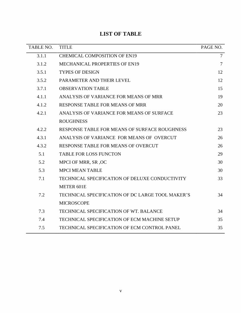
LIST OF TABLE

TABLE NO. TITLE PAGE NO.

3.1.1 CHEMICAL COMPOSITION OF EN19 7

3.1.2 MECHANICAL PROPERTIES OF EN19 7

3.5.1 TYPES OF DESIGN 12

3.5.2 PARAMETER AND THEIR LEVEL 12

3.7.1 OBSERVATION TABLE 15

4.1.1 ANALYSIS OF VARIANCE FOR MEANS OF MRR 19

4.1.2 RESPONSE TABLE FOR MEANS OF MRR 20

4.2.1 ANALYSIS OF VARIANCE FOR MEANS OF SURFACE

ROUGHNESS

23

4.2.2 RESPONSE TABLE FOR MEANS OF SURFACE ROUGHNESS 23

4.3.1 ANALYSIS OF VARIANCE FOR MEANS OF OVERCUT 26

4.3.2 RESPONSE TABLE FOR MEANS OF OVERCUT 26

5.1 TABLE FOR LOSS FUNCTON 29

5.2 MPCI OF MRR, SR ,OC 30

5.3 MPCI MEAN TABLE 30

7.1 TECHNICAL SPECIFICATION OF DELUXE CONDUCTIVITY

METER 601E

33

7.2 TECHNICAL SPECIFICATION OF DC LARGE TOOL MAKER’S

MICROSCOPE

34

7.3 TECHNICAL SPECIFICATION OF WT. BALANCE 34

7.4 TECHNICAL SPECIFICATION OF ECM MACHINE SETUP 35

7.5 TECHNICAL SPECIFICATION OF ECM CONTROL PANEL 35

vi

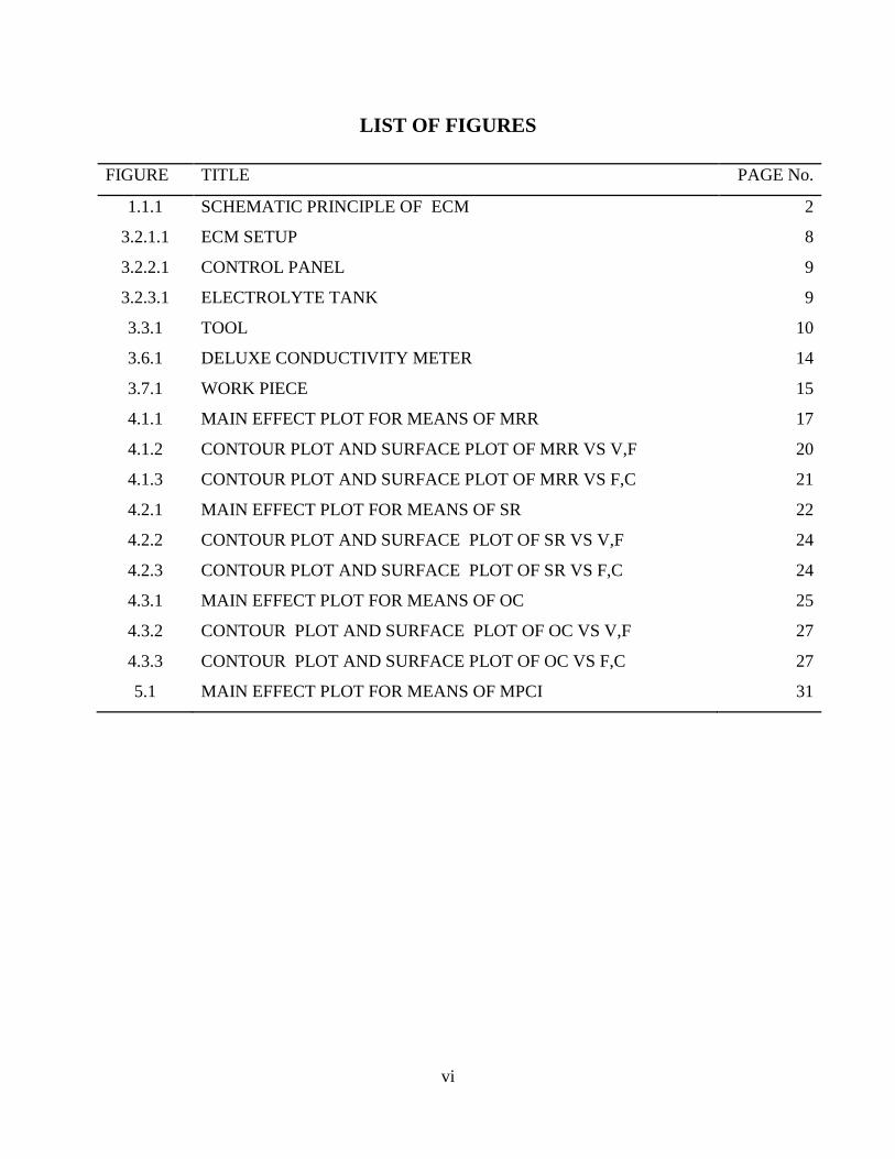
LIST OF FIGURES

FIGURE TITLE PAGE No.

1.1.1 SCHEMATIC PRINCIPLE OF ECM 2

3.2.1.1 ECM SETUP 8

3.2.2.1 CONTROL PANEL 9

3.2.3.1 ELECTROLYTE TANK 9

3.3.1 TOOL 10

3.6.1 DELUXE CONDUCTIVITY METER 14

3.7.1 WORK PIECE 15

4.1.1 MAIN EFFECT PLOT FOR MEANS OF MRR 17

4.1.2 CONTOUR PLOT AND SURFACE PLOT OF MRR VS V,F 20

4.1.3 CONTOUR PLOT AND SURFACE PLOT OF MRR VS F,C 21

4.2.1 MAIN EFFECT PLOT FOR MEANS OF SR 22

4.2.2 CONTOUR PLOT AND SURFACE PLOT OF SR VS V,F 24

4.2.3 CONTOUR PLOT AND SURFACE PLOT OF SR VS F,C 24

4.3.1 MAIN EFFECT PLOT FOR MEANS OF OC 25

4.3.2 CONTOUR PLOT AND SURFACE PLOT OF OC VS V,F 27

4.3.3 CONTOUR PLOT AND SURFACE PLOT OF OC VS F,C 27

5.1 MAIN EFFECT PLOT FOR MEANS OF MPCI 31

1

CHAPTER 1

INTRODUCTION

Electrochemical machining is a nontraditional machining process which is used to machine hard

materials which cannot be machined easily without causing any harm to tool. This can be used

for mass production and can machine external and internal of any geometry. But use of it is

limited only to electrically conductive materials.

Unlike conventional processes ECM removes metal atom by atom.it can be regarded as a

solution to a variety of metal removal problems such as cavity sinking, contouring machining

and machining helices(rifle barrels) [1].

1.1 FUNDAMENTAL PRINCIPLE:-

As ECM is controlled removal of metal by anode dissolution in an electrolyte. Removal of metal

of work piece occurs which is anode and tool is cathode. This removal of metal happens on the

principle of Faraday law of electrolysis.

Let us consider iron alloy as work piece and copper as tool and brine solution as electrolyte.

Electrolyte is mixture of NaCl and water. This breaks as

NaCl= Na++Cl

- and H2o = H

++OH

-

when potential is applied between work piece and tool negatively charged ions move towards

anode and positively charged ions move towards cathode.at cathode hydrogen ions takes electron

from cathode (tool) and becomes hydrogen gas.

2H++2e

- = H2

At anode iron ions comes out of work piece and loses two electrons and combines with chloride

ions to form iron chloride which acts as precipitate.

Fe = Fe+ +

+ 2e- and Fe

2+ + Cl

-=FeCl2

Similarly hydroxyl ions combine with sodium ions and form sodium hydroxide.

2

Na+

+ (OH) -

=NaOH

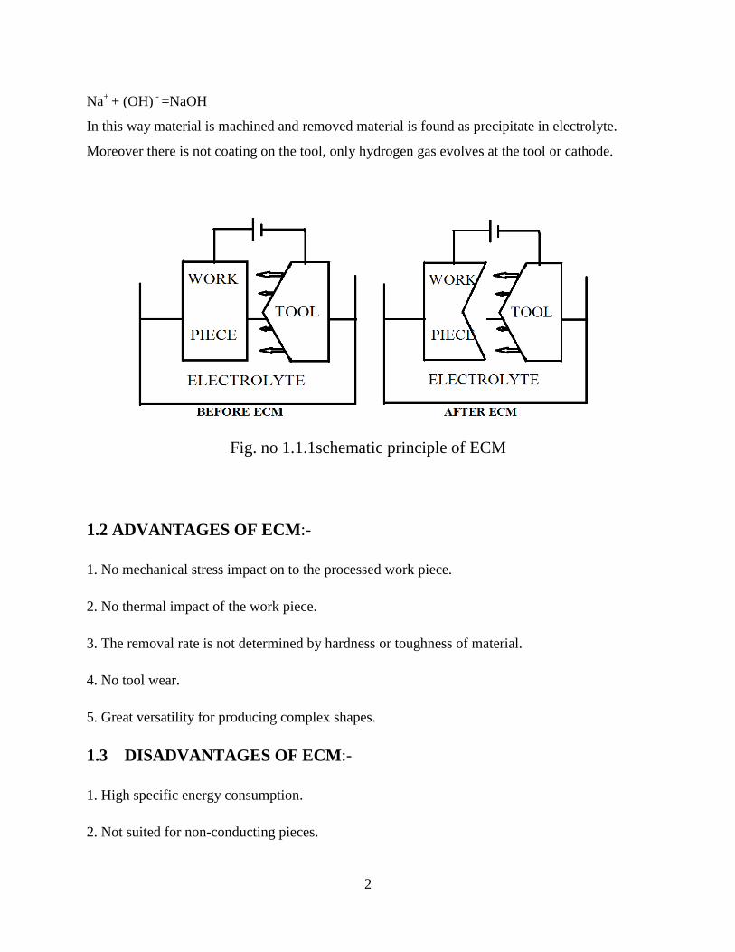
In this way material is machined and removed material is found as precipitate in electrolyte.

Moreover there is not coating on the tool, only hydrogen gas evolves at the tool or cathode.

Fig. no 1.1.1schematic principle of ECM

1.2 ADVANTAGES OF ECM:-

1. No mechanical stress impact on to the processed work piece.

2. No thermal impact of the work piece.

3. The removal rate is not determined by hardness or toughness of material.

4. No tool wear.

5. Great versatility for producing complex shapes.

1.3 DISADVANTAGES OF ECM:-

1. High specific energy consumption.

2. Not suited for non-conducting pieces.

3

3. High initial and working cost.

1.4 APPLICATION

This material can be used for making:

axial shafts

propeller shaft joint

crankshafts

high tensile bolts and studs

connecting rods

riffle barrel

gears

high tensile bolts and studs

4

CHAPTER 2

LITERATURE SURVEY

In this chapter, some research papers related to electrochemical machining are reported. They

deal with material removal rate, surface roughness, overcut, tool shape, concentration of

electrolyte, micro electrochemical machining, tool design and other responses.

T. Haisch et al. [2] they investigated anodic metal dissolution of alloyed carbon steel in

NaCl and NaNO3 as electrolyte. They applied high current densities up to 70A/cm2 and turbulent

electrolyte flow velocities in flow channel experiment. They found carbide particles on surface in

NaCl solution, which they detected using in ex situ scanning electron microscopy and energy

dispersive x ray experiment. They used auger electron microscopy with sputter depth profiling to

find film composition which resulted from NaNO3 process. They proved that increase of carbide

particles not yet separated from surrounding steel. They proposed qualitative metal dissolution

model on experimental basis for NaCl and NaNO3 as electrolyte.

B. Bhattacharyya et al. [3] in this paper tried to develop EMM experimental setup for

carrying out research for succeeding in control over EMM process parameters to meet

micromachining requirement. sets of experiments were carried out to investigate effect of

process parameters such as voltage, electrolyte concentration, and pulse on time and frequency

of power supply on MRR. According to their investigation, most effective zone of pulse on time

and electrolyte concentration is considered as 10-15ms and 15-20g/l respectively. this gives

satisfactory amount of MRR and lesser overcut .from SEM micrographs of machine jobs he

observed that lower value of electrolyte concentration with high voltage and normal pulse on

time produces more accurate shape with less overcut and normal MRR.

5

D. ChakraDhar et al. [4] they investigated the effect and parametric optimization of

process parameters for ECM of EN 31 using grey relation analysis. They considered process

parameters voltage tool feed rate and electrolyte concentration. They optimized considering

MPCI of MRR, overcut, surface roughness, cylindricity error. They observed tool feed rate is

most significant which affect ECM robustness.

C. SenthiKumar et al. [5] they investigated the influence of most important

electrochemical process parameters such as applied voltage, electrolyte concentration, tool feed

rate, electrolyte flow rate on MRR, surface roughness to fulfill effective utilization of

electrochemical machining of LM 25 Al/10%SiC composites produced through stir casting.

Contour plot generated by them to study the effect of process parameters as well their

interactions. The process parameters were optimized by RSM.

Marcio bacci da silva et al. [6] they studied the intervening variable In ECM of SAE-

XAV-F valve steel. A prototype developed by federal university of Uberlandia was used by them

for their study. They studied MRR, surface roughness and overcut. Four parameters were

changed in experiment which are feed rate, electrolyte flow rate, electrolyte, voltage .they

conducted forty experiments. They used two electrolytes NaCl and NaNO3.their result shows that

feed rate effects most to MRR. With electrolyte NaNO3 they got best result for surface

roughness and overcut.

D. Zhu et al. [7] they presented a method for studying machining accuracy in ECM using

dual pole tool with a metallic bush outside the insulated coating of cathode tool. The bush was

connected with anode so the electric field at side gap area was weakened. Simulation and

modeling presented by them shows dual pole tool decreases current density at side gap area of

the machined hole and hence reduces stray material removal. They experimentally observed that

machining accuracy and process stability significantly improved by his method.

6

H. Hochang et al. [8] in this paper, they analyzed a process to erode a hole of hundreds of

micrometers on metal surface. They presented a computational model to show machined profile

as time passes. Their analysis was based on finite width tool and fundamental law of electrolysis

.they also discussed influence of experimental variables as time of electrolysis, voltage, molar

concentration of electrolyte and electrode gap upon MRR and machined hole. Result showed that

MRR increases with increasing voltage, molar conc. Of electrolyte, time of electrolysis and

decreased initial gap. Time of electrolysis is most significant factor for hole of diameter.

AIM OF PRESENT WORK:

Aim of the present work is to find the responses, their interaction with input variables, and to

find combination of input variables to find optimum value of the response variables using

hexagonal shaped electrode on EN19 special steel as work piece in brine solution using Taguchi

approach. The input variables selected are voltage; tool feed rate and electrolyte concentration.

To find optimum value of factors we use quality loss function for higher the better (MRR) small

the better (surface roughness and overcut).

7

CHAPTER 3

EXPERIMENTATION

In this chapter, experimentation is discussed which consists about work piece specification,

Machine specification, tool design, concentration measurement, formation of the L-9 orthogonal

array based on Taguchi design and response calculations Orthogonal array decreases the total

number of experiments to be conducted. Total nine experimental runs have been conducted and

MRR, overcut diameter and surface roughness are calculated. Multi response optimization of

quality loss function is used to find best parameter setting as single response optimization cannot

be used in Taguchi design.

3.1 SPECIFICATION OF WORKPIECE MATERIAL:

The material that was selected for experiment was EN19 alloy steel .the description of the

Material EN19 alloy steel is given in table no. 4.1 and chemical composition in table 4.2and

mechanical and thermal properties are given in table no. 4.3 .the dimension of work piece is 50

mm diameter and 10 mm thickness. The work piece material is circular in shape. 2 pieces

ofEN19 alloy steel were taken to conduct 9 experiment runs .3 experiments were conducted on

each side of the work piece.

Table no. 3.1.1: chemical composition

Element C Si Mn Cr Mo S P

Weight% 0.36-0.44 0.1-0.35 0.70-1 0.9-1.20 0.25-0.35 0.035 0.040Max

Table no. 3.1.2: mechanical and thermal properties of EN19

Parameters values

density 7.700g/cm3

8

3.2 SPECIFICATION OF MACHINE:

All experiments were conducted on Electrochemical Machining set up from Metatech Industry,

Pune which have input Supply of 415 V 10%, 3 phases AC, 50 HZ and Output supply is

0-300A DC at any voltage from 0-25V. The cable insulation resistance is not less than 10 Mega

ohms with 500V DC. This machine consists of three major sub systems which are being

discussed in this Chapter.

1. Machining setup

2. Control Panel

3. Electrolyte Circulation

3.2.1 Machining setup

This electro-mechanical gathering is a strong build structure, associated with accurately

Machined components, servo motorized vertical up/down movement of tool, an electrolyte

providing arrangement, machining chamber with transparent window, job holding Arrangement,

job table lifting mechanism and strong build stand. All the exposed components are properly

insulated so to be free from corrosion. ECM setup is shown in figure 3.2.1.1

Fig no. 3.2.1.1 ECM Setup

9

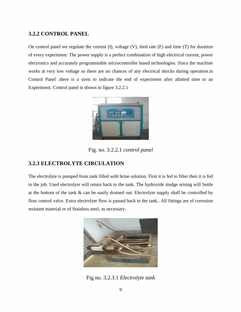
3.2.2 CONTROL PANEL

On control panel we regulate the current (I), voltage (V), feed rate (F) and time (T) for duration

of every experiment. The power supply is a perfect combination of high electrical current, power

electronics and accurately programmable microcontroller based technologies. Since the machine

works at very low voltage so there are no chances of any electrical shocks during operation.in

Control Panel .there is a siren to indicate the end of experiment after allotted time to an

Experiment. Control panel is shown in figure 3.2.2.1

Fig. no. 3.2.2.1 control panel

3.2.3 ELECTROLYTE CIRCULATION

The electrolyte is pumped from tank filled with brine solution. First it is fed to filter then it is fed

to the job. Used electrolyte will return back to the tank. The hydroxide sludge arising will Settle

at the bottom of the tank & can be easily drained out. Electrolyte supply shall be controlled by

flow control valve. Extra electrolyte flow is passed back to the tank.. All fittings are of corrosion

resistant material or of Stainless steel, as necessary.

Fig no. 3.2.3.1 Electrolyte tank

10

3.3. TOOL DESIGN

A tool is required for desired way of removing material from the work piece. Different tool

shapes are required for different use giving different shapes to the work piece for same

conditions.so a tool was made as follows:

Tool for electrochemical machining was made of brass .A solid cylindrical rod of brass of 15mm

Diameter was taken and a piece of 65mm was cut .two faces were smoothen by facing the two

Faces in lathe and maintained length 60 mm. diameter was reduced to 12mm diameter by turning

In lathe and M12 external thread was made on one end of rod using thread die as tool holder has

M12 internal thread. A through hole was made of diameter 5mm at the Centre using 5mm drill

Bit from a hexagonal shaped rod a piece of 6mm thick piece was cut. A 4mm hole was made at

Centre using 4mm drill bit .both these parts were brazed to make tool.

All dimensions are in mm

Fig. no. 3.3.1 Tool

11

3.4 TAGUCHI DESIGN:

As we know Dr. Genichi Taguchi is considered as the foremost presenter of robust parameter

Design called as Taguchi design which is a engineering method for increasing value of output or

process design that concentrates on minimizing variation and/or sensitivity to noise. When used

in precise way, Taguchi designs give a persuasive and effective method for designing products

that can operate influentially and optimally over different conditions. There are several

approaches to Experimental designs proposed by Taguchi that are sometimes called "Taguchi

Methods." two, three, four, five, and mixed-level designs are used by these methods Proposed

by Taguchi. Experimental design by Taguchi is referred as "off-line quality control" because it is

a method of being confident of getting good performance in the design stage of products or

processes.

3.5 DESIGN OF EXPERIMENT IN MINITAB

Taguchi method uses orthogonal array for arranging suitable combination of input signals in a

Table to give useful value of output responses. Orthogonal arrays are generalized Graeco Latin

squares. In a static response experiment MINITAB software provides both static and dynamic

response experiment; the quality characteristic of interest has a fixed level. The quality

Characteristic operates over a certain range of values in dynamic response experiment and aim of

This experiment is to make better the relation between input signal and output response. This

design experiment is used to find best combination of input signals or variables setting that can

achieve robustness against noise factors. MINITAB software calculates response tables and

generates main effects and interaction plot for:--

Signal to noise ratios versus input variables or control factors.

Mean versus input variables or control factors.

Standard deviation versus input variables or control factors.

Natural logarithm of standard deviation versus control factors.

12

Table no.3.5.1: types of design

2-level design 2 to 31 factors

3 level design 2 to 13 factors

4 level design 2 to 5 factors

5 level design 2 to 6 factors

mixed level design 2 to 26 factors

For my experiment I have selected 3 level design .voltage, tool feed rate, and concentration are

taken as control factors. Level of each factor is taken as 3 .so I had choice of L9 and L27

Orthogonal array. I chose L9 OA’ for my experiment.

Table no.3.5.2: parameters and their level

Parameters symbols unit Level 1 Level 2 Level3

voltage V V 7 10 13

Tool feed rate F mm/min 0.2 0.4 0.6

concentration C g/l 22.03 30.06 35

3.6. MEASUREMENT OF BRINE SOLUTION CONCENTRATION

As brine solution is a solution of sodium chloride and water.so certain quantity of sodium

Chloride is mixed in some liter of water. To measure concentration of a brine solution we can

Measure conductivity of same solution and then can convert conductivity into concentration.

Conductivity of a solution can be measured by instrument called “deluxe conductivity meter

Model no.601 E”.

13

MEASUREMENT OF CONDUCTIVITY OF BRINE SOLUTION

Functional testing:-

Connected the instrument to the AC supply and allowed it to warm up for few minutes.

Put the function switch CHECK position.

We need to see display reading if it reads 1.000 then it is all right if not then adjust it to

1.000 with the help of CAL control provided at back panel.

So the instrument was ready to use.

Operation:-

Connecting the conductivity cell:-

Wash the conductivity cell thoroughly with distilled water (before use, the cell kept in

Distilled water for at least twenty four hours).

Fit the electrode leads to input sockets provided at rear of the instrument.

Measurement procedure:-

Rinsed the conductivity cell with brine solution as conductivity of brine solution was

going to measure.

Dipped the conductivity cell in brine solution.

Set function switch to check position.

Display must read 1.000 as it was not showing 1.000 so I adjusted it with CAL control

provided at back panel.

Put the function switch to cell const. position and set the cell constant control to cell

constant value of the conducting cell which is 1.

Moved the function switch to conductivity Position and ranged the switch to appropriate

range.

Connected the conductivity cell at rear of instrument.

Set the temperature control to temperature of the solution which is set to 25˚c.

Brought the range switch at position where maximum resolution is obtained.

14

Read the display .this showed exact conductance of the brine solution at 25˚c. Unit of

conductivity was mili Siemen/cm.

Same procedure was repeated for more two times for calculating conductivity of brine

solution

.

Fig. no. 3.6.1 deluxe conductivity meter

CONVERSION OF CONDUCTIVITY TO CONCENTRATION:-

Raise the conductivity value by 1.0878

Multiply by 0.4665. This will give concentration in g/l.

3.7 PROCEDURE OF THE EXPERIMENT

Before starting, the experiment measured initial weight of the work piece so we can

Measure MRR.

Set the work piece in chamber in horizontal position and fixed in tool in tool holder in

Vertical Position.

The distance between work piece and tool tip is taken approximately 1.5mm.

After setting control parameters and duration of experiment to 5 minutes machining

started.

After 5 minutes experiment was over. Stopped the machine, taken out work piece,

cleaned properly and measured the final weight.

15

Measured the surface roughness using Talysurf and overcut using DC large tool maker’s

microscope.

Expt. Run no. 1, 5, 9 Expt run no. 2, 6, 7 Expt run no. 3,4,8

Fig no.3.7.1 work piece

Table no 3.7.1: observation

Run Voltage

(v)

TFR

(mm/

min)

Conc.

(g/l)

Initial

weight

(g)

Final

weight

(g)

Change

in weight

(g)

MRR

(mm3/min)

Avg.

surface

roughness

m)

Overcut

diameter

(mm)

1 7 0.2 22.03 177.382 177.266 0.116 3.013 6.80 0.4230

2 7 0.4 30.06 156.898 156.650 0.248 6.442 7.07 0.5055

3 7 0.6 35 157.780 157.399 0.381 9.896 4.13 0.5625

4 10 0.2 35 157.399 157.218 0.181 4.702 5.13 0.5345

5 10 0.4 22.03 177.266 176.966 0.30 7.792 8.93 0.5398

6 10 0.6 30.06 156.418 156.008 0.410 10.649 4.93 0.6150

7 13 0.2 30.06 156.650 156.418 0.232 6.026 3.2 0.5325

8 13 0.4 35 157.218 156.812 0.406 10.545 7.73 0.6195

9 13 0.6 22.03 176.96 176.479 0.487 12.649 5.80 0.6760

16

3.8 SAMPLE CALCULATION

MRR can be calculated as:-

MRR=

Overcut- diameter can be measured as:-

Overcut =

Di is internal diameter at the top of work piece.

Do is external tool diameter.

3.9 CONCLUSION

Experiments were conducted using designed hexagonal shaped brass electrode and machining

setup in Taguchi method .control factors voltage, tool feed rate and concentration were varied to

get 9 experiments.at the end MRR, diameter -overcut and surface roughness measurements were

done.

17

CHAPTER 4

RESULT AND DISCUSSION

In this chapter the analysis and discussion on responses which are MRR, surface roughness and

diameter-overcut are discussed.

4.1 RESULT AND DISCUSSION ON MRR

The machinability of a material in ECM depends on many factors as voltage ,tool feed rate

,concentration, tool diameter, tool design, electrolyte flow rate and many more.in my case of

study voltage, tool feed rate and concentration are input factors and others are kept constant.

In this two tables and six graphs are discussed.

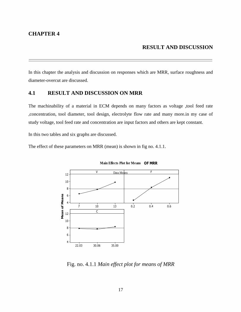
The effect of these parameters on MRR (mean) is shown in fig no. 4.1.1.

Me

an

of

Me

an

s

13107

12

10

8

6

40.60.40.2

35.0030.0622.03

12

10

8

6

4

V F

C

Main Effects Plot for Means

Data Means

OF MRR

Fig. no. 4.1.1 Main effect plot for means of MRR

18

There is large increase in MRR when feed rate increases from 0.2mm/min to 0.4mm/min than

increase in MRR when voltage increases from 7V to 10V.MRR is also more when tool feed rate

changes from 0.4mm/min to 0.6mm/min than voltage when it changes from 10V to 13V.In case

of electrolyte concentration MRR decreases slightly first till concentration is 30.06 and then

increases slightly till concentration reaches 35.

In table no. 4.1.1 column 1 represents source of variation are voltage, tool feed rate and

concentration. Column2 represents degree of freedom (DF) of each control factor which is two.

Column 3 represent sum of squares (seq. SS).column 4 represents adjusted sum of square.

Column5 represents adjusted mean of square.column6 represents F distribution and column 7

represent probability.

Significant factors are voltage and tool feed rate as their p value is less than 0.05 whereas

insignificant factor is concentration of brine solution.

Sum of square (seq. SS) is used to find amount of variation that can be explained by each factor.

Degree of freedom (DF) indicates the number of independent pieces of information involving the

response data needed to calculate the sum of squares. Degree of freedom of each component is

(n-1) where n is the number of observation.

In an ANOVA the term mean square refer to an estimate of population variance based on the

variability among a given set of measures. The calculation for mean square for model term is

MSTerm =

F-value

F-value is the measurement of the distances between individual distributions.as F value goes up

the p value goes down .F is a test to determine whether the interaction and main effects are

significant.

F =

19

P value

P value is the probability of obtaining a test statistic that is at least as extreme as actual

calculated value, if null hypothesis is true. A commonly used cut-off value for p value is 0.05.for

example if calculated p value of a test statistic is less than 0.05 we reject the null hypothesis.

Table no.4.1.1: analysis of variance for means of MRR

source DF Seq. SS Adj. SS Adj. MS F P

V 2 16.5229 16.5229 8.2615 353.49 0.003

F 2 63.4521 63.4521 31.7260 1357.47 0.001

C 2 0.7857 0.7857 0.3928 16.81 0.056

Residual error 2 0.0467 0.0467 0.0234

Total 8

S =0.1529 R-Sq. =99.9% R-Sq.(adj.) =99.8%

R-Sq. depicts the amount of variation seen in MRR and is explained by input factors. R-Sq.

=99.9% says that model is able to predict response with high accuracy. Standard deviation of

error is S=0.1529. R-Sq.(adj.) is modified R-sq. that has been adjusted for a no. of terms in

model. If unwanted terms are present in the model R-Sq. may be high but R-Sq. (adj.) may be

small. If P value is less than or equal to 0.05 then effect is considered significant otherwise not.

In table 4.1.2, the main effect of voltage, tool feed rate and electrolyte concentration on MRR

are 3.290V,6.484mm/min and 0.675g/l.in order of importance tool feed rate is more significant

and then voltage and at last brine solution concentration.

20

Table no.4.1.2: response table for means of square

level V F C

1 6.450 4.580 7.818

2 7.714 8.260 7.706

3 9.740 11.065 8.381

delta 3.290 6.484 0.675

rank 2 1 3

The calculation of MRR is done by taking the difference between model values of MRR with

observed value of MRR.

Fig no. 4.1.2 Contour plot and surface plot for MRR vs. V, F

In fig. no. 4.1.2 Contour plot of MRR versus V, F shows that with increase in voltage and tool

feed rate simultaneously MRR also increases. MRR is maximum when voltage and tool feed rate

F

V

0.60.50.40.30.2

13

12

11

10

9

8

7

MRR

6 – 8

8 – 10

10 – 12

> 12

< 4

4 – 6

Contour Plot of MRR vs V, F

21

are at maximum level.at constant voltage range of tool feed rate is increasing to give same MRR

in that range. In surface plot I see that at feed rate 0.6mm/min MRR is increasing rapidly with

increase in voltage. MRR is increasing linearly with tool feed rate at constant voltage.

C

F

343230282624

0.6

0.5

0.4

0.3

0.2

MRR

6 - 8

8 - 10

10 - 12

> 12

< 4

4 - 6

Contour Plot of MRR vs F, C

Fig no. 4.1.3 contour plot and surface plot of MRR vs. F, C

In contour plot of MRR vs. F, C MRR is increasing with increase in concentration and feed

rate.at constant feed rate MRR is nearly same for wide range of concentration. 4-6mm3/min

MRR covers more area than for other range of MRR.in surface plot at constant concentration

MRR is approx. in linear relation with tool feed rate

4.2 RESULTS AND DISCUSSION ON SURFACE ROUGHNESS

The effect of control factors voltage, tool feed rate and concentration on surface roughness are

shown in figure number 4.2.1

Surface roughness of EN19 increases slightly with increase in voltage value from 7V to 10V and

then decreases with increase in value of voltage value from 10V to13V.

22

Surface roughness of EN19 increases with increase in feed rate from 0.2mm/min to 0.4mm/min

and then decreases with increase in value of feed rate from 0.4-0.6mm/min.

In case of concentration surface roughness decreases with increase in value of concentration

from 22.03-30.06g/l and then increases with increase in concentration from 30.06-35g/l.so most

effective factor looks to be tool feed rate and then concentration.

Me

an

of

Me

an

s

13107

8

7

6

5

0.60.40.2

35.0030.0622.03

8

7

6

5

V F

C

Main Effects Plot for Means of SR

Data Means

Fig no. 4.2.1 main effect plot for means of SR

23

Table no..4.2.1: analysis of variance for means of surface roughness

source DF Seq.-ss. Adj. SS Adj. MS F P

V 2 0.8556 0.8556 0.4278 0.50 0.667

F 2 16.9678 16.9678 8.4839 9.92 0.092

C 2 7.0983 7.0983 3.5491 4.15 0.194

Residual error 2 1.7110 1.7110 0.8555

total 8 26.6327

S = 0.9249 R-Sq. = 93.6% R-Sq.(adj.) =74.3%

No factor is found to be significant as p value of all factors is greater than 0.05, to be significant

value should be less than or equal to 0.05

Standard deviation of error is 0.9249.amount of variation is 93.6% and adjusted amount of

variation is 74.3%.

Table no. 4.2.2: response table for means of surface roughness

Level V F C

1 6.000 5.043 7.177

2 6.330 7.910 5.067

3 5.577 4.953 5.663

delta 0.753 2.957 2.110

rank 3 1 2

In table no. 4.2.2 the main effect of input variables voltage, feed rate and concentration on

Surface roughness are 0.753V,2.957mm/min and 2.110g/l.

Tool feed rate is more significant and voltage is least significant. Concentration is ranked 2 in

order of significance.

24

F

V

0.60.50.40.30.2

13

12

11

10

9

8

7

SR

5 – 6

6 – 7

7 – 8

> 8

< 4

4 – 5

Contour Plot of SR vs V, F

Fig. no.. 4.2.2 Contour plot and surface plot of SR vs. V, F

In fig no. 4.2.2 contour plot shows that surface roughness >8 at Centre which looks like

elliptical region and decreases in radial direction. Minimum surface roughness <4 is obtained

when voltage is high and feed rate is low.

C

F

343230282624

0.6

0.5

0.4

0.3

0.2

SR

5 – 6

6 – 7

7 – 8

> 8

< 4

4 – 5

Contour Plot of SR vs F, C

0.6

4

0.4

SR

F

6

8

2530 0.2

C 35

Surface Plot of SR vs F, C

Fig no. 4.2.3 contour plot and surface plot of SR vs. F, C

25

Surface roughness value is minimum feed rate is low and concentration value is average. Surface

roughness value is maximum when concentration is low and feed rate is average. The region of

high surface is like parabolic area at corner of figure.

4.3 RESULT AND DISCUSSION ON DIAMETER OVERCUT

The influence of input factors on overcut-diameter is shown in diagram no. 4.3.1

Me

an

of

Me

an

s

13107

0.60

0.55

0.50

0.60.40.2

35.0030.0622.03

0.60

0.55

0.50

V F

C

Main Effects Plot for Means of overcut

Data Means

Fig. no. 4.3.1 main effect plot means of overcut

Overcut diameter increases linearly with tool feed rate .overcut diameter also increases with

increase in voltage but in piece wise linear fashion.it also increases with increase in

concentration but in piece wise linear fashion.

26

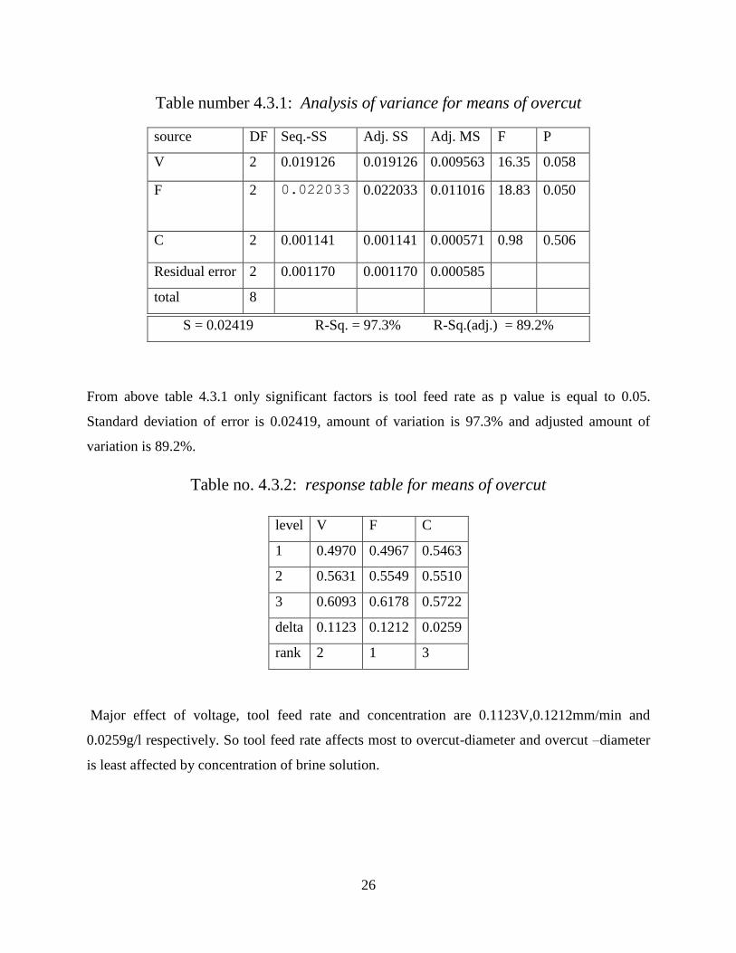
Table number 4.3.1: Analysis of variance for means of overcut

source DF Seq.-SS Adj. SS Adj. MS F P

V 2 0.019126 0.019126 0.009563 16.35 0.058

F 2 0.022033

0.022033 0.011016 18.83 0.050

C 2 0.001141 0.001141 0.000571 0.98 0.506

Residual error 2 0.001170 0.001170 0.000585

total 8

From above table 4.3.1 only significant factors is tool feed rate as p value is equal to 0.05.

Standard deviation of error is 0.02419, amount of variation is 97.3% and adjusted amount of

variation is 89.2%.

Table no. 4.3.2: response table for means of overcut

level V F C

1 0.4970 0.4967 0.5463

2 0.5631 0.5549 0.5510

3 0.6093 0.6178 0.5722

delta 0.1123 0.1212 0.0259

rank 2 1 3

Major effect of voltage, tool feed rate and concentration are 0.1123V,0.1212mm/min and

0.0259g/l respectively. So tool feed rate affects most to overcut-diameter and overcut –diameter

is least affected by concentration of brine solution.

S = 0.02419 R-Sq. = 97.3% R-Sq.(adj.) = 89.2%

27

F

V

0.60.50.40.30.2

13

12

11

10

9

8

7

OC

0.50 – 0.55

0.55 – 0.60

0.60 – 0.65

> 0.65

< 0.45

0.45 – 0.50

Contour Plot of OC vs V, F

12

0.4 10

OC

0.5

V

0.6

0.2

0.7

80.4

0.6F

Surface Plot of OC vs V, F

Fig. no. 4.3.2 contour plot and surface plot of OC vs. V, F

In figure different regions of overcut are shown. Overcut increases with increase in feed rate and

voltage, overcut is maximum in region where voltage and feed rate is max simultaneously.

C

F

343230282624

0.6

0.5

0.4

0.3

0.2

OC

0.50 – 0.55

0.55 – 0.60

0.60 – 0.65

> 0.65

< 0.45

0.45 – 0.50

Contour Plot of OC vs F, C

0.6

0.4 0.4

OC

0.5

F

0.6

0.7

2530 0.2

C 35

Surface Plot of OC vs F, C

Fig. no. 4.3.3 contour plot and surface plot of overcut vs. F, C

Overcut is max When tool feed rate is max and concentration is minimum.in surface plot when

concentration is min. then feed rate and overcut varies linearly.

28

CHAPTER 5

OPTIMIZATION

OPTIMIZATION USING QUALITY LOSS FUNCTION:-

To calculate the difference between wished value and experimental value quality loss function is

used.

Responses can come under three categories

1. Large is better

2. Normal is better

3. Small is better

In multi performance characteristic each characteristics may be in different category.so in

optimization they have to be deal in different way.

MRR comes in larger the better category and surface roughness and overcut in small is better

category.

Loss function for MRR=Lij=1/(Yij)2 Loss function for surface roughness and

overcut = Lij=(Yij)2

Yij is performance value for ith quality characteristic at jth trial

29

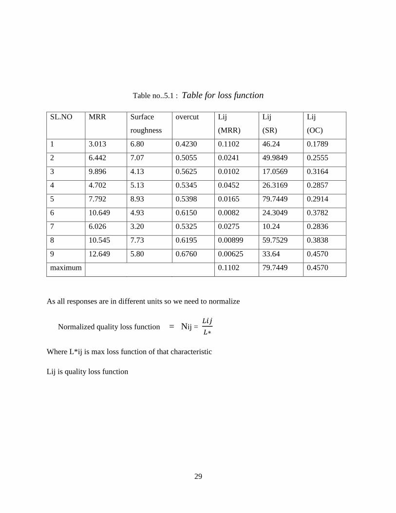
Table no..5.1 : Table for loss function

SL.NO MRR Surface

roughness

overcut Lij

(MRR)

Lij

(SR)

Lij

(OC)

1 3.013 6.80 0.4230 0.1102 46.24 0.1789

2 6.442 7.07 0.5055 0.0241 49.9849 0.2555

3 9.896 4.13 0.5625 0.0102 17.0569 0.3164

4 4.702 5.13 0.5345 0.0452 26.3169 0.2857

5 7.792 8.93 0.5398 0.0165 79.7449 0.2914

6 10.649 4.93 0.6150 0.0082 24.3049 0.3782

7 6.026 3.20 0.5325 0.0275 10.24 0.2836

8 10.545 7.73 0.6195 0.00899 59.7529 0.3838

9 12.649 5.80 0.6760 0.00625 33.64 0.4570

maximum 0.1102 79.7449 0.4570

As all responses are in different units so we need to normalize

Normalized quality loss function = Nij =

Where L*ij is max loss function of that characteristic

Lij is quality loss function

30

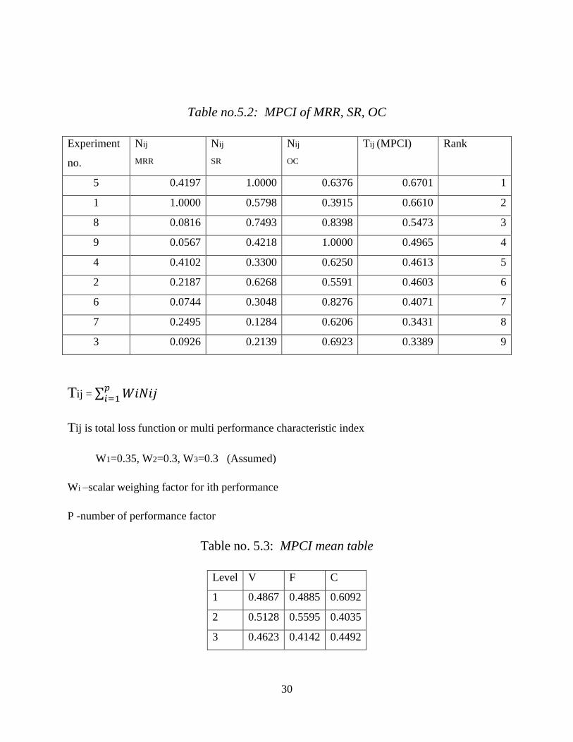
Table no.5.2: MPCI of MRR, SR, OC

Experiment

no.

Nij

MRR

Nij

SR

Nij

OC

Tij (MPCI) Rank

5 0.4197 1.0000 0.6376 0.6701 1

1 1.0000 0.5798 0.3915 0.6610 2

8 0.0816 0.7493 0.8398 0.5473 3

9 0.0567 0.4218 1.0000 0.4965 4

4 0.4102 0.3300 0.6250 0.4613 5

2 0.2187 0.6268 0.5591 0.4603 6

6 0.0744 0.3048 0.8276 0.4071 7

7 0.2495 0.1284 0.6206 0.3431 8

3 0.0926 0.2139 0.6923 0.3389 9

Tij = ∑

Tij is total loss function or multi performance characteristic index

W1=0.35, W2=0.3, W3=0.3 (Assumed)

Wi –scalar weighing factor for ith performance

P -number of performance factor

Table no. 5.3: MPCI mean table

Level V F C

1 0.4867 0.4885 0.6092

2 0.5128 0.5595 0.4035

3 0.4623 0.4142 0.4492

31

Fig. no.5.1 Main effect plot for means of MPCI

Max value of MPCI is at level 2 for voltage, at level 2 for tool feed rate and at level 1 for brine

solution concentration. So, optimum combination of responses should be 10V, 0.4mm/min and

22.03g/l.

32

CHAPTER 6

CONCLUSION

In this study of ECM process on EN19 alloy steel by hexagonal shaped electrode I considered 9

experiments by Taguchi design. .in this three factors were considered that are voltage, tool feed

rate and electrolyte conctration. These 9 experiments were conducted to obtain high MRR, low

overcut and low surface roughness. optimization by quality loss function was used to obtain

suitable combination of factors to get large MRR, small overcut and small surface roughness. I

arrived at following conclusion:-

1. Among 3 factors feed rate is effecting MRR most then comes voltage and at last electrolyte

concentration.

2. For surface roughness, feed rate effects it most then concentration and at last voltage.

3. Tool feed rate effects most to overcut at second rank is voltage and at third rank is

concentration which affects most to overcut.

4. In optimizing the quality loss function, it is found that experiment run no 5 is most optimal

i.e. voltage=10V, tool feed rate= 0.4 mm/min and electrolyte concentration =22.03g/l for

maximizing MRR and minimizing both overcut and surface roughness.

33

CHAPTER 7

APPENDIX

7.1. Technical specification of deluxe conductivity meter 601E model

Range 200 S/cm to 1000mS/cm in 5 ranges

Accuracy 1% F.S. 1 digit

Resolution 1.0 S/cm

Measuring Frequency 1000 HZ

Temperature Compensation Manual 0-50

Cell Constant 0.4 TO 1.5 adjustable

Display 3 ½ digital bright red LED display

Power Supply 230 10%, 50HZ AC

Dimensions 76 275 175 mm(approx)

Weight 2 kg (approx)

34

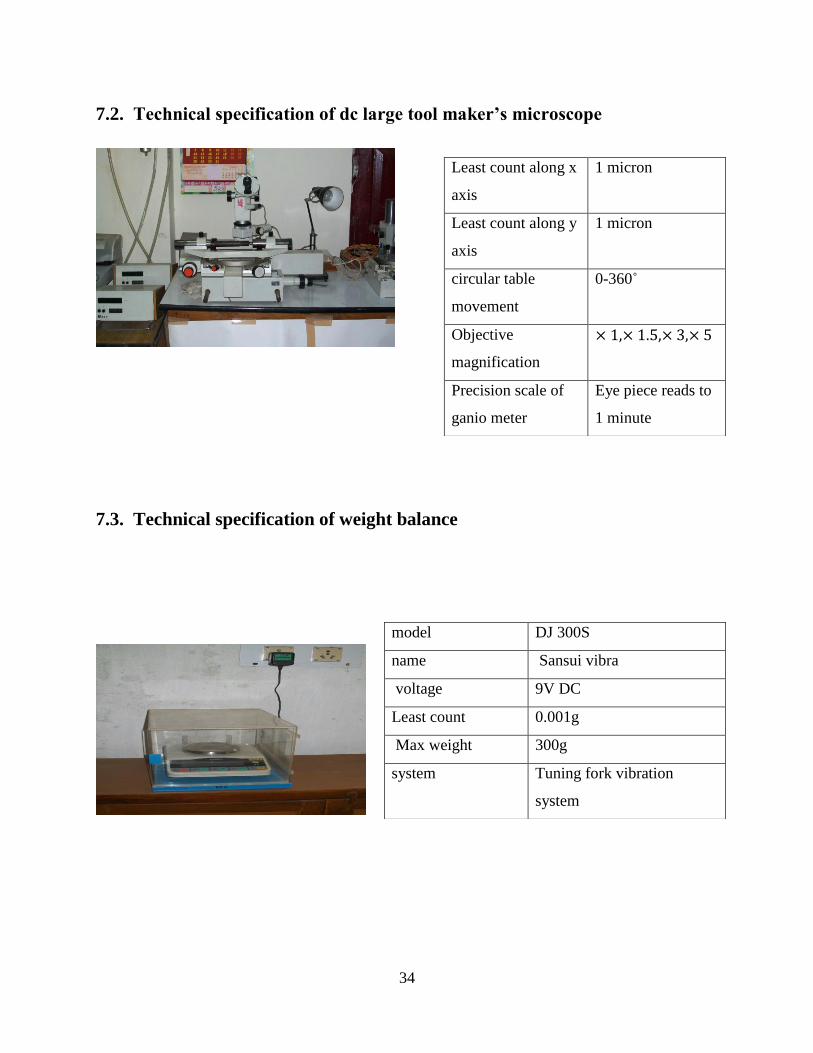
7.2. Technical specification of dc large tool maker’s microscope

7.3. Technical specification of weight balance

Least count along x

axis

1 micron

Least count along y

axis

1 micron

circular table

movement

0-360˚

Objective

magnification

Precision scale of

ganio meter

Eye piece reads to

1 minute

model DJ 300S

name Sansui vibra

voltage 9V DC

Least count 0.001g

Max weight 300g

system Tuning fork vibration

system

35

7.4 Technical specification of ECM machine setup

7.5 Technical specification of ECM control panel

Job holder.

100mm opening x 50mm depth x

100 width.

Tool feed motor Servo type

Cross head stroke 150mm

Electrical output rating 0-300amps at any voltage

between 0-20V

Operation mode Automatic/manual

timer 0-99.9 minutes

Tool feed rate 0.2-2 mm/min

Electrical supply 415V , 3 phase AC ,50HZ

Z axis control Forward, reverse by

microcontroller

36

REFERENCE

[1] NPTEL, IIT KHARAGPUR(LM 38)

[2] Heisch T., Mittemeijer E., Schultze J.W., “Electrochemical Machining Of Steel

100Cr6 in aqueous Nacl and NaNO3 solutions:microstructure of surface films

formed by carbides”-electrochimica acta 47(2001) 235-241

[3] Bhattacharyya B.,Munda J. “experimental investigation on the influence of

electrochemical machining parameters on machining rate and accuracy in

micromachining domain”.international journal of machine tools manufacture

43(2003) 1301-1310.

[4] Chakradhar D.,Venu Gopal A. “multi-objective optimization of

electrochemical machining of EN 31 steel by grey relational analysis”

international journal of modeling and optimization,vol 1,no.2,june 2011.

[5] Senthikumar C.,Ganesan G.,Karthikeyan R. “study of electrochemical

machining characteristics of Al/SiCp composites” int J manuf

technol(2009)43:256-263.

[6] João cirilo da Silva, Evaldo Malaquias da Silva, Marcio Bacci da silva

“Intervening Variables In Electrochemical Machining” journal of materials

processing technology 179(2006) 92-96

[7] Zhu D, Shu H.Y. “Improvement Of Electrochemical Machining Accuracy By

Using Dual Pole Tool” jaurnal of materials processing 129(2002) 15-18

[8] Honcheng H., Sun Y.H., Lin S.C.,Kao P.S. “A material removal analysis of

electrochemical machining using flat end cathode” journal of mterials

processing technology 140 (2003) 264-268