Optimisation of the Flow Process in Engine Bays - 3D...
144
THESIS FOR THE DEGREE OF DOCTOR OF PHILOSOPHY Optimisation of the Flow Process in Engine Bays - 3D Modelling of Cooling Airflow Peter V. Gullberg Department of Applied Mechanics CHALMERS UNIVERSITY OF TECHNOLOGY G¨ oteborg, Sweden, 2011
Transcript of Optimisation of the Flow Process in Engine Bays - 3D...

THESIS FOR THE DEGREE OF DOCTOR OF PHILOSOPHY
Optimisation of the Flow Process
in Engine Bays -
3D Modelling of Cooling Airflow
Peter V. Gullberg
Department of Applied MechanicsCHALMERS UNIVERSITY OF TECHNOLOGY
Goteborg, Sweden, 2011

Optimisation of the Flow Process in Engine Bays -3D Modelling of Cooling Airflow
PETER V. GULLBERGISBN 978-91-7385-559-4
c©Peter V. Gullberg, 2011
Doktorsavhandlingar vid Chalmers Tekniska hogskolaNy Serie nr 3240ISSN: 0346-718X
Department of Applied MechanicsChalmers University of TechnologySE-412 96 GoteborgSwedenTelephone +46 (0)31-772 1000
Cover:The flow process in the engine bay of a heavy duty truck.Illustrated by Martin Gullberg
This document was typeset using LATEX.
Chalmers ReproserviceGoteborg, Sweden 2011
Optimisation of the Flow Process in Engine Bays -
3D Modelling of Cooling Airflow
Peter V. GullbergDepartment of Applied MechanicsChalmers University of Technology
ABSTRACT
The focus of today’s automotive industry is to reduce emissionsand fuel consumption of all vehicles. Concentrating on the truckindustry, the last 20 years have focused largely on cutting emissionsof particulate matter and nitrogen oxides. For the future, attentionwill be on fuel consumption and emissions of carbon dioxide.
Significant changes have been made to fulfil new emission legis-lations, but the basic vehicle architecture has been kept. New aftertreatment systems that increases the thermal loading of the coolingsystem have been added within the same packaging envelope as be-fore. This means that there is less space to evacuate cooling airflowtoday and more airflow than ever is required.
Furthermore, project costs have increased over the years, focus isalso on cutting cost and lead times. Thus virtual development earlyin the project is highly desirable. Long before any prototypes areavailable, companies must now answer the question; will this truckhave competitive performance? As the project progresses, redesignsbecome more expensive. Development time is becoming more andmore limited, meaning any changes tend to become major changes.This has lead to a new focus of detailed and accurate simulations ofvehicle performance. For these reasons, in the context of underhoodthermal management, this project has been carried out; to improveand optimise the flow process in engine bays.
3D CFD supported by 1D models and measurements has beenstudied to predict the cooling airflow in the engine bay of trucks.The conclusions are that there are good opportunities to simulatethe flow process in engine bays early in development projects. Thisresearch project presents several different methods that, for differ-ent degrees of effort deliver different accuracy and indications arethat simulation can replicate measurements. This is though, withadvanced simulation models and a lot of computational effort, atleast seen from today’s perspective.
KEYWORDS: UTM, CFD, Cooling Airflow, Fans
iii

iv

ACKNOWLEDGMENT
Dear reader and receiver of this Thesis. This thesis will be the finalsign off, of my five year long PhD research project with the title;Optimisation of the Flow Process in Engine Bays. If it had not beenfor the invaluable support and work I received from a number ofpeople, this thesis would never had reached this level of completion.
I would like to thank Professor Lennart Lofdahl at ChalmersUniversity of Technology, Peter Nilsson and Lennart Eriksson atVolvo Trucks Corporation. Thank you for initiating this projectand laying a good foundation to what I am now presenting. Thankyou very much for your care and support during this time, and anespecially warm thank you to Lennart Eriksson for taking such goodcare of me during the first fragile months of my time as PhD-student.
At the university, I signed on at the same time asDavid Soderblomand Christoffer Landstrom. Lasse Christoffersen was already there.I owe you guys a lot. If it had not been for you, PhD would bea lot less like kindergarten and a lot more like prison. By takingpart in my project, you have made this journey joyful for me and Ithank you for that. If anyone is concerned about the use of the wordkindergarten, don’t be. I have been blessed with three very nice col-leagues at Chalmers. We have worked very hard together, pushingevery limit we could with regards to Chalmers facilities on subsonicisothermal fluid measurements and simulations. And at the sametime, more importantly we have had an incredible fun time doingthis. And this has meant a lot for me. You can definetly do seriouswork with a smile on your face. It has pushed me further, to takeon larger and more challenging tasks. After this, Jesper Marklund,Lisa Larsson, Helena Martini, Andrew Dawkes, Johnny Rice, andAlexey Vdovin joined the research group. Thank you guys for con-tributing. It has been very nice to get to know you, and I hope tocontinue to learn more from you. Andrew, thanks for helping mewith proper English.
v

A lot of my time I spent on Volvo Trucks. Thank you once morePeter Nilsson for letting me do this, and also for leaving me withplenty of Volvo’s resources at my disposal for this research project.I feel that I’ve had good support from Volvo with a very nice accessto the Fan Test Rig and the computational power at Volvo 3P.
At Volvo I’ve had the privelege of working with, Erik Dahl,Torbjorn Wiklund, Steven Adelman, Per Beckman, Mikael Englund,Kjell Andersson, Sassan Etemad, Erik Nordlander, Maria Krantz,Raja Sengupta, Jesper Axelsson, Andreas Lygner, Kaj Melin, PerKristedal, Katarina Jemt, Fredrik Bramer, Reimer Ryrholm, KurtNyblom, Anders Ottosson, Andreas Denneskog, Bjorn Andre andmany more. You have all taken part in this project by helpingme to understand the field of underhood thermal management, todevelop this field of research and what to focus on. I am glad tohave gotten the opportunity to get to know you and to cooperatewith you. Thank you.
Some special Thanks; Erik Dahl, I really do not know were tostart; What I think about most is that you challenge me not to usethe calculator all of the time, and instead use my head to do calculuswith. Most likely is that not what I should be most grateful about,and instead mention that you’ve taught me a lot about classicalfluid mechanics, thermodynamics, thermal management, 1D analy-sis, engineering methods and much more. I am certain that I needto learn more from you.
Torbjorn Wiklund, without a doubt, you have given me state ofthe art support with regards to any CFD problem I had.
Contributing to this project has also been a number of companies.To name some, CD-adapco with their office in London has supportedme with licenses for my simulations and support regarding CFDquestions, Robert Nyiredy, formerly at the Fluent Sweden office, forgeneral CFD support and Exa Corporation for support with LatticeBoltzmann. Kevin Horrigan is gratefully acknowledged for technicalcontributions.
I would also like to extend my gratitude to the Swedish EnergyAgency for funding this project.
Finally, I would like to thank my family and all of my friendsfor their warm and kind support. At the end of the day, you havealways been there for me. Thank You.
vi

LIST OF PUBLICATIONS
This thesis build upon research that was carried out at ChalmersUniversity of Technology between 2006 and 2009. The base of thethesis is presented in the following papers, referred to by Romannumerals in the text:
I Gullberg P., Lofdahl L., Tenstam A., Nilsson P., 3D Fan Mod-eling Strategies for Heavy Duty Vehicle Cooling Installations- CFD with Experimental Validation, FISITA World Automo-tive Congress 2008, Proceedings of FISITA World AutomotiveCongress, F2008-12-087, 2008. Main contributor: Gullberg P.
II Gullberg P., Lofdahl L., Adelman S., Nilsson P., A Correc-tion Method for Stationary Fan CFD MRF Models, SAE WorldCongress 2009, SAE Technical Paper 2009-01-0178, 2009. Maincontributor: Gullberg P.
III Gullberg P., Lofdahl L., Adelman S., Nilsson P., An Investi-gation and Correction Method of Stationary Fan CFD MRFSimulations, Thermal System Efficiencies Summit 2009, SAETechnical Paper 2009-01-3067, 2009. Main contributor: Gull-berg P.
IV Gullberg P., Lofdahl L., Adelman S., Nilsson P., ContinuedStudy of the Error and Consistency of Fan CFD MRF Models,SAE World Congress 2010, SAE Technical Paper 2010-01-0553,2010. Main contributor: Gullberg P.
V Gullberg P., Sengupta R., Axial Fan Performance Predictionsin CFD, Comparison of MRF and Sliding Mesh with Experi-ments, SAE World Congress 2011, SAE Technical Paper 2011-01-0652, 2011. Main contributor: Gullberg P.
VI Gullberg P., Lofdahl L., Axial Fan Modelling in CFD UsingRANS with MRF, Limitations and Consistency, a Comparison
vii
between Fans of Different Design Vehicle Thermal ManagementSystems 10 2011, Woodhead Publishing Limited C1305-009,2011. Main contributor: Gullberg P.
VII Gullberg P., Lofdahl L., Nilsson P., Fan Modeling in CFD UsingMRF Model for Under Hood Purposes, Proceedings of ASME-JSME-KSME Joint Fluids Engineering Conference 2011, AJKTechnical Paper AJK2011-23020, 2011. Main contributor: Gull-berg P.
VIII Gullberg P., Lofdahl L., Nilsson P., Cooling Airflow SystemModeling in CFD Using Assumption of Stationary Flow, Com-mercial Vehicle Engineering Congress 2011, SAE Technical Pa-per 2011-01-2182, 2011. Main contributor: Gullberg P.
viii

NOMENCLATURE
Scalar Quantities
d Diameter of fan [m]µ Viscosity of air [kg/s m]n Rotational speed [rpm]Pr Power [kW]p Pressure [Pa]qv Volumetric flow rate [m3/s]R Specific gas konstant [J/kg K]ρ Density of air [kg/m3]T Temperature [K]t Time [s]
Vector Quantities
r Position vector from rotating axis origin [m]uj Velocity vector [m/s]v Velocity vector [m/s]vr Velocity vector in rotating frame [m/s]ω Rotational vector [1/s]xj Coordinate vector [m]
Abbreviations
BFM Body Force MethodCAC Charge Air CoolerCAD Computer Aided DesignCFD Computational Fluid DynamicsCNC Computer Numerical ControlEGR Exhaust Gas RecirculationFPO Flat Plate Orifice
ix

Abbreviations
HVAC Heating, Ventilation and Air ConditioningLBM Lattice Boltzmann MethodLRF Local Reference FrameMRF Multiple/Moving Reference FramesOEM Original Equipment ManufacturerPDE Partial Differential EquationPM Particulate MatterRANS Reynolds Averaged Navier-StokesSLA StereolithographySM Sliding MeshSTL Stereolithography (CAD format)URANS Unsteady Reynolds Averaged Navier-StokesUTM Underhood Thermal Management
Definitions
bd Blade Depths
x
CONTENTS
1. Introduction . . . . . . . . . . . . . . . . . . . . . . . . . . 11.1 Background . . . . . . . . . . . . . . . . . . . . . . . 21.2 Purpose . . . . . . . . . . . . . . . . . . . . . . . . . 31.3 Scope . . . . . . . . . . . . . . . . . . . . . . . . . . 31.4 Underhood Thermal Management and the Cooling
Airflow Process . . . . . . . . . . . . . . . . . . . . . 41.4.1 Fuel Consumption and the Need for Cooling . 61.4.2 The Role of the Fan . . . . . . . . . . . . . . 61.4.3 The Need to Accurately Model the Fan and
the Cooling Airflow Process . . . . . . . . . . 7
2. Theory . . . . . . . . . . . . . . . . . . . . . . . . . . . . . 92.1 Experimental Measurements . . . . . . . . . . . . . . 9
2.1.1 Volvo 3P Fan Test Rig . . . . . . . . . . . . . 102.2 Numerical Simulations . . . . . . . . . . . . . . . . . 12
2.2.1 1D-models . . . . . . . . . . . . . . . . . . . . 122.2.2 3D-models . . . . . . . . . . . . . . . . . . . . 17
3. Preceding and Contemporary Work . . . . . . . . . . . . . 27
4. Overview of Technical Contributions . . . . . . . . . . . . 35
5. Isothermal Heat Exchanger Modelling . . . . . . . . . . . . 375.1 Method . . . . . . . . . . . . . . . . . . . . . . . . . 37
5.1.1 Experimental Measurements . . . . . . . . . . 405.1.2 Numerical Simulations . . . . . . . . . . . . . 40
5.2 Results and Discussion . . . . . . . . . . . . . . . . . 435.3 Intermediate Summary and Conclusions . . . . . . . 48
6. Fan Modelling . . . . . . . . . . . . . . . . . . . . . . . . . 516.1 Method . . . . . . . . . . . . . . . . . . . . . . . . . 51
xi

Contents Contents
6.1.1 Experimental Measurements . . . . . . . . . . 54
6.1.2 Numerical Simulations . . . . . . . . . . . . . 56
6.2 Results and Discussion . . . . . . . . . . . . . . . . . 65
6.2.1 Experimental Measurements . . . . . . . . . . 65
6.2.2 Numerical Simulations . . . . . . . . . . . . . 70
6.3 Intermediate Summary and Conclusions . . . . . . . 96
7. Isothermal Cooling Airflow System Modelling . . . . . . . 103
7.1 Method . . . . . . . . . . . . . . . . . . . . . . . . . 103
7.1.1 Experimental Measurements . . . . . . . . . . 103
7.1.2 Numerical Simulations . . . . . . . . . . . . . 105
7.2 Results and Discussion . . . . . . . . . . . . . . . . . 107
7.3 Intermediate Summary and Conclusions . . . . . . . 112
8. Summary . . . . . . . . . . . . . . . . . . . . . . . . . . . 115
9. Conclusions . . . . . . . . . . . . . . . . . . . . . . . . . . 117
10. Future Work . . . . . . . . . . . . . . . . . . . . . . . . . 119
11. Summary of Papers . . . . . . . . . . . . . . . . . . . . . . 121
Bibliography . . . . . . . . . . . . . . . . . . . . . . . . . . . 127
Paper I . . . . . . . . . . . . . . . . . . . . . . . . . . . . . . 131
Paper II . . . . . . . . . . . . . . . . . . . . . . . . . . . . . . 143
Paper III . . . . . . . . . . . . . . . . . . . . . . . . . . . . . 151
Paper IV . . . . . . . . . . . . . . . . . . . . . . . . . . . . . 165
Paper V . . . . . . . . . . . . . . . . . . . . . . . . . . . . . . 175
Paper VI . . . . . . . . . . . . . . . . . . . . . . . . . . . . . 193
Paper VII . . . . . . . . . . . . . . . . . . . . . . . . . . . . . 207
Paper VIII . . . . . . . . . . . . . . . . . . . . . . . . . . . . 221
xii

Contents Contents
Appendix 237
A. Theory Details . . . . . . . . . . . . . . . . . . . . . . . . 239A.1 Volvo 3P Fan Test Rig . . . . . . . . . . . . . . . . . 239A.2 3D-models . . . . . . . . . . . . . . . . . . . . . . . . 248
xiii


1. INTRODUCTION
Modern society faces big challenges with regards to individual mo-bility, goods transport and general energy supply. Our society hasflourished owing to the availability of cheap energy. Thanks to cheapcrude oil, coal and nuclear power, to mention some sources of en-ergy, we have become used to individual mobility; most of us haveaccess to one or two cars and with the infrastructure of moderncountries we can move us around as we want. We are also usedto the fact that goods, merchandise and consumables are cheapestbought if they are manufactured in China, Taiwan or any other de-veloping country. It is a very political question whether to considerChina as developing country or developed country, considering itssize and influence on the world trade market. More importantly,owing to cheap transportation, the fact that China is located onthe other side of the globe does not influences the trade of Chinesegoods in our part of the world to any large extent. Finally we arealso used to having electricity around to power our televisons, com-puters, washing machines and more. We are used to having electricenergy without spending a significant part of our monthly incomeon it to afford it.
Today everyone is aware of the fact that the price of oil is in-creasing. We are also looking into what effects emissions of fossilfuels might have on our environment and planet. Many initiativeshave been taken to reduce emissions of substrates that have, andcan have, a detrimental effect on our health and environment.
The automotive industry has always faced great challenges toovercome; customer demands, tough competition, legislation, latelyeconomic crisis and more. For the last ten years it has worked tire-lessly to reduce emission, to specifically mention the Heavy DutyDiesel industry, it has focused on reducing emissions of nitrogen ox-ides and particulate matter. Emissions legislation has been enforcedon both the US market, European and Japanese. Led by these mar-
1

1. INTRODUCTION
kets most of the other countries in the industrialised world have fol-lowed. Significant cuts have been made to reduce emissions throughskilled engineering and innovation.
For the future, the automotive industry, heavily dependant onfossil fuels, will face yet another challenge; how to develop, produceand sell sustainable mobility and sustainable transport services. Inorder for our society to transform from a society with detrimentaleffects upon our environment and planet, to a Sustainable Society.
For the future, put plainly, everyone within the automotive in-dustry is aware, that the focus will be on fuel consumption, carbondioxide emissions, vehicle energy management and energy storage.
1.1 Background
Although significant changes have been made to vehicles in orderto fulfil new emission levels, the basic vehicle architecture has re-mained. To reduce emissions, new exhaust gas after treatment sys-tems have been added. Engine management systems have increasedin size and complexity and all of this is done within the same vehicleenvelope as before. This has meant two things for the design field ofunderhood thermal management; engine thermal management con-straints have increased, the new engines need to be maintained withincreased precision to become more efficient, and there has been alot more components added to the engine bay, so that, evacuatingthe hot air out of the engine bay has become more of a critical mat-ter. Today we have less space to evacuate cooling airflow, plus weneed more airflow than ever since the heat rejection from the engineincreases.
Connected to the problem is also the fact that most compete-tive automotive OEM’s focus heavily on cutting project lead times.Projects tend to become larger and more expensive and thereforecutting the project time is a way of cutting cost and also to reducethe pay back time of the investment.
Consequently there is great need for virtual development andvirtual performance testing early in new automotive projects. Typ-ically long before any ”mules” or prototypes are available, compa-nies must now answer the question; Will this truck have competi-tive performance? Also typically as a project develops it becomesmore expensive to carry out any re-designs. Since everything is now
2

1.2. PURPOSE
so tightly packaged together, any changes tend to become majorchanges and major changes are expensive.
This has lead to a new focus of very detailed and accurate simu-lations of vehicle performance early in project phases. For these rea-sons, in the context of underhood thermal management, this projecthas been carried out; to improve and optimise the flow process inengine bays.
1.2 Purpose
The title of this research project is Optimisation of the Flow Processin Engine Bays and the scope of it is to improve the design processof underhood thermal management with a specific focus on coolingairflow. The purpose is to develop and evaluate engineering methodsof simulating the cooling airflow in a truck engine bay environment.The focus is not only on absolute accuracy, but also different levelsof accuracy. Taking into account the fact that, absolute accuracyis not always required in a project. In some phases, this constraintcan be relaxed in order to acquire results faster.
This thesis will present different modelling strategies for the cool-ing airflow using 3D CFD, supported by 1D models and measure-ments. The level of accuracy of different modelling strategies arejudged through direct comparison with experimental testing, per-formed in all cases on an, as near as possible, identical set-up ofgeometry.
1.3 Scope
For this thesis some limits are set. This thesis will only focus oncooling airflow from the standpoint of isothermal flow. There willbe no sources of heat put into either simulations nor measurements.Furthermore heat exchangers in the cooling airflow channel will onlybe modelled in a lumped format. No detailed fin or tube structurewill be accounted for. Finally this thesis will be heavily focused onheavy duty truck cooling installation. However many conclusionsand much of the information presented will be valid and of interestfor the rest of the automotive industry.
3
1. INTRODUCTION
1.4 Underhood Thermal Management and the Cooling Airflow
Process
This section will put this thesis into its technical context withinunderhood thermal management development.
Underhood Thermal Management (UTM) covers the engineeringfield of solutions that maintains the complete vehicle powertrain inacceptable ranges of operation with regards to component and fluidtemperatures. The diesel engine of today is the most efficient com-bustion engine available. Maximum efficiency ratings today reachesup to 45%. Since this is not 100% and engine ratings on truckstoday are high, a vast amount of waste energy in the form of heatis created. This heat is partly ejected in the exhausts and partlytransmitted to the engine cooling circuit.
UTM covers multiple subsystems, some of them are listed belowand elaborated:
• Cooling down and heating up the engine coolant system. Cool-ing down to control combustion temperatures and keep the en-gine from overheating and by that maintaining or improvingthe expected life. Heating the water system up to avoid exces-sive friction caused by cold engine lubricants.
• Charge air cooling which involves keeping the air inlet tem-peratures into the engine down and by this increasing engineefficiency significantly.
• Transmission cooling, to prevent overheating of transmissionoil. Overheating the oil quickly degrades it.
• Air conditioning condenser cooling, dissipate the absorbed heatfrom the air conditioning system.
• Exhaust gas recirculation cooling, to cool down exhaust gasesif these are needed to recirculate into the combustion chambereither for improved efficiency or better emissions control
• Compressed air cooling, if the truck is equipped with an airsystem for braking or suspension, compressing this air gener-ates heat, and temperatures must be controlled to prevent theair drying system degrading.
4
1.4. UNDERHOOD THERMAL MANAGEMENT AND THE COOLINGAIRFLOW PROCESS
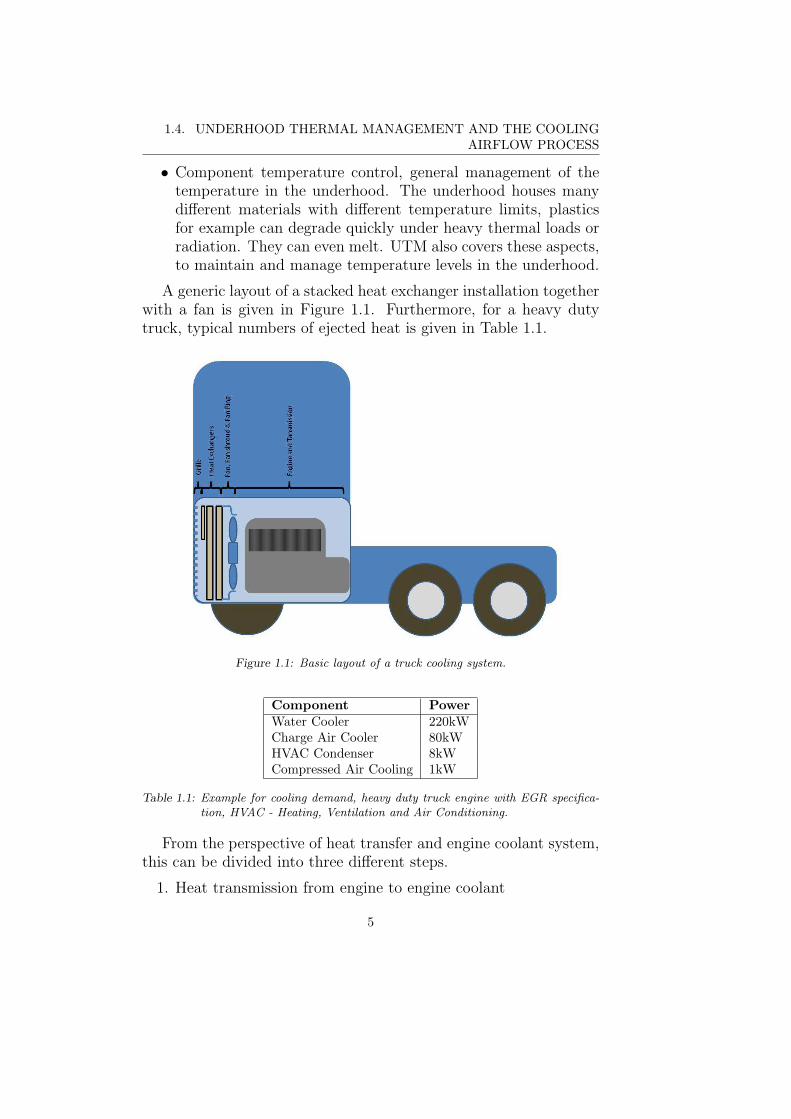
• Component temperature control, general management of thetemperature in the underhood. The underhood houses manydifferent materials with different temperature limits, plasticsfor example can degrade quickly under heavy thermal loads orradiation. They can even melt. UTM also covers these aspects,to maintain and manage temperature levels in the underhood.
A generic layout of a stacked heat exchanger installation togetherwith a fan is given in Figure 1.1. Furthermore, for a heavy dutytruck, typical numbers of ejected heat is given in Table 1.1.
Figure 1.1: Basic layout of a truck cooling system.
Component PowerWater Cooler 220kWCharge Air Cooler 80kWHVAC Condenser 8kWCompressed Air Cooling 1kW
Table 1.1: Example for cooling demand, heavy duty truck engine with EGR specifica-tion, HVAC - Heating, Ventilation and Air Conditioning.
From the perspective of heat transfer and engine coolant system,this can be divided into three different steps.
1. Heat transmission from engine to engine coolant
5

1. INTRODUCTION
2. Engine Coolant Circuit, that transports the heat from the en-gine to the heat exchangers
3. Dissipation of heat from the hot coolant into the ambient airthrough forced convection
Similar divisions can be made for the other subsystems. Thisthesis, as outlined in Section 1.3, will only deal with the third stepwhich is the cooling airflow side of UTM.
1.4.1 Fuel Consumption and the Need for Cooling
For fuel consumption it is of course important to have efficient en-gines, but additionally it is important to use the available power inan efficient way. In this context the cooling system plays two roles.The first and major role is that it is necessary for making fuel effi-cient engines as explained above. The second part in this contextis that the cooling systems constitutes a loss. Typically one hasa significant pressure drop over the heat exchanger in the airflowcooling circuit, the fan that drives the airflow consumes power, evenso the airflow through the cooling system increases the overall aero-dynamic drag of the vehicle. So to design fuel efficient vehicles, thesubsystem of cooling needs to be designed efficiently with as littlelosses as possible.
1.4.2 The Role of the Fan
The cooling fan is the main driver of cooling airflow in the under-hood. And this component has become a critical feature in currentheavy duty cooling systems, it is needed to fulfil the demand of en-gine cooling but its power consumption is in no way negligible, fullyengaged it typically consumes of the order of magnitude 50hp. In ad-dition to this it also emits unwanted noise which is starting to causelegislative compliance problems for automotive OEMs. The noiselevel from a fully engaged fan can well be of an order of magnitude100-110 dB. Furthermore, future engine systems will demand morecooling. Increasing the airflow through the engine bay by installinga stronger fan serves as a cost effective way of at least partiallyachieving this goal.
Thus there is a significant need to understand the fan and its in-teraction with other components in the engine bay. This is required
6
1.4. UNDERHOOD THERMAL MANAGEMENT AND THE COOLINGAIRFLOW PROCESS
in order to fulfil the demand for more cooling airflow with less powerconsumption.
1.4.3 The Need to Accurately Model the Fan and the Cooling
Airflow Process
As the lead times of vehicle development are decreasing, it is de-sirable to perform better predictions of the actual performance ofthe complete vehicle earlier in the development process. Historicallyvehicle cooling systems development was carried out with substan-tially complete vehicles late in the development process. This can nolonger satisfy the need for faster, cheaper and more efficient develop-ment processes, and in this context 3D CFD simulation capabilitiesoffers great potential to fulfil this demand.
In order for the transition of this process from classical develop-ment using substantial amounts of physical testing to modern tech-niques using numerical simulations, one must have at one’s disposalgood tools and models to simulate the components and systems onewants to develop.
In this context, of underhood thermal management, one needsgood models of the heat exchangers, fan, and airflow in the enginebay.
In this thesis focus is on how to model the cooling airflow using3D CFD in an accurate, fast and efficient manner.
7

1. INTRODUCTION
8

2. THEORY
The focus of this thesis has been to use experimental measurementstogether with 1D simulation methods to support the task of validat-ing different 3D CFD modelling techniques, in the context of enginebay cooling airflow. For the purpose of understanding the underlyingtheory behind simulations and measurements this chapter, togetherwith the support of the appendix, will explain the details of theengineering tools used for this thesis and research project.
2.1 Experimental Measurements
For the experimental measurement and testing part of this projectthe Volvo 3P Fan Test Rig was used. This rig is a plenum to plenumclosed loop type of test rig, where the outlet chamber is maintainedat ambient pressure. An artistic presentation of the Fan Test Rig isdepicted in Figure 2.1.
Figure 2.1: Artistic representation of the Volvo 3P Fan Test Rig.
9

2. THEORY
2.1.1 Volvo 3P Fan Test Rig
A more detailed plan view of the test rig is given in Figure 2.2. Re-ferring to this figure, the return circuit (1) at A, shows the mainfan drive. This is a 2-speed 90kW electric motor and blower, andit is the main driver of airflow through the rig. This unit draws airthrough a flow regulator (B) which in turn is connected to a settlingchamber (C) and the airflow measuring nozzles (D). The settlingchamber smooths out and stabilises the flow to the pressure cham-ber. The airflow measuring nozzles are a set of 6 venturi type nozzles(ISA 1932) which are used to measure the air mass flow through therig. These are explained in greater detail in Appendix A.1 Nozzlesand Volumetric Flow Measuring. By disengaging the main fan andonly controlling the flow regulator (B) a flow restriction in the rigcan be simulated.
Figure 2.2: Detailed plan view of the Volvo 3P Fan Test Rig, fan testing set-up.
The main fan drive supplies air down to the Pressure Chamber(2). This is through a set of stator vanes to regain some of the dy-namic pressure and also even out the flow field. The pressure cham-ber is divided into two sections, separated by a flow straighteninggrid (E). This grid straightens and uniformly distributes the flowin the pressure chamber. The static pressure in the pressure cham-ber is measured in a shielded compartment at location (a). With
10

2.1. EXPERIMENTAL MEASUREMENTS
this controlling the pressure chamber has an operating pressure of±5000 Pa or a max airflow at zero pressure of 18m3/s is possible.The temperature in the pressure chamber is monitored in four posi-tions on the straightening grid. The temperature is measured withpt100 sensors.
The air in the pressure chamber is then guided towards the testobject (F ) which is located between the the pressure chamber (2)and the outlet chamber (3). The test object is placed at F , whichin these tests is typically the cooling installation with different lev-els of detail together with a cooling fan. Connected to the fan isa 75kW DC-motor (G) driving the fan and it has a max speed of2977rpm. Details about this motor and measuring the fan torque isgiven in Appendix A.1Measuring Fan Power. The outlet chamber ismaintained at ambient pressure and reference parameters are moni-tored at location b. Outside the test rig atmospheric parameters aremeasured; temperature, barometric pressure and air moisture levels.
The airflow out of the outlet chamber is guided back to the re-turn circuit (1) through a set of heat exchangers (H). These heatexchangers serves to keep the temperature in the inlet chamber con-stant. At maximum airflow rate the maximum performance for theseheat exchangers is to cool 65oC air to 25oC.
For the interested reader, the Fan Test Rig is explained furtherin Appendix A.1. This appendix deals with Measuring Fan Power,Nozzles and Volumetric Flow Measuring, transforming measuredquantites to standard air conditions (Standard Air Conditions), theaccuracy of the test rig (Accuracy) and some further definitions ofthe test rig (Definitions).
Velocity Measurements across Radiator
Additionally for this thesis a pressure scanning system was usedto measure the air velocity distribution across the heat exchanger.The working principle behind the system is simple. The radiatoris fitted with 48 micro probes, these probes are installed betweentwo tubes and two fins in the radiator in 48 different positions. Theprobe has the same principle as a pitot tube and with a differentialpressure transducer the dynamic pressure is measured. A scanivalvesystem is located before the transducer to control and manage the48 different probes.
11

2. THEORY
Installing the probes in a radiator in a test rig for a test condi-tion that allows for completely uniform airflow through the radiator,the probes can be calibrated. Calibration is performed by sweepingdifferent flow rates through the test rig, monitoring the flow rate,converting it to radiator velocity assuming uniform flow, and thenmonitoring the signal from the pressure transducer. By this proce-dure the probe signal is calibrated to the local air velocity throughthe radiator. Some further details of the theory behind the systemis given in Appendix A.1 Velocity Measurements across Radiator.
The specific system used for this thesis was developed by RuijsinkDynamic Engineering. Some further details are found athttp://www.ruijsink.nl/rde-mpr.htm and additionally the system isused for research purposes in [10].
2.2 Numerical Simulations
2.2.1 1D-models
Classically, modelling and predicting the airflow through an enginebay has been done in what can be considered as 1-dimensional mod-els.
The classical approach in these models is to predict the pressurerise or drop in the different components in the cooling system, suchas fan and radiator. The pressure rise or drop is predicted overdifferent mass flow rates of air, or volumetric flow rate, and thenthis model is put together to predict a simplified characteristics ofthe system.
The main drivers of flow through the cooling system are the fanand ram air (dynamic pressure governed by the vehicle operatingspeed). The main restrictors in the system are the pressure dropthrough the heat exchangers and the built-in restriction (pressuredrop in the engine bay due to bluff geometry).
For a set volumetric flow rate, vehicle- and fan speed, this canbe illustrated as Figure 2.3. In Figure 2.3 there are two curves.The blue one represents a common dimensioning criteria, full loadand low speed driving. Characterising this drive mode is a highdemand for airflow through the heat exchangers, hence there is ahigh pressure drop in these components (3). Due to the low speedof driving there is little access to ram air pressure rise (seen by a
12

2.2. NUMERICAL SIMULATIONS
Figure 2.3: Trace of static pressure through an engine bay.
small contribution from ram air (1)), so to overcome the pressuredrop in the heat exchangers the fan is fully engaged and the majordriver of airflow (5).
The red curve in Figure 2.3 represents a light load cruise condi-tion. Here, there is more access to ram air, and there is no significantneed of cooling, hence the fan does not need to engage to any greatextent.
The model used as a base in this thesis was proposed by Dav-enport [8] in 1974. Recently, work has been done on this model byCowell [9].
This model has the form of Equation (2.1).
∆pF = ∆pR +∆pSys +1
2ρv2F − 1
2Fρv20 (2.1)
In this equation the notation in Table 2.1 apply.
Term Explanation∆pF Fan Pressure Rise∆pR Radiator or Cooling Package Pressure Drop∆pSys System Restriction1
2ρv2F Fan Dynamic Head
1
2Fρv2
0Ram Air Pressure, F is ram air effectiveness
Table 2.1: Local nomenclature to Equation (2.1).
13

2. THEORY
What is required in this model is the air velocity through the ra-diator, since it determines available cooling air. Hence one expressesthe pressure drops and rises in the above equation as functions ofair velocity or mass flow and applies mass conservation to connectthe velocities in different stages of the system. The different com-ponents in this equation, Equation (2.1), will be explained in latersections. A very common approach to Equation (2.1) is to combine∆pSys and 1
2ρv2F into one system restriction term. Furthermore de-
pending on the problem and the purpose of the problem, differentterms can be extracted and identified from ∆pR or ∆pSys. An exam-ple of this is a stacked heat exchanger where one can split out eachseparate module and identify the separate contributions to pressuredrop. Also a widepread practice is to take out different accelerationlosses or exit losses from the system restriction term.
Defining any exact theoretical descriptions of these pressure dropsis very difficult, and the closest currently achievable is 3D CFD,discussed later, however this has not always been so precise. Tra-ditionally simpler empirical models of these components have beenbuilt based on measured data. This will be discussed in the comingsubsections.
Fan Curves
To get ∆pF in Equation (2.1) one needs to measure what is com-monly known as the ”fan curve”. A fan curve is typically charac-terised by measuring the fan pressure rise for different volumetricflow rates at a set fan rotation speed. Measuring this in a plenum toplenum fan test rig, such as the one described in Section 2.1, resultssimilar to Figure 2.4 are typical. In Figure 2.4 the static efficiencyfor the fan is plotted, defined by Equation (A.15).
For plenum to plenum test conditions this is the characteristiccurve one gets for an axial fan that is used in todays heavy duty truckcooling installations. It consists of two regions, referenced as; axialdomain and diagonal/radial domain in Figure 2.4. Between theseregions there is a transition region, this region is also sometimesreferred to as fan stalling region, and is unstable in nature.
Other types of test set-ups such as duct to duct testing or a tubu-lar test facility (in essence test facilities with different inlet and exitgeometry to the test object) generate slightly different characteris-
14

2.2. NUMERICAL SIMULATIONS
Figure 2.4: Typical fan curve.
tics for the same fan, especially in the sensitive transition region.These will, in this thesis, not be discussed any further, since theplenum to plenum test is the industry standard.
When it comes to building an empirical fan model from a mea-sured fan curve, Cowell [9] suggests estimating these curves witha parabola. Doing this estimation one will not include the strongeffect of the transition of these types of fans, since a parabola is ofsecond order. To capture this one would need at least a third ordermethod. This is also commented in Cowell’s paper.
The other alternative is to interpolate a curve between the mea-sured points and iteratively solve Equation (2.1). This is argued bythe author of this thesis to be the most appropriate method.
Fan Laws
For an individual fan, various rules have been derived and provedto apply, see Equations (2.2 - 2.4) these are typically known as thefan laws. Similarly these laws apply for pumps, however in thisfield they are known as pump laws. If a fan curve or pump curvehas been measured for a specific speed, diameter and density, theselaws can theoretically be used to calculate the fan curve for anyother speed, diameter or density. Practically these laws have some
15
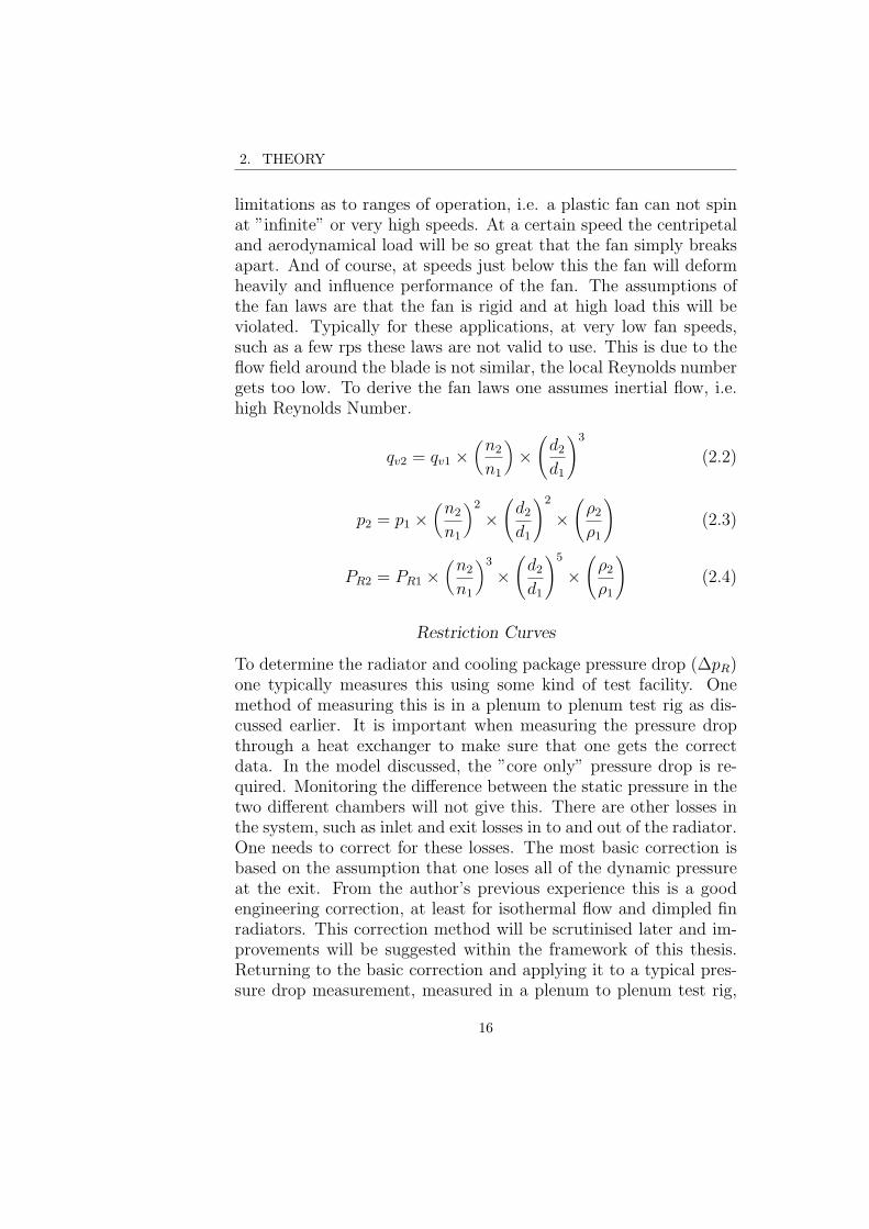
2. THEORY
limitations as to ranges of operation, i.e. a plastic fan can not spinat ”infinite” or very high speeds. At a certain speed the centripetaland aerodynamical load will be so great that the fan simply breaksapart. And of course, at speeds just below this the fan will deformheavily and influence performance of the fan. The assumptions ofthe fan laws are that the fan is rigid and at high load this will beviolated. Typically for these applications, at very low fan speeds,such as a few rps these laws are not valid to use. This is due to theflow field around the blade is not similar, the local Reynolds numbergets too low. To derive the fan laws one assumes inertial flow, i.e.high Reynolds Number.
qv2 = qv1 ×(n2
n1
)
×(
d2d1
)3
(2.2)
p2 = p1 ×(n2
n1
)2
×(
d2d1
)2
×(
ρ2ρ1
)
(2.3)
PR2 = PR1 ×(n2
n1
)3
×(
d2d1
)5
×(
ρ2ρ1
)
(2.4)
Restriction Curves
To determine the radiator and cooling package pressure drop (∆pR)one typically measures this using some kind of test facility. Onemethod of measuring this is in a plenum to plenum test rig as dis-cussed earlier. It is important when measuring the pressure dropthrough a heat exchanger to make sure that one gets the correctdata. In the model discussed, the ”core only” pressure drop is re-quired. Monitoring the difference between the static pressure in thetwo different chambers will not give this. There are other losses inthe system, such as inlet and exit losses in to and out of the radiator.One needs to correct for these losses. The most basic correction isbased on the assumption that one loses all of the dynamic pressureat the exit. From the author’s previous experience this is a goodengineering correction, at least for isothermal flow and dimpled finradiators. This correction method will be scrutinised later and im-provements will be suggested within the framework of this thesis.Returning to the basic correction and applying it to a typical pres-sure drop measurement, measured in a plenum to plenum test rig,
16
2.2. NUMERICAL SIMULATIONS
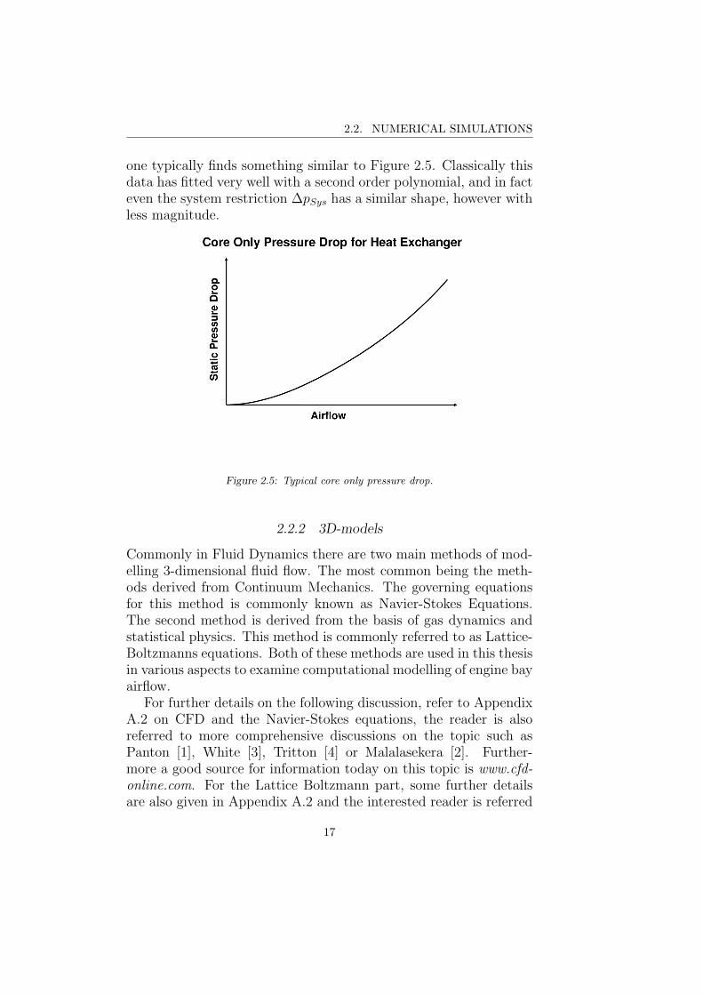
one typically finds something similar to Figure 2.5. Classically thisdata has fitted very well with a second order polynomial, and in facteven the system restriction ∆pSys has a similar shape, however withless magnitude.
Figure 2.5: Typical core only pressure drop.
2.2.2 3D-models
Commonly in Fluid Dynamics there are two main methods of mod-elling 3-dimensional fluid flow. The most common being the meth-ods derived from Continuum Mechanics. The governing equationsfor this method is commonly known as Navier-Stokes Equations.The second method is derived from the basis of gas dynamics andstatistical physics. This method is commonly referred to as Lattice-Boltzmanns equations. Both of these methods are used in this thesisin various aspects to examine computational modelling of engine bayairflow.
For further details on the following discussion, refer to AppendixA.2 on CFD and the Navier-Stokes equations, the reader is alsoreferred to more comprehensive discussions on the topic such asPanton [1], White [3], Tritton [4] or Malalasekera [2]. Further-more a good source for information today on this topic is www.cfd-online.com. For the Lattice Boltzmann part, some further detailsare also given in Appendix A.2 and the interested reader is referred
17

2. THEORY
to more comprehensive literature on the topic such as Succi [5] orthe work presented by Guo et.al. in [11].
Navier-Stokes Equations
There are three equations governing fluid dynamics in the Navier-Stokes approach. These are three conservation laws, conservation ofmass (Equation (2.5)), conservation of momentum (Equation (2.6))and conservation of energy (Equation (2.7)).
∂ρ
∂t+
∂
∂xj
(ρuj) = sm (2.5)
∂
∂t(ρui) +
∂
∂xj
(ρuiuj + pδij − τji) = si, i = 1, 2, 3 (2.6)
∂
∂t(ρe0) +
∂
∂xj
(ρuje0 + ujp+ qj − uiτij) = se (2.7)
What each term on the left hand side in the above equationsmeans is further elaborated in Appendix A.2. Furthermore in Ap-pendix A.2 details are given on boundary conditions to a set prob-lem, simplifying assumptions such as incompressible and isothermalflow and how to progress from the above equations to the ReynoldsAveraged Navier-Stokes (RANS) equations. The RANS equationsare the formulation for fluid flow today, in all steady state commer-cial CFD codes. In Appendix A.2 the formulation of each turbulencemodel used in later investigation is also given, and finally some de-tails are given on how to discretise all of these equations.
The terms on the right hand side in Equations (2.5 - 2.7) aresource terms that are used to model different aspects of non-standardisedfluid flow phenomenas, such as sinks or sources. These will be usedin certain aspects of this thesis, amongst them, modelling the heatexchanger pressure drop.
Porous Media
To model a heat exchanger, or more specifically the radiator, for aproblem of this size, the assumption of porous media is commonlyused. A porous media model incorporates empirically determinedflow resistance in the domain of the model defined as porous. Inessence porous media is a momentum sink in the governing equations
18

2.2. NUMERICAL SIMULATIONS
that corresponds to the empirically measured flow resistance, thatis the curve measured in Figure 2.5
Porous media are modelled with the addition of a momentumsource term (si) in standard Navier-Stokes equations, Equation (2.6).The momentum source term is composed of a viscous loss term (lin-ear) and an inertial loss term (quadratic). Typically it is presentedas Equation (2.8). Here Pv is the constant viscous resistance coeffi-cient matrix, Pi is the inertial resistance matrix coefficient. Equation(2.8) is commonly known as Darcy-Forchheimer’s law.
si = − (Pvµ · v + Piρ |v| · v) (2.8)
This momentum sink contributes to the pressure gradient in theporous cell, creating pressure drop that is proportional to the fluidvelocity, or velocity squared in the cell.
Fan Models
Within commercial software currently available, there are three mainmodels for simulating the fan. These are;
1. Momentum Source Methods: This method is sometimes alsoreferred to as Body Force Method (BFM) and employs an ”ac-tuator disk” type of implementation. In this method, the de-tailed fan geometry is not presented physically, but its momen-tum contributions are handled with volume source terms thatare inserted into the transport equations (si in Equation (2.6))in the cells swept by the blades. This model uses a specifiedfan curve, such as described in Section 2.2.1 Fan Curves. A fancurve is presented as static pressure rise over volume flow ratefor a specific temperature and rotational speed. From the fancurve one can derive volume forces to these cells for a specifiedtemperature and rotational speed. For these derivations themomentum source method uses the the fan laws, which wasdiscussed in Section 2.2.1 Fan Laws. A schematic figure of thismethod is displayed in Figure 2.6.
There are two big drawbacks with this method. The first oneis that this method typically requires a substantial mappingeffort of the fan that will be used in the simulated system: oneneed the measured fan curve. This poses some severe restric-tions, first of all this model cannot be used to develop fans.
19

2. THEORY
Figure 2.6: The principle behind the momentum source method. The pressure balancethat applies is Phigh = Plow + Prise where Prise is given from input datafrom the fan curve.
Furthermore one become severely limited to develop anythingthat has an interaction with the fan performance, such as fanrings, diffusers and guide vanes. Secondly, this model does nottake into account the swirl being produced by the rotating fan.This has the effect that the correct amount of energy is notbeing fed into the underhood during simulations. Some com-mercial software allows for source terms corresponding to swirland radial flow, but usually this does not help the engineersince these contributions are commonly not measured duringfan testing. Additionally one can estimate these contributions,but this is not very common.
2. Frozen Rotor Simulations: This model uses the geometrical pre-sentation of the fan. Momentum and turbulence contributionsfrom the fan are modelled via a technique referred to as Mov-ing Reference Frames (MRF). Using this method, the rotationis not modelled explicitly, but source terms stem from the re-formulation of the transport equations into a rotating frame ofreference. This is done for a control volume that encompassesthe fan geometry. Hence the nature of the simulation is steadystate, and information about any flow features varying in timewill be lost.
20

2.2. NUMERICAL SIMULATIONS
To use this model one separates the fluid region into rotatingand non-rotating regions. In non-rotating regions the regulargoverning equations are solved; and in rotating regions the gov-erning equations are transformed into a rotating frame of refer-ence using Equation (2.9). A schematic figure of the principleof this method is shown in Figure 2.7.
v = vr + ω × r (2.9)
Figure 2.7: The principle behind the MRF method. The pressure balance that appliesis Phigh = Plow + Prise where Prise is given from the actual mathematicalrotation of the volume encompassing the fan.
Doing this transformation, Equation (2.9), in the rotating frameadds centripetal and Coriolis acceleration to the momentumequations. Across the interface between the different regions alocal reference frame transformation is performed to allow forflux calculations. For standard MRF, local continuity is en-forced across, scalar quantities such as temperature, pressure,density etc. are just passed on over the interface locally. Vec-torial quantities such as velocity v are transformed over theinterface with ω, according to Equation (2.9).
In each separate frame, the physics is correctly formulated andthe simplest use of this method is using a single reference frame.This allows rotating objects to be of any shape. The main lim-itation is for non-rotating objects, these need to be surfaces of
21
2. THEORY
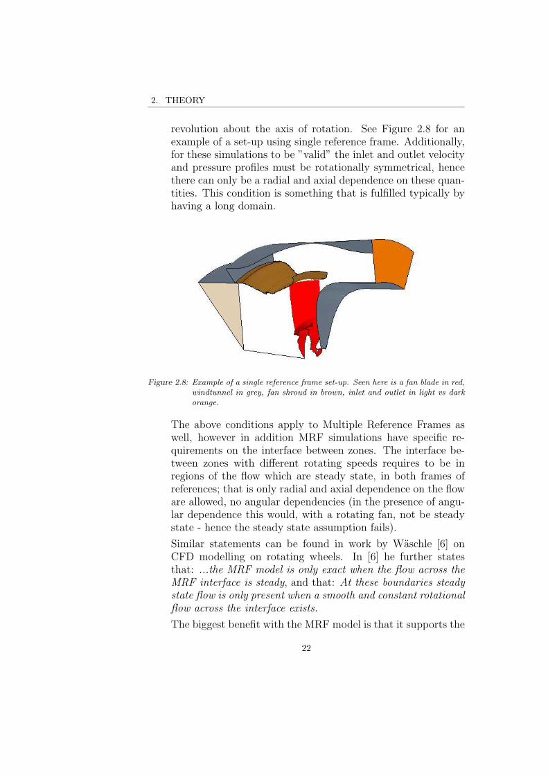
revolution about the axis of rotation. See Figure 2.8 for anexample of a set-up using single reference frame. Additionally,for these simulations to be ”valid” the inlet and outlet velocityand pressure profiles must be rotationally symmetrical, hencethere can only be a radial and axial dependence on these quan-tities. This condition is something that is fulfilled typically byhaving a long domain.
Figure 2.8: Example of a single reference frame set-up. Seen here is a fan blade in red,windtunnel in grey, fan shroud in brown, inlet and outlet in light vs darkorange.
The above conditions apply to Multiple Reference Frames aswell, however in addition MRF simulations have specific re-quirements on the interface between zones. The interface be-tween zones with different rotating speeds requires to be inregions of the flow which are steady state, in both frames ofreferences; that is only radial and axial dependence on the floware allowed, no angular dependencies (in the presence of angu-lar dependence this would, with a rotating fan, not be steadystate - hence the steady state assumption fails).
Similar statements can be found in work by Waschle [6] onCFD modelling on rotating wheels. In [6] he further statesthat: ...the MRF model is only exact when the flow across theMRF interface is steady, and that: At these boundaries steadystate flow is only present when a smooth and constant rotationalflow across the interface exists.
The biggest benefit with the MRF model is that it supports the
22

2.2. NUMERICAL SIMULATIONS
steady state formulation of fluid flow but still uses the geomet-rical representation of the fan. This means it is not dependenton experimental data. Since it is mathematically correct underthe condition that the steady state assumption across the in-terface applies and makes sense, this model simulates swirl andradial acceleration. The biggest drawback though, is that formost cases it is impossible to fulfil the steady state assumption.This model will however, not produce a divergent solution, itis in this sense robust, but it will produce erroneous results.
An important factor about this model as well is that; since itis commonly not possible to fit a valid rotational region aroundthe fan in most simulations, this model will produce erroneousresults, however the choice of rotational region will affect the er-ror. There are two common choices of regions; One is a cylinderencompassing the fan, as indicated in Figure 2.7. The advan-tage of this choice is that this type of simulation can be easilyconverted into the next type of fan simulation: Rigid Body Ro-tation. The second choice of region is one that is grown outto the fan ring. With this method one places the fan ring incounter-rotation to the rotating domain (in this way it is sta-tionary in the master coordinate system). The big benefit withthis method is that one avoids the blade tip overflow going outof the MRF region from the pressure side of the blade and goingin again at the suction side of the blade. This will violate theMRF steady state requirement for validity and produce errors.The drawback though is that generally most fan rings and fanshrouds are not radially symmetric, hence this will also produceerrors with non-rotationally symmetrical MRF regions.
3. Rigid Body Rotation: In this model the fan geometry is fullydetailed and the momentum and turbulence contributions aremodelled through the actual rotation of the part of the meshcontaining the fan rotating parts. The interface between thetwo zones allows the meshes to slide against each other. Thisaction has also given this model the name, sliding mesh simu-lations (SM). This is shown in Figure 2.9.
For a fan simulation this typically looks something like Figure2.10.
The severe drawback with the two previous models is that they
23

2. THEORY
Figure 2.9: The basic principle behind sliding mesh. The cells slide along the interfacebetween the stationary and moving mesh.
Figure 2.10: In this figure the rotating region is coloured blue and the stationary red.The nodes around the interfaces are shown in corresponding colours aswell. As the fan rotates the nodes belonging to the stationary mesh are sta-tionary (red nodes) and the nodes connecting to the rotating mesh (blue)slides along the interface.
are steady state. In cases of simulating strong interactions,such as rotor-stator interactions, steady state models with astationary fan only give an approximation of the performanceof such systems, potentially with a large influence on the frozenposition of the rotor. The SM method however is fully tran-sient and commonly employs the URANS equations. Using thismodel will give rise to unsteady interaction between rotatingand non-rotating components. However since it is transient itis also the most computationally demanding model covered inthis work.
For user friendliness this model typically does not require nodealignment across the sliding interface, it uses the method com-
24

2.2. NUMERICAL SIMULATIONS
monly known as hanging nodes in this region. Some specialcare needs to be taken when meshing and connecting this in-terface, however this is still far easier than designing a slidingmesh with full node alignment.
Lattice Boltzmann Method
Classical fluid dynamics is based on the continuum hypothesis, whereone assumes that fluid properties such as density, velocity and tem-perature are continuously varying in the fluid domain. The Boltz-mann, and later Lattice Boltzmann (LBM), formulation of fluid flowis more fundamental and uses more information about the gas itsolves for. In the Boltzmann method one solves the fluid flow for aparticle distribution function: f(t, x, v)dxdv (distributed over spaceand velocity). Considering classical fluid dynamics as a macroscopicformulation based on continuum mechanics, one can view LBM tobe a mesoscopic formulation based on kinetic gas theory.
Macroscopic functions can be obtained by integrating the distri-bution function over the velocity space according to Equations (2.10- 2.12)
ρ(t, x) =∫
R3v
f(t, x, v)dv (2.10)
u · ρ(t, x) =∫
R3v
f(t, x, v)vdv (2.11)
3
2R · T · ρ(t, x) = 1
2
∫
R3v
f(t, x, v) |(v − u)|2 dv (2.12)
The governing equation for fluid flow in this formulation is theBoltzmann equation, Equation 2.13.
∂f
∂t+ v∇f = Q (2.13)
Here Q is the collision integral, which must satisfy conservation ofmass, momentum and energy. To derive the Lattice Boltzmann for-mulation of fluid flow, the collision integral is approximated by J(f),following Bhatnagar, Gross and Krook (the so-called BGK approx-imation). Some further details of the Lattice Boltzmann Methodare given in Appendix A.2 along with implementing fan models intothis formulation.
25

2. THEORY
26
3. PRECEDING AND CONTEMPORARY WORK
As a start of this research project 2007, a literature survey wasconducted to monitor and analyse available preceding work. Infact some work had already been done and published, [13] - [22].Furthermore throughout the project, published literature has beenmonitored to keep the current research project in context, with thefocus on previously unpublished information. During this projectsome new material was also published [23] - [27].
Work by Stephane Moreau and Associates
With regards to fan modelling in CFD correlated to measurements,Stephane Moreau and associates were found to be most active inpublishing papers relating to this research topic.
Stephane Moreau started 1996 working with CFD modelling offans. The first publication was in 1997, [13], and in paper [18] it wasexplicitly stated that his work together with associates had alreadystarted in 1996 with the first publication 1997. At this time he wasworking for Valeo Thermal Systems.
For the first piece of work, Moreau et.al. [13], were workingwith TASCFlow and correlating the simulations to fan performancemeasurements, for the simulated fan in the Valeo Test Rig in LaVerriere. This test rig is referenced in [13] as the Valeo Test Rigand in [17] as the facility located in La Verriere. Later in [24] it isreferenced as the Valeo-ENSAM test rig.
Later, [15], TASCFlow became CFX-TASCFlow and in the latestpublications aquired, [25], Moreau has published correlations withEXA PowerFLOW together with Neal from Michigan State Uni-versity, and Perot and Kim from Exa Corporation. In this paperMoreau was working for the University of Sherbrooke.
For the test facility, the work started in the Valeo Test Rig in[13] and later evolved through [17], [23], [24] [25] to the Automo-tive Cooling Fan Research and Development (ACFRD) facility at
27
3. PRECEDING AND CONTEMPORARY WORK
Michigan State University.
Moreau et.al. started with a very aggressive correlation of CFDand experimental data, this was carried out for an isolated passengercar fan in a test rig in [13]. See Figure 8 of this paper. This cor-relation was achieved with Two Equation Turbulence model, MRFfan model and wall functions. However as stated in the paper, gridindependancy was not achieved. For this paper the full fan wasnot simulated, only one blade. And this continued through all hispapers, until the last paper published which had a full fan [25].
Of general interest, it can be mentioned that Moreau et.al. alsopublished correlations of acoustic computations in 1997; howeverwith slightly worse trends than paper [13] on fan performance. Thiswas published in [14].
Moreau et.al. continued in [15] with more material on fan designin CFD and how to optimise fans with the approach presented in[13]. In this paper the correlations to experiments are no longer asgood, this was explained by Moreau et.al. to be for two reasons.First that the pressure was not measured in similar positions, sincethe CFD model has shrunk since [13]; and furthermore owing tothe fact that the blade tip clearance was not resolved for the fan.The latter point prompts the question; whether tip clearance wasresolved in [13]; and actually the answer lies with the fact that, [13]studied a ring fan, and not a fan installed in a stationary fan ring.But still one can ask whether the ring leakage to the fan shroud wasmodelled in [13] or not.
It should also be pointed out that [13] was published ahead of itstime, and with the current level of knowledge, it is reasonable to saythat grid resolution has not been sufficient for this type of analysis.Nonetheless Moreau and associates should be acknowledged for theirpioneering work with CFD in this field.
In [17] Moreau and Henner from Valeo started cooperating withMichigan State University, Neal and Foss. In this paper three cor-relations were presented. One correlation was between the ValeoTest Rig in La Verriere and the ACFRD facility at Michigan StateUniversity (MSU). This can be seen in Figure 2 in [17] and the cor-relation was good. Furthermore a correlation of one large 750mmisolated truck fan simulated and tested in ACFRD, was presentedin Figure 6. However as stated in that paper ”Currently as shownin Figure 7, it does not include the fan tip clearance and the in-
28
let is assumed cylindrical as in a duct.”. Figure 7 shows the gridtopology. For the second fan which was mid-sized, the correlation inFigure 9 and 10, in [17], was worse. It was not until they includedtip clearance and resolution of that, that the correlation looked bet-ter, however it was not perfect. Finally in the paper measurementsand simulations of phase averaged velocity data in the wake of thefan was presented, and the differences between measurements andsimulations were discussed. The main difference was found to bethe radial airflow out of the fan, in measurements the wake diffusedmore quickly in this direction than it did in simulations. This, onthe other hand, could have been caused by a bad geometrical rep-resentation of the fan hub.
Moreau and associates continued their work with CFD in the fieldof cooling fan airflow. In [16] and [18] they published the design oftwo different rotor stator systems for this type of automotive coolingfans. These two papers involved only CFD simulations of the designprocess, but in [23] the correlation of such a system was prestented.Note that paper [23] is part of contemporary work - work that hasbeen carried out in parallell to the current research project. In Table1 in [23] CFD under-predicted the pressure rise of this fan system by5-25%. This was with a frozen rotor simulation, similar to the onedescribed previously. With a stage or mixing plane simulation, theunder-prediction was 7%. Furthermore in this paper some detailedhot wire, pressure probe, and PIV measurements were conductednone of which correlated that well with the CFD predictions. Thesemeasurements were carried out in the wake of the stator and acrossone stator blade.
In [24], the work continued with this rotor-stator system, andhere the measurements between the MSU test rig and the ENSAMtest rig was presented, it was not clear if the ENSAM test rig wasthe same rig as the Valeo test rig, but the measurements did notcorrelate that well to each other. Furthermore the simulations didnot correlate that well either. This can all be seen in Table 1 in thispaper.
In the final paper which this literature study has investigated;[25], Moreau, now associated with Sherbrookes University, took astep back, and presented measurements of a 3-bladed, low speed,research fan and how this correlated to simulations in CFD. Themeasurements are carried out in the ACFRD, now referred to as
29

3. PRECEDING AND CONTEMPORARY WORK
AFRD facility, it was still in cooperation with Neal. However, thesimulations were carried out with EXA PowerFLOW, Perot andKim.
This fan is of interest because measurements of the static pressurealong the blade profile in the mid span of the blade could be made.And looking in Figures 8 and 9 of [25] the correlation was flawlessfor this fan. Furthermore, it should also be pointed out that the fanmodel was no longer MRF but sliding mesh.
Rounding off the discussions about Moreau and Valeo. Firstly,Moreau suggests potential in the MRF simulations. However whatmust be taken into account is that the geometry Moreau simulated,was simpler than an underhood simulation; he did not simulate anyupstream or downstream obstacles. His rigs were rotationally sym-metrical and this simplified the task of fulfilling the conditions ofvalidity of the MRF model. This statement is at least true for thesimulations he has done on a fan only system. When he incorpo-rated a stator (stationary, non-symmetrical geometry aft of the fan)his predictions with the MRF was no longer accurate, at least notin the later published paper, [24]. However in this paper he oncemore pointed out that the unsteady nature of the flow around afan was a source of error. In the earlier papers this has also beendiscussed with regard to predicting fan transition, which the MRFmodel was incapable of. Hence; to assume that the MRF modelpredicts fan performance in a UTM simulation accurately may bea risk considering the non-symmetrical blockage aft of the fan, andthe non-uniform inlet, that is present in a underhood environment.This was not taken into account for in Moreau’s papers when hestated that the MRF model behaved.
It is also evident from his work that, in order to get good correla-tion between measurements and simulation it is essential to have anabsolute match between the tested geometry of the fan blade andthe simulated blade. The focus of his work and the work of his as-sociates, Neal, Henner et.al., has been on the hub region and bladetip region.
Finally, in the last paper, [25], good correlation for a new sim-ple and controlled fan was achieved for the sliding mesh model. Itshould be pointed out though that this work was published in 2010,and should therefore be considered contemporary to this thesis. Fur-thermore the sliding mesh model in the software used in that paper
30

had only been available a couple of months. The Sliding Mesh modelwas implemented in PowerFLOW 4.2a, released late november 2009.So it was not present at the start of this thesis.
Work by Allan Wang and Associates
On the similar topic as Moreau, Wang and Xiao from Modine Manu-facturing Company, together with Ghazialam from Fluent Inc., havepublished a very interesting and relevant paper on the topic of MRFsimulations of truck fans in [20]. This paper presented two differentcases for a truck fan. The first case incorporated a plate shroud forfan performance measurements in a plenum to plenum test rig. Thisis a classical and typical test condition for a fan, and is sometimesrefererred to as flat plate orifice testing (FPO). It was not a veryrealistic truck installation, since it did not have a shroud with tighttip clearance and a blockage in front of, and after the fan. Thelatter condition was though captured in their second set-up, whichincorporated the same fan installed in a fan shroud with tight tipclearance and a square wooden board placed after the fan to mimicthe engine blockage.
The first results in this paper compares the measurements be-tween the two different test conditions, Figure 3, in [20]. As clearlyseen in this figure, the flow conditions and test results were com-pletely different from eachother as expected when the test conditionswere analysed.
To correlate simulations and experiments, Wang et.al. presentedthree different simulation cases of the first test set-up with FPO. Thedifferences between the simulations were the size of MRF domain.Domain 1 was very large, extending at least 2 blade-depths (bd)in front of the fan, 2 bd aft of the fan and one bd in the radialdirection. This was prestented in Figure 5 of that paper. The radialextension covered a significant part of the FPO. The second domainwas a small domain closely fitted to the fan, with only one smallextension, 0.5 bd infront of the fan. The last domain was of similarsize as the second, with the exception that it was grown 1 bd in theradial direction, in similar manner as the first domain.
It was found in this examination that Case 1 over-predicted per-formance by 5.6%, Case 2 under-predicted by 27%, and Case 3under-predicted 6.2%. The conclusion drawn from this was that
31

3. PRECEDING AND CONTEMPORARY WORK
for the FPO test case, the radial extension is of utmost importanceand that this must be due to the radial flow phenomenon in thisregion.
For the second test condition, they simulated the fan shroud set-up with a rather large MRF domain, however they still allowed theMRF domain to split the blade tip interface in half, apparantly notlearning from the first part of the study, and instead argued that theblade tip vortex in this case was so weak that it was not importantcompared to the first part of the study. In Figure 11 of the paperthey presented the full correlation for that work. And it was a rathergood correlation with a slight over-prediction in CFD.
This paper is of note, and compared to the previous work byMoreau many interesting questions can be raised on the influence ofblade tip vortex for these types of application.
Relevant Work by Others Preceding this Thesis
Lakshmikantha in [21] simulated a fan in the same manner as Moreau,a single blade passage in a rotationally symmetrical test-environment.With a total of 100 000 cells, the general conclusion was that agree-ment could be found in some regions (axial mainly), however notin the fan transition region. Considering the cell size it is question-able how the conclusion was arrived at, whether it was due to griddependence and pure coincidence, or that actually 100 000 cells areenough for a 3D simulation, the former can be argued to be mostlikely.
Furthermore in [22] Nishiyama et.al. presented similar studiesfor a case of 300 000 hexahedral cells. The correlation for axial andradial flow was good, but the transition was not captured.
Work by Berg and Wikstrom
In 2007, Berg and Wikstrom published a Master Thesis conductedin co-operation with Volvo Cars [26]. The focus of their thesis was tocorrelate CFD simulations using the MRFmodel and the Body ForceMethod of a cooling module with heat exchanger, shroud and fan.In this work, Berg et.al. presented a very good correlation betweenmeasurements and simulations of this module with the MRF model.The test rig used for this study was the Volvo Cars Component TestRig.
32

Comparing their work to previously mentioned work, their casesize was typically around 14 million cells. And comparing theirchoice of MRF domain to Wang’s or Moreau’s, they chose a verysmall domain for the thesis. The fan was a ring fan, but the exten-sion axially was rather narrow. Their choice of domain can be seenin Figure 7 of [26].
Some factors are worth highlighting in this thesis. There was noaccount taken for downstream blockage. Furthermore, the fan wasnot simulated into its lower flow, where transitional behaviour canbe observed. This is assuming there was a clear transition for thisfan, since it was a ring fan, it would not have been as strong.
The correlation in their work was impressive. Furthermore theyused the component test rig to test the pressure drop coefficientsof the heat exchanger, and by simulating the same set-up, theyextracted correction factors for a heat exchanger pressure measure-ment in a plenum to plenum test rig. For their case, they correctedfor approximately 98% of the dynamic pressure as an exit loss, and31% of the dynamic pressure as the inlet loss. This can be seen inChapter 5.2 Table 2, and shown in Figure 11. This has also beenadressed in the current thesis. Namely, that, for a plenum to plenumclosed loop test rig correction is required for inlet losses as well asexit losses.
Contemporary Work by Kohri and Associates
Also in this field, Kohri and associates, published fan modelling inCFD correlated to measurementss, see [27]. Considerable develop-ment was required to get it to correlate, and finally using RNGk-epsilon model with a refined grid, an isolated fan correlated wellto measurements. This work was however also carried out withoutany asymmetrical blockage behind the fan.
33

3. PRECEDING AND CONTEMPORARY WORK
34
4. OVERVIEW OF TECHNICAL CONTRIBUTIONS
Following the chapter on Theory, the cooling airflow process couldbe divided into four main distinct parts:
1. Ram air pressure contribution
2. Heat exchanger pressure drop
3. Fan pressure rise
4. Installation resistance
Of these four, for a truck application, the major concerns arehow to model the heat exchanger characteristics, the fan pressurerise and how these two interact in a full installation. Following thisargument, the main part of this thesis is divided into three distinctparts:
1. Heat exchanger modelling strategies
2. Fan modelling strategies
3. System modelling strategies
In the following three chapters these parts will be elaboratedupon. The major focus of this thesis has been on fan modellingstrategies, since it has proven to be a real challenge for a steadystate RANS code to predict fan performance accurately.
35

4. OVERVIEW OF TECHNICAL CONTRIBUTIONS
36
5. ISOTHERMAL HEAT EXCHANGER MODELLING
5.1 Method
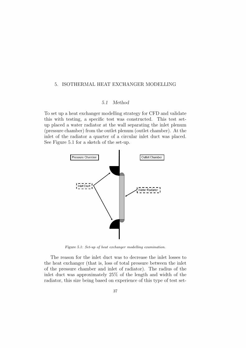
To set up a heat exchanger modelling strategy for CFD and validatethis with testing, a specific test was constructed. This test set-up placed a water radiator at the wall separating the inlet plenum(pressure chamber) from the outlet plenum (outlet chamber). At theinlet of the radiator a quarter of a circular inlet duct was placed.See Figure 5.1 for a sketch of the set-up.
Figure 5.1: Set-up of heat exchanger modelling examination.
The reason for the inlet duct was to decrease the inlet losses tothe heat exchanger (that is, loss of total pressure between the inletof the pressure chamber and inlet of radiator). The radius of theinlet duct was approximately 25% of the length and width of theradiator, this size being based on experience of this type of test set-
37

5. ISOTHERMAL HEAT EXCHANGER MODELLING
up. On the exit side no ducting of any sort was added. On thisside, the assumption of total loss of dynamic pressure on the exitwas made. This is according to the previous theory.
Firstly the assumptions of no inlet losses and full exit loss will bethoroughly investigated in this thesis. To explain the fluid dynamicsfurther, one must look into the complete flow of this test set-up. Toaid the discussion Figure 5.2 will be utilised.
Figure 5.2: Sketch showing the physics of the total pressure and losses for this testset-up and measurement procedure.
In a plenum to plenum test rig, such as the one utilised in thisthesis, the air flow rate through the rig together with the static pres-sure differential between the two plenums or chambers is measured.For this test condition, which aims to determine the heat exchangerpressure drop, correction of the plenum pressure drop measurementwith inlet and exit losses, so that it only contains the ”core only”pressure drop, is needed.
To explain the physics further: uniform flow enters the pressurechamber over a large area (making the velocity at the inlet lessthan 1m/s, hence the dynamic pressure is less than 1Pa). Since thedynamic pressure is so low, Equation (5.1) applies with the notationof Figure 5.2.
38
5.1. METHOD
pplenum,1 = pt,1 = ps,1 + pd,1︸︷︷︸
≈0
≈ ps,1 (5.1)
Then, due to the contraction ratio between the inlet wall andradiator, flow will accelerate down to the radiator, and static pres-sure will be converted to dynamic pressure (step 2 in Figure 5.2),furthermore since this is a plenum to plenum test facility inlet lossescan be present as well, in the form of loss of total pressure to tur-bulence (step 3 in Figure 5.2). These inlet losses are counter-actedby the inclusion of the inlet duct. At the inlet of the radiator, thefollowing pressure balance applies according to Equation (5.2).
pplenum,1 = ps,4,in + pd,4 + pinletloss,3 (5.2)
Through the radiator, static pressure will be lost due to the sur-face friction and turbulence in the core that is necessary for heattransfer. The pressure balance aft of the radiator at the point whereplenum outlet pressure is measured follows Equation (5.3).
pplenum,6 = ps,4,out + pd,4 + pexitloss,3 (5.3)
So, in this case, when one wants to measure the ”core only”pressure drop, Equation (5.4), by measuring the plenum pressure inthe two chambers, one needs to correct for dynamic acceleration,inlet and exit losses according to Equations (5.1 - 5.3).
∆pcore = ps,4,in − ps,4,out (5.4)
In this thesis three engineering approximations are made whenthe core only pressure drop is calculated from measurements. Firstly,the inlet duct is designed such that no inlet losses are present, sec-ondly, is that all of the dynamic pressure at the exit is lost, andthirdly, the dynamic pressure is calculated using the rig measuredvolumetric flow rate and the full core area according to Equation(5.5). These assumptions will be used and evaluated in the correla-tion study of heat exchanger pressure drop.
∆pd,4 =1
2ρ(
V
Acore
)2
(5.5)
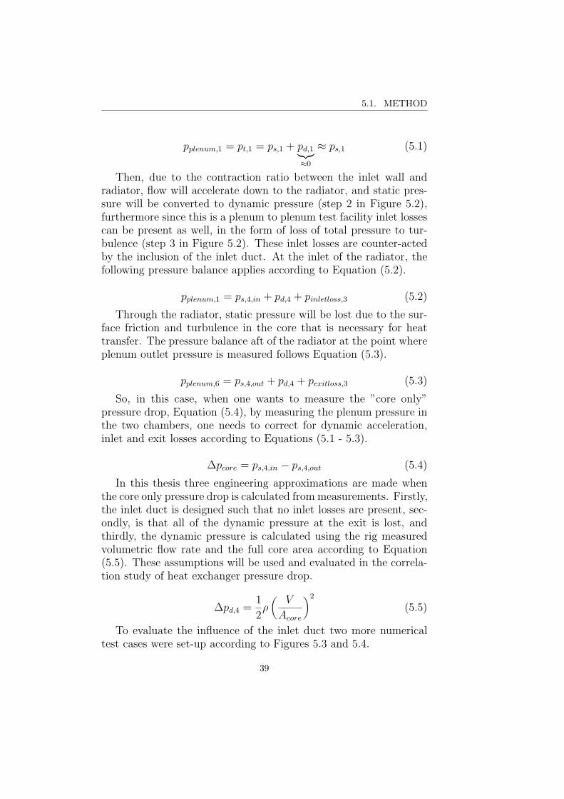
To evaluate the influence of the inlet duct two more numericaltest cases were set-up according to Figures 5.3 and 5.4.
39

5. ISOTHERMAL HEAT EXCHANGER MODELLING
Figure 5.3: Complimentary set-up of heat exchanger modelling examination.
5.1.1 Experimental Measurements
The experiments in this thesis were carried out in the Volvo 3P FanTest Rig, described in Section 2.1. For this part of the study a testwas set-up according to Figure 5.1. The static pressure was mea-sured between the two chambers as a function of different volumetricflow rates. All data is presented later for standard air conditions.The procedures to reach standardised outputs are described in Ap-pendix A.1 Standard Air Conditions.
5.1.2 Numerical Simulations
The computational part of this study utilised StarCCM+ version5.06.010. This software is developed and distributed by CD-adpacoand it is based on Navier-Stokes Equations, according to Section2.2.2.
For the test set-up a CAD model of the pressure chamber andoutlet chamber was created. The details of this can be seen in Figure5.5.
The basic principle of the numerical test rig was to incorporatea velocity inlet condition at the inlet face to the pressure chamber.
40
5.1. METHOD
Figure 5.4: Complimentary set-up of heat exchanger modelling examination.
By prescribing the inlet velocity, the volumetric flow rate was set.Furthermore the outlet chamber was maintained at ambient pressureby prescribing a pressure outlet boundary condition to the outletface of the test rig. For this part of the study incompressibility wasassumed, and by that, the density of air was set to standard aircondition. Finally the static pressure was measured between thetwo chambers in the same positions as for the actual test rig.
For the test set-up, three different models were built, each modelcorresponded to one of the Figures 5.1, 5.3 and 5.4. For the radiator,the supplier CAD data was used. The three different test cases aredescribed in Table 5.1.
From this CAD data, surface meshes were created in ANSA.These were later volume meshed in StarCCM+. The final volumemeshes consisted of 4.4 - 4.8 million cells with the main concen-tration around the heat exchanger, inlet duct and exit blast. Themeshes were pure Trim cell meshes (basically hexahedral cells). Theinlet duct was meshed with two layers of prism cells for this case.Figure 5.6 shows the section geometry of essential parts for this testset-up. This figure illustrates the cell density distribution locallyaround the test object.
41

5. ISOTHERMAL HEAT EXCHANGER MODELLING
Figure 5.5: A side view of the resulting 3D CAD Model of the Volvo 3P Fan Test Rig.Shaded in green is the pressure chamber, in light brown the outlet chamber.
Name Description FigureBaseline Baseline model with 5.1
inlet ductNo duct Radiator placed in 5.3
outlet chamber withno duct
No duct p Radiator placed in 5.4pressure chamber withno duct
Table 5.1: Numerical test cases for heat exchanger modelling.
Furthermore in StarCCM+ the cases were set up and solved for.The main settings in the CFD solver for all of the three cases wereas follows:
• This study used 3D incompressible Reynolds Averaged Navier-Stokes equations.
• The segregated solver together with second order discretisationschemes were used.
• The air density was set to standard air conditions (1.2kg/m3).
• Turbulence was modelled using Realizable k-epsilon, two layermodel (shear driven, Wolfstein).
• Walls were modelled using two layer all y+ wall treatment. y+spanned at the majority of surface cells between 30-100.
• Boundary conditions were velocity inlet and pressure outletpositioned to the right and left respectively in Figure 5.5.
42

5.2. RESULTS AND DISCUSSION
Figure 5.6: Section geometry visualising the mesh density of the radiator modellingmesh.
• The core of the heat exchanger was modelled using the assump-tion of porous media, described in Section 2.2.2 Porous Media.
Based on the assumption of no inlet losses and total exit losses,the heat exchanger pressure drop coefficients of Equation 2.8 werederived from the experimental test results. In this manner by com-paring the predicted plenum pressure loss with that measured, thedynamic pressure corrections could be validated. Moreover, theCFD data could be used for understanding the physics in more de-tail.
For the second and third test cases of Table 5.1, the same coeffi-cients in the radiator were used as derived for the first test case.
5.2 Results and Discussion
The first step in this examination was to measure the plenum pres-sure drop of the heat exchanger in a test set-up according to Figure5.1. This was partly to calibrate the porous coefficients for the CFDmodel, and also to serve as the tested data to correlate the simula-tions of this test set-up. The plenum pressure drop of the measured
43

5. ISOTHERMAL HEAT EXCHANGER MODELLING
test set-up is presented in Figure 5.7. Together with the test data, asecond order polynomial is fitted to this data according to Equation(2.8). Visible in this figure is a clear indication that the division ofa viscous and inertial term for the heat exchanger core is a logicalassumption. This is demonstrated by the fact that a second orderpolynomial fits the measured data well.
Figure 5.7: Plenum pressure drop data of the heat exchanger. TD = Tested Data.
After this, the assumption regarding inlet and exit losses wasmade to the data of Figure 5.7. Note that a correction of dynamicpressure due to inlet and exit losses is an inertial correction. Thusthe correction only changes the second order term of the polyno-mial fit in Figure 5.7. With this assumption the porous resistancecoefficient was derived using the polynomial data in Figure 5.7 andEquation (2.8). With this data entered into the CFD model accord-ing to Figure 5.6, simulations of the calibration process were madeto observe the results of the assumption regarding inlet and exitlosses. The results presented together with the measurements aregiven in Figure 5.8.
Figure 5.8 displays a very good match of the simulated plenumpressure to the test data. This confirm that the used test proce-dure and correction method works for the task of deriving porousresistance coefficients for the radiator and test set-up.
Of more interest is the fact that the simulated calibration can beused to extract the static pressure losses associated with the inletand exit of the test condition according to Figure 5.1, and also as
44
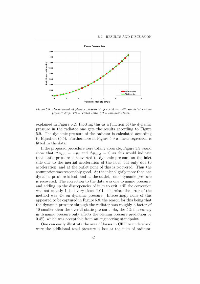
5.2. RESULTS AND DISCUSSION
Figure 5.8: Measurement of plenum pressure drop correlated with simulated plenumpressure drop. TD = Tested Data, SD = Simulated Data.
explained in Figure 5.2. Plotting this as a function of the dynamicpressure in the radiator one gets the results according to Figure5.9. The dynamic pressure of the radiator is calculated accordingto Equation (5.5). Furthermore in Figure 5.9 a linear regression isfitted to the data.
If the proposed procedure were totally accurate, Figure 5.9 wouldshow that ∆ps,in = −pd and ∆ps,out = 0 as this would indicatethat static pressure is converted to dynamic pressure on the inletside due to the inertial acceleration of the flow, but only due toacceleration, and at the outlet none of this is recovered. Thus theassumption was reasonably good. At the inlet slightly more than onedynamic pressure is lost, and at the outlet, some dynamic pressureis recovered. The correction to the data was one dynamic pressure,and adding up the discrepencies of inlet to exit, still the correctionwas not exactly 1, but very close, 1.04. Therefore the error of themethod was 4% on dynamic pressure. Interestingly none of thisappeared to be captured in Figure 5.8, the reason for this being thatthe dynamic pressure through the radiator was roughly a factor of10 smaller than the overall static pressure. So, the 4% inaccuracyin dynamic pressure only affects the plenum pressure prediction by0.4%, which was acceptable from an engineering standpoint.
One can easily illustrate the area of losses in CFD to understandwere the additional total pressure is lost at the inlet of radiator;
45

5. ISOTHERMAL HEAT EXCHANGER MODELLING
Figure 5.9: Static inlet and exit pressure losses plotted as a function of dynamic pres-sure through the core of the radiator.
by plotting the iso-surface of total pressure = predicted plenumpressure, see Figure 5.10. Shown in this figure are zones that havelower total pressure than the plenum pressure, hence it is here thelosses that are not covered by Bernoulli are shown. In this figureis the corresponding boundary layer growth on the inlet duct itself,and a vortex structure on the vertical centre-line of the radiator.
One could correct the method by accounting for the effects ofboundary layer, hence increasing the calculated dynamic pressure.Note that the measured acceleration loss is plotted against the dy-namic pressure of the flow rate spread over the entire area of theradiator. With the effects of boundary layer, a small contractionoccurs, so in reality the dynamic pressure through the radiator ishigher than calculated.
With regards to the two vortices seen in Figure 5.10, these occuras a result of the geometrical configuration of the test chamber andare secondary flow effects. These are definitely more difficult tocorrect for.
At the exit side of the heat exchanger, Figure 5.9 indicates asmall recovery of dynamic pressure. This was what occured andsummarising the two; inlet and exit effects, one roughly lose a factorof 1.04 dynamic pressure for this type of test set-up.
The results for the remaining two numerical test set-ups withoutthe inlet ducting, are shown in Figures 5.11 and 5.12. It will be
46

5.2. RESULTS AND DISCUSSION
Figure 5.10: Iso-surface of total pressure = inlet pressure for flow rate 6m3/s.
seen that, without the inlet duct, approximately 20% more staticpresssure is lost at the inlet; and furthermore by placing the radiatorin the pressure chamber, in the region of 40% more static pressureis lost.
Figure 5.12 shows the effect these test conditions had on thepredicted plenum pressure. It can be seen that, if the inlet ductwould have been excluded, the correction method applied wouldnot have been valid.
This part of the study correlated quite well to classical literature.This is the typical behaviour of flow that makes sudden expansionsor contractions. White, [3], amongst others, has documented thesephenomena rather well, see chapter 6.9. Minor Losses in Pipe Sys-tems. In this chapter White introduced a loss factor, K which wasthe static pressure loss normalised by the dynamic pressure goingthrough the smallest diameter pipe (the dynamic pressure throughthe radiator, in this thesis). For a sudden expansion this followsEquation (5.6) and for a sudden contraction this follows Equation(5.7). d being the smaller diameter and D the larger diameter.
47

5. ISOTHERMAL HEAT EXCHANGER MODELLING
Figure 5.11: Static inlet and exit pressure losses plotted as a function of dynamic pres-sure through the core of the radiator.
KSE =
(
1− d2
D2
)2
(5.6)
KSC ≈ 0.42
(
1− d2
D2
)
(5.7)
For the Volvo test rig, the hydraulic diameter of the radiatormust be calculated, as well as the inlet and exit area of the test rig.Inserting this data into the above equations resulted in a recoveryof 6% of the dynamic pressure at the exit and in addition an inletloss of 40% dynamic pressure.
As a final comment, the losses at the exit correlated rather well,however at the inlet it was more difficult, and it is probable thatthe proposed correction by White cannot be used here, due to theinclusion of the radiator, and the fact that this causes a severe pres-sure gradient upstream of the radiator; and this was not present inWhite’s contraction correction. Even so, the correct physics phe-nomena was explained by this method.
5.3 Intermediate Summary and Conclusions
This chapter has examined how to measure the porous resistancecoefficients for CFD simulations, using a plenum to plenum test rig.
48

5.3. INTERMEDIATE SUMMARY AND CONCLUSIONS
Figure 5.12: Measurement of plenum pressure drop correlated with simulated plenumpressure drop. TD = Tested Data, SD = Simulated Data.
The methods used in this chapter resulted in an accuracy of 0.4%.Special care needs to be taken with the inlet side of the radiator,
and the inlet must be controlled for the assumptions made to bevalid.
49

5. ISOTHERMAL HEAT EXCHANGER MODELLING
50

6. FAN MODELLING
6.1 Method
To set up a fan modelling strategy in CFD and validate this strategywith test data, a specific test set-up was constructed. This test set-up positioned a production fan inside a production fan ring, and theoutlet of the fan ring was aligned with the wall separating the inletplenum to the outlet plenum of the test rig. In front of the fan ringa production square fan shroud was placed, and after the fan a 3Dengine silhouette was placed. See Figure 6.1 for a sketch of the testset-up.
Figure 6.1: Set-up of fan modelling components.
The fan ring and fan shroud were connected by a rubber seal.This was due to the fact that: in a truck, the fan ring is enginemounted and the shroud is chassis mounted, so a flexible seal is
51

6. FAN MODELLING
required to allow relative movements.The reasoning behind this test set-up was: this is how a truck
fan is installed in most current premium trucks. This motivates thesemi-complex test set-up. Standardised fan tests on the other handtypically only test the fan, and not necessarily the fan installed in afan ring. It is common to test fans installed into a flat plate orifice(FPO). Meaning the fan simply placed in a circular hole in the wall.The tip clearance for these type of tests typically range from 12.5mm(0.5”) to 25mm (1”).
Since FPO testing is a poor representation of a typical coolingfan installation, such as presented by Wang et.al. in [20], this testmethod was discarded. Instead a more realistic set-up was chosen,complying to the above specification. Comparing with the FPOstandard, this test included a tight tip clearance fan ring. Tipclearance in the test was 6mm compared to 12.5mm or 25mm, thusprohibiting over-flow at the fan blade tip. Finally this test also in-corporated the first parts in front of, and after the fan that is notrotationally symmetrical, since in a typical installation these arepresent and interact with the fan.
Of course it can be argued that this test is still too simplistic,since it did not incorporate the heat exchangers and parts in frontof these and the full installation behind the fan. But with this testset-up it was possible to control the test objects precisely, both inCAD and physical testing.
For this set-up, production parts were used for the fan, shroud,ring and seal. For the engine mock-up a 3D SLA silhouette was used.For the simulation, the corresponding CAD data of the productionparts was used. For the 3D silhouette, the actual STL model thatwas used to manufacture the SLA model was used as a representa-tion of the same part.
For this thesis the focus was not only on predicting one fan,but several. Table 6.1 details the four fans that were examined indifferent aspects of fan modelling techniques for this thesis.
A short description of the fans is given below. For the productionfans, these were typically made of polyamid reinforced with 20-30%glass-fibre.
Fan:
I This can be considered the classical axial production fan with 8blades. The blades are what one would consider heavily loaded.
52

6.1. METHOD
Fan Type Diameter Blade # DesignFan I 750mm 8 ClassicFan II 750mm 11 ModernFan III 750mm 11 ExperimentalFan IV 680mm 8 Classic
Table 6.1: Tabulated series of fans.
Meaning, that in a truck installation they operate at quite ahigh angle of attack. This also means that the blades are oper-ated close to stall.
II In comparison to (I), this fan was a moden production fan. Ithad 11 blades. It was considered modern for a number of rea-sons. First of all this fan had a large hub area. This was notfor aerodynamic performance, this was to be able to fit a largerviscous clutch. A large viscous clutch is required to be able tocontrol the fan correctly, whilst still high power is fed into thefan. With a large hub there is less space for fan blades, so toget competitive performance of the blades compared to olderfans, these blades are operated closer to stall. Furthermore thisfan had flow stabilising devices at the root of the blade, typ-cially these are placed there to control the fan stall in a stableway. These stabilising devices are typical for modern fans. Fur-thermore they can sometimes aid the clutch, by increasing thecooling of the clutch.
Finally this fan having 11 blades typically allows it to operatewith higher throttling, or angle of attack.
III This fan was an experimental fan. It had 11 blades whichwere medium loaded. It was made out of aluminium and moreuniquely this fan had a diagonal hub, diagonal blades and adiagonal fan ring.
IV This fan was of the same design as the first fan, with the excep-tion that the blades of this fan were cut from 750mm to 680mm.This means that it is a ”production” scaling done to this fan,and not an aerodynamical scaling.
For the default test set-up the test fans and components werepositioned relative to each other at a set distance. The distance
53

6. FAN MODELLING
between fan ring and fan shroud was 15mm axially. The distancebetween the trailing tip of the fan blade and the most rearward faceof the fan ring was 25mm. And the clearance between the trailingtip of the fan blade to the forward face of the engine mock-up was20mm. This setting was used for all of the correlation cases.
6.1.1 Experimental Measurements
The experimental part of this study was carried out in the Volvo3P Fan Test Rig, described in Section 2.1. And for this part ofthe study a test was set up according to Figure 6.1 with the fourdifferent fans according to the description above.
For these experiments the static pressure differential was mea-sured between the two chambers as a function of different volumetricflow rates. This was done for fixed fan speeds. The fan performancewas measured for two speeds, the default speed of 40rps, and at20rps. The lower speed was measured so that the fan laws thatwere described in Section 2.2.1 Fan Laws could be used to checkthat the default test was carried out without the influence of struc-tural deformations.
It should be remembered that the fan laws are derived assuminginertial flow and structural rigidity, that is, that the blades do notalter shape during testing, while fan speed and fan load varies. Thelatter statement holds the key to a very beneficial feature of the fanlaws for this study. If the fan is tested for two speeds, the correlationspeed and one speed which is significantly lower, the fan laws canbe applied to the lower speed, to correct these measurements forthe chosen correlation speed. If the fan laws are shown to applythey can be used to prove the following two facts: One, the flow isinertial (though it is better to prove this by calculating the Reynoldsnumber for the problem), and two; the test object is not subjectedto deflections during testing.
If the fan laws do not apply, one can point to the fan law assump-tion of rigidity and assume that the fan is not rigid during testingfor the higher fan speed. Hence, the simulated geometry and thetested geometry are no longer identical.
From the speed viewpoint, note that the load on the blade in-creases by the square of rotational speed, both for pressure load,Equation (2.3), and centripetal load (classical mechanics). This cri-
54

6.1. METHOD
teria can be used to check for structural deformations in testing.To summarise; by measuring fan performance data at two differentspeeds the fan laws can be used for checking the test for structuraldeformations.
During fan performance testing, fan power consumption was alsomeasured. The details of this is presented in Appendix A.1 Measur-ing Fan Power.
All data is presented for standard air conditions later. The pro-cedure to achieve standardised outputs are described in AppendixA.1 Standard Air Conditions.
Finally a separate test was set up. This has not been used tocorrelate experiments with simulations. What separated this testfrom the default testing was that the fan was positioned differently.Instead of having a fan protruding 25mm out of the fan ring, it onlyprotruded 15mm. Furthermore the spacing between the fan andmock-up was 15mm, not 20mm as for the default test. This testwas designed to examine fan modelling strategies for more severeinstallation conditions, but up to the time of writing, the simulationsfor this had not been carried out. However, of interest is that forthe second fan, Fan II, this test was repeated four times duringthis project. And this gives an insight to the testing capability andrepeatability of the experiments.
Table 6.2 summarises all the fan tests that were carried out:
Fan Type Speed Test Type CommentFan I 20rps Default Test N/AFan I 40rps Default Test N/AFan II 20rps Default Test N/AFan II 40rps Default Test N/AFan III 20rps Default Test N/AFan III 40rps Default Test N/AFan IV 20rps Default Test N/AFan IV 40rps Default Test N/AFan II 40rps 2nd Test Set-up 2009-04Fan II 40rps 2nd Test Set-up 2009-12Fan II 40rps 2nd Test Set-up 2010-04Fan II 40rps 2nd Test Set-up 2010-06
Table 6.2: Tabulated series of fan tests.
55

6. FAN MODELLING
6.1.2 Numerical Simulations
The main focus of this thesis and research project has been howcooling airflow in CFD can be modelled, what capabilities there wereavailable and what level of computational effort these required.
Regarding fan modelling strategies in CFD, the main focus hasbeen on the fan MRF model and fan sliding mesh model. The rea-sons for this was that both of these models do not rely on any pre-viously tested performance data. What separates them is accuracycomparred to computational effort.
The first piece of work that was published in this research projectwas a paper comparing the MRF model to sliding mesh for a sys-tem, not just incorporating the fan but also radiator and a shroudcovering the outlet of the fan. That paper used the CFD softwareStarCD and StarCCM+. Both developed and distributed by CD-Adapco. This was Paper I and what was found in that paper wasthat the sliding mesh model, in principle, had good capabilities forfan modelling whereas MRF under-predicted fan performance sig-nificantly.
With that work as a background, a study was initiated to examinethe detailed performances of the two different fan models and mapout model capabilities in predicting performance as a function ofcomputational effort.
Surface Data
For the numerical test set-up the same CAD model of the pressurechamber and outlet chamber as in the previous chapter and Figure5.5, was used. For the test components according to Figure 6.1,CAD data were used. Additionally for this part of the study a CADmodel of the motor that drives the fan and measures fan powerconsumption was included.
For the fan ring and shroud, these were designed in-house atVolvo, so these components have been checked to ensure that theactual parts produced correlate to the intended design. For the 3Dengine silhoutte, the surface STL data that was used to make thatprototype, was used in the surface model as well.
Finally, the fans; for Fan I, supplier CAD data was used. Theinitial CAD data was found to be erroneous, so that an update wasmade to this data once this was discovered. This fan was of such an
56

6.1. METHOD
age that it almost pre-dated 3D CAD, and the initial CAD data wasout-dated. For Fan II, this fan was sent for laser scanning, and thusit was possible to confirm that the actual CAD data correspondedwell to the actual test piece. For Fan III this was an aluminiummilled experimental fan, and the same CAD data was used for sim-ulations, as was used for the machining. In this case any error of thefan geometry would have been due to the capabilities of reproducingthe CAD data by the CNC milling machine. For the Fan IV, similarcomments apply as for Fan I.
For each model, the CAD data was entered into ANSA, a pre-processing tool developed by BETA CAE Systems. In ANSA a sur-face mesh was created for all of the simulations. Since this projectspanned a number of years, several versions of ANSA have beenused, ranging from the earliest releases of version 12 to the latestreleases of version 13.
RANS Investigations
For numerical RANS simulations, StarCCM+ was used. The ver-sions have been ranging from StarCCM+ version 2, to version 6.The main settings in the CFD solver were as follows:
• This study used 3D incompressible Reynolds Averaged Navier-Stokes equations.
• The segregated solver together with second order discretisationschemes were used.
• The air density was set to standard air conditions (1.2kg/m3).
• Turbulence was modelled using Realizable k-epsilon, two layermodel (shear driven, Wolfstein).
• Walls were modelled using two layer all y+ wall treatment. y+spanned at the majority of surface cells between 30-100.
• Boundary conditions were velocity inlet and pressure outletpositioned to the right and left respectively in Figure 5.5.
The meshing strategy, for all investigated cases, was to have amain concentration of cells around the fan, shroud and engine mock-up. The fan region was as per default meshed using polyhedral cellsand the rest were meshed using Trim cells (basically hexahedral
57

6. FAN MODELLING
cells). Objects that are of significant aerodynamic importance weremeshed with two layers of prism cells. Table 6.3 outlines the defaultconstraints.
Region Mesh Type Minimum Size Maximum SizeFan Domain Poly + Prism 0.5mm 8mmRefinement 1 Trim + Prism 1mm 8mmRefinement 2 Trim + Prism 1mm 40mmPlenum Domains Trim 10mm 250mm
Table 6.3: Mesh Constraints.
In total the cases comprised 8-18 million cells. The count de-pended on the size of MRF domain and blade count. The larger thedomain and more blades, the more cells were required with respectto Table 6.3.
Polyhedral cells in the fan region was used because, typically,there is high numerical diffusion associated with CFD when theflow is not aligned with, or perpendicular to, the cell faces. Thepolyhedral cell more frequently has one face that is orientated per-pendicular to the local flow, since it has far more faces than hexahe-dral or tetrahedral cells. Since this study will span several differentworking regions of the fan, highly complex and non-aligned flow willbe simulated and this motivates the use of polyhedral cells.
As for the inlet and outlet domain, hexahedral cells were used tokeep the cell and face count, and also the run time, to a reasonablelevel. These regions still contain complex flows, but not of the sameorder of magnitude as the fan domain.
Domain influenceAt the start of the investigations of the MRF model and its ca-
pabilities, it was stated in the the chapter of Theory that the MRFmodel relies on a previously defined rotational volume or domain.It was also found by Wang et.al in [20] that the choice of domainstrongly affected the predicted fan performance. Following this, anumerical test was set up that investigated four different rotationaldomains. These are shown in Figure 6.2. In Figure 6.2 the pressurechamber can be seen to the left, and outlet chamber together withthe engine mock-up and motor that drives the fan to the right. Thedetails of the figure and its corresponding domains are explained in
58

6.1. METHOD
Table 6.4.
Figure 6.2: The four different MRF domains.
For this investigation Fan I was investigated for all of the do-mains. Fan II only for domain I and III. Fan III only for domainIII and Fan IV only for domain I. Figure 6.3 illustrates the typicalmesh resolution for the cases. This figure shows Fan I for domainIII. Table 6.5 lists all of the prestented simulations.
As will be shown, the strong influence of the MRF domain onpredicted fan performance will be replicated. For the cases that didnot reproduce the measured fan performance it was of interest tomeasure the error of prediction. So, for this purpose, a standardisedmethod of measuring the error, that was logical from the coolingairflow perspective, was required. It was also interesting to use thisstandard and compare the consistency of the fan MRF model acrossfans of different designs.
For these reasons Fan I was simulated for domain I at not just thedefault fan speed of 40rps, but also 20rps. By applying the fan laws,Section 2.2.1 Fan Laws, to the 20rps data and re-scaling it to 40rps,
59

6. FAN MODELLING
Domain Colour DescriptionI Yellow Circular domain, domain divides blade tip clearance
in half. Rear face splits the distance between fanand engine mock-up in half. The forward face spansapproximately the same distance forward.
II Yellow This domain is grown out to the fan ring andRed incorporates this counter-rotating in the
rotating coordinate system.III Yellow This domain extends rearward to the forward
Red face of engine mock-up and extendsGreen forward to meet the forward face of shroud.
Furthermore the rearward face is extended 15mmradially at the exit.
IV Yellow This domain is expanded forward to span half theRed pressure chamber and extended rearward as far asGreen possible before interferring with non-rotationallyOrange symmetric parts.
Table 6.4: Details of the different fan domains according to Figure 6.2.
it was possible to check whether the error caused by MRF scaledwith inertial scaling laws or not. Table 6.6 tabulates the extendedstudy of domains and fan speeds.
To measure the error caused by the MRF model, the fan lawswere used once more. By taking the erroneously predicted data,applying the fan laws, and rescaling the simulated data with a fanspeed ratio, to get the measured and re-scaled data to line up, therescaling factor effectively becomes a measurement of the error. Inthe context of cooling airflow and fan airflow, the volumetric flowrate is linear with fan speed, see Equation (2.2), so that the rescalingfactor effectively becomes the error of fan flow rate prediction. Thiswill also hold true in a system if the system pressure drop is scaledpurely according to inertial scaling laws, like Equation (2.3). This isnot exactly the case for a truck cooling system, as there are viscouseffects, that is for the heat exchanger and this can be describedwith a linear term and a quadratic, see Equation (2.8). But based onexperience, the stronger of the two influences are the quadratic term.So that this measure of error can be extrapolated to a measurementof error of flow rate in the cooling airflow system.
Typically, representing the pressure drop curve with an exponen-tial function instead of a polynomial, a system exponential of 1.6 to
60
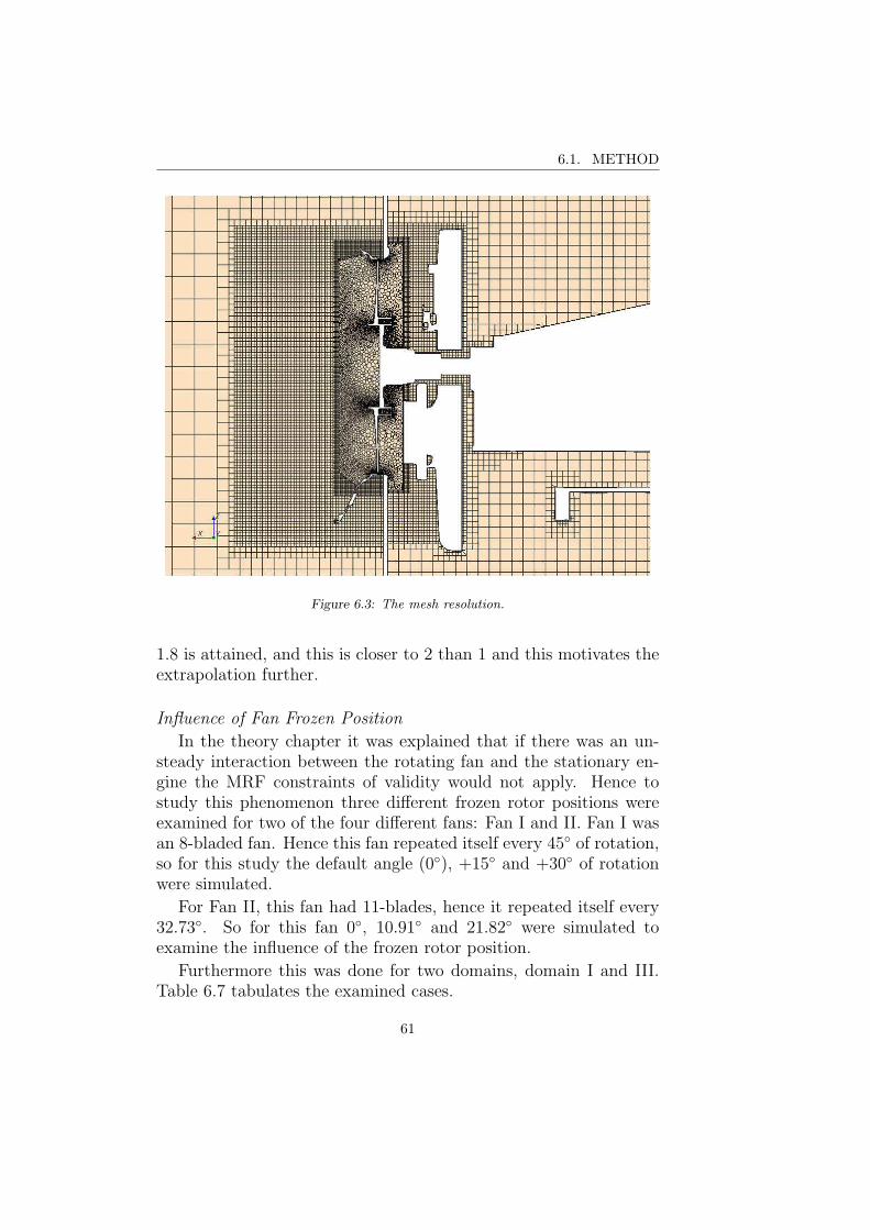
6.1. METHOD
Figure 6.3: The mesh resolution.
1.8 is attained, and this is closer to 2 than 1 and this motivates theextrapolation further.
Influence of Fan Frozen Position
In the theory chapter it was explained that if there was an un-steady interaction between the rotating fan and the stationary en-gine the MRF constraints of validity would not apply. Hence tostudy this phenomenon three different frozen rotor positions wereexamined for two of the four different fans: Fan I and II. Fan I wasan 8-bladed fan. Hence this fan repeated itself every 45◦ of rotation,so for this study the default angle (0◦), +15◦ and +30◦ of rotationwere simulated.
For Fan II, this fan had 11-blades, hence it repeated itself every32.73◦. So for this fan 0◦, 10.91◦ and 21.82◦ were simulated toexamine the influence of the frozen rotor position.
Furthermore this was done for two domains, domain I and III.Table 6.7 tabulates the examined cases.
61

6. FAN MODELLING
Fan DomainFan I Domain IFan I Domain IIFan I Domain IIIFan I Domain IVFan II Domain IFan II Domain IIIFan III Domain IIIFan IV Domain I
Table 6.5: Tabulated series of cases for domain study.
Fan Domain SpeedFan I Domain I 20rpsFan I Domain I 40rps
Table 6.6: Tabulated series of cases for extended domain study.
Influence of Turbulence Models and Computational Grid
In a commercial CFD solver based on RANS typically a set ofmodels are available to choose between for various topics of numericsand physics. These range from discretisation schemes of the RANSequations presented in Appendix A.2, to the turbulence models andhow one distributes the cells in the domain.
Among the settings for a typical RANS simulation, and how thesechoices of settings influence the simulated results, it is typical to lookinto the influence of user specific choice of turbulence model and howgrid independent the results are.
As previously stated the default turbulence model for this part ofthe thesis was Realizable k-epsilon. Additionally two other modelswere examined; k-omega SST and Quadratic k-epsilon. These arepresented in further detail in Appendix A.2.
This examination focused on Fan I, domain III and the defaultblade position angle.
For Fan I, domain III and the default blade position angle, aminor mesh study was conducted. This was done for two flow ratepoints, 11.6 m3/s and 7.44 m3/s. Table 6.8 outlines the details of theexamined cases. For comparison, the results from the examinationof frozen position of the fan for the default mesh, will be presentedtogether with this examination.
62
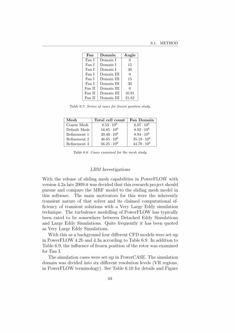
6.1. METHOD
Fan Domain AngleFan I Domain I 0Fan I Domain I 15Fan I Domain I 30Fan I Domain III 0Fan I Domain III 15Fan I Domain III 30Fan II Domain III 0Fan II Domain III 10.91Fan II Domain III 21.82
Table 6.7: Series of cases for frozen position study.
Mesh Total cell count Fan DomainCoarse Mesh 8.53 · 106 6.07 · 106Default Mesh 16.85 · 106 8.92 · 106Refinement 1 20.40 · 106 8.94 · 106Refinement 2 46.65 · 106 35.19 · 106Refinement 3 56.25 · 106 44.78 · 106
Table 6.8: Cases examined for the mesh study.
LBM Investigations
With the release of sliding mesh capabilities in PowerFLOW withversion 4.2a late 2009 it was decided that this research project shouldpursue and compare the MRF model to the sliding mesh model inthis software. The main motivators for this were the inherentlytransient nature of that solver and its claimed computational ef-ficiency of transient solutions with a Very Large Eddy simulationtechnique. The turbulence modelling of PowerFLOW has typicallybeen rated to be somewhere between Detached Eddy Simulationsand Large Eddy Simulations. Quite frequently it has been quotedas Very Large Eddy Simulations.
With this as a background four different CFD models were set-upin PowerFLOW 4.2b and 4.3a according to Table 6.9. In addition toTable 6.9, the influence of frozen position of the rotor was examinedfor Fan I.
The simulation cases were set-up in PowerCASE. The simulationdomain was divided into six different resolution levels (VR regions,in PowerFLOW terminology). See Table 6.10 for details and Figure
63

6. FAN MODELLING
Fan Fan ModelFan I MRFFan I SMFan II SMFan III SM
Table 6.9: Cases examined in PowerFLOW.
6.4 which highlights the 5 largest domains. The bounding surfaceof the Fan Test Rig constituted the first level of resolution. And insteps of two, the resolution was increased around the test object andtest set-up. This can be clearly seen in Figure 6.4, and highlightedby three orange Cartesian boxes. The fourth domain of furtherincreased resolution was the LRF domain which is an offset fromthe cylindrical LRF region. This is shown in figure 5 by the redbox. LRF domain is PowerFLOW terminology, more details of thiscan be found in Appendix A.2 Local Reference Frames (LRF). Thefinal domain, domain 5 was a further increase of resolution aroundthe fan blades. This was made by a surface offset of the fan blades.
Resolution DescriptionLevel 1 0.040 m/voxel Bounding simulation domainLevel 2 0.020 m/voxel VR1 CartesianLevel 3 0.010 m/voxel VR2 CartesianLevel 4 5.00e-03 m/voxel VR3 CartesianLevel 5 2.50e-03 m/voxel VR4 LRF DomainLevel 6 1.25e-03 m/voxel VR5 Fan blade offset
Table 6.10: Mesh resolution. Voxel is PowerFLOW terminology for volume element.
As mentioned previously, both the MRF and SM technique reliedon a user-defined rotational volume. The two domains used in thisstudy are presented in Figure 6.5. It should be noted that the MRFdomain was significantly larger than the SM domain and that theMRF region corresponded well to domain III of previous section.Theoretically it was expected that the results of SM simulationsshould be less sensitive to the domain size, as long as all rotatingcomponents were completely enclosed by the LRF domain.
This set-up gave a total volume element (voxels, in PowerFLOWterminology) count of 28 million for the SM case and 29 million forthe MRF case, since the LRF domain was slightly larger for the
64

6.2. RESULTS AND DISCUSSION
Figure 6.4: Side view of the test set-up with the different mesh resolution regions high-lighted.
MRF case.The time step for these simulations was 2 microseconds and cases
typically converged after 500,000 time steps. For the case set-up Exabest practices were followed.
6.2 Results and Discussion
6.2.1 Experimental Measurements
The first part of this study was to measure the fan pump perfor-mance and fan power consumption for the four different fans in Table6.1 according to the specifications of Table 6.2. This was done partlyto get test data to correlate later simulations to, and also to use thefan laws to check the rigidity of the test components. The last setof tests were done to document the repeatability of the test rig andtest procedure.
The tests were carried out according to the description in thesection of Method and the set-up followed Figure 6.1.
For the four different fans, the result in Figures 6.6 - 6.9 wereachieved. Furthermore the repeatability result can be seen in Figure6.10
Looking at Figure 6.6 what can be seen is three different fanpump curves (static pressure rise of the fan for a fix rotation speed)and their corresponding fan power curves. In this figure is the per-formance data of Fan I, measured at 20 and 40rps, and also the20rps data re-scaled using the fan laws to 40rps. In this figure it
65
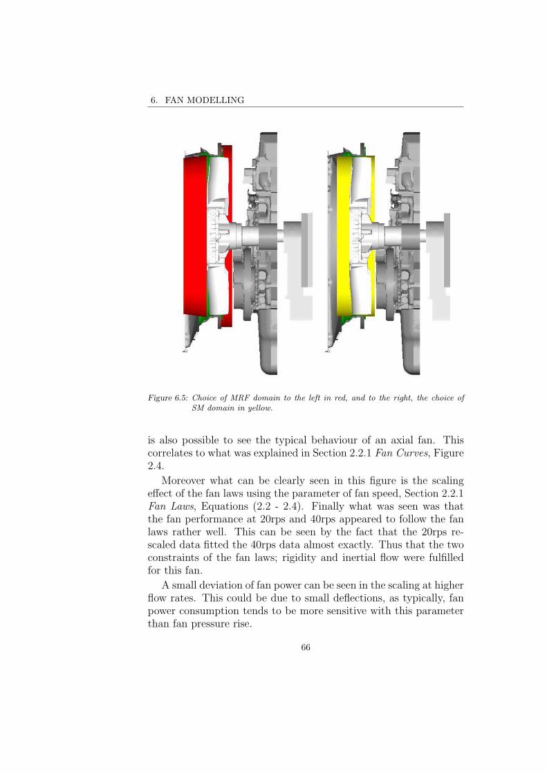
6. FAN MODELLING
Figure 6.5: Choice of MRF domain to the left in red, and to the right, the choice ofSM domain in yellow.
is also possible to see the typical behaviour of an axial fan. Thiscorrelates to what was explained in Section 2.2.1 Fan Curves, Figure2.4.
Moreover what can be clearly seen in this figure is the scalingeffect of the fan laws using the parameter of fan speed, Section 2.2.1Fan Laws, Equations (2.2 - 2.4). Finally what was seen was thatthe fan performance at 20rps and 40rps appeared to follow the fanlaws rather well. This can be seen by the fact that the 20rps re-scaled data fitted the 40rps data almost exactly. Thus that the twoconstraints of the fan laws; rigidity and inertial flow were fulfilledfor this fan.
A small deviation of fan power can be seen in the scaling at higherflow rates. This could be due to small deflections, as typically, fanpower consumption tends to be more sensitive with this parameterthan fan pressure rise.
66

6.2. RESULTS AND DISCUSSION
Figure 6.6: Measured fan pump performance and power consumption for Fan I, 40rps,20rps and 20rps re-scaled with the fan laws. TD = Tested Data.
From the above, the experimental results of Fan I, Figure 6.6, toFan II, Figure 6.7 could be compared. It was then seen that thefan laws did not apply completely, either for the pressure or powercurves. Since the Reynolds number was roughly the same, and thefan speeds were very high, the constraint of inertial flow shouldhave been fulfilled, indicating that this fan was deforming. Withthis conclusion, and taking into account the fact that the pressurerise over the blade and also that the centrifugal load increases bythe square of fan speed, the re-scaled 20rps data was the data thatmore closely resembled the un-deformed fan blades fan performance.That is, a rigid fan would produce results close to this performance.Consequently, for the later purposes of this study, this re-scaled datashould be used to compare simulations to, since the simulations werecarried out under the assumption of fan rigidity.
Moving on to the third fan, Figure 6.8, in this figure two thingscan be seen, first, that this aluminium fan was rigid, the fan lawsapplied very well. But of more interest was a clear scatter of mea-surement points at the fan transition point, the knee in the curve. Itshould be noted here that, for all of the measurements presented inFigures 6.6 - 6.10, each flow rate point actually represents 10 discretesamples. This cannot be clearly seen in Figures 6.6 and 6.7, sincethese fans had very stable operation at each of the sampled points.
67

6. FAN MODELLING
Figure 6.7: Measured fan pump performance and power consumption for Fan II, 40rps,20rps and 20rps re-scaled with the fan laws. TD = Tested Data.
However for the rigid experimental fan, Figure 6.8, instability canbe clearly seen for the transition point.
For the fourth fan, similar behaviour as the second fan was seen.The rigid assumption did not seem to apply completely. In this case,since this fan should have corresponded more to the first fan withregard to rigidity, it was actually discovered, that the wall separatingthe different plenums, and which the fan ring was attached to, wasdeforming due to the load. It should be pointed out that the 680mmand 750mm fans use different walls. And the 680mm wall was foundto be not as rigid as the 750mm. This test should of course havebeen repeated with a better wall, but the test was only used for onesmall correlation, and for its purposes, the data was good enough.
Finally, the repeatability of the test rig was examined, Figure6.10. In this figure the same fan, Fan II, was tested four timesover a 14 months period. Measurements were carried out duringspring, summer and winter, thus covering a wide range of ambientconditions regarding barometric pressure and humidity.
The following can be seen in the figure:
1. The ambient corrections applied to the test data, presented inAppendix A.1, appeared to function for this range of opera-tions.
68

6.2. RESULTS AND DISCUSSION
Figure 6.8: Measured fan pump performance and power consumption for Fan III,40rps, 20rps and 20rps re-scaled with the fan laws. TD = Tested Data.
2. The test procedure and test facility was controllable and re-peatable. Figure 6.10 illustrates that the test could be repeatedaccurately multiple times.
In this context it should also be mentioned that the test rig wascalibrated regularly, different types of calibrations were carried outat different intervals. Every six months the pressure sensors werecalibrated and the electronic signal system was controlled. In similarmanner the rig was checked for leakages and temperature sensorswere calibrated. Every three years the complete volumetric flowrate measurement facility is checked with a calibrated nozzle.
With the evidence of Figure 6.10, the maintenance protocol ap-peared to be correct.
69

6. FAN MODELLING
Figure 6.9: Measured fan pump performance and power consumption for Fan IV,40rps, 20rps and 20rps re-scaled with the fan laws. TD = Tested Data.
6.2.2 Numerical Simulations
RANS Investigations
For the RANS part of the investigation the follwing results wereobtained.
Domain InfluenceThe influence of MRF domain on the four different fans, as Ta-
ble 6.5, was examined, and the simulated results compared to theexperimental data is presented in Figures 6.11 - 6.14.
Starting with Figure 6.11, a strong influence can be seen on pre-diction performance of the MRF model by the user specific choice ofMRF domain. For the first two domains, I and II, a distinct under-prediction of fan pump performance can be seen in the simulations.This is in accordance with the results of Moreau [23] and Wang [20].
Furthermore there was a clear trend between the two domains,domain II gave a significantly higher pumping performance of thefan than domain I. To recall, the difference between the two domainswas that the second domain did not have an interface tangential tothe fan rotation axis: there was no interface between the tip of theblade and the fan ring. Excessive errors/deviations appeared tooccur from having an interface that split the distance between the
70

6.2. RESULTS AND DISCUSSION
Figure 6.10: Measured fan pump performance and power consumption for Fan II fourdifferent times during the project. TD = Tested Data.
fan ring and tip of the blade.Looking at the flow field around tip of the blade and the ring,
the most prominent flow phenomena in this area was the secondaryflow effect of the blade tip over-flow. The pressure differential acrossthe fan blade caused a leaking effect over the tip of the blade: fantip over-flow, which added to the main stream of air through themachine and gave the phenomena of trailing vortices.
When domain I was used, the interface tangential to the axis ofrotation inevitably split this vortex in half. This interface had areaswith local outflow (from the high pressure side of the blade) andareas with local inflow (from the low pressure side of the blade). Thiscontravened the validity for steady state MRF simulation, beinguniform flow across the interfaces of the rotational domain. Theeffect of this can be clearly seen in the CFD solution. Figure 6.15and 6.16 show the velocity magnitude in a plane tangential to theoutlet of the fan ring. These figures correspond to the fan operatingpoint of 40rps and 8m3/s. Figure 6.15 presents the results of domainI and Figure 6.16 the results for domain II. What can be seen in thetwo figures are significantly different velocity profiles at the tip of theblades. Based on the conditions of validity for the MRF method, itwas clear that the problem areas were the interfaces, therefore it wasthe latter domain, domain II, which excluded one set of interfaces,
71

6. FAN MODELLING
Figure 6.11: Measured and simulated fan pump performance of Fan I, 40rps, for thespecifications according to Table 6.5. TD = Tested Data, SD = SimulatedData.
the cylindrical interface, that represented a flow phenomena closerto reality. And it did so over domain I.
Of most interest was the results from simulations of the thirddomain. The MRF predictions correlated rather well with the mea-sured test data for axial flow conditions of the fan. It is interestingthat this domain extended axially from the forward face of the fanshroud to the forward face of the engine mock-up. And this spacealso existed in a full truck installation. For domain III deviationsin this region were less than 2% between measurements and simu-lations (region from 7m3/s and up to 12m3/s).
With a larger domain, Domain IV, the axial performance of MRFseemed to be lost in favour of slightly higher radial capabilities. Thiswas most likely to be caused by the fact that the flow characteristicswere different between stalled flow and axial flow. In axial flowconditions the fan exit blast impinged on the engine mock-up, andthe fan exit swirl energy was lost there. For domain III axial flowconditions, the entire exit swirl of the fan was captured inside theMRF domain. However, for transitional flow and radial flow, thefan exit swirl was not axial, so for these conditions domain III didnot contain the entire rotational fluid, the swirl was cut off by theMRF domain in the radial region. This appears to have produced
72
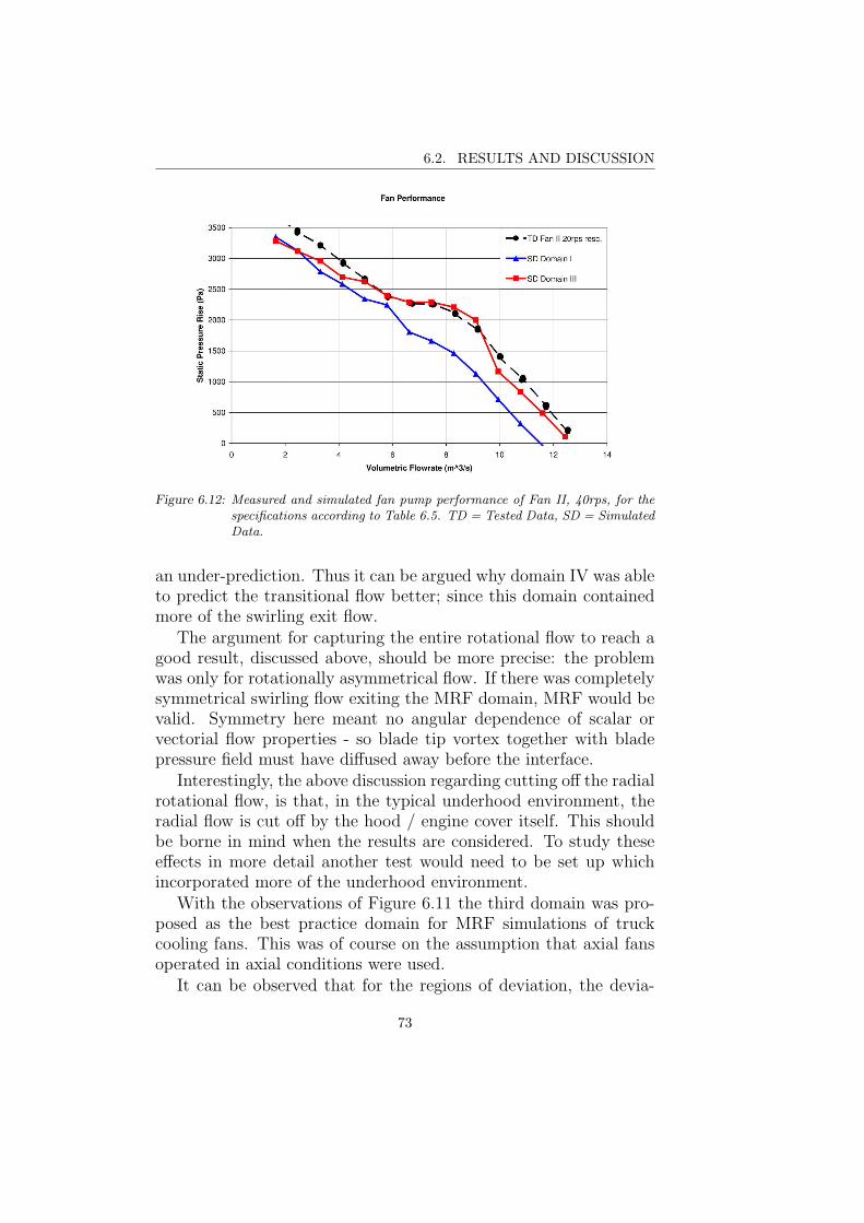
6.2. RESULTS AND DISCUSSION
Figure 6.12: Measured and simulated fan pump performance of Fan II, 40rps, for thespecifications according to Table 6.5. TD = Tested Data, SD = SimulatedData.
an under-prediction. Thus it can be argued why domain IV was ableto predict the transitional flow better; since this domain containedmore of the swirling exit flow.
The argument for capturing the entire rotational flow to reach agood result, discussed above, should be more precise: the problemwas only for rotationally asymmetrical flow. If there was completelysymmetrical swirling flow exiting the MRF domain, MRF would bevalid. Symmetry here meant no angular dependence of scalar orvectorial flow properties - so blade tip vortex together with bladepressure field must have diffused away before the interface.
Interestingly, the above discussion regarding cutting off the radialrotational flow, is that, in the typical underhood environment, theradial flow is cut off by the hood / engine cover itself. This shouldbe borne in mind when the results are considered. To study theseeffects in more detail another test would need to be set up whichincorporated more of the underhood environment.
With the observations of Figure 6.11 the third domain was pro-posed as the best practice domain for MRF simulations of truckcooling fans. This was of course on the assumption that axial fansoperated in axial conditions were used.
It can be observed that for the regions of deviation, the devia-
73

6. FAN MODELLING
Figure 6.13: Measured and simulated fan pump performance of Fan III, 40rps, for thespecifications according to Table 6.5. TD = Tested Data, SD = SimulatedData.
tions for this fan between simulations and measurements started toincrease considerably close to the fan transition region (the knee inthe curve). The fan transition region is a region where the flow outfrom the fan moves from axial flow to radial flow. This is also aregion where the blade can start to stall (flow separates from thesuction side of the blade) and furthermore the tip vortex can bepushed forward of the blade due to the pressure differential acrossthe fan. In essence this is a very turbulent intense flow condition;and the deviations seen in this area could be caused by an infe-rior turbulence models used in this study. Furthermore since thisinvolves blade stalling, this is very sensitive, and there is also thepossibility of interference effects between stationary asymmetricalparts and rotating geometry. This cannot be captured by MRF.
A similar behaviour between domain I and domain III for FanII can be seen in Figure 6.12. It will be seen that domain I under-predicts performance in a similar manner as for Fan I. However, itshould be noted that for the radial flow, the under-prediction is dif-ferent to Fan I, the under-prediction was not a relative increase as itwas for Fan I. Domain III appeared better at capturing the perfor-mance characteristics of axial flow than domain I, but not as goodas for Fan I. Future investigations of the influence of frozen position
74

6.2. RESULTS AND DISCUSSION
Figure 6.14: Measured and simulated fan pump performance of Fan IV, 40rps, for thespecifications according to Table 6.5. TD = Tested Data, SD = SimulatedData.
of the rotor will shed more understanding to why this occured.It should be noted that this fan was one of the two fans that were
deforming during testing, so in this figure the 20rps re-scaled datais presented according to previous discussion in the experimentalsection. Finally, as this fan was an 11-blade one, the transitioncharacteristics was better captured for this fan than for Fan I whichwas an 8-blade one.
For Fan III, Figure 6.13, domain III appeared to accurately pre-dict the axial and transitional characteristics of this fan. Looking atFigures 6.11 - 6.13 the transition characteristics of the 11-blade fansappear to be better captured than for the 8-blade. This could be dueto the constraints of validity of the MRF model was better fulfilledfor the 11-blade fans, since, for the same rotational rate, the flowwas more rotationally uniform across the interface out of the fan,than for the 8-blade fan. The 11-blade fan was more ”continuous”than the 8-blade at the MRF interface.
Finally, Fan III in Figure 6.13 appears to have a slight kink inthe prediction curve mid-section of the axial flow, this can be moreclearly seen in Figure 6.12. And this requires further examination.
For Fan IV, the predictions of domain I in Figure 6.14 followthat of Fan I in Figure 6.11. So, based on these four fans, the error
75

6. FAN MODELLING
Figure 6.15: Velocity magnitude in a plane perpendicular to the axis of rotation, tan-gent to the fan ring, magnified around two blades for domain I.
caused by MRF was consistent for fans of different design, at leastfor the axial flow conditions of these fans.
To further examine the error of the MRF model, it was decidedto simulate a second speed, 20rps for domain I, Fan I, see Table 6.6,and correlate the two simulations using the fan laws. The resultsfrom this are presented in Figure 6.17.
It can be seen in Figure 6.17 that, although the MRF modelseverly under-predicted the fan performance in domain I, see Figure6.11, the error was consistant with an inertial formulation. This canbe observed by the fact that the fan laws work perfectly by scalingin Figure 6.17. Thus the fan laws can be applied to the erroneouslypredicted MRF data, and using the fan laws, apply a speed scaling,and thereby measure the error of the prediction. The results of thisfor domain I and II and for the Fans I, II and IV, can be seen Figures6.18 - 6.21.
Interestingly, for axial flow the domain specification was rela-tively consistent in its prediction of fan performance. For DomainI, a speed correction of 14% allowed the predicted and measuredperformance to align for axial flow conditions. This is verified in
76

6.2. RESULTS AND DISCUSSION
Figure 6.16: Velocity magnitude in a plane perpendicular to the axis of rotation, tan-gent to the fan ring, magnified around two blades for domain II.
Figure 6.18, 6.20 and 6.21. Referring to the method section thisfactor also became the measure of error of the MRF model for axialflow conditions.
Doing the same for Domain II, the under-prediction becomes 8%,see Figure 6.19.
Influence of Fan Frozen PositionNext, domain III, was used to investigate the influence of the
frozen position of the fan. For Fan I and II carrying out the proposedsimulations of Table 6.7 gave the results in Figures 6.22 and 6.23.
It can be seen that: the MRF model holds the fan frozen in its co-ordinate system relative to the inertial frame. Since the constraintsof validity for the MRF model could not be fulfilled for this type ofsimulation, there was an unsteady interaction between the enginesilhouette and the fan. The fan frozen position caused differencesto the predicted fan performance.
In Figures 6.22 and 6.23 it can be seen that for axial flow con-ditions the predictions of pump performance was different for thedifferent frozen positions of the fan. It is interesting to note that it
77
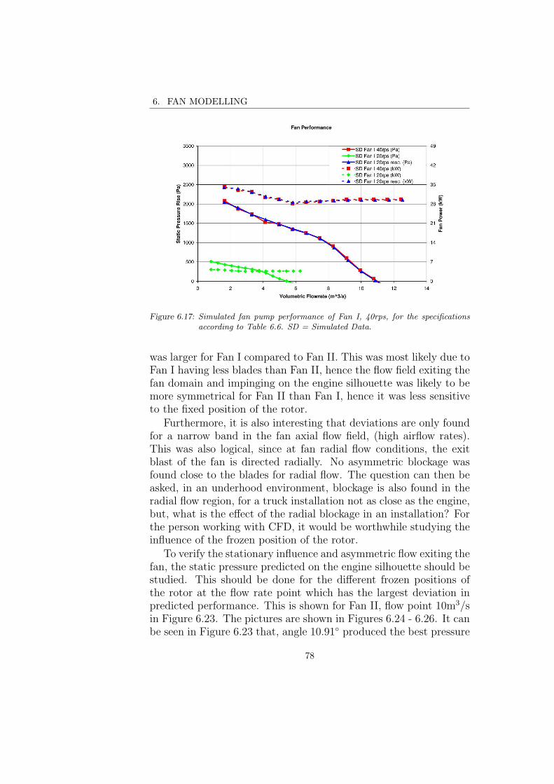
6. FAN MODELLING
Figure 6.17: Simulated fan pump performance of Fan I, 40rps, for the specificationsaccording to Table 6.6. SD = Simulated Data.
was larger for Fan I compared to Fan II. This was most likely due toFan I having less blades than Fan II, hence the flow field exiting thefan domain and impinging on the engine silhouette was likely to bemore symmetrical for Fan II than Fan I, hence it was less sensitiveto the fixed position of the rotor.
Furthermore, it is also interesting that deviations are only foundfor a narrow band in the fan axial flow field, (high airflow rates).This was also logical, since at fan radial flow conditions, the exitblast of the fan is directed radially. No asymmetric blockage wasfound close to the blades for radial flow. The question can then beasked, in an underhood environment, blockage is also found in theradial flow region, for a truck installation not as close as the engine,but, what is the effect of the radial blockage in an installation? Forthe person working with CFD, it would be worthwhile studying theinfluence of the frozen position of the rotor.
To verify the stationary influence and asymmetric flow exiting thefan, the static pressure predicted on the engine silhouette should bestudied. This should be done for the different frozen positions ofthe rotor at the flow rate point which has the largest deviation inpredicted performance. This is shown for Fan II, flow point 10m3/sin Figure 6.23. The pictures are shown in Figures 6.24 - 6.26. It canbe seen in Figure 6.23 that, angle 10.91◦ produced the best pressure
78

6.2. RESULTS AND DISCUSSION
Figure 6.18: Measured, simulated and speed corrected fan pump performance of FanI, 40rps, for domain I. TD = Tested Data, SD = Simulated Data. Thecorrection factor is 14%.
rise, 0◦ the worst, while 21.82◦ produced average amount of pressure.Examining the static pressure on the engine mock-up it can be
verified that the static pressure for 10.91◦ (Figure 6.25) is lower thanfor 21.82◦ (Figure 6.26). And more significantly 21.82◦ had a lowerback pressure on the engine mock-up than 0◦, Figure 6.24. Thus itcan be seen why the fan performance varied with the MRF modelaccording to the choice of frozen position of the rotor; there is astrong interaction between the frozen position of the blade and thestationary engine. At different blade positions, different parts of thefan blade was blocked or covered by the engine, and this caused aback pressure on the fan blade which lowered the total fan pumpperformance prediction. This means that the fan pressure rise ispartly lost to overcome the back pressure caused by the engine.
For reference, the frozen position examination was for Fan I alsocarried out for domain I. It can be seen here that, for this domain,the frozen position was not of major influence. The MRF error wasfar larger and the effect of unsteady interaction between blade andmock-up appeared to be washed away.
It is also of note that in Figures 6.22 - 6.23 the regions of devi-ations, these regions were still bounded to the experimental data.From this it would be of interest to investigate how an average of
79

6. FAN MODELLING
Figure 6.19: Measured, simulated and speed corrected fan pump performance of Fan I,40rps, for domain II. TD = Tested Data, SD = Simulated Data. Thecorrection factor is 8%.
the three predictions would behave. This is presented for Fan I inFigure 6.27 and for Fan II in Figure 6.28.
From Figure 6.27 and 6.28 it will be seen that the simple averageof the three different positions of the fan produced a remarkablygood pressure prediction of the fan. This should be considered asa possible solution if MRF predictions have to be run but there arestrong interaction between the fan blade and stationary objects inthe close vicinity of the MRF domain.
Influence of Turbulence Models and Computational GridThe standard turbulence model for this study was Realizable k-
epsilon. But for the purposes of investigating the influence of thisuser specific choice of turbulence model, k-omega SST together withQuadratic k-epsilon was attempted. Figure 6.29 shows the result.
Typically within the automotive industry, Realizable k-epsilon iswell known for predicting turbulent flow rather well, especially thedrag of a passenger car. Though when the wake flow field of thecar is heavily dominated by strong vorticities, or more generally,when the wake field of the car is of interest, k-omega SST can bepreferred by some users. Both of these turbulence models are basedon the linear assumption of Boussinesq. This essentially assumes
80

6.2. RESULTS AND DISCUSSION
Figure 6.20: Measured, simulated and speed corrected fan pump performance of FanII, 40rps, for domain I. TD = Tested Data, SD = Simulated Data. Thecorrection factor is 14%.
isotropic turbulence. So, if anisotropic turbulence is of interest, itcan be argued one needs to go to a non-linear assumption of Boussi-nesq. Quadratic k-epsilon is one of the more popular anisotropicturbulence models.
In Figure 6.29 the predictions of the three different turbulencemodels are presented for MRF domain III and Fan I. It will be seenin this figure that there was a very low influence from the choice ofturbulence model on the results. Comparing the differences seen inFigure 6.29 to the difference due to the choice of domain specifiedin Figure 6.11, or the frozen position of the rotor, Figure 6.22, theinfluence of the turbulence model is clearly less than the influenceof the fan model itself.
Carrying out the mesh study according to Table 6.8, the resultsin Figure 6.30 were obtained. It is indicated in this figure thatthe default mesh had reached mesh independency. This had almostalready been reached by the coarse mesh, and furthermore it canbe seen in Figure 6.30 that the dependency of mesh resolution isfar smaller than the dependency of frozen rotor position. This canbe seen by comparing the mesh dependency for the flow rate point7.44 m3/s with the variation of frozen position for 11.6 m3/s. Sincethe lower flow rate point converged, the variation of higher flow rate
81

6. FAN MODELLING
Figure 6.21: Measured, simulated and speed corrected fan pump performance of FanIV, 40rps, for domain I. TD = Tested Data, SD = Simulated Data. Thecorrection factor is 14%.
point is most likely caused by unsteady flow physics, not the meshresolution. This can be seen by comparing the variation for thedifferent meshes with the variation of fan frozen position.
Prediction of Fan Power ConsumptionThe previous sections focused on predictions of fan pump per-
formance. This was because fan pump performance was of primaryconcern regarding cooling performance simulations. The secondaryvariable was fan power consumption. For reference, this sectionpresents the predictions of fan power consumption according to thespecification in Table 6.7, but only for the proposed best practicedomain, domain III. Carrying out the simulations according to Table6.7 and extracting fan pump performance and fan power consump-tion gave the results in Figures 6.31 and 6.32. The correspondingaverage data is presented in Figures 6.33 and 6.34.
It can be seen that although the fan pump performance was pre-dicted accurately (for axial flow), fan power consumption was not.Fan power consumption was under-predicted. It can also be seenthat the influence of the frozen position of the rotor was not asstrong for fan power consumption as it was for fan pump perfor-mance.
82

6.2. RESULTS AND DISCUSSION
Figure 6.22: Measured and simulated fan pump performance characteristics of Fan I,40rps, for domain I and III. TD = Tested Data, SD = Simulated Data.
The under-prediction of fan power consumption warrants furtherinvestigation, the following section gives more details.
LBM Investigations
The final part of the fan modelling examination was to study thefan sliding mesh model and compare it to the MRF model. Thiswas carried out in PowerFLOW. Using the set-ups detailed in Table6.9, the results are shown in Figure 6.35 - 6.37.
Starting with Figure 6.35, a clear difference can be seen betweenthe fan performance predictions of these two simulation techniques.The SM method clearly out-performed the MRF approach in corre-lating the fan pressure rise characteristics with experimental data.Furthermore, the SM technique exhibited a remarkable capabilityof accurately capturing almost the entire experimental fan perfor-mance curve in Figure 6.35. Some deviation from experiment canbe noted only for the lowest flow rate point and some deviations canbe seen in fan power consumption predictions, for high flow rates.This will be discussed later.
From one perspective it is somewhat misleading to label SM andMRF as fan models. That characterisation applies to the BFM,where one actually models the fan contribution to the flow with-
83

6. FAN MODELLING
Figure 6.23: Measured and simulated fan pump performance characteristics of Fan II,40rps, for domain III. TD = Tested Data, SD = Simulated Data.
out having a geometrical representation of the fan. MRF on theother hand is a purely mathematical model of a rotating geometryin CFD, which in this case happened to be a fan. Under certainmathematical constraints the MRF technique can be used to modelrotating geometry without that geometry actually moving its po-sition relative to stationary parts. MRF could be more correctlyviewed as a Rotational Model. The SM approach does not makeany modelling assumptions. The rotating parts truly rotate as thesimulation progresses in time. So from this perspective, one shouldnot really call SM a fan model or a rotational model.
This does not however automatically guarantee good results fromthe SM technique when trying to simulate rotational effects or com-ponents. The computational interface between the rotating and non-rotating domains requires careful treatment in order to avoid issuesthat can otherwise arise with the SM approach. The surface ele-ments in these regions never map one-to-one as they ”slide” againsteach other. The communication between these domains must bemathematically accurate and not introduce numerical diffusion orartifacts. The SM implementation in PowerFLOW appears to meetthese criteria.
Furthermore, capturing the entire fan performance curve requires
84

6.2. RESULTS AND DISCUSSION
Figure 6.24: Static pressure predictions of Fan II 0◦, flow point 10m3/s in Figure 6.23.
a physics solver that can handle highly complex geometry and highlycomplex flow. It must be able to predict the effect of turbulence onmean flow variables such as pressure and velocity, which were themain parameters of interest in Figure 6.35. In order to be able to dothis, the underlying turbulence model needs to predict production,transportation and dissipation of turbulent kinetic energy correctly -without over-predicting or under-predicting. The solver should alsomodel solid surfaces in detail and predict separation points/linesaccurately, or at least to the extent that it does not leave unphysicaltraces on the pressure characteristics.
The physics solver has to be paired with a numerical scheme thatdoes not add errors or numerical diffusion to the solution. This issomewhat easier to achieve in a LBM solver that avoids non-linearPartial Differential Equations (PDEs) unlike the traditional Navier-Stokes solvers. The correlation shown in Figure 6.35 indicates thatthe SM implementation in PowerFLOW is matched by the accuracyof the underlying LBM solver and turbulence model.
Figure 6.35 also presents the correlation of fan power consump-tion, which was another variable of interest as it had a direct influ-
85
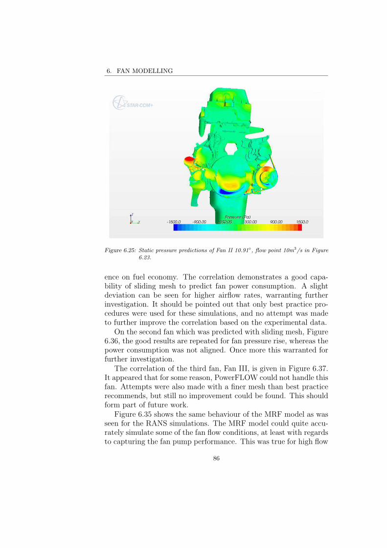
6. FAN MODELLING
Figure 6.25: Static pressure predictions of Fan II 10.91◦, flow point 10m3/s in Figure6.23.
ence on fuel economy. The correlation demonstrates a good capa-bility of sliding mesh to predict fan power consumption. A slightdeviation can be seen for higher airflow rates, warranting furtherinvestigation. It should be pointed out that only best practice pro-cedures were used for these simulations, and no attempt was madeto further improve the correlation based on the experimental data.
On the second fan which was predicted with sliding mesh, Figure6.36, the good results are repeated for fan pressure rise, whereas thepower consumption was not aligned. Once more this warranted forfurther investigation.
The correlation of the third fan, Fan III, is given in Figure 6.37.It appeared that for some reason, PowerFLOW could not handle thisfan. Attempts were also made with a finer mesh than best practicerecommends, but still no improvement could be found. This shouldform part of future work.
Figure 6.35 shows the same behaviour of the MRF model as wasseen for the RANS simulations. The MRF model could quite accu-rately simulate some of the fan flow conditions, at least with regardsto capturing the fan pump performance. This was true for high flow
86

6.2. RESULTS AND DISCUSSION
Figure 6.26: Static pressure predictions of Fan II 21.82◦, flow point 10m3/s in Figure6.23.
conditions, flow rates above 8m3/s, as seen in Figure 6.35. For therest of the curve, a slight under-prediction of performance can beseen, but still the results were reasonably close to the experimentalones.
This indicated that the MRF technique could still offer suffi-cient capability of predicting fan pressure rise characteristics suit-able for cooling performance calculations. For such calculations tobe accurate, it would be necessary to accurately predict fan pumpperformance, since this controls cooling airflow through the heatexchangers, but only over the operating range of the fan for the par-ticular vehicle under construction. For moderate to low restrictioninstallations, the fan would be expected to operate mostly in theaxial, high flow regime and here the MRF model predicts well. It isalso important to note that the error between MRF predictions andexperiments may have depended on the fan geometry and down-stream blockage, and therefore could vary from one fan installationto another.
Figure 6.35 also shows the same behaviour of the fan power con-sumption predictions as was seen for the RANS simulations: the
87

6. FAN MODELLING
Figure 6.27: Measured and simulated average fan pump performance characteristics ofFan I, 40rps, for domain III. TD = Tested Data, SD = Simulated Data.
MRF model under-predicted fan power consumption. Parts of thisunder-prediction is removed by implementing SM in Figure 6.35,however, it is indicated in Figure 6.36, that a complete correlationof fan power consumption has not been established. This warrantsfor further investigations.
It was seen in the previous RANS examination, that the frozenposition of the rotor had a significant influence on predicted fanpressure rise. This was found for the axial flow domain where therewas a strong interaction between the fan and engine mock-up. ForFan I, the deviations were found to be largest for the flow rate of9.11m3/s in Figure 6.22. For this study, it was investigated if thischaracteristic was carried through to the transient MRF simulations.For this examination three different frozen positions of the rotor weresimulated for the most sensitive flow rate point of 9.11m3/s. Theresults are shown in Figure 6.38.
It can be seen that the MRFmodel exhibited a dependency on thefrozen rotor position even here, compared to the stationary RANSsolver, Figure 6.22, for the flow rate point investigated the depen-dency in the LBM solver was found to be weaker, but present. Afull investigation should be carried out, but the results indicated ahigh level of consistency between the fan MRF model implemented
88
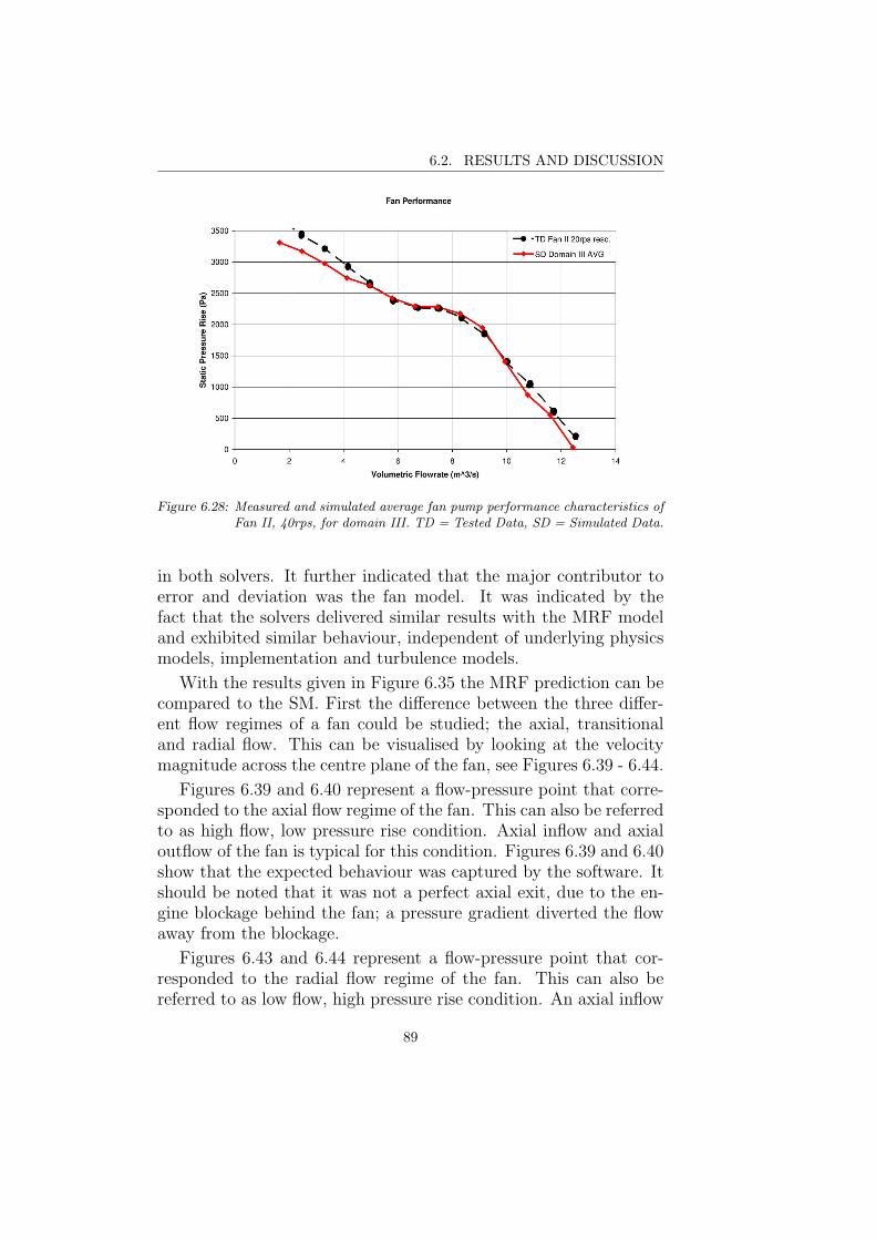
6.2. RESULTS AND DISCUSSION
Figure 6.28: Measured and simulated average fan pump performance characteristics ofFan II, 40rps, for domain III. TD = Tested Data, SD = Simulated Data.
in both solvers. It further indicated that the major contributor toerror and deviation was the fan model. It was indicated by thefact that the solvers delivered similar results with the MRF modeland exhibited similar behaviour, independent of underlying physicsmodels, implementation and turbulence models.
With the results given in Figure 6.35 the MRF prediction can becompared to the SM. First the difference between the three differ-ent flow regimes of a fan could be studied; the axial, transitionaland radial flow. This can be visualised by looking at the velocitymagnitude across the centre plane of the fan, see Figures 6.39 - 6.44.
Figures 6.39 and 6.40 represent a flow-pressure point that corre-sponded to the axial flow regime of the fan. This can also be referredto as high flow, low pressure rise condition. Axial inflow and axialoutflow of the fan is typical for this condition. Figures 6.39 and 6.40show that the expected behaviour was captured by the software. Itshould be noted that it was not a perfect axial exit, due to the en-gine blockage behind the fan; a pressure gradient diverted the flowaway from the blockage.
Figures 6.43 and 6.44 represent a flow-pressure point that cor-responded to the radial flow regime of the fan. This can also bereferred to as low flow, high pressure rise condition. An axial inflow
89

6. FAN MODELLING
Figure 6.29: Measured and simulated fan pump performance characteristics of Fan I,40rps, for domain III and three different turbulence models. TD = TestedData, SD = Simulated Data, RKE = Realizable k-epsilon, QuadKE =quadratic k-espilon and KWsst k-omega sst.
and radial outflow of the fan are typical of this condition. It can beseen clearly in Figures 6.43 and 6.44 that the flow attached radiallyto the rig wall. Another characteristic of this flow regime was thatthe high pressure gradient over the fan pushed the blade trailingvortex forward, and a re-circulation path was created over the fanthat extended into the pressure chamber. Traces of this can also beseen in Figures 6.43 and 6.44.
Finally, Figures 6.41 and 6.42 illustrate a flow point that wasin the middle of the fan transition regime. This was the transitionbetween radial and axial flow. This can be a violent transition andthis can be seen to some extent in the figure.
For reference, comparative flow images are shown for MRF andSM simulations. Visual differences of the flow paths obtained usingthe two methods can be seen, but nothing that illustrates why theMRF falls short of the SM. This should be investigated further.One indication can be seen in the figures when comparing MRF toSM, the dynamic pressure exiting the fan, and also re-circulating,appears to be larger for the MRF than SM (indicated by larger redareas exiting the fan). But this must be investigated more closely.
The reason the MRF model fell short in predicting fan perfor-
90

6.2. RESULTS AND DISCUSSION
Figure 6.30: Measured and simulated fan pump performance characteristics of Fan I,40rps, for domain III, two flow rate points of 11.6 m3/s and 7.44 m3/sand four different meshes according to Table 6.8. TD = Tested Data, SD= Simulated Data.
mance, whereas SM did not, can be discussed and understood fromseveral perspectives. The simplest being that the absence of pureaxis-symmetric flow across the MRF domain caused this. From thetheory chapter, the MRF model needed steady state flow across theinterface in both frames of reference to be mathematically correct,and it was the absence of this that was the cause of the deviation.This could partly be caused by a too small domain, or the vicinityof non-rotationally symmetric objects close to the fan (the squarefan shroud upstream, and engine mock-up downstream). In essenceit was the unsteady flow that violated the constraints of the model.This however does not explain the fact that the MRF model pre-dicted axial flow, but not transitional or radial airflow. Furthermoreit does not explain why some domains under-predicted fan perfor-mance more severely than others.
Instead it may be appropriate to decompose the fan airflow andmomentum into axial flow, tangential flow and radial flow. The ax-ial flow through the fan is proportional to the volumetric flow rate,the X-axis in the performance curves. The tangential flow exiting
91

6. FAN MODELLING
Figure 6.31: Measured and simulated fan pump performance characteristics and fanpower consumption of Fan I, 40rps, for domain III. TD = Tested Data,SD = Simulated Data.
the fan is proportional to fan rpm, hence it is constant in the per-formance curve. The radial flow can be obtained from conservationof mass and momentum. Thus, at higher flow rates, rotational ef-fects are relatively less significant for pressure rise: it is the axialflow that determines the pumping performance. At lower flow rates,rotational effects dominate over axial flow, and these effects do notseem to be captured with MRF for this type of asymmetric testset-up.
It can be seen in Figures 6.39 and 6.40 that there was a smoothflow into the fan, whereas the exit impinged and interacted withthe engine mock-up. This impingement could be considered as ablockage with the influence of fan frozen position. Most of the axialand swirling exit momentum was converted to radial momentumwhich was later lost, since there was not a diffuser that recoveredthis dynamic pressure. Hence, other than the actual axial pressureblockage of the mock-up, no influence on static pressure rise was left.For this flow condition the entire swirling energy was captured andcontained within the MRF domain. This also followed the previousRANS observations. Domain III contained the swirling flow betweenthe fan and engine. Domain I and II did not, and it was also foundthat these domains under-predicted axial fan performance.
92

6.2. RESULTS AND DISCUSSION
Figure 6.32: Measured and simulated fan pump performance characteristics and fanpower consumption of Fan II, 40rps, for domain III. TD = Tested Data,SD = Simulated Data.
Examining Figures 6.43 and 6.44, the flow into the fan was notsmooth, whereas the exit flow was radial and only interacted withthe engine mock-up to a weak extent. Thus, for this flow conditionthe blade tip over-flow was pushed upstream into the pressure cham-ber. This meant there was swirling flow that was transported up-stream, crossing the MRF interface and re-circulated back throughthe fan. This swirling flow contained energy which had been sup-plied by the fan, and the re-circulation of this can potentially beimportant for the overall prediction of fan performance. Further-more this re-circulation tends to distort the flow going into the fan,and this will influence fan performance. At the exit, the swirlingflow exited the fan in a radial direction. And similar to the inletside - the swirl crossed the MRF boundary here. For these flow con-ditions the simulation under-predicted performance. To summarise,two effects were identified; For axial flow, where the effect of swirlis relatively less important for prediction of static pressure rise, andthe entire swirling energy was kept within the MRF domain, a goodprediction was achieved by the simulations. In contrast, when theeffect of swirl was of importance for pressure prediction and it wastransported across the MRF domain, the model under-predictedperformance. This indicated that the MRF model either had diffi-
93
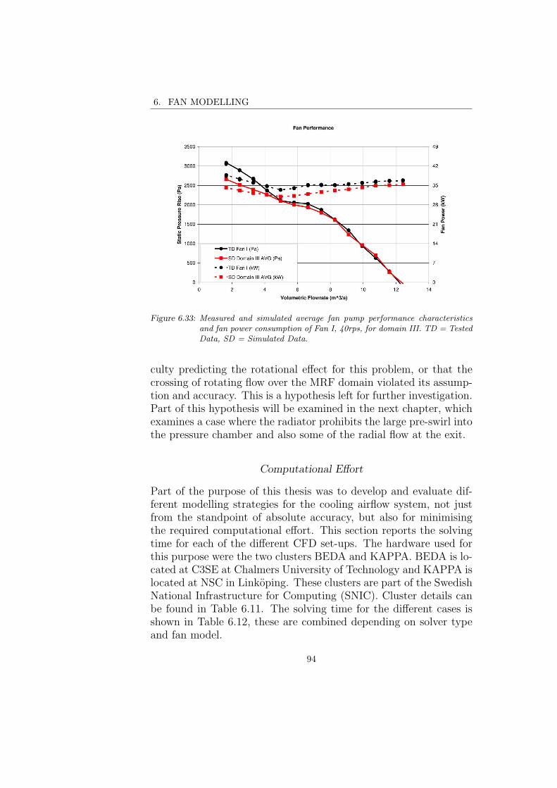
6. FAN MODELLING
Figure 6.33: Measured and simulated average fan pump performance characteristicsand fan power consumption of Fan I, 40rps, for domain III. TD = TestedData, SD = Simulated Data.
culty predicting the rotational effect for this problem, or that thecrossing of rotating flow over the MRF domain violated its assump-tion and accuracy. This is a hypothesis left for further investigation.Part of this hypothesis will be examined in the next chapter, whichexamines a case where the radiator prohibits the large pre-swirl intothe pressure chamber and also some of the radial flow at the exit.
Computational Effort
Part of the purpose of this thesis was to develop and evaluate dif-ferent modelling strategies for the cooling airflow system, not justfrom the standpoint of absolute accuracy, but also for minimisingthe required computational effort. This section reports the solvingtime for each of the different CFD set-ups. The hardware used forthis purpose were the two clusters BEDA and KAPPA. BEDA is lo-cated at C3SE at Chalmers University of Technology and KAPPA islocated at NSC in Linkoping. These clusters are part of the SwedishNational Infrastructure for Computing (SNIC). Cluster details canbe found in Table 6.11. The solving time for the different cases isshown in Table 6.12, these are combined depending on solver typeand fan model.
94

6.2. RESULTS AND DISCUSSION
Figure 6.34: Measured and simulated average fan pump performance characteristicsand fan power consumption of Fan II, 40rps, for domain III. TD = TestedData, SD = Simulated Data.
In Table 6.12 it can be seen that there was some spread tothe computational requirements even within the same solver. Thisspread was mainly caused by the differences in case size (elementcount) and the flow physics that was being solved (some flow pointswere less stable and required longer solving time to reach conver-gence).
Table 6.12 shows some differences in solving time between solver.It can be seen that in general the RANS based solver required lesscomputational effort to converge a MRF simulation than the LBMsolver. This was expected since RANS is a steady state formulationof fluid flow, whereas the LBM has a transient formulation in thepresent solver.
It can also be seen that SM required more computational effortthan MRF. This was also expected, the extra effort comes fromcomputing the connection between stationary and moving cells atthe sliding interface, see the theory chapter for details, section 2.2.2Fan Models.
95

6. FAN MODELLING
Figure 6.35: Measured and simulated fan pump performance of Fan I, 40rps, for thespecifications according to Table 6.9. TD = Tested Data, SD = SimulatedData.
6.3 Intermediate Summary and Conclusions
In this chapter fan modelling strategies have been examined. Thetwo models of MRF and SM were applied for a test case that incor-porated four different truck fans, shroud, ring and engine mock-up.Furthermore two differerent CFD solvers have been examined.
This study has found that the MRF have good capabilities forpredicting the fan pump performance of axial fan airflow. For somefans this even extends into the transition.
Also documented was the sensitivity of the MRF model to theuser specific choice of rotational domain and also frozen position ofthe rotor. These two dependencies were the most severe constraintsfor prediction accuracy. So a best practice procedure of domainchoice was proposed, and for cases where there was a strong inter-action between the frozen position of the rotor and fan performancea method to check and deal with these was proposed.
Finally the influence of SM model compared to MRF for a LBMsolver was studied. This solver has a more rigid form of turbulencemodel than the RANS code. This solver is also transient. Andfor these purposes the MRF model predicted the same performanceas the RANS solver. Whereas the SM model predicted extremely
96
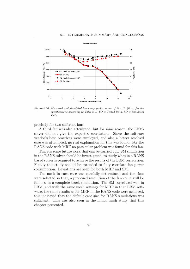
6.3. INTERMEDIATE SUMMARY AND CONCLUSIONS
Figure 6.36: Measured and simulated fan pump performance of Fan II, 40rps, for thespecifications according to Table 6.9. TD = Tested Data, SD = SimulatedData.
precisely for two different fans.A third fan was also attempted, but for some reason, the LBM-
solver did not give the expected correlation. Since the softwarevendor’s best practices were employed, and also a better resolvedcase was attempted, no real explanation for this was found. For theRANS code with MRF no particular problem was found for this fan.
There is some future work that can be carried out. SM simulationin the RANS solver should be investigated, to study what in a RANSbased solver is required to achieve the results of the LBM correlation.Finally this study should be extended to fully correlate fan powerconsumption. Deviations are seen for both MRF and SM.
The mesh in each case was carefully determined, and the sizeswere selected so that, a proposed resolution of the fan could still befulfilled in a complete truck simulation. The SM correlated well inLBM, and with the same mesh settings for MRF in that LBM soft-ware, the same results as for MRF in the RANS code were achieved,this indicated that the default case size for RANS simulations wassufficient. This was also seen in the minor mesh study that thischapter presented.
97

6. FAN MODELLING
Figure 6.37: Measured and simulated fan pump performance of Fan III, 40rps, for thespecifications according to Table 6.9. TD = Tested Data, SD = SimulatedData.
Figure 6.38: Measured and simulated fan pump performance of Fan I, 40rps, for thespecifications according to Table 6.9 and three frozen positions of the rotor.TD = Tested Data, SD = Simulated Data.
98

6.3. INTERMEDIATE SUMMARY AND CONCLUSIONS
Figure 6.39: Velocity magnitude visuali-sation through fan centre-line at 9.93 m3/s. SM.
Figure 6.40: Velocity magnitude visuali-sation through fan centre-line at 9.93 m3/s. MRF.
Figure 6.41: Velocity magnitude visuali-sation through fan centre-line at 6.62 m3/s. SM.
Figure 6.42: Velocity magnitude visuali-sation through fan centre-line at 6.62 m3/s. MRF.
99
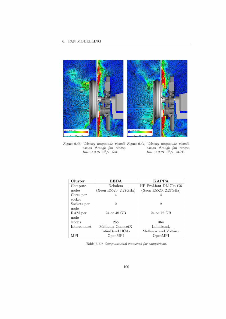
6. FAN MODELLING
Figure 6.43: Velocity magnitude visuali-sation through fan centre-line at 3.31 m3/s. SM.
Figure 6.44: Velocity magnitude visuali-sation through fan centre-line at 3.31 m3/s. MRF.
Cluster BEDA KAPPACompute Nehalem HP ProLiant DL170h G6nodes (Xeon E5520, 2.27GHz) (Xeon E5520, 2.27GHz)Cores per 4 4socketSockets per 2 2nodeRAM per 24 or 48 GB 24 or 72 GBnodeNodes 268 364Interconnect Mellanox ConnectX Infiniband,
InfiniBand HCAs Mellanox and VoltaireMPI OpenMPI OpenMPI
Table 6.11: Computational resources for comparison.
100

6.3. INTERMEDIATE SUMMARY AND CONCLUSIONS
Solver Fan Model Solving TimeRANS MRF 200 - 400 CPU-hLBM MRF 6000 - 7000 CPU-hLBM SM 8000 - 9000 CPU-h
Table 6.12: Computational effort, CPU-h is the equivalent of 1 hour’s worth of 100%CPU time gone to one program.
101

6. FAN MODELLING
102

7. ISOTHERMAL COOLING AIRFLOW SYSTEMMODELLING
7.1 Method
The last part of this thesis takes the information from the two previ-ous chapters of heat exchanger and fan modelling and applies themto a composite system model.
For this a third test set-up was constructed. This test set-upplaced a production fan inside a production fan ring. In front ofthe fan ring a production square fan shroud together with a waterradiator was placed, and after the fan a 2D engine silhouette wasplaced together with a hood that covered the top and sides of theinstallation. See Figure 7.1 for the test set-up. In this test set-upthe radiator front face was aligned with the wall that separated theinlet plenum and outlet plenum.
As previously the fan ring was connected by a rubber seal to thefan shroud.
For this set-up, production parts were used for the fan, shroud,ring, seal and water radiator. For the mock-up a 2D silhouette wascut from a wooden board. This was also modeled in CFD.
This set-up was only used for one fan, Fan I, and one heatexchanger. This set-up was not only correlated on the predictedplenum pressure difference in the rig, but also for the local velocityin the radiator, measured with 48 velocity probes.
7.1.1 Experimental Measurements
The experimental study was carried out in the Volvo 3P Fan TestRig, described in Section 2.1. And tests were set up according toFigure 7.1.
For these experiments the static pressure was measured betweenthe two chambers as a function of different volumetric flow rates,for a fixed fan speed of 40rps.
103

7. ISOTHERMAL COOLING AIRFLOW SYSTEM MODELLING
Figure 7.1: Set-up of system modelling examination.
During testing, fan power consumption was also measured. Thedetails of this are presented in Appendix A.1 Measuring Fan Power.Also during testing the radiator was fitted with 48 Microprobes asdescribed in Section 2.1.1 Velocity Measurements Across Radiator.
All data was later presented at standard air conditions. Theprocedure to reach standardised outputs is described in AppendixA.1 Standard Air Conditions.
The microprobe system was calibrated by mounting the radiatorwith the inlet duct according to Figure 5.1, and sweeping a rangeof flow rates through the test rig. After this, the calibration waschecked. At the end of the test sequence the microprobe calibrationwas once more checked. Table 7.1 summarises all the steps in thetest procedure.
Test step Description1 Calibration of Microprobe system2 Check calibration of Microprobe system3 Run system test and measure local velocities4 Re-check calibration of Microprobe system
Table 7.1: Steps for the system test.
104

7.1. METHOD
7.1.2 Numerical Simulations
The computational part of this study utilised StarCCM+ version5.06.010. For the test set-up a CAD model of the pressure chamberand outlet chamber was created. Details can be seen in Figure 5.5.
The aim of the numerical test rig was to incorporate a veloc-ity inlet condition at the inlet face to the pressure chamber. Bypre-scribing the inlet velocity, the volumetric flow rate was set. Fur-thermore the outlet chamber was maintained at ambient pressure byprescribing a pressure outlet boundary condition to the outlet faceof the test rig. By measuring the differential static pressure betweenthe two chambers, in the same positions as for actual test rig, thepressure flow characteristic could be computed.
The main settings in the CFD solver for all cases were as follows:
• This study used 3D incompressible Reynolds Averaged Navier-Stokes equations.
• The segregated solver together with second order discretisationschemes were used.
• The air density was set to standard air conditions (1.2kg/m3).
• Turbulence was modelled using Realizable k-epsilon, two layermodel (shear driven, Wolfstein).
• Walls were modelled using two layer all y+ wall treatment. y+spanned at the majority of surface cells between 30-100.
• Boundary conditions were velocity inlet and pressure outletpositioned to the right and left respectively in Figure 5.5.
• The core of the heat exchanger was modelled as porous me-dia as described in Section 2.2.2 Porous Media. The porouscoefficients were obtained as described in Chapter 5.
• The fan was modelled using the MRF model and the best prac-tice procedure of Chapter 6. Also for this fan, the influence ofthe three different frozen positions of the rotor was examined.
For the correlation of velocity probe measurments, a digital ve-locity probe was used in the same position as of the microprobes.Since the microprobe system can only measure velocity in one di-rection, not recirculation, the numerical probe automatically zeroed
105
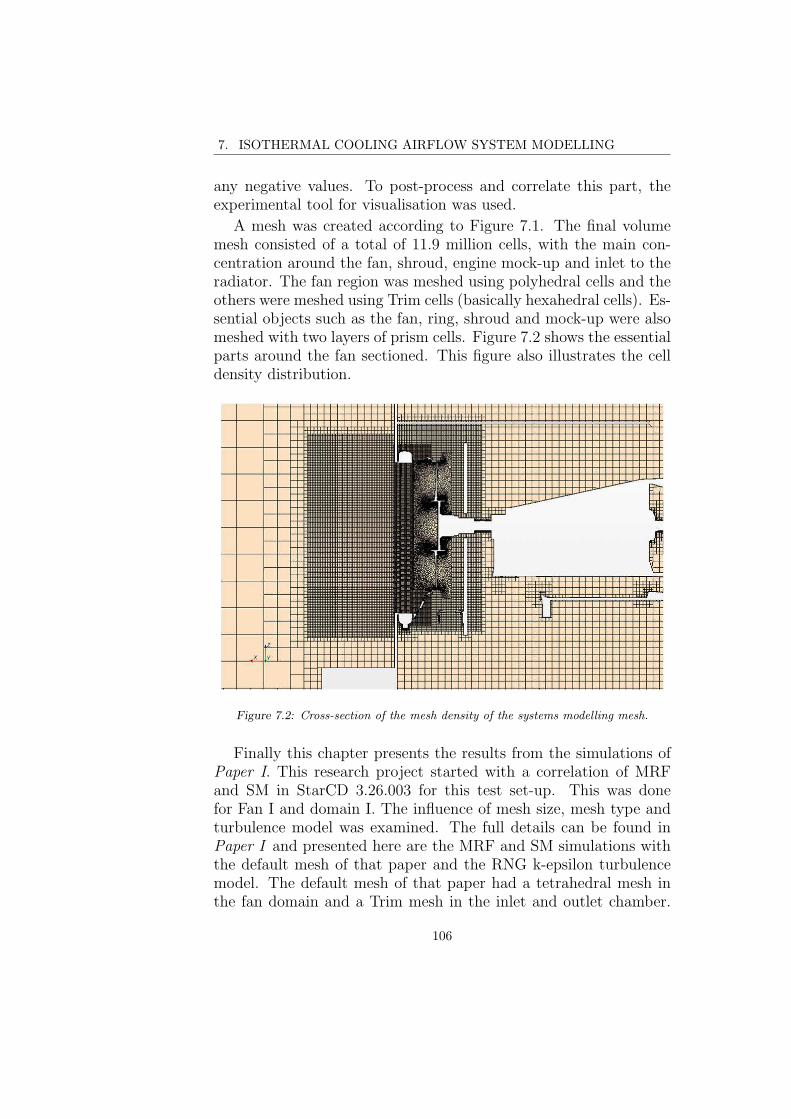
7. ISOTHERMAL COOLING AIRFLOW SYSTEM MODELLING
any negative values. To post-process and correlate this part, theexperimental tool for visualisation was used.
A mesh was created according to Figure 7.1. The final volumemesh consisted of a total of 11.9 million cells, with the main con-centration around the fan, shroud, engine mock-up and inlet to theradiator. The fan region was meshed using polyhedral cells and theothers were meshed using Trim cells (basically hexahedral cells). Es-sential objects such as the fan, ring, shroud and mock-up were alsomeshed with two layers of prism cells. Figure 7.2 shows the essentialparts around the fan sectioned. This figure also illustrates the celldensity distribution.
Figure 7.2: Cross-section of the mesh density of the systems modelling mesh.
Finally this chapter presents the results from the simulations ofPaper I. This research project started with a correlation of MRFand SM in StarCD 3.26.003 for this test set-up. This was donefor Fan I and domain I. The influence of mesh size, mesh type andturbulence model was examined. The full details can be found inPaper I and presented here are the MRF and SM simulations withthe default mesh of that paper and the RNG k-epsilon turbulencemodel. The default mesh of that paper had a tetrahedral mesh inthe fan domain and a Trim mesh in the inlet and outlet chamber.
106

7.2. RESULTS AND DISCUSSION
Compared to the default mesh of this thesis, Figure 7.2, the defaultmesh of Paper I was relatively coarse, it contained 3 million cells.
7.2 Results and Discussion
This part of the study started with calibrating the microprobe sys-tem. The pressure characteristics of the radiator fitted with theprobes was measured, and this data was used to calibrate the porouscoefficients for the CFD model. After the calibration, the calibra-tion was re-checked, and also after the system test, the calibrationwas checked again. The pressure characteristics of these measure-ments, together with a second order polynomial fit of the pressuredrop measurements of the calibration, is shown in Figure 7.3. It canbe seen that the system characteristics repeated itself. Note thatthe test set-up was changed between the calibration and re-checkof calibration but the system gives the same results. It can also beseen that a second order polynomial fits the tested data very well.
Figure 7.3: Plenum pressure drop data of the heat exchanger, TD = Tested Data.
Figure 7.4 shows the differential plenum pressure characteristics.The microprobe system measured the local velocity and these werealso extracted from the CFD simulations. Figure 7.5 shows an exam-ple of the experimental results and Figure 7.6 shows the correlatingsimulation result. Comparing measurements of 48 velocity-probesin this manner is very inefficient. So the statistical measurements
107

7. ISOTHERMAL COOLING AIRFLOW SYSTEM MODELLING
of average velocity through the radiator and also the standard de-viation of radiator velocity is given in Figure 7.7 and 7.8.
Figure 7.4: Measurement of plenum pressure drop correlated with simulated plenumpressure drop. TD = Tested Data, SD = Simulated Data.
It can be seen in Figure 7.4 that three distinct regions can beidentified: A high airflow region with good correlation of plenumpressure rise; An intermediate region with poor correlation; And alow flow rate region, where the prediction slowly recovers. Thesethree regions actually correlates rather well with the prediction seenin the previous chapter and Figure 6.27. In the previous chapter itwas concluded that the best practice procedure could be used for fanaxial flow condition, with extra care required during fan transitionbut not for fan radial flow. This is also what is seen in Figure 7.4.Comparing Figure 7.4 to Figure 6.27 the regions of correlation anddeviation match reasonably well when considering the volumetricflow rates. Note that the mock-up was different between the two,so that an exact correlation could not be expected, but the sametrends are exhibited. Furthermore, since the radiator was included,there was an associated pressure drop in this component, explainingwhy the pressure signals are different between the two graphs.
Another very interesting point was the behaviour of the fan frozenposition. In Figure 7.4 this behaviour is almost completely absent.This is likely to be due to two facts: The first being that for thistest, the non-symmetric mock-up was moved further away from thefan than for the first test case, this means that the interaction was
108

7.2. RESULTS AND DISCUSSION
Figure 7.5: Velocity Measurements through the heat exchanger for 12m3/s, TestedData.
not expected to be as strong as of the previous chapter; secondly,the MRF model was not tangent to the mock-up. Note that theMRF model did not extend all the way to the engine mock-up.This is likely to disconnect some of the strong influence in a similarmanner as was seen for domain I and III in Figure 6.22. It wouldbe interesting to look into a similar MRF domain study of this case,and also to repeat the tests and simulations with the 3D silhouetteof the previous chapter and consider how this correlates. So far thishas not been covered by this research project.
Comparing the results in this part of the study, the MRF modeldid not seem to capture the behaviour of fan transition and stall, butit is interesting that it does not correlate to the previous chapter; theMRF model slowly recovers the prediction at low flow rates. Thiswas not seen in the previous fan work. It was most likely due to theplacement of the water radiator, and the fact that this inhibited thepre-rotation of flow for stalled flow conditions, so that it could notpre-rotate as much as for the fan test case. This pre-rotation wasseen way up in the pressure chamber in Figure 6.43.
For the velocity distribution correlation, Figure 7.5 compared toFigure 7.6 shows a rather good correlation between the predictedflow field in CFD compared to that tested. A small difference canbe seen: the velocity gradients are sharper and more pronouncedin CFD compared to the tested data for this point. Importantly
109

7. ISOTHERMAL COOLING AIRFLOW SYSTEM MODELLING
Figure 7.6: Measurements through the heat exchanger for 12m3/s, Simulated Data.
though the main physics was captured; one can clearly see a higherflow rate around the location of the fan and fan blades, and lowervelocities around the perimeter of the radiator. The fan centre didnot coincide with the centre of the radiator. The fan centre wasplaced slightly above the radiator centre, and this can be seen bythe shift of higher velocities to the top of the radiator, Figures 7.5and 7.6.
For the statistical part of this study, the previously seen trendconstitutes: for flow rates above 7m3/s good correlation was foundfor both the average radiator velocity and the standard deviation ofradiator velocity in Figure 7.7 and 7.8. For flow rates below 7m3/sthe correlation was not maintained, and what can be seen in Figure7.8 is that the physics of the transition was not captured at all insimulations. The distribution was completely different. The CFDsimulations predicted a much higher non-uniformity across the heatexchanger than was measured in the test. This is likely to be theexplanation as to why the prediction in Figure 7.4 was inaccuratefor these points: since a large non-uniformity tends to be a sourcefor a higher pressure drop.
Comparing these results to the earliest predictions in StarCD,the results in Figures 7.9 - 7.11 were obtained. It can be seen inFigure 7.9 that MRF domain I under-predicted the system perfor-mance considerably. The only point where domain III gave similarresults as domain I was in the transition point of the fan. It can also
110
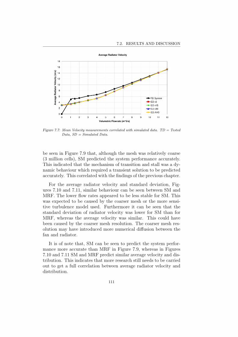
7.2. RESULTS AND DISCUSSION
Figure 7.7: Mean Velocity measurements correlated with simulated data. TD = TestedData, SD = Simulated Data.
be seen in Figure 7.9 that, although the mesh was relatively coarse(3 million cells), SM predicted the system performance accurately.This indicated that the mechanism of transition and stall was a dy-namic behaviour which required a transient solution to be predictedaccurately. This correlated with the findings of the previous chapter.
For the average radiator velocity and standard deviation, Fig-ures 7.10 and 7.11, similar behaviour can be seen between SM andMRF. The lower flow rates appeared to be less stable for SM. Thiswas expected to be caused by the coarser mesh or the more sensi-tive turbulence model used. Furthermore it can be seen that thestandard deviation of radiator velocity was lower for SM than forMRF, whereas the average velocity was similar. This could havebeen caused by the coarser mesh resolution. The coarser mesh res-olution may have introduced more numerical diffusion between thefan and radiator.
It is of note that, SM can be seen to predict the system perfor-mance more accurate than MRF in Figure 7.9, whereas in Figures7.10 and 7.11 SM and MRF predict similar average velocity and dis-tribution. This indicates that more research still needs to be carriedout to get a full correlation between average radiator velocity anddistribution.
111

7. ISOTHERMAL COOLING AIRFLOW SYSTEM MODELLING
Figure 7.8: Standard deviation of velocity through heat exchanger, measured result cor-related to simulated data. TD = Tested Data, SD = Simulated Data.
7.3 Intermediate Summary and Conclusions
In this chapter cooling airflow system modelling strategies have beenexamined. It can be concluded that the observations of fan and heatexchanger modelling of the previous chapters has consistently beencarried over to the composite system model. Good prediction wasfound when the system operates in fan axial flow conditions, andthis was where the fan model was documented to be functioning.Furthermore it should be pointed out that no deficiencies in theheat exchanger model were identified in the previous chapters andnone was found in this chapter. This means, all deficiencies weredue to fan modelling.
For fan transitional flow, the system model using MRF did notgive the expected results, and this corresponds to previous chapters.As was also seen in these chapters, the radial flow did not correlate.
This chapter presented the results from SM simulations of thesystem. These simulations used a coarse mesh and it was found thatthe SM had better capabilities to predict fan transition over MRF.This indicated that fan transition is a dynamic event. Even thoughsystem performance was captured more accurately by SM, radiatoraverage velocity and standard deviation was not. SM and MRFcorrelated better to eachother then SM correlated with experiments.This warranted further investigation.
112

7.3. INTERMEDIATE SUMMARY AND CONCLUSIONS
Figure 7.9: Measurement of plenum pressure drop correlated with simulated plenumpressure drop. TD = Tested Data, SD = Simulated Data.
Figure 7.10: Mean Velocity measurements correlated with simulated data. TD = TestedData, SD = Simulated Data.
113

7. ISOTHERMAL COOLING AIRFLOW SYSTEM MODELLING
Figure 7.11: Standard deviation of velocity through heat exchanger, measured resultcorrelated to simulated data. TD = Tested Data, SD = Simulated Data.
114

8. SUMMARY
This thesis presents research of engineering methods and models ofthe the flow process in engine bays. The main focus has been 3Dmodelling of cooling airflow, and this has been researched with thesupport of experimental measurements. All of the results have beencompared on the basis of 1D cooling airflow models.
To briefly recall two of the main points of this thesis:
1. Today, engine thermal management constraints have increased,new engines need to be maintained with increased precision tobecome more efficient.
2. There have been many more components added to the enginebay, so that, evacuating the hot airflow out of the engine bayhas become more critical.
This means that today there is more heat to be evacuated fromthe engine bay and at the same time less space in which to doso. Thus there is the need for detailed 3D optimisation of the flowprocess in engine bays.
After this, the underlying theory that was required for this workwas laid out. Experimental resources were described, a 1D modelof cooling airflow was also described, and later 3D computationalfluid dynamics were explained: detailing the engineering methodsavailable in this field, as well as describing the tools that would beused and developed.
There followed a chapter of Preceding and Contemporary Work,elaborating on work done by others in this field of research. But fordetailed modelling of the entire flow process in CFD, with full 3Drepresentation of the engine bay and its components, including thefan, very little had been published. This illustrated that there wasindeed a need for deeper research and deeper understanding of thisarea.
115

8. SUMMARY
After this there followed three chapters structured to highlightmethods, results, discussions thereof and intermediate conclusions.First, heat exchanger modelling techniques were investigated. Amethod was developed and the physics of using a plenum to plenumtest facility and extracting restriction data to a CFD simulation inan optimal way was explained. With the methods proposed an errorbelow 0.4% in pressure was achieved for a water radiator.
This was followed by a chapter dealing with different aspects of3D fan modelling techniques. In this chapter two fan models wereexamined, the MRF model and SM model. It was found that theSM model delivered good accuracy of predictions. It was also foundthat the MRF model was capable of handling the fan axial flowregime to a certain extent. Furthermore the sensitivity of the MRFmodel was studied and documented. This model was sensitive tothe user specific choice of rotational volume and also to the frozenposition of the rotor in the simulation. This was true for the specifctest cases examined, a characteristic being that they were all veryconstrained from a packaging perspective.
The final chapter dealt with a system model that was composedof a fan and heat exchanger. It was found that the conclusions fromthe first chapters were carried into this part of the work. The heatexchanger model did not cause any concerns, whereas the problemsof the MRF model applied to the system as well. Thus the systemcould predict the fan axial flow conditions well but not transitionalor radial flow. These conclusions were also supported by detailedvelocity measurements through the radiator.
116

9. CONCLUSIONS
The general conclusion that can be drawn is that 3D CFD can beused to model the complete cooling airflow system accurately.
Specific conclusions are that:
• Accurate measurements and control of the measurements of theradiator pressure drop are required. This enables the extractionof the correct coefficients for the porous media model for usein commercial CFD software.
• The fan MRF model can be used to model a fan that is oper-ating in an axial flow regime in an installation. Although careis required with the user specific choice of rotational domain,and also with any interaction between the fan and asymmetricstationary geometry.
• To achieve good correlations over the entire range of fan oper-ating conditions, the fan SM model should be used to model thefan. This fan model, with suitable treatment of turbulence inthe solver, can give an almost exact prediction of performance.
117

9. CONCLUSIONS
118
10. FUTURE WORK
There was some work that was not covered by this thesis. Thefollowing areas are suitable for further study:
• Follow up the system study with highly resolved sliding meshsimulations of the fan model to be able to study any correlation.
• The system study should be complemented with a second testset-up, using the 3D mock-up in similar settings as for the fanstudy, to closer study the correlation.
• The system study should be checked for repeatability.
• Compare the sliding mesh model of a RANS based softwareto the results of the LBM prediction. This should be done todocument how much work is required with a RANS solver toget similar results of that in LBM.
119

10. FUTURE WORK
120
11. SUMMARY OF PAPERS
Paper I
3D Fan Modeling Strategies for Heavy Duty Vehicle Cool-
ing Installations - CFD with Experimental Validation
Presented at FISTIA World Automotive Congress 2008, Munich.
This paper presented the first pieces of work of this research project.The first study examined the prediction of the cooling airflow systemthat were presented in Chapter 7. In this paper the predictions ofthe MRF model with a small domain was compared to predictions ofsliding mesh. Furthermore the influence of turbulence models, meshdependence and empirical data were analyzed to a certain extent.
In this work it was found that it was very difficult to get the fanMRF model to perform well in a complete vehicle installation. It wasfound that this result and conclusion was independent, to a limitedextent, to choice of turbulence model, mesh size and empirical dataused for the heat exchangers. By contrast, fully transient (URANS)sliding mesh approach performed well, even for small case sizes.
In this work, the complete answer could not be given for fanmodelling techniques, limitations of two equation turbulence modelsand wall functions was encountered when it came to flow regimesneeding accurate prediction of separation and recirculation.
Paper II
A Correction Method for Stationary Fan CFD MRF Mod-
els
Presented at SAE World Congress 2009, Detroit.
From paper I, it was found that the MRF model was not succesfulat predicting fan performance. However since the MRF model in
121

11. SUMMARY OF PAPERS
a RANS code was significantly faster than SM in a URANS solverthe research project continued and constructed a fan only test con-dition. This test was constructed so that the MRF model couldbe understood for the purpose and context of truck cooling airflowsimulations. This was the test set-up that was presented in Chapter6.
In the work presented in this paper it was found that the MRFmodel was a consistent model, in that it consistently under-predictedfan performance, and this under-prediction was consistent with thefan inertial laws. Based on this, the error of the MRF model forthe specific choice of domain could be measured and it was found tobe 14% for axial flow conditions. Furthermore this paper presenteda method of correcting the under-prediction by speeding up thefan for these conditions. This method focused on how to predict abetter fan curve with the MRF method. A fan curve being staticpressure rise as function of volumetric flow rate at a fixed fan speed.This paper concentrated on a small circular domain around the fan,according to domain I in Figure 6.2 and this domain was also thedomain used in the previous paper as well.
Paper III
An Investigation and Correction Method of Stationary Fan
CFD MRF Simulations
Presented at Thermal System Efficiencies Summit 2009, Troy.
The research project continued from paper II by looking into theMRF model and how it predicted performance of different fans. Themain task was to examine whether the under-prediction was consis-tent for fans of different designs, and in this paper three differentfans were examined; Fan I, II and IV of Table 6.1. It was foundthat the under-prediction of 14% for fan axial flow conditions wasconsistent across these three fans.
Furthermore in this paper the mathematics of the MRF was stud-ied and an investigation was carried out to extend the MRF domainout to the fan ring, so that one MRF interface was excluded. Thiscorresponds to domain II in Figure 6.2. It was found in this paperthat this domain decreased the under-prediction of fan axial flowconditions to 8%.
122

Paper IV
Continued Study of the Error and Consistency of Fan CFD
MRF Models
Presented at SAE World Congress 2010, Detroit.
In previous papers it was found that the choice of domain had sig-nificant influence on the error of the MRF model. So in this paperthree different domains were invesigated for Fan I, according to Ta-ble 6.1. These domains were domains I to III according to Figure6.2. It was found that with the use of the largest domain, domainIII, the MRF could predict the pressure rise of the fan in the ax-ial flow regime. It was also found that the MRF model was still aconsistent model for the larger MRF domain.
Paper V
Axial Fan Performance Predictions in CFD, Comparison of
MRF and Sliding Mesh with Experiments
Presented at SAE World Congress 2011, Detroit.
This paper continued with the detailed examination of fan modellingstrategies. In this paper a LBM solver was used to compare the MRFmodel to the SM model. The MRF model had a similar rotationaldomain as of previous paper, domain III. The MRF model behavedin similar manner as of previous work in RANS codes. Of moreinterest was the fact that SM could very accurately predict the fanperformance curve. This of course meant that, not only was the fanaccurately modelled, but also the turbulence and boundary layersas well.
This paper also examined the fan power predictions. It was foundthat the MRF model under-predicted power consumption whereasSM was better; though not completely accurate for higher flow rates.
123

11. SUMMARY OF PAPERS
Paper VI
Axial Fan Modelling in CFD Using RANS with MRF, Lim-
itations and Consistency, a Comparison between Fans of
Different Design
Presented at Vehicle Thermal Management Systems 10 2011, Gay-don.
The work of paper IV did not end with the findings of paper V andthe SM model. Only one fan had been found to correlate well withtest results for the larger MRF domain, domain III. It was of interestto examine how it behaved with other fans. So the purpose of paperVI was to examine the MRF model for the larger domain for threedifferent fans: Fan I, II and III in Table 6.1. In this paper, theinfluence of an even larger domain than domain III was examined,domain IV in Figure 6.2.
It was found that the third MRF domain predicted fan perfor-mance accurately for fan axial flow conditions. A couple of anoma-lies were found for Fan II, which warranted further investigation.Furthermore it was found that the fourth MRF domain gave slightlybetter performance in the radial regime, whereas for axial flow itunder-predicted. So from this, it was proposed to continue with thethird MRF domain for this type of application.
Paper VII
Fan Modeling in CFD Using MRF Model For Under Hood
Purposes
Presented at ASME-JSME-KSME Joint Fluids Engineering Confer-ence 2011, Hamamatsu.
This is the final paper dealing with the MRF model in RANS soft-ware. This paper examined the point of deviation for Fan II in theprevious paper. It was found that there was a rather large influ-ence on fan frozen position if there was a strong interaction betweenthe fan and stationary objects behind the fan. This explained thepreviously seen deviation. The influence of the turbulence modelwas studied and it was found that, for a range of three different 2equation models, these did not have any significant influence on the
124

results.
Paper VIII
Cooling Airflow System Modeling in CFD Using Assump-
tion of Stationary Flow
Presented at Commercial Vehicle Engineering Congress 2011, Rose-mont.
This was the final paper of this thesis which took the knowledgeof the MRF model, and re-applied it to the test case of paper I.A detailed investigation of the heat exchanger pressure drop wascarried out according to Chapter 7, so that this did not destroy thelater predictions of the cooling airflow system. It was found thatthe behaviour of the MRF model was now carried through to thesystem. The conclusions from previous papers, that the MRF modelpredicted axial flow, was also found to apply for this test scenario.
125

11. SUMMARY OF PAPERS
126

BIBLIOGRAPHY
[1] Panton, R.L. Incompressible Flow, 3rd Edition, John Wiley &Sons, Inc., Hoboken, New Jersey, (2005).
[2] Versteeg, H.K. & Malalasekera, W. An introduction to Compu-tational Fluid Dynamics, Pearson Education Limited, Harlow,United Kingdom, (1995).
[3] White, F.M. Fluid Mechanics 5th Edition, McGraw-Hill Com-panies, Inc. (2003).
[4] Tritton, D.J. Physical Fluid Dynamics 2nd Edition, Oxford Sci-ence Publications. (1988).
[5] Succi, S. The Lattice Boltzmann Equation for Fluid Dynamicsand Beyond, University Press Oxford. (2001).
[6] Waschle, A. Numerische und experimentelle Untersuchung desEinflusses von drehenden Radern auf die Fahrzeugaerodynamik,Dissertation, Expert Verlag, (2006).
[7] Bhatnagar P.L. & Gross E.P. & Krook M. A Model for Col-lision Processes in Gases. I. Small Amplitude Processes inCharged and Neutral One-Component Systems, Physical Review94: 511525, (1954)
[8] Davenport, C.J. & Beard, R.A. & Scott, P.A.J Optimization ofvehicle cooling systems, Automotive Engineering Congress andExposition, Detroit, SAE 740089, (1974).
[9] Glober, S. & Lieser, M. & Cowell, T. A simple model for avehicle front-end air flow characteristic, Vehicle Thermal Man-agement Systems, Nottingham, SAE 2007-04-0055, (2007).
[10] Ruijsink R. The Use of the MicroProbe System in Cooling Sys-tem Development, 3rd MIRA International Vehicle Aerodynam-ics Conference (MIRA 2000), Rugby, (2000).
127

Bibliography
[11] Guo, Z. & Zheng, C. & Shi B. Discrete lattice effects on theforing term in the lattice Boltzmann method, Physical ReviewE 65 056308, (2002).
[12] Zhang R. & Sun C. & Li Y. & Satti R. & Shock R. & HochJ. & Chen H. Lattice Boltzmann Approach for Local ReferenceFrames, DSFD-17 Special Edition, Communications in Compu-tational Physics, (2011).
Literature Review - Preceding Work
[13] Moreau S. Bennet E. Improvement of Fan Design Using CFD,SAE International Congress and Exposition, Detroit, SAE970934, (1997)
[14] Moreau S. Raible T. Improved Numerical Noise Predictions forAxial Fans, Vehicle Thermal Management Systems Conferenceand Exhibition, Indianapolis, SAE 971795 (1997)
[15] Coggiola E. Dessale B. Moreau S. Broberg R. Bakir F. CFDBased Design for Automotive Engine Cooling Fan Systems,SAE International Congress and Exposition, Detroit, SAE980427, (1998)
[16] Moreau S. Rotor Stator Interactions in Engine Cooling FanSystems, SAE International Congress and Exposition, Detroit,SAE Paper 1999-01-0580 (1999)
[17] Foss J. Neal D. Henner M. Moreau S. Evaluating CFD Models ofAxial Fans by Comparisons with Phase averaged ExperimentalData, Vehicle Thermal Management Systems Conference andExhibition, Nashville, SAE 2001-01-1701 (2001)
[18] Henner M. Kessaci S. Moreau S Latest Improvements of CFDModels of Engine Cooling Axial Fan Systems, SAE 2002 WorldCongress, Detroit, SAE 2002-01-1205 (2002)
[19] Henner M. Levasseur A. Moreau S. Detailed CFD Modelingof Engine Cooling Fan Systems Airflow, SAE 2003 WorldCongress, Detroit, SAE 2003-01-0615 (2003)
128

Bibliography
[20] Wang A. Xiao Z. Ghazialam H. Evaluation of the Multiple Ref-erence Frame (MRF) Model in a Truck Fan Simulation, Vehi-cle Thermal Management Systems Conference and Exhibition,Toronto, SAE 2005-01-2067, (2005)
[21] Lakshimekantha M.G. Computer Aided Aerodynamic Design ofRadiator Fans, SAE International Congress and Exposition,Detroit, SAE Paper 1999-01-0644 (1999)
[22] Nishiyama T. Koshimizu K Inaba K. Development of Large SizeHigh Efficiency Low Noise Fan Series, Thermal ManagementSystems, Modeling and Components, Detroit, SAE 2005-01-1768, (2005)
Literature Review - Contemporary Work
[23] Moreau S. Henner M. Brouckaert J.F. Neal D. Numerical andExperimental Investigation of Rotor-Stator Interaction in Auto-motive Engine Cooling Fan Systems, ETC, 7th European Con-ference on Turbomachinery, Athens, (2007).
[24] Henner M. Moreau S. Neal D. de Laborderie J. Validation of3D Rotor-Stator URANS in Automotive Engine Cooling FanSystems, Proceedings of the 8th International Symposium onExperimental and Computational Aerothermodynamics of In-ternal Flows, ISAIF8-0072, Lyon, (2007).
[25] Perot F. Kim M.S. Moreau S. Neal D. Investigation of theflow generated by an axial 3-blade fan, The 13th InternationalSymposium on Transport Phenomena and Dynamics of Ro-tating Machinery (ISROMAC-13), ISROMAC13-TS28, MoanaSurfrider, (2010).
[26] Berg T. Fan Modelling for Front End Cooling with CFD, LuleUniversity of Technology, Lule, Sweden, (2007).
[27] Kohri I. Kobayashi Y. Matsushima Y. Prediction of the Perfor-mance of the Engine Cooling Fan with CFD Simulation, SAEWorld Congress, Detroit, SAE 2010-01-0548, (2010)
129

Bibliography
130