BloomUnit Declarative testing for distributed programs Peter Alvaro UC Berkeley.
Upload
jeremy-goodCategory
view
19download
0description

04/19/23
Optimisation of Declarative Programs Optimisation of Declarative Programs
Lecture 1: IntroductionLecture 1: Introduction
Michael Leuschel
Declarative Systems & Software EngineeringDept. Electronics & Computer ScienceUniversity of Southampton
http:// www.ecs.soton.ac.uk/~mal
+ Morten Heine Sørensen DIKU, Copenhagen

Lecture 1Lecture 1
Explain what these lectures are about:– Program Optimisation in general
– Partial Evaluation in particular
– Program Transformation, Analysis, and Specialisation Explain why you should attend the lectures:
– Why are the topics interesting ?
– Why are they useful ? Overview of the whole course
1. Overview2. PE: 1st steps3. Why PE4. Issues in PE

Part 1:Part 1:
Program Optimisation and Partial Program Optimisation and Partial Evaluation: A first overviewEvaluation: A first overview
1. Overview2. PE: 1st steps3. Why PE4. Issues in PE

(Automatic) Program Optimisation(Automatic) Program Optimisation
When:– Source-to-source
– during compilation
– at link-time
– at run-time Why:
– Make existing programs faster (10 % 500 ...)
– Enable safer, high-level programming style ()
– (Program verification,…)
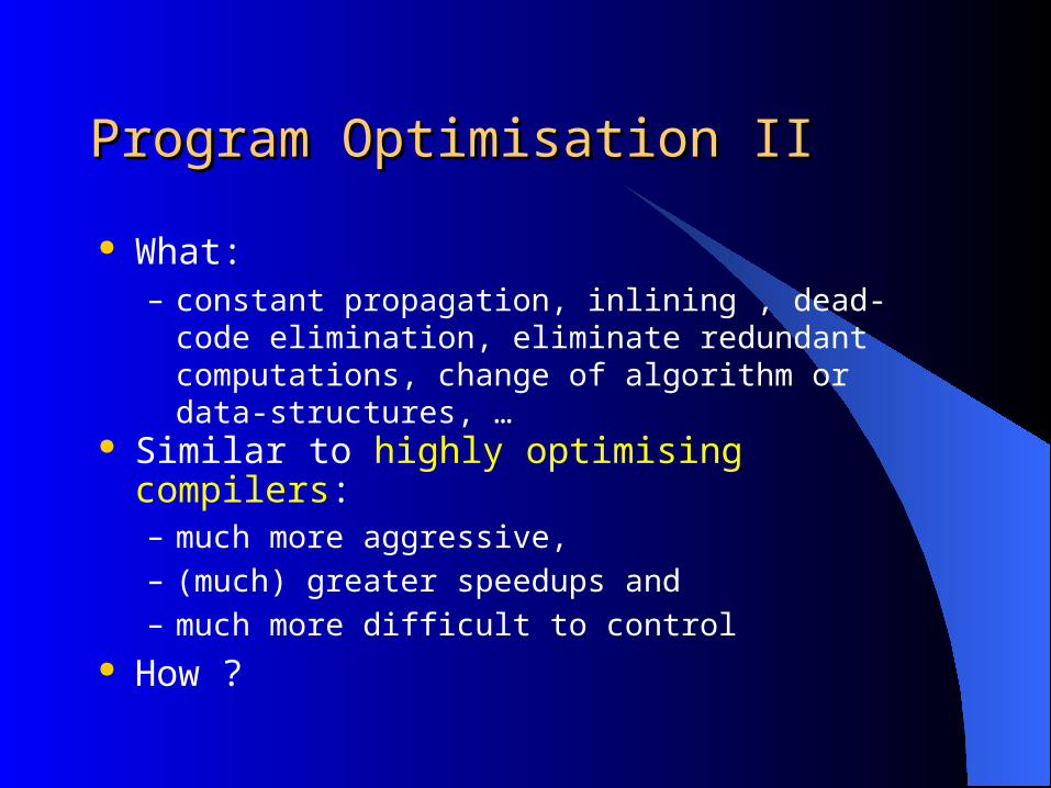
Program Optimisation IIProgram Optimisation II
What:– constant propagation, inlining , dead-code
elimination, eliminate redundant computations, change of algorithm or data-structures, …
Similar to highly optimising compilers: – much more aggressive,– (much) greater speedups and– much more difficult to control
How ?
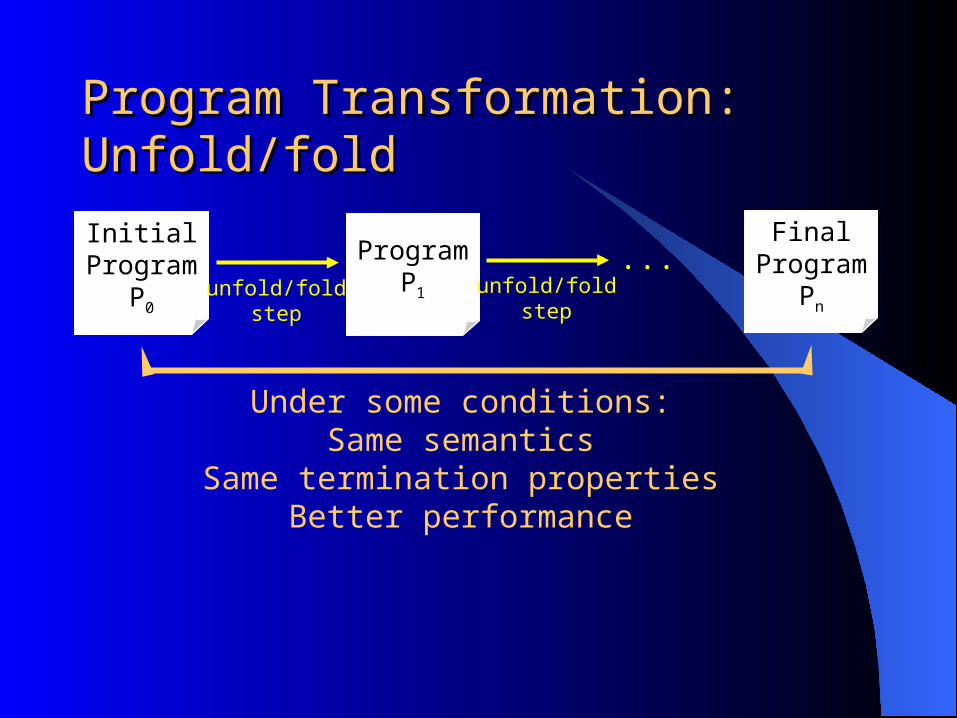
Program Transformation: Unfold/foldProgram Transformation: Unfold/fold
InitialProgram
P0
ProgramP1unfold/fold
step
FinalProgram
Pnunfold/fold
step
...
Under some conditions:Same semantics
Same termination propertiesBetter performance

Program SpecialisationProgram Specialisation
What:– Specialise a program for a
particular application domain How:
– Partial evaluation– Program transformation– Type specialisation– Slicing
DrawingProgram P
P’

OverviewOverview
PartialEvaluationProgram
Specialisation
ProgramTransformation
Program Optimisation

Program AnalysisProgram Analysis
What:– Find out interesting properties of your programs:
Values produced, dependencies, usage, termination, ...
Why:– Verification, debugging
Type checking Check assertions
– Optimisation: Guide compiler (compile time gc, …) Guide source-to-source optimiser

Program Analysis IIProgram Analysis II
How:– Rice’s theorem: all non-trivial properties are
undecidable ! approximations or sufficient conditions
Techniques:– Ad hoc
– Abstract Interpretation [Cousot’77]
– Type Inference
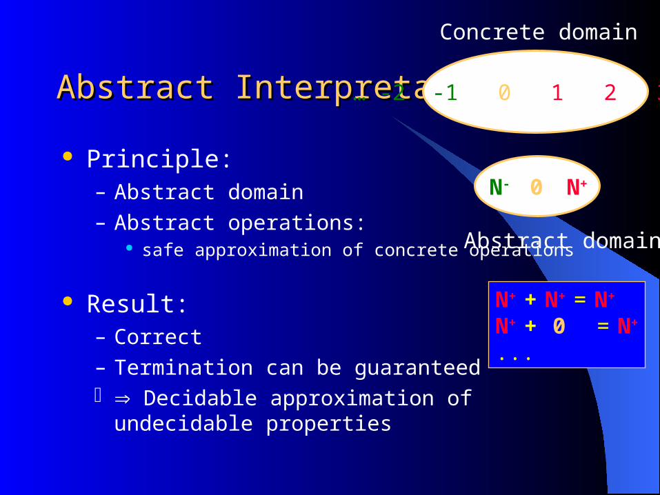
Abstract InterpretationAbstract Interpretation
Principle:– Abstract domain
– Abstract operations: safe approximation of concrete operations
Result:– Correct
– Termination can be guaranteed Decidable approximation of undecidable properties
… -2 -1 0 1 2 3 ...
Concrete domain
N- N+
Abstract domain
0
N+ + N+ = N+
N+ + 0 = N+
...
Part 2:Part 2:
A closer look at partial evaluation: A closer look at partial evaluation: First StepsFirst Steps
1. Overview2. PE: 1st steps3. Why PE4. Issues in PE
A closer look at PE A closer look at PE
Partial Evaluation versus Full Evaluation Why PE Issues in PE: Correctness, Precision, Termination Self-Application and Compilation

2
5
power
Full EvaluationFull Evaluation
Full input Computes full output
2
532power
2
532power
function power(b,e) is if e = 0 then 1 else b*power(b,e-1)
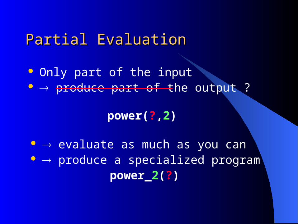
Partial EvaluationPartial Evaluation
Only part of the input produce part of the output ?
power(?,2)
evaluate as much as you can produce a specialized program
power_2(?)

PE: A first attemptPE: A first attempt
Small (functional) language:– constants (N), variables (a,b,c,…)
– arithmetic expressions *,/,+,-, =
– if-then-else, function definitions Basic Operations:
– Evaluate arithmetic operation if all arguments are known
– 2+3 5 5=4 false x+(2+3) x+5
– Replace if-then-else by then-part (resp. else-part) if test-part is known to be true (resp. false)
function power(power(bb,,ee)) is if e = 0 then 1 else b*power(b,e-1)
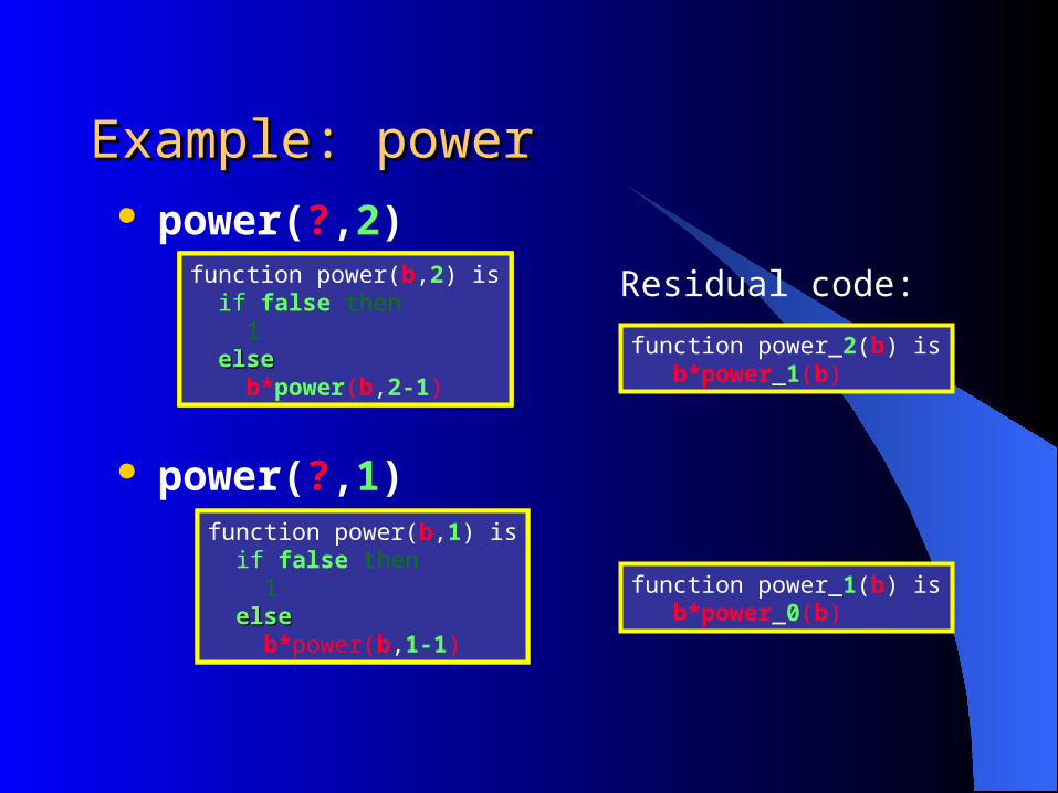
Example: powerExample: power power(?,2)
function power(power(bb,,22)) is if e = 0 then 1 else b*power(b,e-1)
function power(b,2) is ifif 22 = 0= 0 then 1 else b*power(b,e-1)
function power(b,2) is if false then 1 elseelse b*power(b,2-1)
power(?,1)function power(power(bb,,11)) is if e = 0 then 1 else b*power(b,e-1)
function power(b,1) is if false then 1 elseelse b*power(b,1-1)
function power_1(b) is b*power_0(b)
function power_2(b) is b*power_1(b)
Residual code:

Example: power (cont’d)Example: power (cont’d)
power(?,0)
function power(power(bb,,00)) is if e = 0 then 1 else b*power(b,e-1)
function power(b,0) is ifif 00 == 00 then 1 else b*power(b,e-1)
function power(b,0) is if 0 = 0 thenthen 11 else b*power(b,e-1)
function power_0(b) is 11
Residual code:
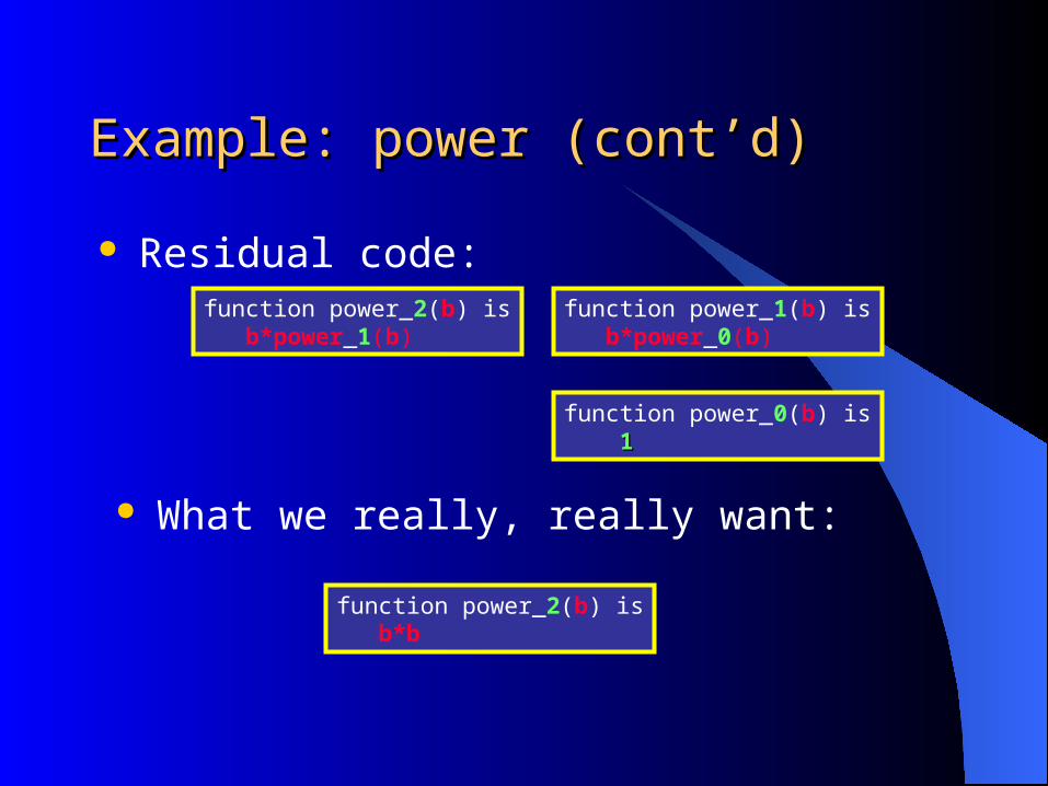
Example: power (cont’d)Example: power (cont’d)
Residual code:
function power_0(b) is 11
function power_1(b) is b*power_0(b)
function power_2(b) is b*power_1(b)
What we really, really want:
function power_2(b) is b*b

Extra Operation: UnfoldingExtra Operation: Unfolding
Replace call by definition
function power(b,2) is if 2 = 0 then 1 elseelse b*power(b,1)
function power(b,2) is if 2 = 0 then 1 elseelse b* (if 1 = 0 then 1 elseelse b*power(b,0))
function power(b,2) is if 2 = 0 then 1 elseelse b* (if 1 = 0 then 1 elseelse b* (if 0 = 0 then 1then 1 else b*power(b,-1)))
function power_2(b) is b*b*1
Residual code:
≈ evaluating thefunction call operation
≈ SQR function
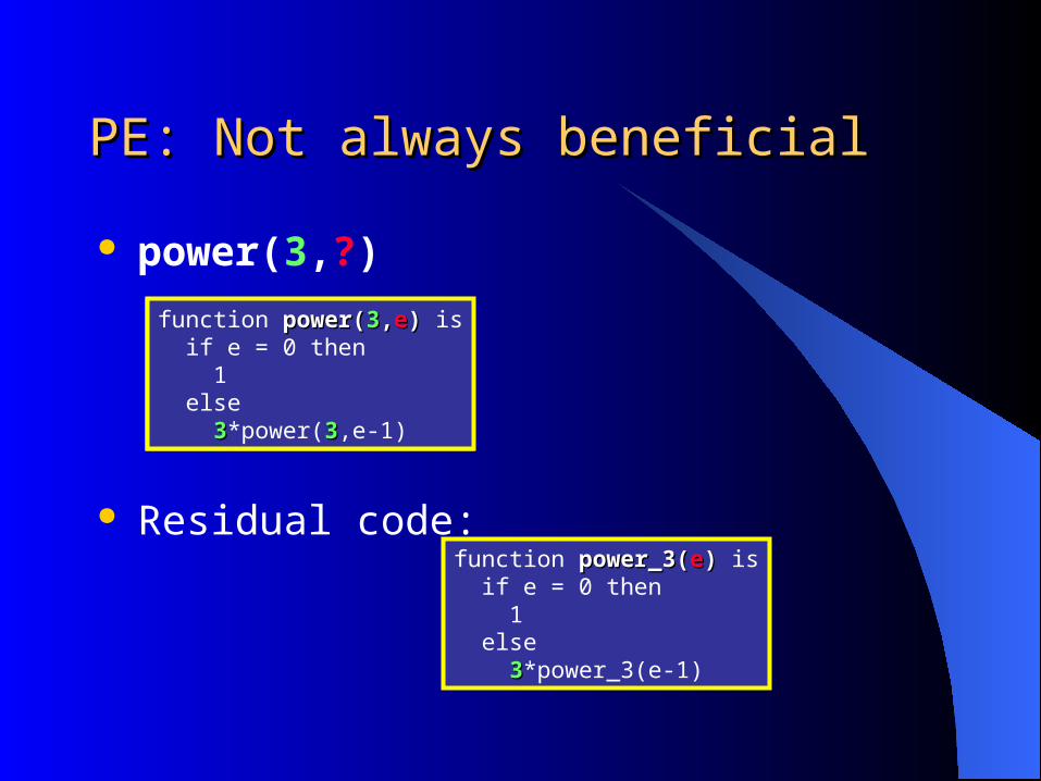
PE: Not always beneficialPE: Not always beneficial
power(3,?)
Residual code:
function power(power(33,,ee)) is if e = 0 then 1 else b*power(b,e-1)
function power(power(33,,ee)) is if e = 0 then 1 else 33*power(33,e-1)
function power_3(power_3(ee)) is if e = 0 then 1 else 33*power_3(e-1)
Part 3:Part 3:
Why Partial Evaluation (and Program Why Partial Evaluation (and Program Optimisation)?Optimisation)?
1. Overview2. PE: 1st steps3. Why PE4. Issues in PE

Constant PropagationConstant Propagation
Static values in programs
function my_program(x) is … y := 2* power(x,33) …
function my_program(x) is … y := 2* x * x * x …
captures inlining and more
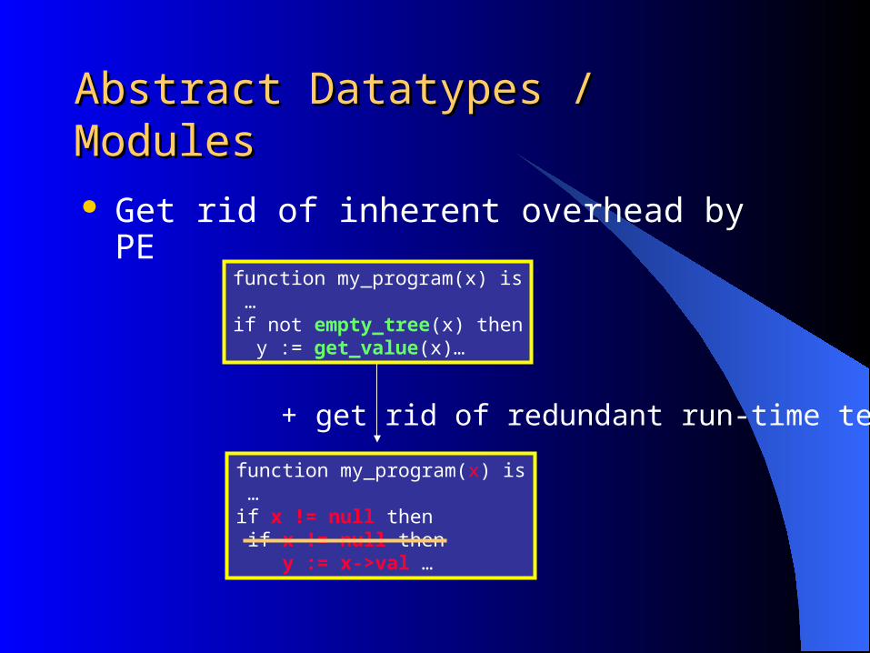
Abstract Datatypes / ModulesAbstract Datatypes / Modules
Get rid of inherent overhead by PE
function my_program(x) is … if not empty_tree(x) then y := get_value(x)…
function my_program(x) is … if x != null then if x != null then y := x->val …
+ get rid of redundant run-time tests
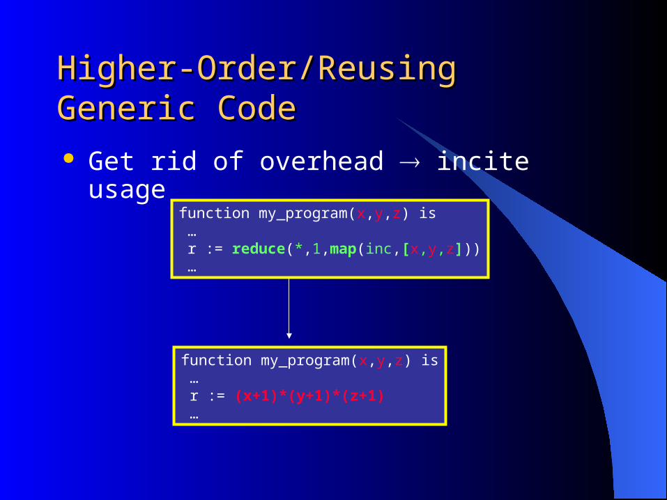
Higher-Order/Reusing Generic CodeHigher-Order/Reusing Generic Code
Get rid of overhead incite usage
function my_program(x,y,z) is … r := reduce(*,1,map(inc,[x,y,z])) …
function my_program(x,y,z) is … r := (x+1)*(y+1)*(z+1) …

Higher-Order IIHigher-Order II
Can generate new functions/procedures
function my_program(x) is … r := reduce(*,1,map(inc,x)) …
function my_program(x) is … r := red_map_1(x) …function red_map_1(x) is if x=nil then return 1 else return x->head* red_map_1(x->tail)

Staged InputStaged Input
Input does not arrive all at once
my_program (x , y , z) … …
5 2 2.1
42

Examples of staged inputExamples of staged input
Ray tracingcalculate_view(Scene,Lights,Viewpoint)
Interpretationinterpreter(ObjectProgram,Call)prove_theorem(FOL-Theory,Theorem)check_integrity(Db_rules,Update)schedule_crews(Rules,Facts)
Speedups– 2: you get your money back– 10: quite typical for interpretation overhead– 100-500 (and even ∞): possible

Ray TracingRay Tracing
Static
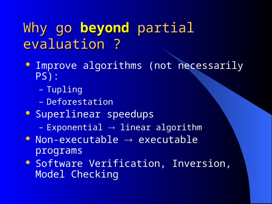
Why go Why go beyondbeyond partial evaluation ? partial evaluation ?
Improve algorithms (not necessarily PS):– Tupling
– Deforestation Superlinear speedups
– Exponential linear algorithm Non-executable executable programs Software Verification, Inversion, Model
Checking

TuplingTuplingCorresponds to
loop-fusion

DeforestationDeforestation

Part 4:Part 4:
Issues in Partial Evaluation and Issues in Partial Evaluation and Program OptimisationProgram Optimisation
Correctness Termination
Efficiency/Precision
Self-application
1. Overview2. PE: 1st steps3. Why PE4. Issues in PE
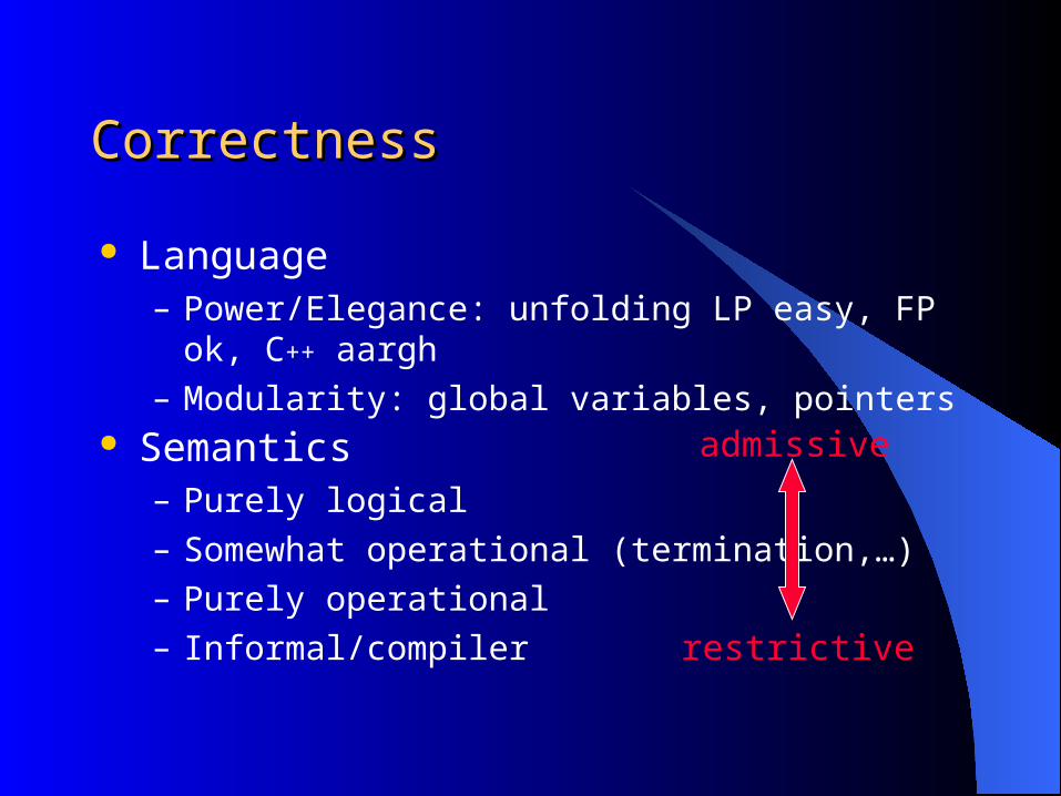
CorrectnessCorrectness
Language– Power/Elegance: unfolding LP easy, FP ok, C++ aargh
– Modularity: global variables, pointers Semantics
– Purely logical
– Somewhat operational (termination,…)
– Purely operational
– Informal/compilerrestrictive
admissive

Programming Language for CourseProgramming Language for Course
Lectures use mainly LP and FP– Don’t distract from essential issues
– Nice programming paradigm
– A lot of room for speedups
– Techniques can be useful for other languages, but Correctness will be more difficult to establish Extra analyses might be required (aliasing, flow analysis, …)

Efficiency/PrecisionEfficiency/Precision
Unfold enough but not too much– Enough to propagate partial information
– But still ensure termination
– Binding-time Analysis (for offline systems): Which expressions will be definitely known Which statements can be executed
Allow enough polyvariance but not too much– Code explosion problem
– Characteristic trees
x := 2+y;p(x)
y=5 p(7)
p(7) p(9) p(11) p(13) ...

TerminationTermination
Who cares PE should terminate when the program does PE should always terminate " within reasonable time bounds
State of the art

Self-ApplicationSelf-Application
Principle:– Write a partial evaluator (program specialiser,…)
which can specialise itself Why:
– Ensures non-trivial partial evaluator
– Ensures non-trivial language
– Optimise specialisation process
– Automatic compiler generation !

Compiling by PECompiling by PE
InterpreterObject Program P
Call1Call2
Call3
Result1Result2
Result3
PE
P-Interpreter
Call1Call2
Call3
Result1Result2
Result3

Compiler Generation by PECompiler Generation by PE
Interpreter IObject Program P
PE
P-Interpreter
Object Program Q
Q-Interpreter
Object Program R
R-Interpreter
static
PE’ I-PE
Object Program PObject Program QObject Program R
= Compiler !
Useful for:Lge Extensions,Debugging,DSL,...

Cogen Generation by PECogen Generation by PE
PEInterpreter P
PE’
P-Compiler
Interpreter Q
Q-Compiler
Interpreter R
R-Compiler
static
PE’’ PE-PE
Interpreter PInterpreter QInterpreter R
= Compiler Generator !
3rd FutamuraProjection

Part 5:Part 5:
Overview of the course (remainder)Overview of the course (remainder)

Overview of the Course: Lecture 2Overview of the Course: Lecture 2
Partial Evaluation of Logic Programs:First Steps– Topics
A short (re-)introduction to Logic Programming How to do partial evaluation of logic programs
(called partial deduction): first steps
– Outcome: Enough knowledge of LP to follow the rest Concrete idea of PE for one particular language

Overview of the Course: Lecture 3Overview of the Course: Lecture 3
(Online) Partial Deduction: Foundations, Algorithms and Experiments– Topics
Correctness criterion and results Control Issues: Local vs. Global; Online vs. Offline Local control solutions: Termination Global control: Ch. trees, WQO's at the global level Relevance for other languages and applications Full demo of Ecce system
– Outcome: How to control program specialisers (analysers, ...) How to prove them correct

Overview of the Course: Lecture 4(?)Overview of the Course: Lecture 4(?)
Extending Partial Deduction:– Topics
Unfold/Fold vs PD Going from PD to Conjunctive PD Control issues, Demo of Ecce Abstract Interpretation vs Conj. PD (and Unfold/Fold) Integrating Abstract Interpretation Applications (+ Demo): Infinite Model Checking
– Outcome How to do very advanced/fancy optimisations

Overview of the Course:Overview of the Course:Other LecturesOther Lectures By Morten Heine Sørensen
Context:– Functional Programming Languages
Topics:– Supercompilation
– Unfold/fold
– ...
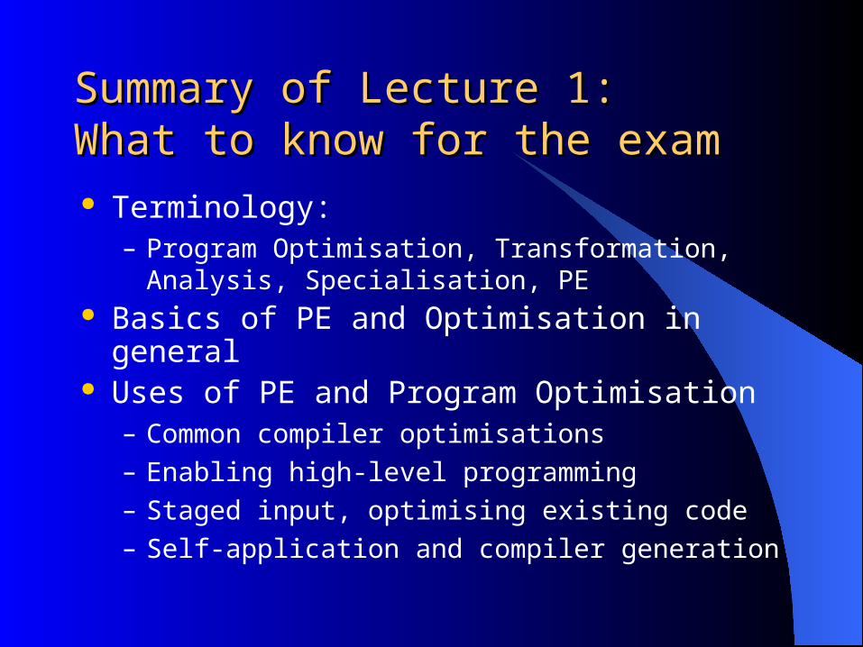
Summary of Lecture 1:Summary of Lecture 1:What to know for the examWhat to know for the exam Terminology:
– Program Optimisation, Transformation, Analysis, Specialisation, PE
Basics of PE and Optimisation in general Uses of PE and Program Optimisation
– Common compiler optimisations
– Enabling high-level programming
– Staged input, optimising existing code
– Self-application and compiler generation

04/19/23
Optimisation of Declarative Programs Optimisation of Declarative Programs
Lecture 2Lecture 2
Michael Leuschel
Declarative Systems & Software EngineeringDept. Electronics & Computer ScienceUniversity of Southampton
http:// www.ecs.soton.ac.uk/~mal

Overview of Lecture 2:Overview of Lecture 2:
Recap of LP First steps in PE of LP
– Why is PE non-trivial ?
– Generating Code: Resultants
– Correctness Independence, Non-triviality, Closedness Results
– Filtering
– Small demo of the ecce system
1. LP Refresher2. PE of LP: 1st steps

Part 1:Part 1:Brief Refresher onBrief Refresher onLogic Programming and PrologLogic Programming and Prolog
1. LP Refresher2. PE of LP: 1st steps

Brief History of Logic ProgrammingBrief History of Logic Programming
Invented in 1972– Colmerauer (implementation,
Prolog = PROgrammation en LOGique)
– Kowalski (theory) Insight: subset of First-Order Logic
– efficient, procedural interpretation based on resolution (Robinson 1965 + Herbrand 1931)
– Program = theory
– Computation = logical inference

Features of Logic ProgrammingFeatures of Logic Programming
Declarative Language– State what is to be computed, not how
Uniform Language to express and reason about– Programs, specifications
– Databases, queries,… Simple, clear semantics
– Reasoning about correctness is possible
– Enable powerful optimisations
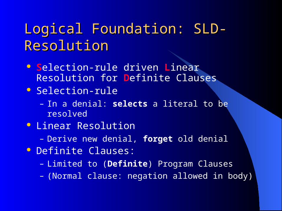
Logical Foundation: SLD-ResolutionLogical Foundation: SLD-Resolution
Selection-rule driven Linear Resolution for Definite Clauses
Selection-rule– In a denial: selects a literal to be resolved
Linear Resolution– Derive new denial, forget old denial
Definite Clauses:– Limited to (Definite) Program Clauses
– (Normal clause: negation allowed in body)
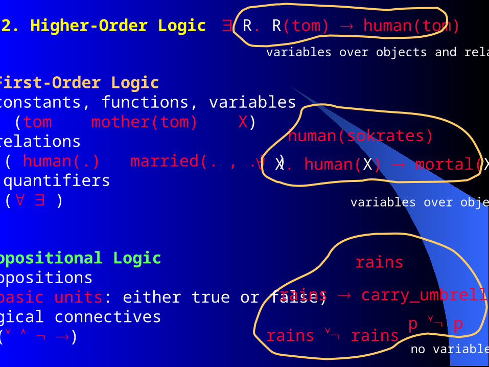
0. Propositional Logic - propositions (basic units: either true or false) - logical connectives ( )
1. First-Order Logic - constants, functions, variables (tom mother(tom) X) - relations ( human(.) married(. , .) ) - quantifiers ( )
p prains rains
rains carry_umbrella
2. Higher-Order Logic
X. human(X) mortal(X)
human(sokrates)
rains
R. R(tom) human(tom)
no variables
variables over objects and relations
variables over objects
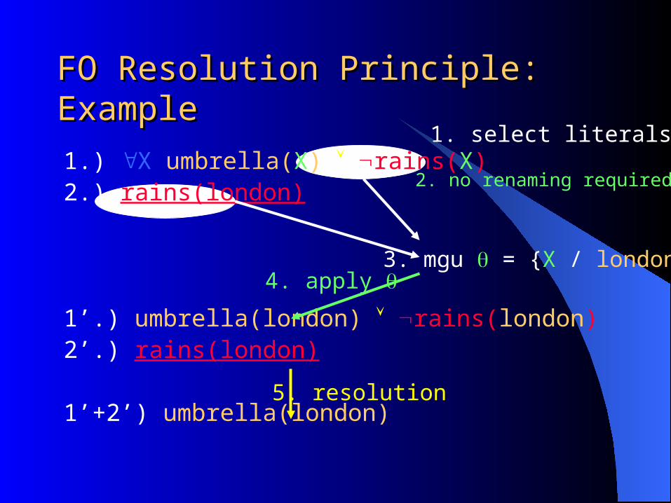
FO Resolution Principle: ExampleFO Resolution Principle: Example
1.) X umbrella(X) rains(X)2.) rains(london)
1’.) umbrella(london) rains(london)2’.) rains(london)
1’+2’) umbrella(london)
3. mgu = {X / london}
5. resolution
4. apply
1. select literals
2. no renaming required

TerminologyTerminology
SLD-Derivation for P { G}– Sequence of goals and mgu’s, at every step:
Apply selection rule on current goal (very first goal: G) Unify selected literal with the head of a program clause Derive the next goal by resolution
SLD-Refutation for P { G}– SLD-Derivation ending in
Computed answer for P { G}– Composition of mgu’s of a SLD-refutation, restricted
to variables in G

SLD DerivationSLD Derivation
1) knows_logic(X) good_student(X) teacher(Y,X) logician(Y)
2) good_student(tom)3) logician(peter)4) teacher(peter,tom)
knows_logic(Z)
good_student(X) teacher(Y,X) logician(Y)
teacher(Y,tom) logician(Y)
logician(peter)
Computed answer = {Z/tom}
P J knows_logic(tom) ??
{Z/X}
{X/tom}
{Y/peter}
{}
G

BacktrackingBacktracking
1) knows_logic(X) good_student(X) teacher(Y,X) logician(Y)
2) good_student(jane)3) good_student(tom)4) logician(peter)5) teacher(peter,tom)
knows_logic(Z)
good_student(X) teacher(Y,X) logician(Y)
teacher(Y,jane) logician(Y)
teacher(Y,tom) logician(Y)
logician(peter)
Backtracking required !
Try to resolve with another clause

SLD-TreesSLD-Trees knows_logic(Z)
good_student(X) teacher(Y,X) logician(Y)
teacher(Y,tom) logician(Y)
logician(peter)
teacher(Y,jane) logician(Y)
Prolog: explores this tree Depth-First, always selects leftmost literal
fail
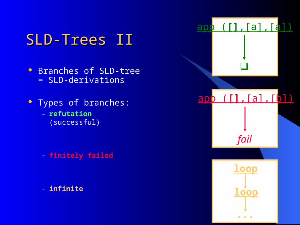
SLD-Trees IISLD-Trees II
Branches of SLD-tree = SLD-derivations
Types of branches:– refutation (successful)
– finitely failed
– infinite
app ([],[a],[a])
app ([],[a],[b])
fail
loop
loop
...
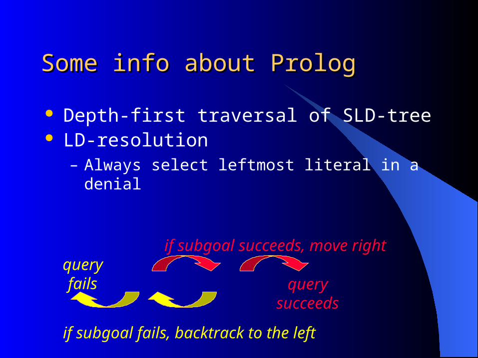
Some info about PrologSome info about Prolog
Depth-first traversal of SLD-tree LD-resolution
– Always select leftmost literal in a denial
querysucceeds
if subgoal succeeds, move right
if subgoal fails, backtrack to the left
queryfails
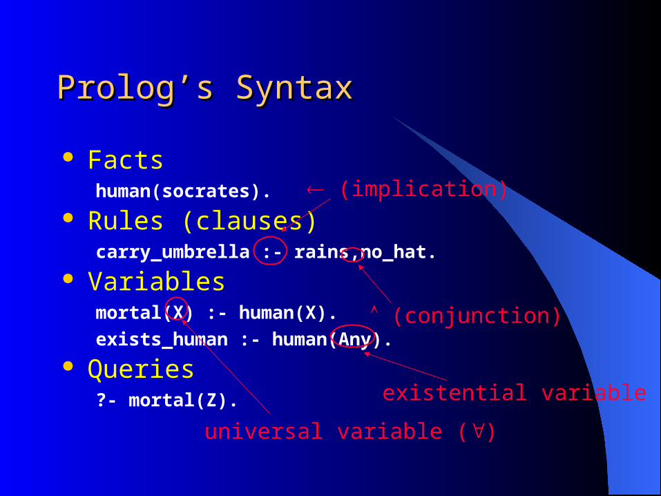
Prolog’s SyntaxProlog’s Syntax
Factshuman(socrates).
Rules (clauses)carry_umbrella :- rains,no_hat.
Variablesmortal(X) :- human(X).
exists_human :- human(Any). Queries
?- mortal(Z).
(implication)
(conjunction)
existential variable ()
universal variable ()

Prolog’s DatastructuresProlog’s Datastructures
Constants:human(socrates).
Integers, Reals:fib(0,1).
pi(3.141). (Compound) Terms:
head_of_list(cons(X,T),X).
tail_of_list(cons(X,T),T).
?- head_of_list(cons(1,cons(2,nil)),R).
functor
lower-case
Prolog actually uses . (dot) for lists

Lists in PrologLists in Prolog
Empty list:– [] (syntactic sugar for nil )
Non-Empty list with first element H and tail T:– [H|T] (syntactic sugar for .(H,T) )
Fixed-length list:– [a] (syntactic sugar for [a | [] ] = .(a,nil) )
– [a,b,c] (syntactic sugar for [a | [b | [c | [] ] ] ] )

Part 2:Part 2:
Partial Evaluation of Logic Programs:Partial Evaluation of Logic Programs:First StepsFirst Steps
1. LP Refresher2. PE of LP: 1st steps

What is Full Evaluation in LPWhat is Full Evaluation in LP
In our context: full evaluation =constructing complete SLD-tree for a goal every branch either
successful, failed or infinite
SLD can handle variables !! can handle partial data-structures
(not the case for imperative or functional programming)
Unfolding = ordinary SLD-resolution !
Partial evaluation = full evaluation ??
Partial evaluation trivial ??

ExampleExampleapp([],L,L).app([H|X],Y,[H|Z]) :- app(X,Y,Z).
app ([a],B,C)
app ([],B,C’)
{C/[a|C’]}
{C’/B}
app([a],B,[a|B]).
app_a(B,[a|B]).
Apply c.a.s. oninitial goal
(+ filter out static part)

Example:Example:RuntimeRuntimeQueryQuery
app([],L,L).app([H|X],Y,[H|Z]) :- app(X,Y,Z).
app ([a],[b],C)
{C/[a,b]}
app([a],B,[a|B]).
app_a(B,[a|B]).
app ([a],[b],C)
app ([],[b],C’)
{C/[a|C’]}
{C’/[b]}app_a ([b],C)
{C/[a,b]}
c.a.s.: {C/[a,b]}
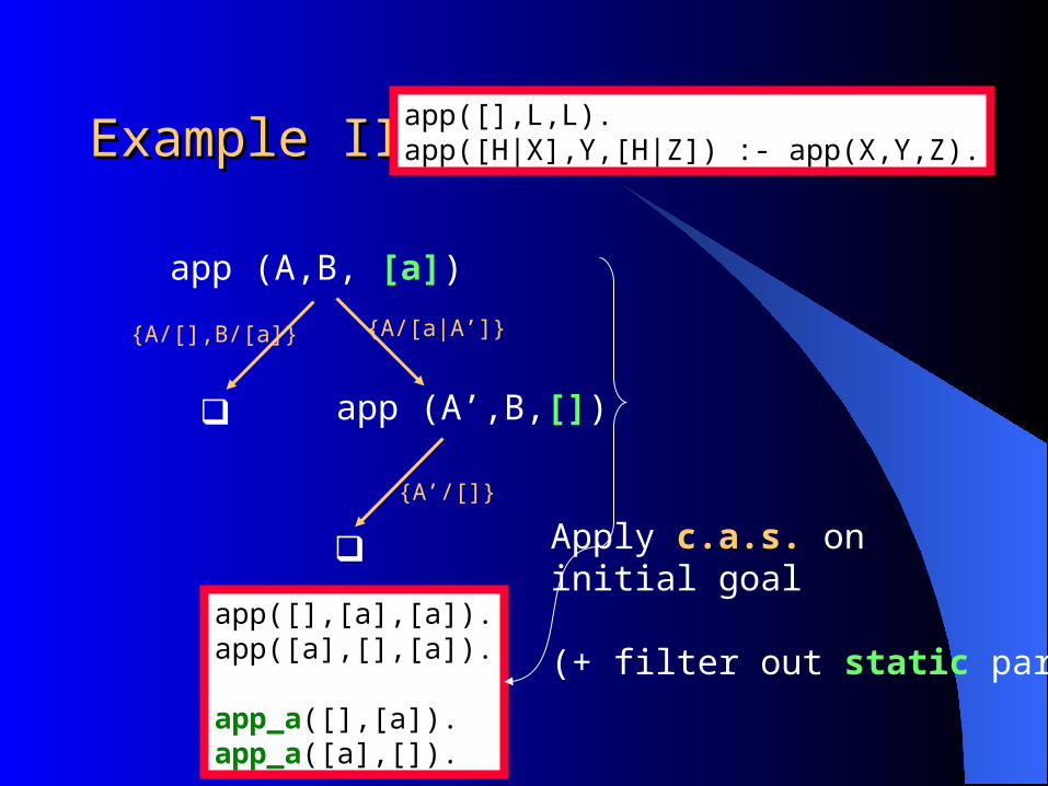
Example IIExample IIapp([],L,L).app([H|X],Y,[H|Z]) :- app(X,Y,Z).
app (A,B, [a])
app (A’,B,[])
{A/[a|A’]}
{A/[],B/[a]}
app([],[a],[a]).app([a],[],[a]).
app_a([],[a]).app_a([a],[]).
Apply c.a.s. oninitial goal
(+ filter out static part)
{A’/[]}
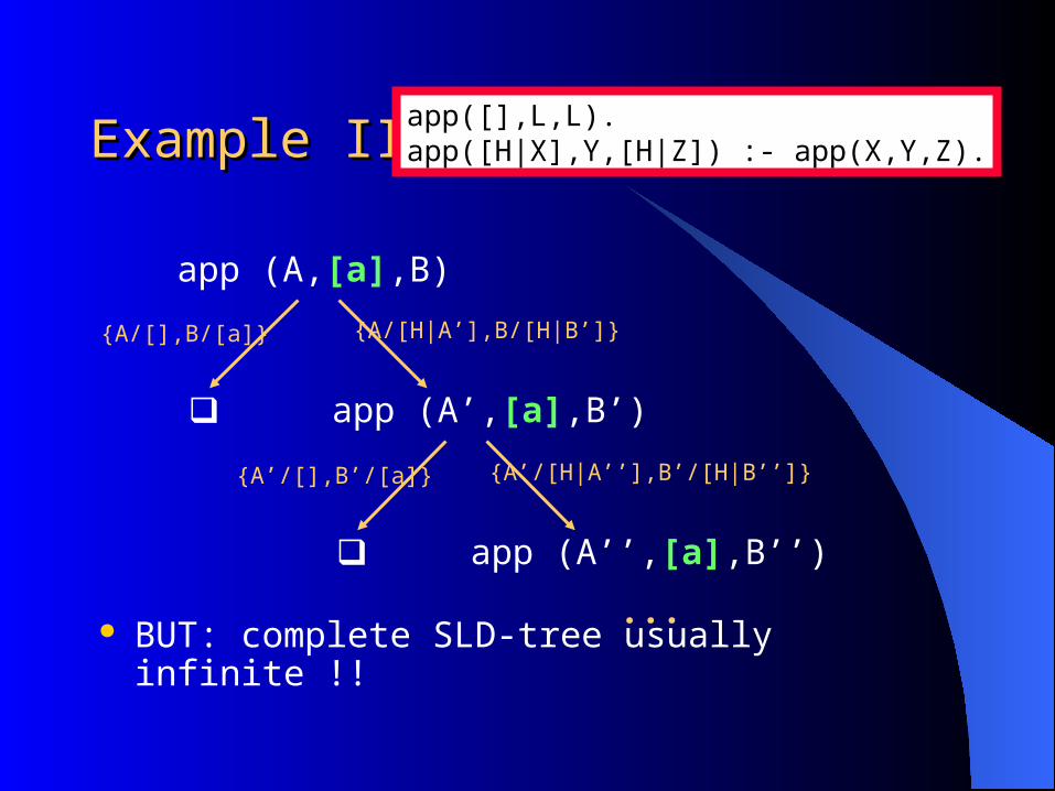
Example IIIExample III
BUT: complete SLD-tree usually infinite !!
app([],L,L).app([H|X],Y,[H|Z]) :- app(X,Y,Z).
app (A,[a],B)
app (A’,[a],B’)
{A/[],B/[a]} {A/[H|A’],B/[H|B’]}
app (A’’,[a],B’’)
{A’/[],B’/[a]} {A’/[H|A’’],B’/[H|B’’]}
...

Partial DeductionPartial Deduction
Basic Principle:– Instead of building one complete SLD-tree:
Build a finite number of finite “SLD- trees” !
– SLD-trees can be incomplete 4 types of derivations in SLD-trees:
– Successful, failed, infinite
– Incomplete: no literal selected

Example (revisited)Example (revisited)
app([],L,L).app([H|X],Y,[H|Z]) :- app(X,Y,Z).
app (A,[a],B)
app (A’,[a],B’)
{A/[],B/[a]} {A/[H|A’],B/[H|B’]}
app_a([],[a]).app_a([H|A’],[H|B’]) :- app_a(A’,B’).
STOP
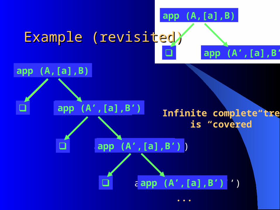
Example (revisited)Example (revisited)
app (A,[a],B)
app (A’,[a],B’)
app (A’’,[a],B’’)
...
app (A’’’,[a],B’’’)
app (A,[a],B)
app (A’,[a],B’)
app (A,[a],B)
app (A’,[a],B’)
app (A,[a],B)
app (A’,[a],B’)
app (A,[a],B)
app (A’,[a],B’) Infinite complete treeis “covered”

Main issues in PD (& PE in general)Main issues in PD (& PE in general)
How to construct the specialised code ? When to stop unfolding (building SLD-tree) ? Construct SLD-trees for which goals ? When is the result correct ?
Will be addressed in this Lecture !

Generating Code:Generating Code:ResultantsResultants Resultant of
SLD-derivation
is the formula: G01...k Gk
if n=1: Horn clause !
A1,…,Ai,…,An
G1
G2
...
Gk
0
1
k
G0

Resultants: ExampleResultants: Example
app([],L,L).app([H|X],Y,[H|Z]) :- app(X,Y,Z).
app (A,[a],B)
app (A’,[a],B’)
{A/[],B/[a]} {A/[H|A’],B/[H|B’]}
app([],[a],[a]).app([H|A’],[a],[H|B’]) :- app(A’,[a],B’).
STOP

Formalisation of Partial DeductionFormalisation of Partial Deduction
Given a set S = {A1,…,An} of atoms: Build finite, incomplete SLD-trees for each Ai
For every non-failing branch:– generate 1 specialised clause by
computing the resultants
When is this correct ?

Correctness 1: Non-trivial treesCorrectness 1: Non-trivial trees
Trivial tree:
Resultant:app (A,[a],B) app (A,[a],B)
loops!
Correctness condition:Perform at least one derivation step
app (A,[a],B)
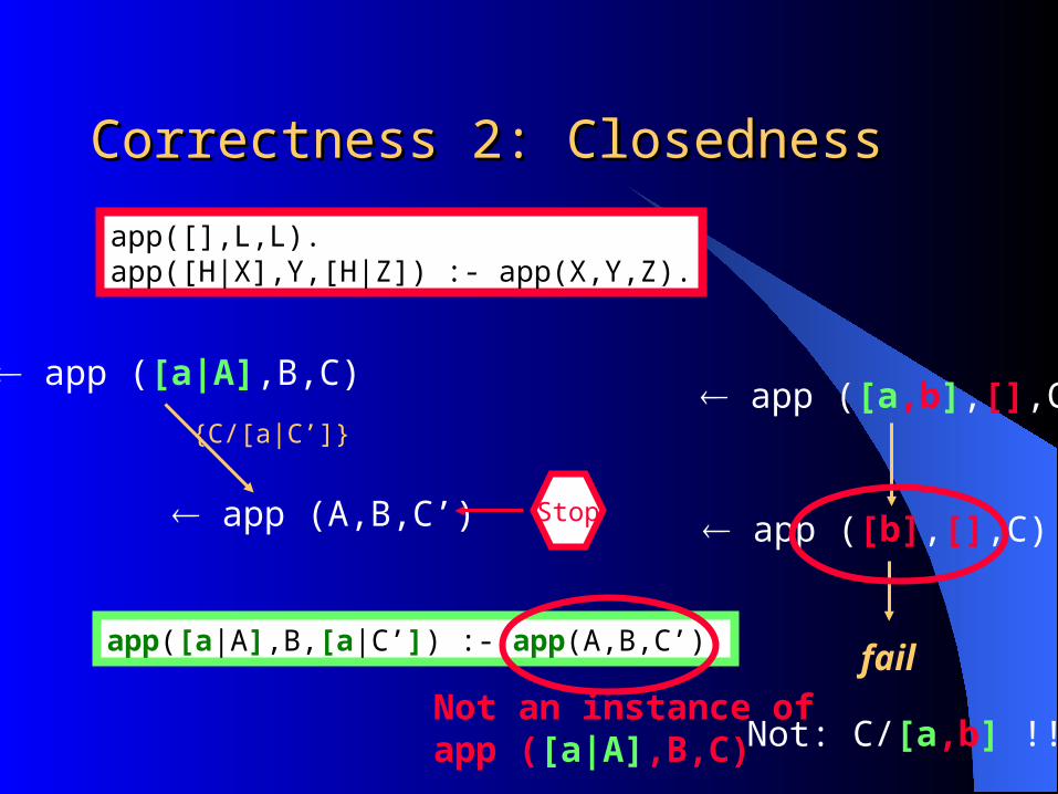
Correctness 2: ClosednessCorrectness 2: Closedness
app([],L,L).app([H|X],Y,[H|Z]) :- app(X,Y,Z).
app ([a|A],B,C)
app (A,B,C’)
{C/[a|C’]}
app([a|A],B,[a|C’]) :- app(A,B,C’).
Stop
app ([a,b],[],C)
app ([b],[],C)
fail
Not: C/[a,b] !!Not an instance ofapp ([a|A],B,C)

Closedness ConditionClosedness Condition
To avoid uncovered calls at runtime:
All predicate calls– in the bodies of specialised clauses
(= atoms in leaves of SLD-trees !)
– in the calls to the specialised program must be instances of at least one of the atoms in
S = {A1,…,An}

Correctness 3: IndependenceCorrectness 3: Independence
app([],L,L).app([H|X],Y,[H|Z]) :- app(X,Y,Z).
app ([a|A],B,C)
app (A,B,C’)
{C/[a|C’]}
app([a|A],B,[a|C’]) :- app(A,B,C’).
app([],C,C).app([H|A’],B,[H|C’]) :- app(A’,B,C’).
app (A,B,C)
app (A’,B,C’)
{A/[],B/C} {A/[H|A’],C/[H|C’]}
Closedness:Ok

Extra answersExtra answers
app ([],Y,Z’)
app([a|A],B,[a|C’]) :- app(A,B,C’).
app([],C,C).app([H|A’],B,[H|C’]) :- app(A’,B,C’).
app ([X],Y,Z)
app ([],Y,Z’)
{X/a,Z/[a|Z’]}
X = a, Z=[a|Y]
{Z/[X|Z’]}
Z=[X|Y]
Extra answer !+
more instantiated !!

Independence ConditionIndependence Condition
To avoid extra and/or more instantiated answers: require that no two atoms in S = {A1,…,An} have
a common instance
S = {app ([a|A],B,C), app(A,B,C)}– common instances = app([a],X,Y), app([a,b],[],X), …
How to ensure independence ?– Just Renaming !

Renaming: No Extra answersRenaming: No Extra answers
app([a|A],B,[a|C’]) :- app(A,B,C’).
app([],C,C).app([H|A’],B,[H|C’]) :- app(A’,B,C’).
app ([X],Y,Z)
app ([],Y,Z’) app ([],Y,Z’)
{X/a,Z/[a|Z’]}
X = a, Z=[a|Y]
{Z/[X|Z’]}
Z=[X|Y]
app_a([a|A],B,[a|C’]) :- app(A,B,C’).
app([],C,C).app([H|A’],B,[H|C’]) :- app(A’,B,C’).
No extra answer !

Soundness & CompletenessSoundness & Completeness
P’ obtained by partial deduction from P
If non-triviality, closedness, independence conditions are satisfied:
P’ {G} has an SLD-refutation with c.a.s. iff P {G}has
P’ {G} has a finitely failed SLD-tree iffP {G}has
Lloyd, Shepherdson: J. Logic Progr. 1991

A more detailed exampleA more detailed example
map(P,[],[]).map(P,[H|T],[PH|PT]) :- C=..[P,H,PH], call(C),map(P,T,PT).inv(0,1).inv(1,0).
map (inv,L,R)
{L/[],R/[]}
C=..[inv,H,PH], call(C),map(inv,L’,R’)
{L/[H|L’],R/[PH|R’]}
inv(H,PH),map(inv,L’,R’)
call(inv(H,PH)),map(inv,L’,R’)
{C/inv(H,PH)}
map(inv,[],[]).map(inv,[0|L’],[1|R’]) :- map(inv,L’,R’).map(inv,[1|L’],[0|R’]) :- map(inv,L’,R’). map(inv,L’,R’)
{H/0,PH/1}
map(inv,L’,R’)
{H/1,PH/0}
map(P,[],[]).map(P,[H|T],[PH|PT]) :- C=..[P,H,PH], call(C),map(P,T,PT).inv(0,1).inv(1,0).
Overhead removed: 2 faster

FilteringFiltering
map(P,[],[]).map(P,[H|T],[PH|PT]) :- C=..[P,H,PH], call(C),map(P,T,PT).inv(0,1).inv(1,0).
map (inv,L,R)
{L/[],R/[]}
C=..[inv,H,PH], call(C),map(inv,L’,R’)
{L/[H|L’],R/[H|R’]}
inv(H,PH),map(inv,L’,R’)
call(inv(H,PH)),map(inv,L’,R’)
{C/inv(H,PH)}
map(inv,[],[]).map(inv,[0|L’],[1|R’]) :- map(inv,L’,R’).map(inv,[1|L’],[0|R’]) :- map(inv,L’,R’).
map(inv,L’,R’)
{H/0,PH/1}
map(inv,L’,R’)
{H/1,PH/0}
map_1(L,R)
map_1([],[]).map_1([0|L’],[1|R’]) :- map_1(L’,R’).map_1([1|L’],[0|R’]) :- map_1(L’,R’).

Renaming+Filtering: CorrectnessRenaming+Filtering: Correctness
Correctness results carry over– Benkerimi,Hill J. Logic & Comp 3(5), 1993
No worry about Independence
Non-triviality also easy to ensure only worry that remains (for correctness):
Closedness

Small Demo (ecce system)Small Demo (ecce system)
Append Higher-Order Match Interpreter

Summary of part 2Summary of part 2
Partial evaluation in LP Generating Code:
– Resultants, Renaming, Filtering Correctness conditions:
– non-triviality
– closedness
– independence Soundness & Completeness
04/19/23
Optimisation of Declarative Programs Optimisation of Declarative Programs
Lecture 3Lecture 3
Michael Leuschel
Declarative Systems & Software EngineeringDept. Electronics & Computer ScienceUniversity of Southampton
http:// www.ecs.soton.ac.uk/~mal
Part 1:Part 1:Controlling Partial Deduction:Controlling Partial Deduction:LocalLocal Control & Control & TerminationTermination
1. Local Control & Termination2. Global Control & Abstraction
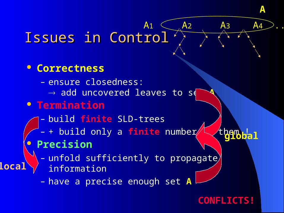
Issues in ControlIssues in Control
Correctness– ensure closedness:
add uncovered leaves to set A Termination
– build finite SLD-trees
– + build only a finite number of them ! Precision
– unfold sufficiently to propagate information
– have a precise enough set A
global
local
A1 A2 A3 A4 ...
A
CONFLICTS!
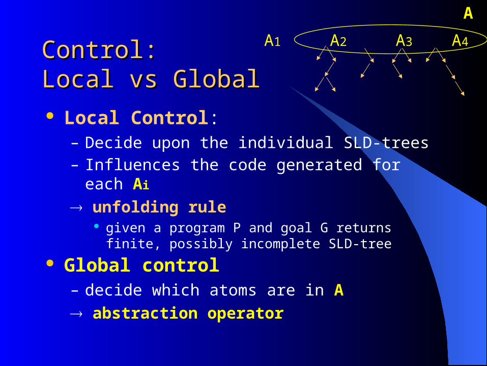
Control:Control:Local vs GlobalLocal vs Global Local Control:
– Decide upon the individual SLD-trees– Influences the code generated for each Ai
unfolding rule given a program P and goal G returns finite, possibly
incomplete SLD-tree
Global control– decide which atoms are in A
abstraction operator
A1 A2 A3 A4 ...
A

Generic AlgorithmGeneric Algorithm
Input: program P and goal GOutput: specialised program P’Initialise: i=0, A0 = atoms in G
repeat Ai+1 := Ai
for each a Ai do Ai+1 := Ai+1 leaves(unfold(a)) end for Ai+1 := abstract(Ai+1) until Ai+1 = Ai
compute P’ via resultants+renaming

Overview Lecture 3Overview Lecture 3
Local Control– Determinacy
– Ensuring Termination Wfo’s, Wqo’s
Global Control– abstraction
– most specific generalisation
– characteristic trees

(Local) Termination(Local) Termination
Who cares PE should terminate when the program does PE should always terminate " within reasonable time bounds
State of the art
Well-founded ordersWell-quasi orders

Determinate UnfoldingDeterminate Unfolding
Unfold atoms which match only 1 clause(only exception: first unfolding step)– avoids code explosion
– no duplication of work
– good heuristic for pre-computing
– too conservative on its own
– termination always ? No when program terminates ??

DuplicationDuplicationapp([],L,L).app([H|X],Y,[H|Z]) :- app(X,Y,Z).
app(A,B,C),app (_I,C,[a,a])
app(A,B,C),app (_I,C,[a])app(A,B,[a,a])
app(A,B,C),app (_I,C,[])app(A,B,[a])
app(A,B,[])
a2(A,B,[a,a]) :- app(A,B,[a,a]).a2(A,B,[a]) :- app(A,B,[a]).a2(A,B,[]) :- app(A,B,[]).

Duplication 2Duplication 2
Solutions:– Determinacy!
– Follow runtime selection rule
a2(A,B,[a,a]) :- app(A,B,[a,a]).a2(A,B,[a]) :- app(A,B,[a]).a2(A,B,[]) :- app(A,B,[]).
a2([a],[],C)
app [a],[],[a]) app [a],[],[])app([a],[],[a,a])
app([],[],[a])
fail

Order of SolutionsOrder of Solutions
t(A,B) :- p(A,C),p(C,B).p(a,b).p(b,a).
p(A,B),p(B,C)
p(A,b)p(A,a)
t(b,b).t(a,a).
t(A,C) Same solutions:– Determinacy!
– Follow runtime selection rule

LookaheadLookahead
Also unfold ifatom matches more than 1 clause
+ only 1 clause remains after further unfolding
– less conservative
– still ensures no duplication, explosion
fail

Lookahead exampleLookahead example
sel (4,[5],R)
{}
4<5, sel(4,[],R’)
{R/[5|R’]}
s4([5],[5]).
sel(P,[],[]).sel(P,[H|T],[H|PT]) :- P<H, sel(P,T,PT).sel(P,[H|T],PT) :- P>=H, sel(P,T,PT).s4(L,PL) :- sel(4,L,PL).
4>=5, sel(4,[],R)
{R/[]}
sel(4,[],R’)fail
s4([5],R)

ExampleExampleapp([],L,L).app([H|X],Y,[H|Z]) :- app(X,Y,Z).
app (A,[a],A)
app (A’,[a],A’)
{A/[H|A’]}
Unificationfails
app (A’’,[a],A’’)
{A’/[H|A’’]}
Unificationfails
app (A’’’,[a],A’’’)
{A’’/[H|A’’’]}
Unificationfails
At runtime:app([],[a],[]) terminates !!!
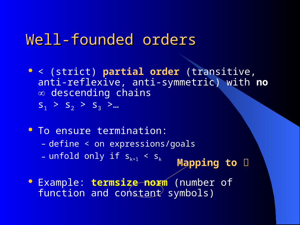
Well-founded ordersWell-founded orders
< (strict) partial order (transitive, anti-reflexive, anti-symmetric) with no descending chainss1 > s2 > s3 >…
To ensure termination:– define < on expressions/goals
– unfold only if sk+1 < sk
Example: termsize norm (number of function and constant symbols)
Mapping to

ExampleExampleapp([],L,L).app([H|X],Y,[H|Z]) :- app(X,Y,Z).
app ([a,b|C],A,B)
app ([b|C],A,B’)
{B/[a|A’]}
Unificationfails
app (C,A,B’’)
{B’/[b|A’’]}
Unificationfails Stop
app (C’,A,B’’’)
{C/[H|C’],B’’/[H|A’’’]}
|.| = 3
|.| = 5
|.| = 1
|.| = 1|.| = 0
Ok
Ok

Other wfo’sOther wfo’s
linear norms, semi-linear norms– |f(t1,…,tn)| = cf + cf,1 |t1| + … + cf,n |tn|
– |X| = cV
lexicographic ordering– |.|1, …, |.|k : first use |.|1, if equal use |.|2...
multiset ordering– {t1,…,tn} < {s1,…,sk, t2,…,tn} if all si < t1
recursive path ordering ...

More general-than/Instance-ofMore general-than/Instance-of
A>B if A strictly more general than B
p(X) p(s(X)) p(s(s(X))) …
not a wfo
A>B if A strict instance of B
p(s(s(X))) p(s(X)) p(X) X
is a wfo (Huet’80)

Refining wfo’sRefining wfo’srev([],L,L).rev([H|X],A,R) :- rev(X,[H|A],R).
rev ([a,b|C],[],R)
rev ([b|C],[a],R)Unificationfails
rev (C,[b,a],R)Unificationfails Stop
rev (C’,[H,b,a],R)
{C/[H|C’]}
|.| = 6
|.| = 6
measure just arg 1
Ok
|.| = 4
|.| = 2
|.| = 0
|.| = 0

Well-quasi ordersWell-quasi orders
quasi order (reflexive and transitive) withevery infinite sequence s1,s2,s3,… we can findi<j such that si sj
To ensure termination:– define on expressions/goals
– unfold only if for no i<k+1: si sk+1

Alternative Definitions of wqo’sAlternative Definitions of wqo’s
All quasi orders ’ which contain (ab a’b) are wfo’s – can be used to generate wfo’s
Every set has a finite generating set (ab a generates b)
For every infinite sequence s1,s2,… we can find an infinite subsequence r1,r2,… such that ri ri+1
Wfo with finitely many incomparable elements ...

Examples of wqo’sExamples of wqo’s
AB if A and B have same top-level functor
– p(s(X))
– q(s(s(X)))
– r(s(s(s(X))))
– p(s(s(s(s(X)))))
– ...
Is a wqo for a finite alphabet
AB if not A < B, where > is a wfo
– p(s(s(X)))
– r(s((X))
– q(X))
– p(s(s(s(s(X)))))
Is a wqo (always) with same power as >
Termsizenot
decreasing
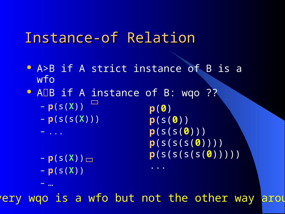
Instance-of RelationInstance-of Relation
A>B if A strict instance of B is a wfo AB if A instance of B: wqo ??
– p(s(X))
– p(s(s(X)))
– ...
– p(s(X))
– p(s(X))
– …
p(0)p(s(0))p(s(s(0)))p(s(s(s(0))))p(s(s(s(s(0)))))...
Every wqo is a wfo but not the other way around
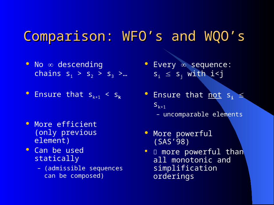
Comparison: WFO’s and WQO’sComparison: WFO’s and WQO’s
No descending chains s1 > s2 > s3 >…
Ensure that sk+1 < sk
More efficient(only previous element)
Can be used statically– (admissible sequences can
be composed)
Every sequence:si sj with i<j
Ensure that not si sk+1
– uncomparable elements
More powerful (SAS’98) more powerful than all
monotonic and simplification orderings

Homeomorphic Embedding Homeomorphic Embedding
Diving: s f(t1,…,tn) if i: s ti
Coupling: f(s1,…,sn) f(t1,…,tn) if i: si ti
n≥0
f(a) g(f(f(a)),a)
f
a
g
a
f
f
a
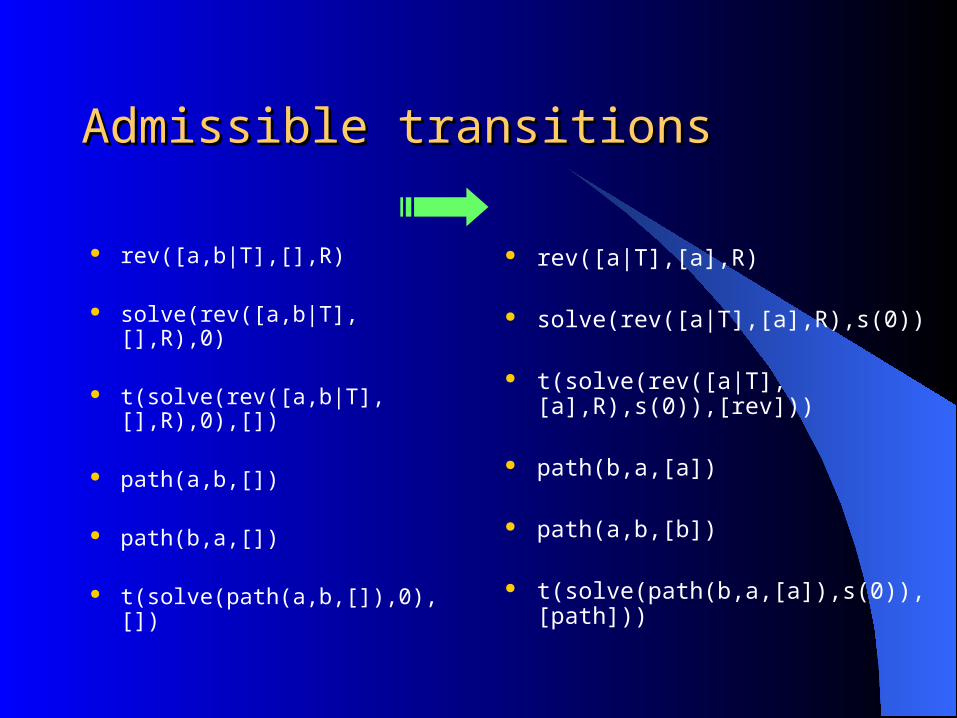
Admissible transitionsAdmissible transitions
rev([a,b|T],[],R)
solve(rev([a,b|T],[],R),0)
t(solve(rev([a,b|T],[],R),0),[])
path(a,b,[])
path(b,a,[])
t(solve(path(a,b,[]),0),[])
rev([a|T],[a],R)
solve(rev([a|T],[a],R),s(0))
t(solve(rev([a|T],[a],R),s(0)),[rev]))
path(b,a,[a])
path(a,b,[b])
t(solve(path(b,a,[a]),s(0)),[path]))

Higman-Kruskal Theorem (1952/60)Higman-Kruskal Theorem (1952/60)
is a WQO (over a finite alphabet) Infinite alphabets + associative operators:
f(s1,…,sn) g(t1,…,tm) if f g andi: si tji
with 1j1<j2<…<jnm
and(q,p(b)) and(r,q,p(f(b)),s)
Variables : X Y more refined solutions possible (DSSE-TR-98-11)
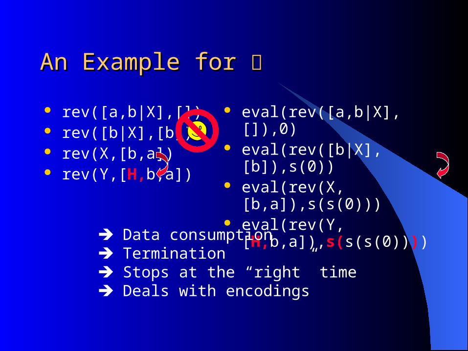
An Example for An Example for
rev([a,b|X],[]) rev([b|X],[b]) rev(X,[b,a]) rev(Y,[H,b,a])
eval(rev([a,b|X],[]),0) eval(rev([b|X],[b]),s(0)) eval(rev(X,[b,a]),s(s(0))) eval(rev(Y,[H,b,a]),s(s(s(0))))
Data consumption Termination Stops at the “right” time Deals with encodings

Summary of part 1Summary of part 1
Local vs Global Control Generic Algorithm Local control:
– Determinacy lookahead code duplication
– Wfo’s
– Wqo’s -homeomorphic embedding

Part 2: Controlling Partial Deduction:Part 2: Controlling Partial Deduction:GlobalGlobal control and control and abstractionabstraction
1. Local Control & Termination2. Global Control & Abstraction

Most Specific Generalisation (msg)Most Specific Generalisation (msg)
A is more general than B iff : B=A
for every B,C there exists a most specific generalisation (msg) M:– M more general than B and C
– if A more general then B and C then A is also more general than M
there exists an algorithm for computing the msg
(anti-unification, least general generalisation)

MSG examplesMSG examples
a a a b X Y
p(a,b) p(a,c) p(a,a) p(b,b)
q(X,a,a) q(a,a,X)
a X X
p(a,X) p(X,X)
q(X,a,Y)

First abstraction operatorFirst abstraction operator
[Benkerimi,Lloyd’90] abstract two atoms in Ai+1 by their msg if they have a common instance
will also ensureindependence(no renaming required)
Termination ?
Input: program P and goal GOutput: specialised program P’Initialise: i=0, A0 = atoms in G
repeat Ai+1 := Ai
for each a Ai do Ai+1 := Ai+1 leaves(unfold(a)) end for Ai+1 := abstract(Ai+1) until Ai+1 = Ai
compute P’ via resultants+renaming

Rev-accRev-accrev([],L,L).rev([H|X],A,R) :- rev(X,[H|A],R).
rev (L,[],R)
rev (L’,[H],R)
rev (L’’,[H’,H],R)
rev (L’,[H],R)
rev (L’’’,[H’’,H’,H],R)
rev (L’’,[H’,H],R)
unfold
unfold
unfold
rev(L,[],R)
rev(L’,[H],R)rev(L’’,[H’,H],R)
rev(L’’’,[H’’,H’,H],R)

First terminating abstractionFirst terminating abstraction
If more than one atom with same predicate in Ai+1: replace them by their msg
{rev (L,[],R), rev (L’,[H],R)} {rev(L,A,R)} Ensures termination
– strict instance-of relation: wfo– either fixpoint or strictly smaller atom
But: loss of precision !– {rev ([a,b|L],[],R), rev (L,[b,a],R)} {rev(L,A,R)}
No specialisation !!

Global treesGlobal trees
Also use wfo’s [MartensGallagher’95] or wqo’s for the global control [SørensenGlück’95, LeuschelMartens’96]
Arrange atoms in Ai+1 as a tree:– register which atoms descend from which
(more precise spotting of non-termination) Only if termination is endangered: apply msg on
the offending atoms– use wfo or wqo on each branch

Rev-accRev-accrev([],L,L).rev([H|X],A,R) :- rev(X,[H|A],R).
rev (L,[],R)
rev (L’,[H],R) rev (L’,[H|A],R)
rev (L,A,R)
unfold unfold
rev(L,[],R)
rev(L’,[H],R)
rev(L,A,R)DANGER
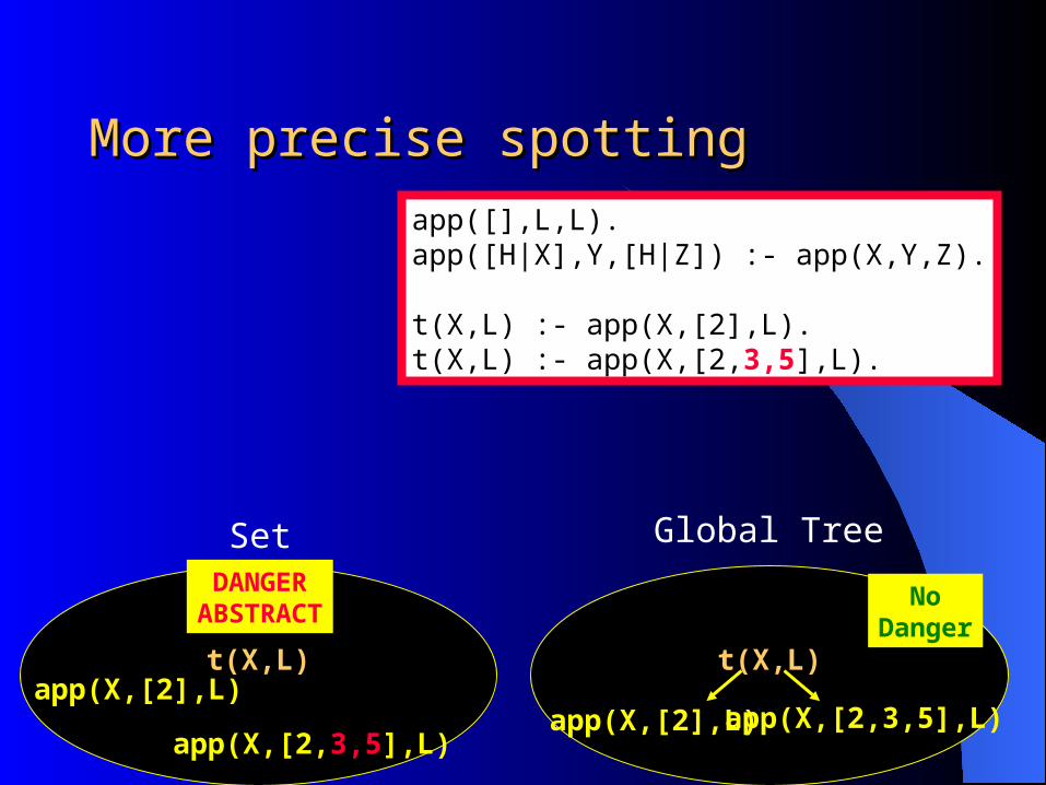
More precise spottingMore precise spotting
app([],L,L).app([H|X],Y,[H|Z]) :- app(X,Y,Z).
t(X,L) :- app(X,[2],L).t(X,L) :- app(X,[2,3,5],L).
t(X,L)app(X,[2],L)
app(X,[2,3,5],L)
t(X,L)
app(X,[2,3,5],L)app(X,[2],L)
Set Global Tree
DANGERABSTRACT
NoDanger

Examining Syntactic StructureExamining Syntactic Structure
p([a],B,C) p(A,[a],C)
abstract: yes or no ???

p=appendp=append
Do not abstract:
app([],L,L).app([H|X],Y,[H|Z]) :- app(X,Y,Z).
app ([a],B,C)
app ([],B,C’)
{C/[a|C’]}
{C’/B}
app (A,[a],C)
app (A’,[a],C’)
{A/[],C/[a]} {A/[H|A’],C/[H|C’]}
app_a([],[a]).app_a([H|A’],[H|C’]) :- app_a(A’,C’).app_a(B,[a|B]).
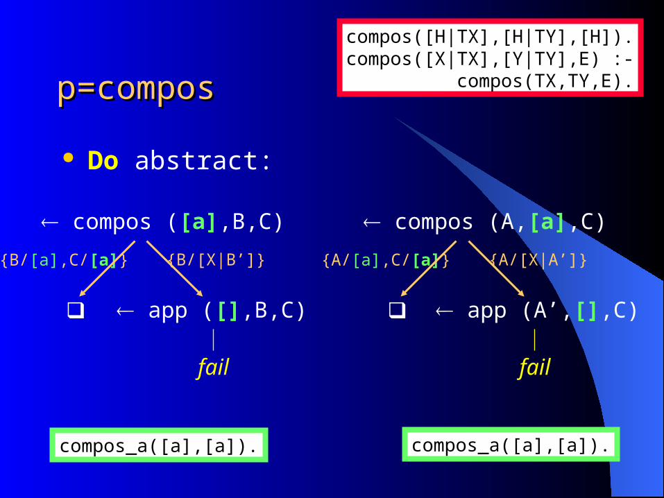
p=composp=compos
Do abstract:
compos([H|TX],[H|TY],[H]).compos([X|TX],[Y|TY],E) :-
compos(TX,TY,E).
compos_a([a],[a]).compos_a([a],[a]).
compos (A,[a],C)
app (A’,[],C)
{A/[a],C/[a]} {A/[X|A’]}
fail
compos ([a],B,C)
app ([],B,C)
{B/[a],C/[a]} {B/[X|B’]}
fail
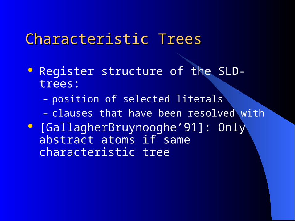
Characteristic TreesCharacteristic Trees
Register structure of the SLD-trees:– position of selected literals
– clauses that have been resolved with [GallagherBruynooghe’91]: Only abstract atoms
if same characteristic tree

Characteristic Trees IICharacteristic Trees II
Abstract: Do not abstract:
Literal 1
Literal 1
Clause 1 Clause 2
fail
Literal 1
Literal 1
Clause 1 Clause 2
fail
Literal 1
stop
Clause 1 Clause 2
Literal 1
Literal 1
Clause 1
Clause 2
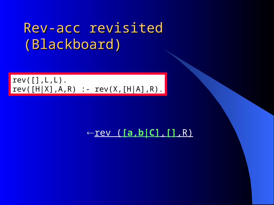
Rev-acc revisited (Blackboard)Rev-acc revisited (Blackboard)
rev([],L,L).rev([H|X],A,R) :- rev(X,[H|A],R).
rev ([a,b|C],[],R)

Path Example (Blackboard)Path Example (Blackboard)
path(A,B,L) :- arc(A,B).path(A,B,L) :-
not(member(A,L)), arc(A,C),path(C,B,[a|L]).
member(X,[X|_]).member(X,[_|L]) :- member(X,L).arc(a,a).
path (a,b,[]) path (a,b,[a])
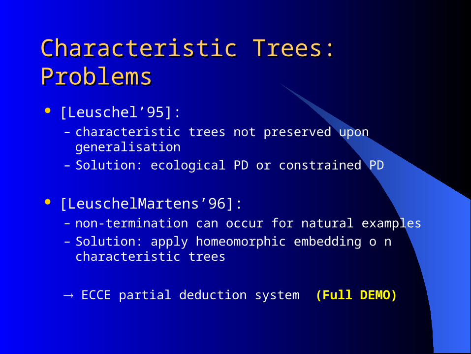
Characteristic Trees: ProblemsCharacteristic Trees: Problems
[Leuschel’95]:– characteristic trees not preserved upon generalisation
– Solution: ecological PD or constrained PD
[LeuschelMartens’96]:– non-termination can occur for natural examples
– Solution: apply homeomorphic embedding o n characteristic trees
ECCE partial deduction system (Full DEMO)

Summary of part 2Summary of part 2
Most Specific Generalisation Global trees
– reusing wfo’s, wqo’s at the global level Characteristic trees
– advantage over purely syntactic structure

Summary of Lectures 2-3Summary of Lectures 2-3
Foundations of partial deduction– resultants, correctness criteria & results
Controlling partial deduction– generic algorithm
– local control: determinacy, wfo’s, wqo’s
– global control: msg, global trees, characteristic trees
04/19/23
Optimisation of Declarative ProgramsOptimisation of Declarative ProgramsLecture 4Lecture 4
Michael Leuschel
Declarative Systems & Software EngineeringDept. Electronics & Computer ScienceUniversity of Southampton
http:// www.ecs.soton.ac.uk/~mal
Part 1:Part 1:A Limitation of Partial DeductionA Limitation of Partial Deduction

SLD-TreesSLD-Trees knows_logic(Z)
good_student(X) teacher(Y,X) logician(Y)
teacher(Y,tom) logician(Y)
logician(peter)
teacher(Y,jane) logician(Y)
Prolog: explores this tree Depth-First, always selects leftmost literal
fail

Partial DeductionPartial Deduction
Basic Principle:– Instead of building one complete SLD-tree:
Build a finite number of finite “SLD- trees” !
– SLD-trees can be incomplete 4 types of derivations in SLD-trees:
– Successful, failed, infinite
– Incomplete: no literal selected
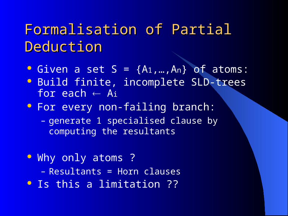
Formalisation of Partial DeductionFormalisation of Partial Deduction
Given a set S = {A1,…,An} of atoms: Build finite, incomplete SLD-trees for each Ai
For every non-failing branch:– generate 1 specialised clause by
computing the resultants
Why only atoms ?– Resultants = Horn clauses
Is this a limitation ??

Control:Control:Local vs GlobalLocal vs Global Local Control:
– Decide upon the individual SLD-trees– Influences the code generated for each Ai
unfolding rule given a program P and goal G returns finite, possibly
incomplete SLD-tree
Global control– decide which atoms are in A
abstraction operator
A1 A2 A3 A4 ...
A

Generic AlgorithmGeneric Algorithm
Input: program P and goal GOutput: specialised program P’Initialise: i=0, A0 = atoms in G
repeat Ai+1 := Ai
for each a Ai do Ai+1 := Ai+1 leaves(unfold(a)) end for Ai+1 := abstract(Ai+1) until Ai+1 = Ai
compute P’ via resultants+renaming

Limitation 1: Side-ways InformationLimitation 1: Side-ways Information
t(X) :- p(X), q(X).
p(a).
q(b).
t(Y)
p(Y),q(Y)
{Y/a}
p(Y)
{Y/b}
q(Y)
Original program !

Limitation 1: Solution ?Limitation 1: Solution ?
t(X) :- p(X), q(X).
p(a).
q(b).
Just unfold deeper
t(Y)
p(Y),q(Y)
q(a)
fail
t(X) :- fail.

Limitation 1: Solution ?Limitation 1: Solution ?
t(X) :- p(X), q(X).
p(a).
p(X) :- p(X).
q(b).
We cannot fullyunfold !!
t(Y)
p(Y),q(Y)
q(a)
fail
p(Y),q(Y)

Limitation 1Limitation 1
Side-ways information passing– solve(Call,Res),manipulate(Res)
Full unfolding not possible:– termination (e.g. of Res)
– code explosion
– efficiency (work duplication) Ramifications:
– difficult to automatically specialise interpreters(aggressive unfolding required)
– no tupling, no deforestation

Limitation 1: SolutionsLimitation 1: Solutions
Pass least upper bound around– For a query A,B:
Take msg of all (partial) solutions of A Apply msg to B
Better:– Specialise conjunctions instead of atoms
Conjunctive Partial Deduction

Part 2:Part 2:Conjunctive Partial DeductionConjunctive Partial Deduction

Conjunctive Partial DeductionConjunctive Partial Deduction
Given a set S = {C1,…,Cn} of atoms: Build finite, incomplete SLD-trees for each Ci
For every non-failing branch:– generate 1 specialised formula Ci L by
computing the resultants To get Horn clauses
– Rename conjunctions into atoms !
Assign every Ci an atom with the same variables and each with a different predicate name

Renaming FunctionRenaming Function
p(f(X)),q(b) p(X),q(X)
p(f(X)),q(b) p(X),r(X),q(X)
p(Y),q(Y)
rename
pq(Y)
pq(f(X),b) pq(X)
pq(f(X),b) pq(X), r(X) orpq(f(X),b) r(X), pq(X)
Resolve ambiguities contiguous: if no reordering allowed

Soundness & CompletenessSoundness & Completeness
P’ obtained by conjunctive partial deduction from P
If non-triviality, closedness wrt renaming function: P’ {G} has an SLD-refutation with c.a.s.
iff P {G}hasIf in addition fairness (or weak fairness): P’ {G} has a finitely failed SLD-tree iff
P {G}has see Leuschel et al: JICSLP’96

Maxlength Example (Blackboard)Maxlength Example (Blackboard)
max_length(X,M,L) :- max(X,M),len(X,L).max(X,M) :- max(X,0,M).max([],M,M).max([H|T],N,M) :- H=<N,max(T,N,M).max([H|T],N,M) :- H>N,max(T,H,M).len([],0).len([H|T],L) :- len(T,TL),L is TL+1.
maxlen (X,M,L)
max(X,N,M),len(X,L)
rename
ml(X,N,M,L)

Double-Append Example Double-Append Example (blackboard)(blackboard)app([],L,L).app([H|X],Y,[H|Z]) :- app(X,Y,Z).
app (A,B,I), app(I,C,Res)
da([],B,B,C,Res) :- app(B,C,Res).da([H|A’],B,[H|I’],C,[H|R’]) :- da(A’,B,I’,C,R’).
da([],B,C,Res) :- app(B,C,Res).da([H|A’],B,C,[H|R’]) :- da(A’,B,C,R’).
??
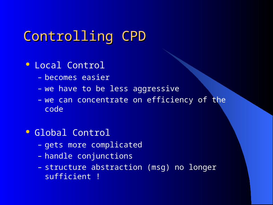
Controlling CPDControlling CPD
Local Control– becomes easier
– we have to be less aggressive
– we can concentrate on efficiency of the code
Global Control– gets more complicated
– handle conjunctions
– structure abstraction (msg) no longer sufficient !

Global Control of CPDGlobal Control of CPD
p(0,0). p(f(X,Y),R) :- p(X,R),p(Y,R).
Specialise p(Z,R) We need splitting How to detect infinite branches:
– homeomorphic embedding on conjunctions How to split:
– most specific embedded conjunction

Homeomorphic Embedding on Conj.Homeomorphic Embedding on Conj.
Define: and/m and/n
f(s1,…,sn) g(t1,…,tm) if f g andi: si tji
with 1j1<j2<…<jnm
and(q,p(b)) and(r,q,p(f(b)),s)

Most Specific Embedded Subconj.Most Specific Embedded Subconj.
p(X) q(f(X))
t(Z) p(s(Z)) q(a) q(f(f(Z)))
{ t(Z), q(a), p(s(Z)) q(f(f(Z))) }
Splitting

Generic AlgorithmGeneric Algorithm
Plilp’96, Lopstr’96, JLP’99
Input: program P and goal GOutput: specialised program P’Initialise: i=0, A0 = {G}
repeat Ai+1 := Ai
for each c Ai do Ai+1 := Ai+1 leaves(unfold(c)) end for
Ai+1 := abstract(Ai+1) until Ai+1 = Ai
compute P’ via resultants+renaming
Changesover PD
Don’tseparate intoatoms
Msg +splitting
Ecce demo of conjunctive partial Ecce demo of conjunctive partial deductiondeduction Max-length Double append
depth, det. Unf. with PD and CPD
rotate-prune

Comparing with FPComparing with FP
Conjunctions– can represent nested function calls (supercompilation
[Turchin], deforestation [Wadler])g(X,RG),f(RG,Res) = f(g(X))
– can represent tuples (tupling [Chin])g(X,ResG),f(X,ResF) = f(X),g(X)
We can do both deforestation and tupling !– No such method in FP
Semantics for infinite derivations (WFS) in LP– safe removal of infinite loops, etc…
– applications: interpreters,model checking,...
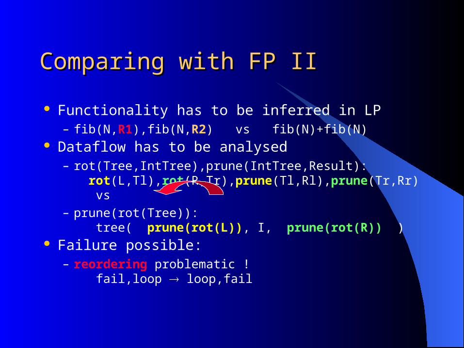
Comparing with FP IIComparing with FP II
Functionality has to be inferred in LP– fib(N,R1),fib(N,R2) vs fib(N)+fib(N)
Dataflow has to be analysed– rot(Tree,IntTree),prune(IntTree,Result):
rot(L,Tl),rot(R,Tr),prune(Tl,Rl),prune(Tr,Rr) vs
– prune(rot(Tree)): tree( prune(rot(L)), I, prune(rot(R)) )
Failure possible:– reordering problematic !
fail,loop loop,fail

Part 3:Part 3:Another Limitation of Partial Another Limitation of Partial Deduction (and CPD)Deduction (and CPD)

Limitation 2: Global Success Limitation 2: Global Success InformationInformation
p(a).
p(X) :- p(X).
We get sameprogram back
The fact that in all successful derivations X=a is not explicit !
p(Y)
p(Y)

Limitation 2: Failure exampleLimitation 2: Failure example
t(X) :- p(X), q(X).
p(a).
p(X) :- p(X).
q(b). Specialised program:
t(X) :- pq(X).
pq(X) :- pq(X).
But even better:t(X) :-fail.
t(Y)
p(Y),q(Y)
q(a)
fail
p(Y),q(Y)
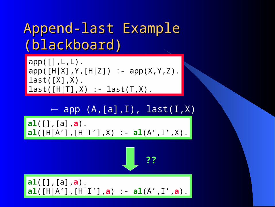
Append-last Example (blackboard)Append-last Example (blackboard)
app([],L,L).app([H|X],Y,[H|Z]) :- app(X,Y,Z).last([X],X).last([H|T],X) :- last(T,X).
app (A,[a],I), last(I,X)
al([],[a],a).al([H|A’],[H|I’],X) :- al(A’,I’,X).
al([],[a],a).al([H|A’],[H|I’],a) :- al(A’,I’,a).
??
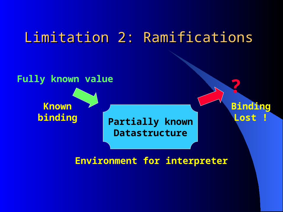
Limitation 2: RamificationsLimitation 2: Ramifications
Partially knownDatastructure
Fully known value?
Environment for interpreter
Knownbinding
BindingLost !
Part 4:Part 4:Combining Abstract Interpretation Combining Abstract Interpretation with (Conjunctive) Partial Deductionwith (Conjunctive) Partial Deduction
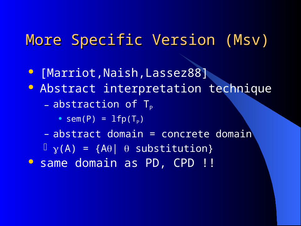
More Specific Version (Msv)More Specific Version (Msv)
[Marriot,Naish,Lassez88] Abstract interpretation technique
– abstraction of TP
sem(P) = lfp(TP)
– abstract domain = concrete domain (A) = {A| substitution}
same domain as PD, CPD !!

TTPP operator operator
Head :- B1, B2, …, Bn.
Head 1…n
A
DC H
B
E
GF
1
n
Head1…n
S
TP(S)
TTPP operator operator
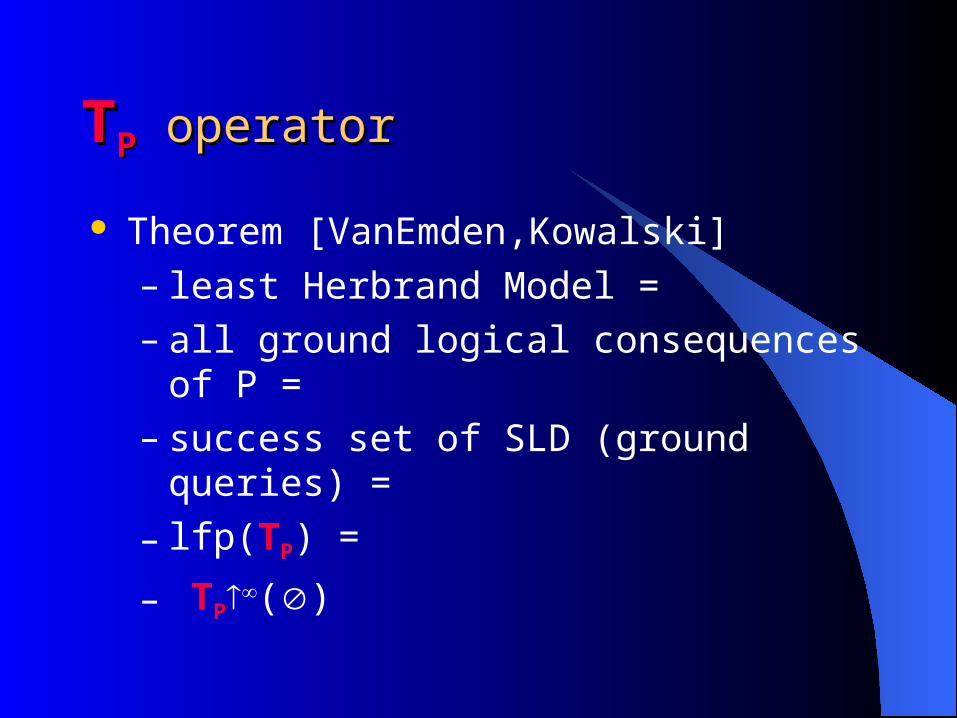
Theorem [VanEmden,Kowalski]
– least Herbrand Model = – all ground logical consequences of P =– success set of SLD (ground queries) =
– lfp(TP) =
– TP()
TTPP operator: Example operator: Example
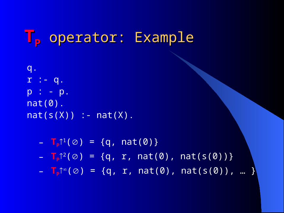
q.r :- q.p : - p.nat(0).nat(s(X)) :- nat(X).
– TP1() = {q, nat(0)}
– TP2() = {q, r, nat(0), nat(s(0))}
– TP() = {q, r, nat(0), nat(s(0)), … }

Abstraction of TPAbstraction of TP
Compose TP with predicate-wise msg Ensures terminationq.r :- q.p : - p.nat(0).nat(s(X)) :- nat(X).
– TP1() = {q, nat(0)}
– TP2() = {q, r, nat(0), nat(s(0))}
– TP*2() = TP*() = {q, r, nat(X)}
Msg = nat(X)

More Specific Version: PrinciplesMore Specific Version: Principles
Compute S = TP*() For every body atom of the program:
– unify with an element of S – if none exists: clause can be removed !
The resulting program is called a more specific version of P
Correctness:– computed answers preserved– finite failure preserved– infinite failure can be replaced by finite failure

MSV applied to append-lastMSV applied to append-last
TP1() = {al([],[a],a)}
TP2() = {al([],[a],a), al([H],[H,a],a)}
TP*2() = {al(L,[X|Y],a)}
TP (TP*2()) = {al([],[a],a), al([H|L],[H,X|Y],a)}
TP*3() = TP*() = {al(L,[X|Y],a)}
al([],[a],a).al([H|A’],[H|I’],X) :- al(A’,I’,X).
al([],[a],a).al([H|A’],[H,H’|I’],a) :- al(A’,[H’|I’],a).
MSVNote: msv on originalprogram gives no result !!

Naïve CombinationNaïve Combination
repeat– Conjunctive Partial Deduction
– More Specific Version until fixpoint (or we are satisfied)
Can be done with ecce Power/Applications:
– cf. Demo (later in the talk)
– interpreters for the ground representation

Even-Odd example (blackboard)Even-Odd example (blackboard)
even(0).even(s(X)) :- odd(X).odd(s(X)) :- even(X).eo(X) :- even(X),odd(X).
Msv alone: not sufficient !
Specialise eo(X) + msv:– eo(X) :- fail.

Refined AlgorithmRefined Algorithm
[Leuschel,De Schreye Plilp’96]
Specialisation continued before fixpoint of msv is reached !
Required when several predicates interact– E.g.: for proving functionality of multiplication

ITP example (demo)ITP example (demo)
plus(0,X,X).plus(s(X),Y,s(Z)) :- plus(X,Y,Z).
pzero(X,XPlusZero) :- plus(X,0,XPlusZero).
passoc(X,Y,Z,R1,R2) :- plus(X,Y,XY),plus(XY,Z,R1),
plus(Y,Z,YZ),plus(X,YZ,R2).
=X !
=R1 !
Model Checking ExampleModel Checking Example
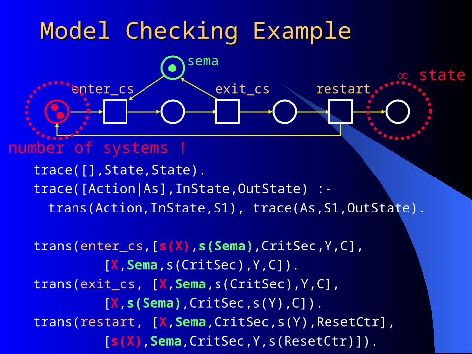
trace([],State,State).
trace([Action|As],InState,OutState) :-
trans(Action,InState,S1), trace(As,S1,OutState).
trans(enter_cs,[s(X),s(Sema),CritSec,Y,C],
[X,Sema,s(CritSec),Y,C]).
trans(exit_cs, [X,Sema,s(CritSec),Y,C],
[X,s(Sema),CritSec,s(Y),C]).
trans(restart, [X,Sema,CritSec,s(Y),ResetCtr],
[s(X),Sema,CritSec,Y,s(ResetCtr)]).
sema
restartexit_csenter_cs state !
number of systems !
Model Checking continuedModel Checking continued
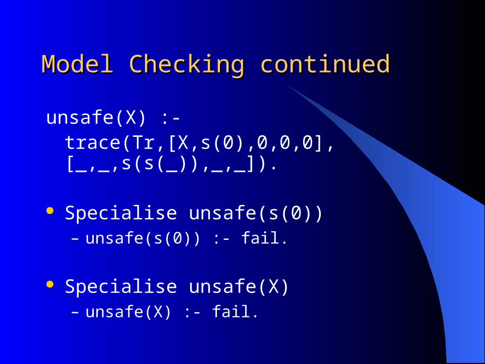
unsafe(X) :-trace(Tr,[X,s(0),0,0,0],[_,_,s(s(_)),_,_]).
Specialise unsafe(s(0))– unsafe(s(0)) :- fail.
Specialise unsafe(X)– unsafe(X) :- fail.

Ecce + Msv DemoEcce + Msv Demo
Append last Even odd (itp) pzero (itp) passoc (itp) Infinite Model Checking (petri2)

Full ReconicilationFull Reconicilation
Why restrict to simple abstract domain– ( = all instances)
Why not use– groundness dependencies
– regular types
– type graphs p(0)
p(s(0))Better: p() ; = 0|s()
Msg = p(X)
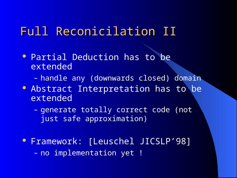
Full Reconicilation IIFull Reconicilation II
Partial Deduction has to be extended– handle any (downwards closed) domain
Abstract Interpretation has to be extended– generate totally correct code (not just safe
approximation)
Framework: [Leuschel JICSLP’98]– no implementation yet !

Summary of Lecture 4Summary of Lecture 4
Conjunctive partial deduction– better precision
– tupling
– deforestation More Specific Versions
– simple abstract interpretation technique Combination of both
– powerful specialiser/analyser
– infinite model checking


![DECEMBER 2018 Declarative or Imperative Language · Declarative or Imperative Language [Abraham John, Executive Director, AITS] ... declarative languages are typically cleaner, better](https://static.fdocuments.in/doc/165x107/5ec7e462e396e9508e214783/december-2018-declarative-or-imperative-language-declarative-or-imperative-language.jpg)


![Declarative tools [for] connecting softwareusers.dsic.upv.es/workshops/euindia05/slides/slucas.pdf · Connecting declarative software tools Declarative tools [for] connecting software](https://static.fdocuments.in/doc/165x107/5b79a4a17f8b9a7f378e158d/declarative-tools-for-connecting-connecting-declarative-software-tools-declarative.jpg)