Optimal transaction filters under transitory trading...

ARTICLE IN PRESS

Journal of Financial Markets 13 (2010) 129–156

1386-4181/$ -

doi:10.1016/j

�CorrespoWest Virgini

E-mail ad

www.elsevier.com/locate/finmar

Optimal transaction filters under transitory tradingopportunities: Theory and empirical illustration

Ronald Balversa,c,�, Yangru Wub,c

aDivision of Economics and Finance, College of Business and Economics, West Virginia University,

Morgantown, WV 26506, USAbRutgers Business School-Newark and New Brunswick, Rutgers University, Newark, NJ 07102, USAcChinese Academy of Finance and Development, Central University of Finance and Economics, China

Available online 5 August 2009

Abstract

If transitory profitable trading opportunities exist, transaction filters mitigate trading costs. We use

a dynamic programming framework to design an optimal filter that maximizes after-cost expected

returns. The filter size depends crucially on the degree of persistence of trading opportunities,

transaction cost, and standard deviation of shocks. For daily dollar–yen exchange trading, the

optimal filter can be economically significantly different from a naı̈ve filter equal to the transaction

cost. The candidate trading strategies generate positive returns that disappear after transaction costs.

However, when the optimal filter is used, returns after costs remain positive and higher than for naı̈vefilters.

r 2009 Elsevier B.V. All rights reserved.

JEL classification: G10; G15; G11

Keywords: Transaction costs; Transaction filters; Trading strategies; Foreign exchange

1. Introduction

It is inarguable that opportunities for above-normal returns are available to marketparticipants at some level. These opportunities may be exploitable for instance at an intra-daily frequency as a reward for information acquisition when markets are efficient, or at a

see front matter r 2009 Elsevier B.V. All rights reserved.

.finmar.2009.07.005

nding author at: Division of Economics and Finance, College of Business and Economics,

a University, Morgantown, WV 26506, USA. Tel.: +1 304 293 7880; fax: +1 304 293 2233.

dresses: [email protected] (R. Balvers), [email protected] (Y. Wu).

www.elsevier.com/locate/finmar

dx.doi.org/10.1016/j.finmar.2009.07.005

mailto:[email protected]

mailto:[email protected]

ARTICLE IN PRESSR. Balvers, Y. Wu / Journal of Financial Markets 13 (2010) 129–156130

lower frequency to market timers when markets are inefficient. By nature these profitopportunities are predicable but transitory, and transaction costs may be a majorimpediment in exploiting them.1 This paper explores the optimal trading strategy whentransitory opportunities exist and transactions are costly.The model we present is applicable to the arbitrage of microstructure inefficiencies that

require frequent and timely transactions, which may be largely riskless. An example isuncovered interest speculation in currency markets where a trader takes either one side ofthe market or the reverse. Alternatively, a trader arbitrages differences between an asset’sreturn and that of one of its derivatives: going long on the arbitrage position or reversingthe position and going short, as is the case in covered interest arbitrage.Alexander (1961) and Fama and Blume (1966) introduced ‘‘filter rules’’ according to

which traders buy (sell) an asset only if its current price exceeds (is below) the previouslocal minimum (maximum) by more than X (more than Y) percent, where X and Y areparameters of the rule, commonly set equal and chosen in the range of 0.5–5% (e.g.,Sweeney, 1986). The parameters X (and Y if different) determine a ‘‘band of inactivity’’that prompts one to trade once a realization exceeds the local minimum or is below thelocal maximum by a certain percentage. A larger band of inactivity (larger X) filters outmore trades, thus reducing transactions costs.2 The general idea of filters, in filter rules, aswell as other trading rules, is that if the trade indicator is weak the expected return fromthe transaction may not compensate for the transaction cost. Lehmann (1990) provides aninteresting alternative filter by varying portfolio weights according to the strength of thereturn indicators—in trading smaller quantities of the assets with the weaker tradeindicators, transaction costs are automatically reduced relative to the payoff.Knez and Ready (1996) and Cooper (1999) explore different filters and find that the

after-transaction-cost returns indeed improve compared to trading strategies with zerofilter. The problem with the filter approach is that there is no way of knowing a prioriwhich filter band is reasonable because the buy/sell signal and the transaction cost are notin the same units—the filter is the percentage by which the effective signal exceeds thesignal at which a change in position first appears profitable before transaction costs, butthis percentage bears no relation to the percentage return expected. This also implies thatthere is no discipline against data mining for researchers: many filters with different bandscan be tried to fabricate positive net strategy returns. While Lehmann’s (1990) approachprovides more discipline as it specifies a unique strategy, the filter it implies is not generallyoptimal.The purpose of this paper is to design an optimal filter that a priori maximizes the

expected return net of transaction cost. To accomplish this we employ a ‘‘parametric’’approach (e.g., Balvers et al., 2000) that allows the trading signal and the transaction cost

1For instance, Grundy and Martin (2001) express doubt that the anomalous momentum profits survive

transaction costs, and Hanna and Ready (2005) find that the momentum profits are substantially reduced when

transaction costs are accounted for. Lesmond et al. (2004) conclude more strongly that momentum profits with

transaction costs are illusory. Neely and Weller (2003) reach a similar conclusion for trading profits in foreign

exchange markets after transaction costs.2Note the two usages of the term filter. We distinguish ‘‘filter rules’’—the specific class of technical trading rules

defined above—from a more generic use of the term ‘‘filter’’—a criterion for selecting a set of trades to exclude.

The latter refers typically to a ‘‘band of inactivity’’. Filter rules use different size filters but filters can be applied to

a much broader class of trading rules that are not filter rules. In the following we examine different size filters for

ARMA and moving average trading rules, but not for filter rules.

ARTICLE IN PRESSR. Balvers, Y. Wu / Journal of Financial Markets 13 (2010) 129–156 131

to be in the same units. In effect we convert a filter into returns space and then are able toderive the filter’s optimal band. The optimal filter depends on the exact balance betweenmaintaining the most profitable transactions and minimizing the transactions costs.

The optimal filter (band) can be no larger than the transaction cost (plus interest). This isclear because there is no reason to exclude trades that have an immediate expected returnlarger than the transaction cost. In general, the optimal filter is significantly smaller thanthe transaction cost. This occurs when the expected return is persistent: even if theimmediate return from switching is less than the transaction cost, the persistence of theexpected return makes it likely that an additional return is foregone in future periods bynot switching. Roughly, the filter must depend on the transaction cost, as well as a factorrelated to the probability that a switch occurs. Our model characterizes the determinants ofthe filter in general and provides an exact solution for the filter when zero-investmentreturns have a uniform distribution.

In exploring the effect of transaction costs when returns are predictable, this paper hasthe same objective as Balduzzi and Lynch (1999), Lynch and Balduzzi (2000), and Lynchand Tan (2009).3 The focus of these authors, however, differs significantly from ours inthat they consider the utility effects and portfolio rebalancing decisions, respectively, in alife cycle portfolio choice framework. They simulate the welfare cost and portfoliorebalancing decisions given a trader’s constant relative risk aversion utility function, butthey do not provide analytical solutions and it is difficult to use their approach to quantifythe optimal trading strategies for particular applications. Our approach, in contrast,provides specific theoretical results yielding insights into the factors affecting optimaltrading strategies. Moreover, our results can be applied based on observable marketcharacteristics that do not depend on subjective utility function specifications.

In contrast to Balduzzi and Lynch (1999), Lynch and Balduzzi (2000), and Lynch andTan (2009), we sidestep the controversial issue of risk in the theory. This simplifies ouranalysis considerably and is reasonable in a variety of circumstances. First, we can thinkof the raw returns as systematic-risk-adjusted returns, with whichever risk model isconsidered appropriate. The systematic risk adjustment is sufficient to account for all riskas long as trading occurs at the margins of an otherwise well-diversified portfolio. Second,in particular at intra-daily frequencies, traders may create arbitrage positions so that risk isirrelevant. Third, in many applications risk considerations are perceived as secondarycompared to the gains in expected return; if risk adjustments are relatively small so that theoptimal trading rules are approximately correct then risk corrections can be safely appliedto ex post returns.

Our optimal filter will produce higher expected returns than the naı̈ve strategies of eitherusing no filter or using a transaction-cost-sized filter. We apply the optimal filter to anatural case for our model: daily foreign exchange trading in the yen/dollar market. As iswell-known (e.g., Cornell and Dietrich, 1978; Sweeney, 1986; LeBaron, 1998; Gencay,1999; Qi and Wu, 2006), simple moving-average trading rules improve forecasts ofexchange rates and generate positive expected returns (with or without risk adjustment) in

3There is a far more extensive literature considering investment choices under transaction costs when returns are

not predictable. See Liu and Loewenstein (2002) and Liu (2004) for recent examples. Marquering and Verbeek

(2004) assume predictability and adjust for transaction costs. Their approach, however, is a complement to ours in

that they integrate risk into the optimal switching choice while accounting for transaction costs after the fact,

whereas our approach integrates transaction costs into the optimal switching choice while accounting for risk after

the fact.


the foreign exchange market. However, for daily trading, returns net of transaction costsare negative or insignificant if no filter is applied (Neely and Weller, 2003).4

We find that for the optimal filter, the net returns are still significantly positive andhigher than those when the filter is set equal to the transaction cost. Further, the optimalfilter derived from the theory given a uniform distribution and two optimal filters derivednumerically under normality and bootstrapping assumptions all generate similar resultsthat are relatively close to the ex post maximizing filter for actual data. These results areimportant as they suggest an approach for employing trading strategies with filters to dealwith transaction costs, without inviting data mining. The results also hint that in somecases the conclusion that abnormal profits disappear after accounting for transaction costsmay be worth revisiting.Section 2 develops the theoretical model and provides a general characterization of the

optimal filter for an ARMA(1,1) returns process with general shocks, as well as a specificformula for the case when the shocks follow the uniform distribution. In Section 3, weapply the model to uncovered currency speculation. We show first that the moving-averagestrategy popular in currency trading can be related to our ARMA(1,1) specification. Wethen use the first one-third of our sample to develop estimates of the returns process, whichwe employ to calculate the optimal filter for an ARMA(1,1), an AR(1), and tworepresentative MA returns processes. The optimal filter is obtained from the theoreticalmodel for the uniform distribution but also numerically for the normal distribution andthe bootstrapping distribution. In Section 4, we conduct the out-of-sample test with thefinal two-thirds of the sample to compare mean returns from a switching strategy beforeand after transaction costs. The switching strategies are conducted under a variety offilters, including the optimal ones, for each of the ARMA(1,1), AR(1), and MA returnscases. Section 5 concludes the paper.

2. The theoretical model

2.1. Autoregressive conditional returns and two risky assets

An individual investor maximizes the discounted expected value of an investment overthe infinite horizon. There is a proportional transaction cost and the investor chooses ineach period between two assets that have autocorrelated mean returns. Each period, theinvestor is assumed to take a zero-cost investment position: a notional $1 long position inone asset and a notional $1 short position in the other. This implies that any profits orlosses do not affect future investment positions. The return on the zero-cost investmentposition xt (a $1 long position in asset 1 and a $1 short position in asset 2) is assumed tofollow an ARMA(1,1) process as a parsimonious parameterization of mild returnpredictability. Given that either the return on the investment position has no systematicrisk or the investor is risk neutral, the decision problem is

V 1ðxt�1; �t�1Þ ¼ Et�1 xt þMaxV 1ðxt; �tÞ

1þ r;V 2ðxt; �tÞ

1þ r� 2c

� �� (1)

4Gencay et al. (2002) show that real time trading models that employ more sophisticated techniques than the

simple moving average rules can generate positive cost-adjusted returns with intra-day data.


subject to

xt ¼ rxt�1 � d�t�1 þ �t; Et�1�t ¼ 0; r4Maxð0; dÞ. (2)

Each period, the investor chooses whether to hold a zero-investment position long in asset1 and short in asset 2, or the reverse. A proportional transaction cost c is incurredwhenever a position is closed out, implying a cost of 2c when a position is reversed.5 InEq. (1), the expected net present value (NPV) of the investment strategy denoted by thevalue function V ið�Þ at time t�1 depends on the state as given by the existing long positionin asset i and short position in the other asset, and the variables describing the distributionof xt, namely xt�1 and �t�1. This value equals the current expected return, given the existingasset position (which we call 1 without loss of generality), plus the expected value in thenext period discounted once at rate r, which depends on the updated return state variablesxt and �t, as well as the new zero-investment asset position (i ¼ 1 or 2, whichevermaximizes the expected NPV), and minus the up-front adjustment cost incurred if the zero-investment position is switched from long in asset 1 to long in asset 2. Wealth is not a statevariable, because of risk neutrality and the assumption that the long position in eachperiod is always $1. Assuming that the scale of investment is low enough that wealth/margin does not become an issue preserves the relative simplicity of the decision problem.

Eq. (2) describes the return process xt for the zero-investment position long in asset 1and short in asset 2. The ARMA(1,1) process for xt is assumed to be persistent in the sensethat xt�1 positively affects xt (r40) and that �t�1 positively affects xt (r4d). Theunconditional mean of xt is zero and reversing the zero-cost position necessarily generatesa return of �xt. Define mt � Et�1xt, and let it represent, without loss of generality, theconditional expected return of the current zero-investment position. The disturbance term�t is symmetric and unimodal, with unbounded support, density f ð�tÞ, and cumulativedensity F ð�tÞ. V ð�Þ denotes the maximum expected NPV of the strategy given the existingzero-investment position. Then:

Proposition 1. For the decision problem in Eqs. (1) and (2) a unique m�o0 exists such that

the investor maintains the current zero-investment position whenever mtþ14m� and reverses

the position whenever mtþ1 � m�. The resulting expected NPV is

V ðmtÞ ¼ mt þ

Z 1ðm��rmtÞ=ðr�dÞ

V ðmtþ1Þ

1þ r

� �dF ð�tÞ þ

Z ðm��rmtÞ=ðr�dÞ

�1

V ð�mtþ1Þ

1þ r� 2c

� �dF ð�tÞ

(3)

subject to

mtþ1 ¼ rmt þ ðr� dÞ�t with Et�1�t ¼ 0; r4Maxð0; dÞ. (4)

Proof. See Appendix A.

Eq. (3) states that the maximum expected discounted investment return is equal to theexpected return for the current position mt plus, either the once-discounted maximumexpected NPV of the strategy when the current investment position is maintained, or theonce-discounted maximum expected NPV of the strategy, net of adjustment costs incurredwhen the current investment position is reversed. The integral bounds indicate the critical

5Given the assumed risk neutrality, symmetry, and proportional transaction costs, intermediate positions, with

investment in both assets or in neither asset, are never optimal.


(cutoff) value for the current disturbance term �t according to which the investmentposition is maintained or reversed (higher �t implies higher future expected return for theexisting zero-investment position, so less incentive to switch). mt is a sufficient state variablefor the individual investor maximizing the expected NPV from the zero-cost investmentpositions because Eq. (2) for the realized zero-investment return implies Eq. (4) for theconditional expected zero-investment return, and the latter is the pertinent variable for therisk-neutral expected value maximizer.Given the benefit of switching, the difference between V ð�mÞ and V ðmÞ is monotonically

decreasing in m, there is exactly one critical value m� below which switching is optimal.Intuitively m� must be negative because it makes no sense to switch when mtþ1 is zero orpositive. Our purpose is to provide in the following a specific characterization of m� forempirical purposes.To examine the specific advantage from switching the asset position, take the difference

between the value of long in one asset and short in the other after a switch, V ð�mÞ, and theinitial position, V ðmÞ:

V ð�mtÞ � V ðmtÞ ¼ �2mt þ BðmtÞ þ CðmtÞ. (5)

Eq. (5) follows directly from applying Eq. (3) twice, for �mt and mt, and manipulating theintegrals (as shown in Appendix A). The first term on the right-hand side indicates thedirect benefit of switching from mt to �mt. The second term, BðmtÞ, is given as

BðmtÞ ¼

Z ð�m��rmtÞ=ðr�dÞ

ðm��rmtÞ=ðr�dÞ

V ð�mtþ1Þ � V ðmtþ1Þ

1þ r

� �dF ð�tÞ. (6)

BðmtÞ represents the future benefit of switching now, given that neither of the two possiblepositions (the current available choices) would be switched in the next period. The integralbounds equal the critical values for et at which a switch takes place (lower bound forswitching next period when having switched in the previous period; upper bound forswitching next period when not having switched previously). Use Eq. (4) to see that thedifference V ð�mtþ1Þ � V ðmtþ1Þ on the right-hand side of Eq. (6) is evaluated from þm� to�m�. The symmetry of this difference further implies that the sign depends only on theshape of the density function. In particular, taking m�o0 (which is always so, as we showshortly), if mto0 then the range over which V ð�mtþ1Þ � V ðmtþ1Þ is negative (whenevermtþ140) is weighted less than the range over which it is positive, because the density issymmetric and unimodal (vice versa if mt40). Thus BðmtÞ is always strictly positive formto0, unless the density function is flat (as is the case for the uniform distribution). Thethird term in Eq. (5), CðmtÞ, is given as

CðmtÞ ¼ 2c


ðm�þrmtÞ=ðr�dÞdF ð�tÞ ¼ 2c F

m� � rmt

r� d

� �� F

m� þ rmt

r� d

� �� . (7)

It gives the future benefit of switching now, given that for one of the two possible positionsit will be optimal to switch in the next period (note that it is never optimal for bothpositions to switch). In that case, both possible positions end up becoming identical oneperiod later and the only difference is the transaction cost. CðmtÞ represents the expecteddifference in transaction cost expenditure for the two positions: the cost times theprobability of not switching initially but switching anyway next period minus the


probability of switching initially and then switching back in the next period. Note that,from inspection of Eq. (7), CðmtÞ must be positive for mto0 (and negative for mt40).

To determine the critical value m� we evaluate Eq. (5) for mt ¼ m�. First consider that m�

is determined optimally. Since the integral bounds are chosen optimally to obtain themaximum expected NPV from the investment strategy, it must be that the derivative withrespect to the bound in Eq. (3) is zero. Using Leibniz’s rule to obtain the first-ordercondition for m� in Eq. (3) gives

V ð�m�Þ1þ r

�V ðm�Þ1þ r

¼ 2c. (8)

Eq. (8) reveals that the critical return is determined at the point where the total presentvalue of expected benefit from reversing the investment position is exactly equal to theupfront transaction cost: at mtþ1 ¼ m�o0 the investor is indifferent between maintainingthe current investment position with negative expected return m� next period and reversingthe investment position that has an immediate transaction cost of 2c but a positiveexpected next-period return �m�. It is directly clear from Eq. (8) that m* must be constantover time, as its notation without time subscript presumes.

Evaluate Eq. (5) at mt ¼ m� and use Eq. (8) to obtain6:

m� ¼ �cð1þ rÞ þ 12½Bðm�Þ þ Cðm�Þ�. (9)

Intuitively, Eq. (9) sets the critical expected return m� equal to the benefit of switchingpositions at m� minus the up-front transaction cost (including interest) from switching. Thebenefit of switching at the expected return m� includes the cost saving of a reduction in theprobability of switching next period, Cðm�Þ, as well as the expected immediate revenuefrom the improved asset position, Bðm�Þ. As Bðm�Þ þ Cðm�Þ40 from Eqs. (6) and (7), giventhat m�o0, it follows that �m�ocð1þ rÞ. This is intuitive because, if the current expectedreturn is greater than or equal to the transaction cost, a switch is clearly beneficial becausethe end-of-period gain in expected return �2m� immediately pays for the transaction cost2cð1þ rÞ while the switch also improves the potential for future profits.

2.2. Closed form solution for uniform innovations

It is difficult to obtain an explicit analytical solution for the optimal filter in Eq. (9)because, from Eq. (6), Bðm�Þ depends on the value function, which is of unknownfunctional form. However, for the special case of a constant density over the relevant range(a uniform distribution), the Bðm�Þ term simplifies substantially, as shown in the following,so that an explicit solution can be obtained.

Assume a uniform distribution for e over the interval ½�z; z� with implied densityf ð�Þ ¼ 1=ð2zÞ. To apply to this case, Proposition 1 requires minor modifications, whichwe omit for brevity, since the uniform distribution is bounded and not strictly unimodal.

6Given Eq. (8) or Eq. (9) characterizing the critical mean return and Eq. (3) stating the value function, it is

possible to derive the general comparative statics results for the critical expected return and the probability of no

transaction with respect to all of the parameters in the model of Eqs. (3) and (4). These results are available from

the authors.


Eq. (6) evaluated at m� becomes:

Bðm�Þ ¼1

2zð1þ rÞ

Z Minfz;�m�ð1þrÞ=ðr�dÞg

Maxf�z;m�ð1�rÞ=ðr�dÞgðV ½�rmt � ðr� dÞ�t� � V ½rmt þ ðr� dÞ�t�Þ d�t.

(10)

Eq. (7) evaluated at m� becomes7:

Cðm�Þ ¼c

z

Z Minfz;m�ð1�rÞ=ðr�dÞg

Maxf�z;m�ð1þrÞ=ðr�dÞgd�t ¼

c

zMin z; m

�ð1�rÞr�d

� ��Max �z; m

�ð1þrÞr�d

� �h i. (11)

Proposition 2. If e is uniformly distributed over the interval ½�z; z� and if:

z �½1þ rð1þ rÞ�c

r� d, (12)

then the critical expected mean return in the model of Eqs. (1)–(2) is given as

m� ¼�ð1þ rÞc

1þ rc=½ðr� dÞz�. (13)

Proof. If z � �ð1þ rÞm�=ðr� dÞ, then the bounds in Bðm�Þ and Cðm�Þ are interior. HenceBðm�Þ ¼ 0 given the constant density and the symmetry in Eq. (10), and Cðm�Þ ¼�2crm�=½ðr� dÞz� from Eq. (11). Eq. (9) then implies Eq. (13). Eqs. (12) and (13) in turnimply the premise that z � �ð1þ rÞm�=ðr� dÞ. &

Note that from Eq. (9) the assumption of the uniform distribution may lead to a morestrongly negative value for m� because it causes Bðm�Þ to be equal to its minimum value ofzero. Eq. (12) guarantees that the extreme realizations for the return innovations are largeenough in absolute value that, in the range mt 2 ½�m

�;m��, a sufficiently large innovationcan always occur for which a switch becomes immediately optimal for one of the twopossible zero-investment positions. This assumption in the uniform distribution casereplaces the assumption of unbounded support in the general case.Eq. (13) states that, given ðr� dÞ fixed, the absolute value of the optimal filter as a

fraction of the transaction cost (plus interest) depends negatively on the persistence of themean of the return process, r: the trader should be willing to switch his position morereadily toward a profitable opportunity if it is likely to persist longer. Considering Eq. (4)and the fact that for the uniform distribution z ¼

ffiffiffi3p

s�, the optimal filter dependspositively on the variability of the mean of the return process, ðr� dÞz, scaled by thetransactions cost, c: if the mean is highly variable compared to the transaction cost, then atrader should require a higher immediate expected return before switching since there is ahigher chance that he may want to switch back soon.It is instructive to evaluate a few special cases in Eq. (13). First, if we have a pure MA(1)

process, r ¼ 0, then the optimal filter becomes the naı̈ve filter (plus interest),m� ¼ �cð1þ rÞ. The reason is that there is no persistence in the profit opportunities

7However, Cðm�Þ ¼ 0 when m�ð1� rÞo� ðr� dÞz. This condition and the Min and Max operators in Eqs. (10)

and (11) appear because dFð�Þ ¼ 0 outside of the domain [�z, z] but d� is not. In the following we will provide a

condition to avoid these additional cases.


because the current conditional expected return does not depend on past conditionalexpected returns. Second, if we have a pure AR(1) process, d ¼ 0, then the optimal filterbecomes m� ¼ �cð1þ rÞ=½1þ ðc=zÞ�, which is closer to zero than in the MA(1) case,implying that a switch occurs more readily (because the conditional expected returnis persistent). Interestingly, the filter in the AR(1) case does not depend on r. Theexplanation is that, as r increases, two offsetting effects occur: due to the rmt term inEq. (4), the expected return becomes more persistent, making the critical expected returnless negative, but due to the r�t term in Eq. (4) the expected return also changes morerapidly, making the critical expected return more negative.

3. Empirical illustration for foreign exchange trading: optimal filter calculation

The model developed in the preceding section can be interpreted in three different ways.First, if we ignore the underlying xt process in Eq. (2), the mt in Eq. (4) may be interpretedas an excess return that is fully known at time t. Thus, we are dealing with a case of purearbitrage where the trader optimizes the after-transaction-cost return V ðmtÞ. Second, wemay think of mt as the risk-adjusted expected return, the ‘‘alpha’’, so that V ðmtÞ representsthe expected NPV adjusted for systematic risk. Similarly, mt could represent a particularexpected utility level, which would also account for risk. Third, we can interpret mt as anexpected return in a case where risk is relatively small or non-systematic. In this case, anappropriate risk correction can simply be applied to the ex post returns. A minor drawbackis that the optimal filter has to be applied with unadjusted returns, but this is not a majorissue if the risk adjustment is small and would anyway bias results away from findingpositive trading returns.8

Empirically, it is difficult to find accurate data to examine the first interpretation, whilethe second interpretation requires employing a particular risk model. Accordingly, weadopt the third interpretation of the theory in considering uncovered interest speculationin the dollar–yen spot foreign exchange market.

3.1. A parametric moving average trading strategy

As discussed extensively in the literature (e.g., Cornell and Dietrich, 1978; Sweeney,1986; Frankel and Froot, 1990; Levich and Thomas, 1993; Lee and Mathur, 1996;LeBaron, 1998, 1999; Qi and Wu, 2006; and others), profitable trading strategies in foreignexchange markets traditionally have employed moving-average (MA) technical tradingrules.9 MA trading rules of size N work as follows: calculate the moving average using N

lags of the exchange rate. Buy the currency if the current exchange rate exceeds thisaverage; short-sell the currency if the current exchange rate falls short of this average.

Defining st as the log of the current-period spot exchange rate level (dollar price per yen)and Dst as the percentage appreciation of the yen, the implicit exchange rate forecasting

8Neely (2003) finds that optimizing rules based on an ex ante risk criterion provide substantially different results

compared to results adjusted for risk ex post. He notes, however, that the ex ante risk adjustment implies higher

(adjusted) returns from technical trading.9The source of the excess returns from MA strategies in foreign exchange markets may be due to central bank

intervention designed to smooth exchange rate fluctuations (e.g., Sweeney, 2000; Taylor, 1982). However, recent

results by Neely and Weller (2001) and Neely (2002) argue against this perspective.


model behind the MA trading rule is

Dstþ1 ¼ l st �XN

i¼1

st�i

!" #,N

!þ �tþ1; Et�tþ1 ¼ 0; l40. (14)

For any positive l, Eq. (14) implies a positive expected exchange rate appreciation if thelog of the current exchange rate exceeds the N-period MA. Empirically, we find l to bepositive in all our specifications. Hence, the decision rule based on Eq. (14) to buy (short)the currency if the expected appreciation is positive (negative) leads to a trading strategyequivalent to the MA trading strategy for any positive value of l.10 In what follows, ourstrategy is to transform Eq. (14) to infer empirically a value for l which, in addition toimplying identical switch points as the MA rule, also provides a quantitative estimate ofthe expected gain from switching that may be compared directly to the transactions cost.The true distribution of the exchange rate can be very complex and the simple MA

process in Eq. (14) can only be an approximation of the true exchange rate process. We aremotivated to use the MA rule because it is the most popular rule studied by researchersand used by practitioners. It is important to emphasize here that the primary purpose ofthis paper is not per se to search for the best exchange rate forecasting model to generatetrading profitability, or to explain the potential profitability from certain trading strategies.But rather, the key point we want to make is that, given a data-generating process thatexhibits some return predictability, an optimal transaction filter can be designed tomaximize the after-cost expected profitability of a particular trading strategy. The optimalfilter size is conditioned on a specific exchange rate forecasting model and can be easily andunambiguously computed using prior data. It is shown empirically below that the optimalfilter can be significantly smaller than the naı̈ve filter equal to the transaction cost. Theoptimal filter will in general outperform the naı̈ve filters regardless of the specific return-generating process assumed.Eq. (14) can straightforwardly be rewritten as an autoregressive process in the

percentage change in the exchange rate, with the coefficients in the autoregression given bythe Bartlett weights:

Dstþ1 ¼ lXN�1i¼0

N � i

NDst�i

!þ �tþ1, (15)

Typical studies on technical analysis of foreign exchange do not utilize information oninterest rates in computing the moving averages and do not estimate a parametric modelfor forecasting. To be fully consistent with our theory, we want to treat the excess return asthe variable to be forecasted in the forecasting equation. To do so, we add the interest ratedifferential to the percentage change in exchange rate, so that Eq. (15) becomes:

xtþ1 ¼ lXN�1i¼0

N � i

Nxt�i

!þ �tþ1, (16)

10Given Eq. (14), there is a clear link between the popular MA filters with a band and our filter. An exchange

rate such that the moving average exchange rate is exceeded by x percent induces a switch. In our case, for a naı̈vefilter equal to c, for instance, we need lx42c to induce a switch. So, for the numbers we find in our empirical

section for the MA(21) process, our naı̈ve filter corresponds to x ¼ 2c=l ¼ 0:1=0:025 ¼ 4, a 4% band for the ad

hoc MA filter.


where xt � Dst þ rJPt�1 � rUS

t�1, rJPt is the daily Japanese interest rate, and rUS

t is the daily U.S.interest rate. In other words, xt denotes the excess return from buying the Japanese yenand shorting the U.S. dollar (or the deviation from uncovered interest parity).11

In the presence of transaction costs, the MA rule needs to be supplemented with a filterthat indicates by how far the current spot rate must exceed (or fall short of) the MA inorder to motivate a trade. The advantage of Eq. (16) is that it is parametric and, given anestimate for l, can provide a quantitative measure of the filter based on comparingexpected return to the transaction cost.

To obtain analytically the optimal filter for the MA criterion in the context of the model,it is necessary that Eq. (16) be translated to ARMA(1,1) format, for which the modelprovides the optimal filter (which is in closed form expression if the et are uniformlydistributed). LeBaron (1992), Taylor (1992), and others have shown that an ARMA(1,1)well replicates moving average trading rule results. The theoretical restriction on theARMA(1,1) process in Eq. (2) that r4Maxð0; dÞ is satisfied for all our empiricalspecifications. Inverting the ARMA(1,1) process yields an alternative autoregression:

xtþ1 ¼ ðr� dÞX1i¼0

dixt�i þ �tþ1. (17)

Comparing Eqs. (16) and (17), it follows that Eq. (17) is a good approximation for Eq. (16)if we set r� d ¼ l and if the ðN � iÞ=N terms are close to di for all i. Taking a natural logapproximation, and choosing d to match the Bartlett weights:

�i=N ln½ðN � iÞ=N� ¼ i lnðdÞ ) d ¼ expð�1=NÞ. (18)

Thus, for a given N, we run regression (16) to obtain an estimate of l. Then from d ¼expð�1=NÞ and r ¼ lþ d, we can uniquely identify a d and r that provide a goodARMA(1,1) proxy for an MA-based process with a relatively large N. In turn, the ARMAparameters allow us to calculate analytically the critical expected return m� governing thetransaction choice.

3.2. Preliminary dollar– yen process estimates

Our data on the Japanese yen–U.S. dollar spot exchange rate cover the period fromAugust 31, 1978 to May 3, 2003 with 6,195 daily observations. Daily exchange rate datafor the Japanese yen are downloaded from the Federal Reserve’s website. For interest rateswe obtain the Financial Times’ Euro-currency interest rates from Datastream International.The first third of the sample (2,065 observations) is used for model estimation. Out-of-sample forecasting starts on November 28, 1986 until the end of the sample (4,130observations). We estimate the exchange rate dynamics in four ways: (1) an ARMA(1,1)process (Eq. (2)); (2) an AR(1) process (d in Eq. (2) is set equal to zero); (3) a processconsistent with an MA rule of 21 lags (21 trading days in a month), as is commonlyconsidered with daily data (Eq. (16)); and (4) a process consistent with an MA rule of size126 (half a year), around the size often used by traders, although results appear to dependlittle on the size of the MA process chosen (LeBaron, 1998, 1999). We choose these fourmodels as our empirical illustration for the following reasons. Model 1, the ARMA(1,1), is

11Deviations from uncovered interest parity and their persistence are documented in previous research (e.g.,

Canova, 1991; Engel, 1996; Mark and Wu, 1998).

ARTICLE IN PRESS

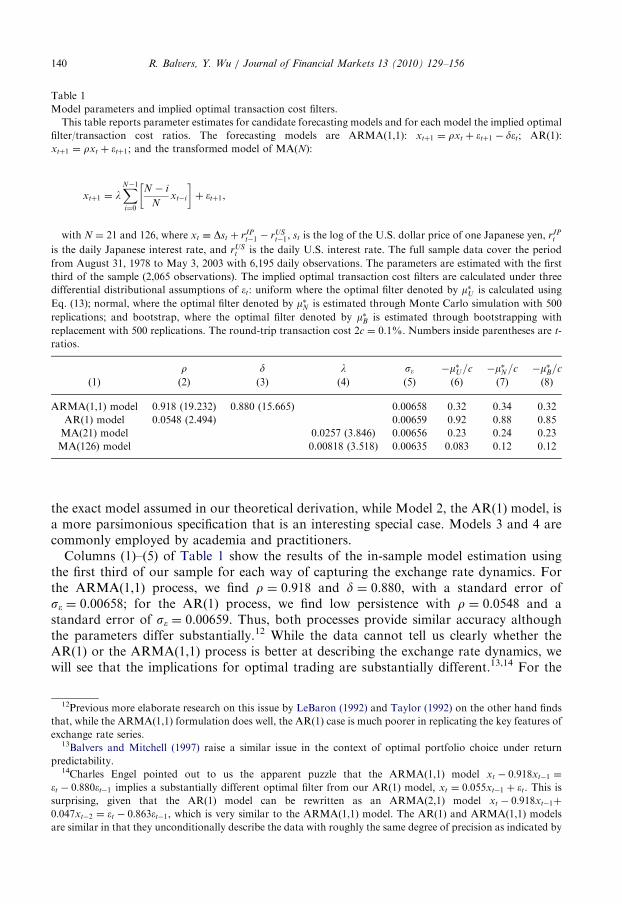
Table 1

Model parameters and implied optimal transaction cost filters.

This table reports parameter estimates for candidate forecasting models and for each model the implied optimal

filter/transaction cost ratios. The forecasting models are ARMA(1,1): xtþ1 ¼ rxt þ �tþ1 � d�t; AR(1):

xtþ1 ¼ rxt þ �tþ1; and the transformed model of MA(N):

xtþ1 ¼ lXN�1i¼0

N � i

Nxt�i

� �þ �tþ1,

with N ¼ 21 and 126, where xt � Dst þ rJPt�1 � rUS

t�1, st is the log of the U.S. dollar price of one Japanese yen, rJPt

is the daily Japanese interest rate, and rUSt is the daily U.S. interest rate. The full sample data cover the period

from August 31, 1978 to May 3, 2003 with 6,195 daily observations. The parameters are estimated with the first

third of the sample (2,065 observations). The implied optimal transaction cost filters are calculated under three

differential distributional assumptions of �t: uniform where the optimal filter denoted by m�U is calculated using

Eq. (13); normal, where the optimal filter denoted by m�N is estimated through Monte Carlo simulation with 500

replications; and bootstrap, where the optimal filter denoted by m�B is estimated through bootstrapping with

replacement with 500 replications. The round-trip transaction cost 2c ¼ 0.1%. Numbers inside parentheses are t-

ratios.

r d l s� �m�U=c �m�N=c �m�B=c

(1) (2) (3) (4) (5) (6) (7) (8)

ARMA(1,1) model 0.918 (19.232) 0.880 (15.665) 0.00658 0.32 0.34 0.32

AR(1) model 0.0548 (2.494) 0.00659 0.92 0.88 0.85

MA(21) model 0.0257 (3.846) 0.00656 0.23 0.24 0.23

MA(126) model 0.00818 (3.518) 0.00635 0.083 0.12 0.12

R. Balvers, Y. Wu / Journal of Financial Markets 13 (2010) 129–156140

the exact model assumed in our theoretical derivation, while Model 2, the AR(1) model, isa more parsimonious specification that is an interesting special case. Models 3 and 4 arecommonly employed by academia and practitioners.Columns (1)–(5) of Table 1 show the results of the in-sample model estimation using

the first third of our sample for each way of capturing the exchange rate dynamics. Forthe ARMA(1,1) process, we find r ¼ 0.918 and d ¼ 0.880, with a standard error ofse ¼ 0.00658; for the AR(1) process, we find low persistence with r ¼ 0.0548 and astandard error of se ¼ 0.00659. Thus, both processes provide similar accuracy althoughthe parameters differ substantially.12 While the data cannot tell us clearly whether theAR(1) or the ARMA(1,1) process is better at describing the exchange rate dynamics, wewill see that the implications for optimal trading are substantially different.13,14 For the

12Previous more elaborate research on this issue by LeBaron (1992) and Taylor (1992) on the other hand finds

that, while the ARMA(1,1) formulation does well, the AR(1) case is much poorer in replicating the key features of

exchange rate series.13Balvers and Mitchell (1997) raise a similar issue in the context of optimal portfolio choice under return

predictability.14Charles Engel pointed out to us the apparent puzzle that the ARMA(1,1) model xt � 0:918xt�1 ¼

�t � 0:880�t�1 implies a substantially different optimal filter from our AR(1) model, xt ¼ 0:055xt�1 þ �t. This issurprising, given that the AR(1) model can be rewritten as an ARMA(2,1) model xt � 0:918xt�1þ

0:047xt�2 ¼ �t � 0:863�t�1, which is very similar to the ARMA(1,1) model. The AR(1) and ARMA(1,1) models

are similar in that they unconditionally describe the data with roughly the same degree of precision as indicated by


representative moving average rule with 21 lags, we find for the slope in Eq. (16) thatl ¼ 0.0257 and se ¼ 0.00656. Since we have N ¼ 21, we obtain from Eq. (18) thatr ¼ 0.979 and d ¼ 0.954, which is not statistically distinguishable from the direct estimatesfrom the ARMA(1,1) model. The MA(126) process yields l ¼ 0.00818 and se ¼ 0.00635,implying by approximation that r ¼ 0.999 and d ¼ 0.992.

We assume one round trip transaction cost of 2c ¼ 0.001 (10 basis points) per switchthroughout.15 Sweeney (1986) finds a transaction cost of 12.5 basis points for majorforeign exchange markets, but more recent work by Bessembinder (1994), Melvin and Tan(1996), and Cheung and Wong (2000) finds bid–ask spreads for major exchange ratesbetween 5 and 9 basis points. To account for transaction costs in addition to thoseimbedded in the bid–ask spread, related to broker fees and commissions and thelending–borrowing interest differential, we use 10 basis points as a realistic number forthe dollar–yen market. The daily U.S. interest rate is on average over the first third of thesample equal to 0.000439%. This average rate is used as a proxy for the discount rate r incomputing the optimal filter in Eq. (13).

The true distribution of the exchange rate can be quite complex, and we do not know apriori which distributional assumption is the best approximation. Therefore we choose toestimate the optimal filter m� using three methods. First, under the assumption that theerror term et is uniformly distributed, the optimal filter, denoted m�U , can be analyticallycalculated using Eq. (13). Second, �t is assumed to follow a normal distribution. In thiscase, the result in Eq. (13) no longer holds, and we estimate the optimal filter, denoted m�N ,through Monte Carlo simulation. Last, we do not make an assumption about thedistribution of et and estimate the optimal filter, denoted m�B, by bootstrapping the modelresiduals �̂t with replacement.

3.3. The optimal filter implied by the theory under the uniform distribution

Under the assumption of a uniform distribution, we can obtain z from the relationz ¼

ffiffiffi3p

s�. All the information now is there to allow us to calculate the optimal filter fromEq. (13) for the dollar–yen exchange rate. Column (6) of Table 1 provides the results. Forthe AR(1) case, we find that the ratio of the critical return to the transaction cost is�m�U=c ¼ 0:92.16 Hence, in this case the optimal filter is not very different from a naı̈vefilter that equals the transaction cost c. The main reason is that, from Eq. (4), the

(footnote continued)

se in our Table 1. The reason they imply quite different filters is because the optimal filter depends on the

persistence of the conditional expected return. Eq. (4) says that the conditional expected return is an

AR(1) process, which becomes mt ¼ 0:918mt�1 þ ð0:918� 0:880Þ�t�1 ¼ 0:918mt�1 þ 0:038�t�1 for our empirical

ARMA(1,1) model, while our empirical AR(1) model (or the equivalent ARMA(2,1)) implies mt ¼ 0:055mt�1þ

0:055�t�1. We can see that the conditional expected return from the ARMA(1,1) model is much more persistent

than that from the AR(1) model. Therefore, we apply a smaller filter for the ARMA(1,1) model since even a small

positive expected one-period return is enough to make up for the transaction cost because the new position is

likely to remain optimal for a number of future periods.15Note that c in the model represents the cost of closing out a zero-investment position. For most assets this

requires both a sale and a purchase implying a round trip transaction cost. However, in the case of foreign

exchange, we directly purchase one currency with the other, implying only a one-way transaction cost. Reversing

the position requires double that transaction cost 2c, which is one round trip.16This ratio is the immediate gain of switching to �m� from m� (the gain of �2m�) divided by the transaction

cost 2c.


persistence in the mean return is small at r ¼ 0.0548 so that, no matter what the currentholdings are, there is not much difference in future probabilities of trading.For the 1-month MA process, the parameters backed out from the MA(21) model yield�m�U=c ¼ 0:23. Note that inequality (12) is violated, as is necessary here when�m�U=co0:50, implying that the analytical value obtained from Eq. (13) is no longeraccurate and must be viewed as a good approximation; hence, it is more precise to statethat �m�U=c 0:23. Intuitively, the slow adjustment in the conditional mean for theseparameter values implies that, in some cases, even the most extreme realization of theexchange rate innovation would not be sufficient to induce switching. Hence, one would becertain of avoiding transaction costs for at least one period (and likely more) by buying/keeping the exchange with the positive expected return. This explains the low value of thecritical expected return relative to the transaction cost.The 6-month MA process, MA(126), yields the smallest filter, �m�U=c ¼ 0:083. One

reason is the high persistence of expected return (the implied persistence parameterr ¼ 0.999). Another is the fact that by nature the long MA process is very smooth sochanges in the mean occur very slowly so that the number of transactions is small, evenwhen there is no filter. This is a possible reason for the popularity of this particular tradingrule with practitioners.For our main specification, the ARMA(1,1) case with r ¼ 0.918 and d ¼ 0.880, we

find that the optimal filter is �m�U=c ¼ 0:32. The reason that this number is so much lowerthan under the AR(1) case is clear from Eq. (4). The persistence is not only high nowwith r ¼ 0.918 but it is also high relative to the innovation in the conditional mean,given by ðr� dÞs� ¼ 0:038s�. Hence, it is highly likely that the exchange position (dollar oryen) with the currently positive expected return is going to be unchanged in the nearbyfuture.

3.4. The optimal filter obtained numerically

As a check on the dependence of the results on the uniform distribution, we also find theoptimal filter numerically using a Monte Carlo approach, assuming normality and abootstrapping approach.For each Monte Carlo trial, we simulate expected returns mt using Eq. (16) with

parameters estimated from the first third of the sample. We then choose the filter m�N , whichmaximizes the after-cost average excess return. This process is replicated 500 times.Column (7) of Table 1 reports the median value of the optimal filter to transaction costratio, �m�N=c, over the 500 Monte Carlo trials. For each model, the ratio �m�N=c is quiteclose to the optimal ratio implied under the uniform distribution, �m�U=c, with thedifference between them never exceeding 5% of the transaction cost.The actual distribution of �t may be neither uniform nor normal. In this case, we re-

sample with replacement the fitted residuals �̂t of Eq. (16) and use model parameters togenerate expected return observations mt. Similar to the Monte Carlo experiment, for eachbootstrapping trial, the optimal filter is chosen to be the one that maximizes the after-costaverage excess return. Column (8) of Table 1 reports the median estimate of the optimalfilter to cost ratio �m�B=c over 500 bootstrapping replications. Encouragingly, the optimalfilters, for the theoretical uniform distribution case and the numerical normal andbootstrapping cases, are quite similar for each of the returns processes. Thus, the optimalfilter value is robust to distributional assumptions.


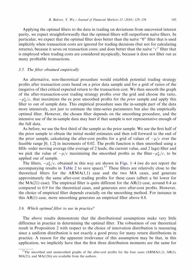
Applying the optimal filters to the data in trading on deviations from uncovered interestparity, we expect straightforwardly that the optimal filters will outperform naı̈ve filters. Inparticular, we expect that the optimal filter does better than the naı̈ve ‘‘0’’ filter that is usedimplicitly when transaction costs are ignored for trading decisions (but not for calculatingreturns), because it saves on transaction costs; and does better than the naı̈ve ‘‘c’’ filter thatis employed when trading costs are considered myopically, because it does not filter out asmany profitable transactions.

3.5. The filter obtained empirically

An alternative, non-theoretical procedure would establish potential trading strategyprofits after transaction costs based on a prior data sample and for a grid of ratios of the(negative of the) critical expected return to the transaction cost. We then smooth the graphof the after-transaction-cost trading strategy profits over the grid and choose the ratio,�m�E=c, that maximizes the ex post smoothed profits for the prior sample and apply thisfilter to out of sample data. This empirical procedure uses the in-sample part of the datamore intensively, not just to estimate the time-series parameters but also the empiricallyoptimal filter. However, the chosen filter depends on the smoothing procedure, and theintensive use of the in-sample data may hurt if that sample is not representative enough ofthe full data.

As before, we use the first third of the sample as the prior sample. We use the first half ofthe prior sample to obtain the initial model estimates and then roll forward to the end ofthe prior sample, calculating the after-cost profits for a grid of values of �m=c over thefeasible range [0, 1.2] in increments of 0.02. The profit function is then smoothed using afifth- order moving average (the average of 2 leads, the current value, and 2 lags) filter andwe pick the value of �m=c maximizing the smoothed profits as the filter�m�E=c, to beapplied out of sample.

The filters, �m�E=c, obtained in this way are shown in Figs. 1–4 (we do not report theaccompanying results in Table 2 to save space).17 These filters are relatively close to thetheoretical filters for the ARMA(1,1) case and the two MA cases, and generateapproximately the same after-cost trading profits for these cases (albeit a bit lower forthe MA(21) case). The empirical filter is quite different for the AR(1) case, around 0.4 ascompared to 0.9 for the theoretical cases, and generates zero after-cost profits. However,the choice of empirical filter depends crucially on the smoothing method. For instance inthis AR(1) case, more smoothing generates an empirical filter above 0.8.

3.6. Which optimal filter to use in practice?

The above results demonstrate that the distributional assumptions make very littledifference in practice in determining the optimal filter. The robustness of our theoreticalresult in Proposition 2 with respect to the choice of innovation distribution is reassuringsince a uniform distribution is not exactly a good proxy for many return distributions inpractice. A reason for the apparent irrelevance of this assumption may be that, in thisapplication, we implicitly have that the first three distribution moments are the same for

17The smoothed and unsmoothed graphs of the after-cost profits for the four cases (ARMA(1,1), AR(1),

MA(21), and MA(126)) are available from the authors.

ARTICLE IN PRESS

Fig. 1. The effect of filter on after-cost returns for the ARMA(1,1) model. Note: The solid line with round

symbols displays the after-cost excess return and the one with square symbols displays the trading cost. The

vertical lines represent different filters: the solid line is the theoretical optimal filter under uniform distribution

�m�U=c; the short dashed line is the optimal filter under normal distribution �m�N=c; the long dashed line is the

optimal filter under bootstrap distribution �m�B=c; and the dotted line is the ad hoc filter that maximizes the in-

sample smoothed after-cost excess return using the first third of the sample, �m�E=c.


any innovation distribution. This occurs because the mean of the distribution is set to zeroin each case, the variance is calibrated to be the same in each case, and the skewness issimilar in each case because of the symmetry in the returns of zero-investment positionsrelative to their reverse.The effective similarity of different return distributions in this case together with the

obtained similarity in the results in Table 2 for the different distributions both argue forusing Proposition 2, which holds for the uniform distribution only, in practice. Calculationof the optimal filter can be performed directly from Eq. (13) and does not requiresimulations. Given the transaction cost and riskless interest rate, only a prior estimate ofthe ARMA(1,1) process is needed, yielding the autoregressive parameter, r, the movingaverage parameter, d, and the estimate of the innovation variance, s2� (the latterdetermining z from z ¼ 31=2s�). Note also that the alternative models, the AR(1) and theMA models, are simply special cases of our model that we have employed to illustrate theimplications of particular trading rules often used in foreign exchange markets. Based alsoon the results of LeBaron (1992) and Taylor (1992), who find that this specification ispreferred with data prior to our holdout sample, it should be clear that the ARMA(1,1)process assumed in the theoretical model is the preferred specification for application.Accordingly, for given prior and holdout samples, the optimal filter can be obtained simplyand uniquely.

ARTICLE IN PRESS

Fig. 2. The effect of filter on after-cost returns for the AR(1) model. Note: The solid line with round symbols

displays the after-cost excess return and the one with square symbols displays the trading cost. The vertical lines

represent different filters: the solid line is the theoretical optimal filter under uniform distribution �m�U=c; the short

dashed line is the optimal filter under normal distribution �m�N=c; the long dashed line is the optimal filter under

bootstrap distribution �m�B=c; and the dotted line is the ad hoc filter that maximizes the in-sample smoothed after-

cost excess return using the first third of the sample, �m�E=c.

R. Balvers, Y. Wu / Journal of Financial Markets 13 (2010) 129–156 145

4. Out-of-sample optimal switching strategy results

4.1. Description of the strategy

We start our first-day forecast on November 28, 1986 (after the first third of thesample).18 For each of the four exchange rate return specifications, we estimate the modelparameters using all observations for the first third of the sample (up to November 27,1986) and make the first forecast (for November 28). If the forecasted return (recall thatthe return is defined as the difference between the return from holding the Japanese yen,which is the percentage exchange rate change plus the one-day Japanese interest rate, andthe return from holding the U.S. dollar, which is the one-day U.S. interest rate) is positive,we take a long position in the yen, and simultaneously take a short position in the dollar.Conversely, if the forecasted return is negative, we take a long position in the dollar and ashort position in the yen. The difference in returns between the long and short positionsrepresents the return from a zero-cost investment strategy. While daily data are employedin this study, bid–ask bounce is not an issue here since the exchange rate data give the lastobservation on the midpoint of the bid and ask prices; further, due to the heavy trading

18Our results appear to be quite robust to the starting point of the forecast period: results for each of the four

models are very similar if we start the forecast period at 14or 1

2of the sample instead of at 1

3.

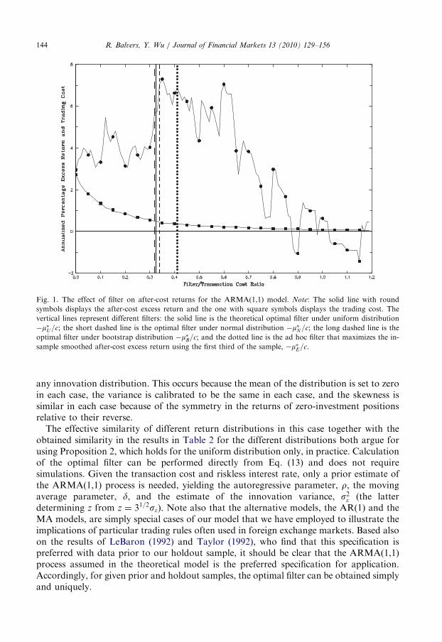
ARTICLE IN PRESS

Fig. 3. The effect of filter on after-cost returns for the MA(21) model. Note: The solid line with round symbols

displays the after-cost excess return and the one with square symbols displays the trading cost. The vertical lines

represent different filters: the solid line is the theoretical optimal filter under uniform distribution�m�U=c; the short

dashed line is the optimal filter under normal distribution �m�N=c; the long dashed line is the optimal filter under

bootstrap distribution �m�B=c; and the dotted line is the ad hoc filter that maximizes the in-sample smoothed after-

cost excess return using the first third of the sample, �m�E=c.


volume of the yen, non-synchronous trading issue is not relevant. Additionally, while thedaily interest observations do not coincide exactly with the exchange rate observations, thehigh volatility of the exchange rate relative to the interest rates implies that any bias due toa timing mismatch is probably negligible.From the second forecasted day (November 29) until the end of the sample, our strategy

works as follows. For each day, we use all available observations to estimate the modelparameters and forecast the excess return for the following day. If either of the followingtwo conditions occurs, a transaction will take place. (1) If the forecasted excess return ispositive, its magnitude is larger than the transaction cost filter, and we currently have along position in the dollar (and a short position in the yen), then we reverse our position bytaking a long position in the yen and a short position in the dollar for the following day.This counts as one trade involving two one-way transaction costs. (2) If the forecastedexcess return is negative, its magnitude is larger than the transaction cost filter, and thecurrent holdings are long in the yen and short in the dollar, then we reverse our position bytaking a long position in the dollar and a short position in the yen. This counts as onetransaction and again involves two one-way transaction costs. If neither of the above twoconditions applies, no trade takes place. The current holdings (both long and short) carryover to the following day and no transaction costs are incurred.We compute the average excess return for the zero-cost investment strategy and the

associated t-ratio for the out-of-sample forecasting period. We document the before-cost

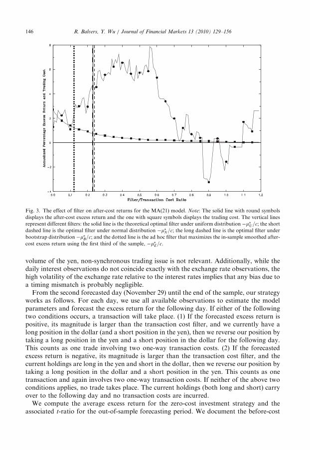
ARTICLE IN PRESS

Fig. 4. The effect of the filter on after-cost returns for the MA(126) model. Note: The solid line with round

symbols displays the after-cost excess return and the one with square symbols displays the trading cost. The

vertical lines represent different filters: the solid line is the theoretical optimal filter under uniform distribution

�m�U=c; the short dashed line is the optimal filter under normal distribution �m�N=c; the long dashed line is the

optimal filter under bootstrap distribution �m�B=c; and the dotted line is the ad hoc filter that maximizes the in-

sample smoothed after-cost excess return using the first third of the sample �m�E=c.

R. Balvers, Y. Wu / Journal of Financial Markets 13 (2010) 129–156 147

and after-cost excess return rates for the case without filter, and the after-cost excess returnrates for the cases with transaction cost filter. For perspective, the simple buy-and-holdstrategy of holding the yen and shorting the dollar over the whole out-of-sample periodyields an annualized return of �0.00953 (the reverse strategy of holding the dollar andshorting the yen yields therefore +0.00953), o1%. This return is not statisticallydistinguishable from zero (t-ratio ¼ 0.348).

4.2. Basic results

Table 2 reports the results for the four forecasting models. Each model is discussedseparately below. For the ARMA(1,1) model, the before-cost excess return in the casewithout a filter is 5.7% per annum, which is statistically significant at the 5% level. Thestrategy, however, requires 444 trades over 4,130 trading days and accounting for theround-trip costs of 10 basis points reduces the after-cost excess return to 3.0%, which is nolonger statistically significant. The naı̈ve filter equal to the 5 basis points one-waytransaction cost ‘‘c’’ dramatically reduces the number of trades to 12, resulting in a lowerexcess return of 0.6%, which is statistically insignificant. In contrast, the optimal filter, m�U ,captures many of the profitable trades and yields an excess return of 5.5%, which issignificant at the 5% level. The filter under the bootstrapped distribution m�B produces

ARTIC

LEIN

PRES

S

Table 2

Effects of transaction costs on trading performance in foreign exchange.

This table reports trading performance in the Japanese yen with a round-trip transaction cost 2c ¼ 0.1%. The data cover the period from August 31, 1978 to May

3, 2003 with 6,195 daily observations. The first third of the sample (2,065 observations) is used for model estimation. The parameter estimates are used to calculate the

optimal transaction cost filters. Out-of-sample forecasting starts on November 28, 1986 until the end of the sample (4,130 observations). Columns 1–5 display results

where no transaction cost filter is imposed. Columns 2–3 report the before-cost excess returns (from the zero-cost investment strategies) and t-ratios, whereas Columns

4–5 report the after-cost excess returns and t-ratios. Similarly, Columns 6–8 report the results (after-cost) when a naı̈ve filter equal to the actual transaction cost c is

imposed. Columns 9–11, 12–14, and 15–17, show the results when the optimal filters, m�U , m�N and m�B, are imposed, respectively. All returns are annualized.

Model Without transaction cost filter With naı̈ve filter ‘‘c’’ With optimal filter m�U With optimal filter m�N With optimal filter m�B

Before cost After cost After cost After cost After cost After cost

# of

trades

Excess

return

t-

Ratio

Excess

return

t-ratio # of

trades

Excess

return

t-

Ratio

# of

trades

Excess

return

t-

Ratio

# of

trades

Excess

return

t-

Ratio

# of

trades

Excess

return

t-

Ratio

(1) (2) (3) (4) (5) (6) (7) (8) (9) (10) (11) (12) (13) (14) (15) (16) (17)

ARMA(1,1) 444 0.057 2.054 0.030 1.073 12 0.006 0.225 81 0.055 2.007 71 0.070 2.549 81 0.057 2.050

AR(1) 2100 0.069 2.486 �0.059 �2.144 34 0.011 0.390 42 0.058 2.105 48 0.056 2.017 66 0.026 0.940

MA(21) 448 0.040 1.453 0.013 0.463 12 �0.015 �0.560 125 0.044 1.591 123 0.044 1.596 125 0.048 1.728

MA(126) 131 0.065 2.338 0.057 2.047 5 �0.020 �0.714 31 0.059 2.143 29 0.047 1.715 29 0.047 1.715

R.

Ba

lvers,Y

.W

u/

Jo

urn

al

of

Fin

an

cial

Ma

rkets

13

(2

01

0)

12

9–

15

6148


nearly the same results as m�U , whereas the filter under the normality assumption, m�N , yieldsan even higher return of 7.0%, which is significant at the 1% level.

For the AR(1) model, the strategy without filter involves 2,100 switches over 4,130trading days (over 50% of the time). In the absence of transaction costs, the strategyproduces an annualized excess return of 6.9% with a t-ratio of 2.486, which is statisticallysignificant at the 5% level. However, the transaction cost completely wipes out the profits,resulting in a negative excess return of 5.9%. A naı̈ve filter equal to the actual round-triptransaction cost of 10 basis points dramatically reduces the number of transactions to 34,and yields an insignificant excess return of 1.1% per annum. While it is somewhat useful,this naı̈ve filter may be too conservative because it does not exploit the information on thepersistence of expected return in the exchange rate, thereby missing a number of profitabletrades. The strategy with the optimal filter m�U under the assumption of a uniformdistribution captures just that opportunity. It produces 42 trades and yields a higher excessreturn of 5.8%, which is significant at the 5% level. Similarly, the optimal filter under thenormality assumption m�N produces an average excess return of 5.6% per annum, alsosignificant at the 5% level. The bootstrapped filter m�B yields an insignificant excess returnof 2.6%.

For the MA(21) model, our strategy with the optimal filters again generates higherexcess returns than the alternatives, although none of the excess returns are statisticallysignificant at the 5% level.

Finally, the long MA(126) process provides a very smooth forecast of expected returns.While the strategy without filter yields an after-cost return of 5.7 %, which is significant atthe 5% level, the naı̈ve filter equal to c skips too many profitable trades, resulting in anegative return of 2%. The optimal filter m�U , while very small relative to c, is capable offiltering many days with low expected returns and capturing those days when expectedreturns are substantial. This filter produces an expected return of 5.9%, which is significantat the 5% level. The other two filters, m�N and m�B, yield somewhat smaller returns (4.7%),which are statistically significant only at the 10% level.19

4.3. Filter size and after-cost excess returns

Figs. 1–4 display the trading strategy returns (after cost) and trading costs for the fourreturn processes as a function of the filter value. As expected, the trading cost declinesmonotonically as the filter value rises. The after-cost excess return lines illustrate that in allcases the ex ante optimal filters are reasonably close to the ex post optimum (with theempirical filter in the AR(1) case being the only exception). Since the actual data are justone random draw from the unobserved true process, this is all one should expect of a goodmodel. Except for the AR(1) case, the trading strategy returns display the hump-shapedpattern expected for the after-cost returns.

A striking feature of these four figures is that, even though the optimal filters differradically across the four cases, the empirical (ex post) maximum filter value is quite close tothe (ex ante) optimal filter in all four cases. While each case approximates the true dataprocess to a certain extent, it is not surprising that the ARMA(1,1) process provides the

19The trading strategies for each of the forecasting models imply a reasonably even choice of each currency. For

example, with the optimal filter m�U , the fraction of long yen and short U.S. dollar is: ARMA(1,1) 1830/4130,

AR(1) 2555/4130, MA(21) 1987/4130, and MA(216) 1875/4130.


best overall fit as it is well-known to be a parsimonious description of general ARMA(p, q)processes. The strong performance of the ARMA(1,1) process and the poorer performanceof the AR(1) process is consistent with the results of LeBaron (1992) and Taylor (1992)that ARMA(1,1) processes are far better at capturing the key features of exchange rateseries.20,21

4.4. Correction for potential data snooping

The previous subsections report the trading strategy results by examining multiplemodel specifications. Overall, we explore four data-generating processes (ARMA(1,1),AR(1), MA(21), and MA(126)) with three distributions (uniform, normal, and bootstrap),yielding a total of 12 different specifications. It would be undue and incorrect for aresearcher to report only the best-performing specification or draw inferences based solelyon the best-performing specification, as doing so leads to a so-called data-snooping bias.Traditionally, bounds on the p-value for tests of the null when multiple specifications are

investigated can be constructed using the Bonferroni inequality [see, for example,Lehmann and Modest, 1987 for an application]. White (2000) develops a novel procedure,called Reality Check, to measure and correct for data-snooping biases. The idea is togenerate the empirical distribution from the full set of specifications that generates thebest-performing outcome and to draw inferences from this distribution. We apply thismethodology to check for the robustness of our results.White’s (2000) test evaluates the distribution of a performance measure, accounting for

the full set of specifications that lead to the best-performing specification. In our case, theperformance measure is the after-cost excess return. The null hypothesis to be tested is thatthe best specification is no better than the benchmark (which is zero excess return), i.e.,

H0 : maxk¼1;...;L

fEðRkÞg � 0, (19)

where k denotes a specification, L is the total number of specifications, the expectation isevaluated with the average

R̄k ¼1

T

XT

t¼1

Rk;t.

Rk;t is the after-cost excess return of specification k at time t, and T is the number offorecasting periods. Rejection of the null will lead to the conclusion that the bestspecification achieves performance superior to the benchmark.Following White (2000), we test the null hypothesis H0 by applying the stationary

bootstrap method of Politis and Romano (1994) to the observed values of Rk;t as follows.

20Figures available from the authors provide a breakdown of the effect of the optimal filters on trading

frequency. In each of the models, the optimal filters, the m�U , reduce trading frequency considerably but the trades

remain quite evenly distributed over time. For instance, for the ARMA(1,1) model, a minimum of two trades and

a maximum of eight trades occurs in each (full) year under the optimal filter trading strategy.21A table available from the authors provides risk-adjusted trading rule returns. We correct the ex post trading

rule returns from each of the four forecast models for CAPM market risk using the MSCI World market index

and the euro interest rate as the risk-free rate (results using the U.S. S&P 500 value-weighted market index are

similar). In all cases the market risk sensitivities of the zero-cost investment positions are near zero. Thus, the risk-

adjusted returns, the ‘‘alphas,’’ are very close to the unadjusted returns.


Step 1: We resample the realized excess return series Rk;t, one block of observations at atime with replacement, and denote the resulting series by R�k;t. This process is repeated N

times.Step 2: For each replication i, we compute the sample average of the bootstrapped

returns, denoted by

R̄�

k;i �1

T

XT

t¼1

R�k;t; i ¼ 1; . . . ;N.

Step 3: We construct the following statistics:

V̄ ¼ maxk¼1;...;L

fffiffiffiffiTpðR̄kÞg, (20)

V̄�

i ¼ maxk¼1;...;L

fffiffiffiffiTpðR̄�

k;i � R̄kÞg; i ¼ 1; . . . ;N. (21)

Step 4: White’s Reality Check p-value is obtained by comparing V̄ to the percentilesof V̄

�

i .Our out-of-sample forecasting period contains 4,130 observations, and we experiment

with a total of 12 specifications; therefore, T ¼ 4,130 and L ¼ 12. We choose N ¼ 10; 000.With the smoothing parameter set equal to 0.5,22 we find a White p-value of 0.034. Ourresults are robust to the value of the smoothing parameter. We obtain White p-values of0.041, 0.030, and 0.032, for smoothing parameter values of 0.1, 0.9, and 1, respectively.These results imply that the null hypothesis that our trading strategy does not produce anafter-cost excess return can be rejected at the 5% significance level even after properlyaccounting for the potential data-snooping bias. The robustness of these results should,however, be interpreted with caution because our Reality Check simulation for data-snooping bias correction is based on the 12 trading rules experimented with in this paperbut does not account for all the rules studied in the literature.

5. Conclusion

If transitory profitable trading opportunities exist, transaction filters are used inpractice to mitigate trading costs; but the filter size is difficult to determine a priori.This paper uses a dynamic programming framework to design a filter that is optimal inthe sense of maximizing expected returns after transaction costs. The optimal filtersize depends negatively on the degree of persistence of the profitable trading opportuni-ties, positively on transaction costs, and positively on the standard deviation ofshocks.

We apply our theoretical results to foreign exchange trading by parameterizing themoving average strategy often employed in foreign exchange markets. The parameteriza-tion implies the same decisions as the moving average rule in the absence of transactioncosts, but has the advantage of translating the buy/sell signal into the same units as thetransaction costs so that the optimal filter can be calculated.

22The smoothing parameter, which is greater than 0 and no greater than 1, controls the block length in the

bootstrap re-sampling. A larger value is appropriate for data with little dependence and a smaller value is

appropriate for data with more dependence [see Politis and Romano, 1994; White, 2000].


Application to daily dollar–yen trading demonstrates that the optimal filter is not solelyof academic interest but may differ to an economically significant extent from a naı̈ve filterequal to the transaction cost. This depends importantly on the time series process that weassume for the exchange rate dynamics. In particular, we find that for an AR(1) process,the optimal filter is close to the naı̈ve transaction cost filter, but for the ARMA(1,1)process, the optimal filter is only around 30% of the naı̈ve transaction cost filter, and forthe more stable MA processes, the optimal filter is smaller still as a fraction of thetransaction cost. Impressively, the ex ante optimal filters under the assumptions ofuniform, normal, and bootstrap distributions are all very close to one another and all arequite close to the ex post after-cost return-maximizing level.We confirm that simple daily moving average foreign exchange trading generates

positive returns that disappear after accounting for transaction costs. However, when theoptimal filter is used, returns after transaction costs remain positive and are higher than fornaı̈ve filters. This result has implications beyond foreign exchange markets. It cautionsagainst dismissing abnormal returns as due to transactions costs, merely because the after-cost return is negative or insignificant. For instance, Lesmond et al. (2004) argueconvincingly that momentum profits disappear when actual transaction costs are properlyconsidered, even after accounting for the proportion of securities held over in each period.But their after-cost returns are akin to those for our suboptimal zero filter strategy. Itwould be interesting to see what outcome would arise if an optimal filter were used.In our sample, the trading strategy returns, gross of transaction costs, are significantly

positive, but no longer significant after transaction costs are subtracted. But if weoptimally eliminate trades that do not make up for their transaction cost, then the after-cost profits are only slightly lower than the gross profits from unrestricted trading and arestatistically significant. They are also economically significant, around 0.5% per monthafter transaction costs, which raises the issue of market efficiency. The profits are of similarmagnitude as the momentum profits after transaction costs and may in fact be closelyrelated to the momentum phenomenon. However, given the lower total variance of thetrading strategy returns,23 it is even more difficult here, compared to the momentum casefor equity returns, to argue that an unobserved systematic risk is responsible. So the‘‘anomaly’’ may be exploitable and, in the absence of a risk explanation, could suggestmarket inefficiency.Apart from the practical advantages of using the optimal filter, there is also a

methodological advantage: in studies attempting to calculate abnormal returns fromparticular trading strategies in which transaction costs are important, there is no guidelineas to what filter to use in dealing with transaction costs. Lesmond et al. (2004, p. 370) note:‘‘Although we observe that trading costs are of similar magnitude to the relative strengthreturns for the specific strategies we consider, there is an infinite number of momentum-oriented strategies to evaluate, so we cannot reject the existence of trading profits for allstrategies’’. Rather than allowing the data-mining problem that is likely to arise when avariety of filter sizes are applied, our approach here provides a unique filter in Eq. (13) thatcan be unambiguously obtained in advance from observable variables.

23For example, from Jegadeesh and Titman (1993), the standard deviation of momentum excess return for the

6-month sorting and 6-month holding strategy is 5.4% per month. Based on our theoretical optimal filter, m�U , thestandard deviation of after-cost return for the ARMA(1,1) specification is 0.7% per day, or 3.2% per month,

which is lower than that from the momentum strategy.


Acknowledgments

We would like to thank Gershon Alperovich, Ake Blomqvist, Ivan Brick, Justin Chan,Sris Chatterjee, N.K. Chidambaran, Chong Tze Chua, Charles Engel, Aditya Goenka,Sam Henkel, Dong Hong, Lixin Huang, Qiang Kang, James Lothian, Paul McNelis, SalihNeftci, Darius Palia, Andrew Rose, Menahem Spiegel, John Wald, Yonggan Zhao, theeditor (Bruce Lehmann), the anonymous referee, and seminar participants at the FinancialManagement Association International, the Pacific Basin Finance, Economics andAccounting Conference, the China International Conference in Finance, FordhamUniversity, Nanyang Technological University, the National University of Singapore,Peking University, Rutgers University, Singapore Management University and theUniversity of Hong Kong for helpful conversations and comments. Yangru Wu wouldlike to thank the Whitcomb Center at the Rutgers Business School and the Office ofResearch of Singapore Management University for financial support. Part of this workwas completed while Yangru Wu visited Singapore Management University and theCentral University of Finance and Economics. He would like to thank these institutionsfor their hospitality. We are solely responsible for any remaining errors.

Appendix A

A.1. Proof of Proposition 1

In Eq. (1), consider that V2ðxt�1; �t�1Þ ¼ V 1ð�xt�1;��t�1Þ by virtue of the fact that, forthe symmetric distribution of innovations, the expected returns of one position areequivalent to the expected returns of the reverse position if the return variables in Eq. (2)are the negative. Define mt � Et�1xt. Then, given Eq. (2), we have mtþ1 � rxt � d�tand thus we can without loss of generality redefine the state variables so thatV 1ðxt; �tÞ � V ðmtþ1; �tÞ. Then Eq. (1) becomes:

V ðmt; �t�1Þ ¼ mt þ Et�1 MaxV ðmtþ1; �tÞ

1þ r;V ð�mtþ1;��tÞ

1þ r� 2c

� �� . (A.1)

To derive Eq. (4), consider Eq. (2), xt � rxt�1 ¼ �t � d�t�1. Taking conditionalexpectations on both sides yields xt � rxt�1 � d�t�1. Now lag the first equation by oneperiod and take conditional expectations at time t�2. Simple algebra yieldsxt�1 ¼ mt�1 þ �t�1. Combining the last two equations produces Eq. (4), which says thatthe conditional expected return of the ARMA(1,1) model is an AR(1) process. It is furtherclear, by inspection of the decision problem now summarized by Eqs. (A.1) and (4), that,once the state variable mt is considered, there is no additional role for the state variable�t�1. Thus, we obtain V ðmt; �t�1Þ � V ðmtÞ and (A.1) becomes:

V ðmtÞ ¼ mt þ Et�1 MaxV ðmtþ1Þ

1þ r;V ð�mtþ1Þ

1þ r� 2c

� �� . (A.2)

By the symmetry of the density function, we also have

V ð�mtÞ ¼ �mt þ Et�1 MaxV ð�mtþ1Þ

1þ r;V ðmtþ1Þ

1þ r� 2c

� �� . (A.20)


From (A.2) and (A.20), we have

V ð�mtÞ � V ðmtÞ

¼ �2mt þ

Zf�t:�2c�ðV�mtþ1Þ�ðV ðmtþ1ÞÞ=ð1þrÞ�2cg


1þ rdF ð�tÞ

þ 2c

Zf�t:ðV ð�mtþ1Þ�V ðmtþ1ÞÞ=ð1þrÞ42cg

dF ð�tÞ �

Zf�t:�2c4ðV ð�mtþ1Þ�V ðmtþ1ÞÞ=ð1þrÞg

dF ð�tÞ

" #,

(A.3)

which evaluates the Max contingent on the possible realizations of the innovation et. It canbe shown by induction that V ð�mtÞ � V ðmtÞ is strictly decreasing in mt (it is true for someterminal time T; then, if it holds for some time t+1, and given that r40 in Eq. (4), thesecond term on the right-hand side of (A.3) is also decreasing in mt and we can establish theresult for time t. Then let T go to infinity). Further, a unit decrease in mt increases V ð�mtÞ �

V ðmtÞ by at least 2 (the direct gain from switching). Hence, since the innovation et hasunbounded support, then the distribution of mtþ1 is unbounded and there exists exactly onefinite value m� at which ðV ð�m�Þ � V ðm�ÞÞ=ð1þ rÞ ¼ 2c. Accordingly, the investormaintains the current zero-investment position whenever mtþ14m� and reverses thecurrent position whenever mtþ1 � m�. It is then straightforward to convert (A.2) to Eq. (3).

A.2. Derivation of Eq. (5)

From Eq. (3), V ð�mtÞ is given as

V ð�mtÞ ¼ � mt þ

Z 1ðm�þrmtÞ=ðr�dÞ

V ½�rmt þ ðr� dÞ�t�

1þ r

� �dF ð�tÞ

þ

Z ðm�þrmtÞ=ðr�dÞ

�1

V ½rmt � ðr� dÞ�t�

1þ r� 2c

� �dF ð�tÞ. (A.4)

Using the symmetry property of the density function and a change in variable from et to�et, we can write Eq. (A.4) as follows:

V ð�mtÞ ¼ �mt þ


�1

V ð�mtþ1Þ

1þ r

� �dF ð�tÞ þ

Z 1ð�m��rmtÞ=ðr�dÞ

V ðmtþ1Þ

1þ r� 2c

� �dF ð�tÞ.

(A.5)

Then, from Eqs. (3) and (A.5), we obtain

V ð�mtÞ � V ðmtÞ ¼ �2mt þ BðmtÞ þ CðmtÞ,

with

BðmtÞ ¼




1þ r

� �dF ð�tÞ, (A.6)

CðmtÞ ¼ �2c

Z 1ð�m��rmtÞ=ðr�dtÞ

dF ð�tÞ �


�1

dF ð�tÞ

!¼ 2c


ðm�þrmtÞ=ðr�dÞdF ð�tÞ,

(A7)


where the last equality follows from the symmetry of the density function. Thus,

V ð�mtÞ � V ðmtÞ ¼ � 2mt þ




1þ r

� �dF ð�tÞ

þ 2c


ðm�þrmtÞ=ðr�dÞdF ð�tÞ, (A.8)

which is Eq. (5) given the definitions in Eqs. (6) and (7).

References

Alexander, S.S., 1961. Price movements in speculative markets: trends or random walks. Industrial Management

Review 2, 7–26.

Balduzzi, P., Lynch, A.W., 1999. Transaction costs and predictability: some utility cost calculations. Journal of

Financial Economics 52, 47–78.

Balvers, R.J., Mitchell, D.W., 1997. Autocorrelated returns and optimal intertemporal portfolio choice.

Management Science 43, 1537–1551.

Balvers, R.J., Wu, Y., Gilliland, E., 2000. Mean reversion across national stock markets and parametric

contrarian investment strategies. Journal of Finance 55, 745–772.

Bessembinder, H., 1994. Bid–ask spreads in the interbank foreign exchange markets. Journal of Financial

Economics 35, 317–348.

Canova, F., 1991. An empirical analysis of ex ante profits from forward speculation in foreign exchange markets.

Review of Economics and Statistics 73, 489–496.

Cheung, Y.W., Wong, C., 2000. A survey of market practitioners’ view on exchange rate dynamics. Journal of

International Economics 51, 401–419.

Cooper, M., 1999. Filter rules based on price and volume in individual security overreaction. Review of Financial

Studies 12, 901–935.

Cornell, W.B., Dietrich, J.K., 1978. The efficiency of the market for foreign exchange under floating exchange

rates. Review of Economics and Statistics 60, 111–120.

Engel, C., 1996. The forward discount anomaly and the risk premium: a survey of recent evidence. Journal of

Empirical Finance 3, 123–191.

Fama, E.F., Blume, M., 1966. Filter rules and stock market trading profits. Journal of Business 39, 226–241.

Frankel, J.A., Froot, K.A., 1990. Chartists, fundamentalists, and trading in the foreign exchange market.

American Economic Review 80, 181–185.

Gencay, R., 1999. Linear, nonlinear and essential foreign exchange prediction with simple technical rules. Journal

of International Economics 47, 91–107.

Gencay, R., Ballocchi, G., Dacorogna, M., Olsen, R., Pictet, O., 2002. Real-time trading models and the statistical

properties of foreign exchange rates. International Economic Review 43, 463–491.

Grundy, B., Martin, J.S., 2001. Understanding the nature and the risks and the sources of the rewards to

momentum investing. Review of Financial Studies 14, 29–78.

Hanna, J.D., Ready, M.J., 2005. Profitable predictability in the cross-section of stock returns. Journal of

Financial Economics 78, 463–505.

Jegadeesh, N., Titman, S., 1993. Returns to buying winners and selling losers: implications for stock market

efficiency. Journal of Finance 48, 65–91.

Knez, P.J., Ready, M.J., 1996. Estimating the profits from trading strategies. Review of Financial Studies 9,

1121–1163.

LeBaron, B., 1992, Do moving average trading rule results imply nonlinearities in foreign exchange markets?

Technical Report, University of Wisconsin–Madison.

LeBaron, B., 1998. Technical trading rules and regime shifts in foreign exchange. In: Acar, F., Satchell, S. (Eds.),

Advanced Trading Rules. Butterworth-Heinemann, Woburn, MA, pp. 5–40.

LeBaron, B., 1999. Technical trading rule profitability and foreign exchange intervention. Journal of International


Lee, C.I., Mathur, I., 1996. Trading rule profits in European currency spot cross rates. Journal of Banking and

Finance 20, 949–962.


Lehmann, B.N., 1990. Fads, martingales, and market efficiency. Quarterly Journal of Economics 105, 1–28.

Lehmann, B., Modest, D.M., 1987. Mutual fund performance evaluation: a comparison of benchmarks and

benchmark comparisons. Journal of Finance 42, 233–265.

Lesmond, D.A., Schill, M.J., Zhou, C., 2004. The illusory nature of momentum profits. Journal of Financial


Levich, R.M., Thomas, L.R., 1993. The significance of technical trading-rule profits in the foreign exchange

market: a bootstrap approach. Journal of International Money and Finance 12, 451–474.

Liu, H., 2004. Optimal consumption and investment with transaction costs and multiple risky assets. Journal of

Finance 59, 289–338.

Liu, H., Loewenstein, M., 2002. Optimal portfolio selection with transaction costs and finite horizons. Review of

Financial Studies 15, 805–835.

Lynch, A.W., Balduzzi, P., 2000. Predictability and transaction costs: the impact on rebalancing rules and

behavior. Journal of Finance 55, 2285–2310.

Lynch, A.W., Tan, S., 2009. Multiple risky assets, transaction costs and return predictability: allocation rules and

implications for US investors. Journal of Financial and Quantitative Analysis, forthcoming.

Mark, N.C., Wu, Y., 1998. Rethinking deviations from uncovered interest parity: the role of covariance risk and

noise. The Economic Journal 108, 1686–1706.

Marquering, W., Verbeek, M., 2004. The economic value of predicting stock index returns and volatility. Journal

of Financial and Quantitative Analysis 39, 407–429.

Melvin, M., Tan, K.H., 1996. Foreign exchange market bid–ask spreads and the market price of social unrest.

Oxford Economic Papers 48, 329–341.

Neely, C., 2002. The temporal pattern of trading rule returns and Central Bank intervention: intervention does

not generate technical trading rule profits. Journal of International Economics 58, 211–232.

Neely, C., 2003. Risk-adjusted, ex ante, optimal technical trading rules in equity markets. International Review of

Economics and Finance 12, 69–87.

Neely, C., Weller, P., 2001. Technical analysis and Central Bank intervention. Journal of International Money

and Finance 20, 949–970.

Neely, C., Weller, P., 2003. Intraday technical trading in the foreign exchange market. Journal of International

Money and Finance 22, 223–237.

Politis, D., Romano, J., 1994. The stationary bootstrap. Journal of the American Statistical Association 89,

1303–1313.

Qi, M., Wu, Y., 2006. Technical trading-rule profitability, data snooping, and reality check: evidence from the

foreign exchange market. Journal of Money, Credit and Banking 30, 2135–2158.

Sweeney, R.J., 1986. Beating the foreign exchange market. Journal of Finance 41, 163–182.

Sweeney, R.J., 2000. Does the fed beat the foreign-exchange market? Journal of Banking and Finance 24,

665–694.

Taylor, D., 1982. Official intervention in the foreign exchange market, or, bet against the central bank. Journal of

Political Economy 90, 356–368.

Taylor, S.J., 1992. Rewards available to currency futures speculators: compensation for risk or evidence of

inefficient pricing? Economic Record 68 (Suppl.), 105–116.

White, H., 2000. A reality check for data snooping. Econometrica 68, 1097–1126.

Optimal transaction filters under transitory trading...

Documents

Transcript of Optimal transaction filters under transitory trading...