Optimal Taxation Under Different Concepts of Justness · RWI is funded by the Federal Government...

RUHRECONOMIC PAPERS

Optimal Taxation Under Diff erentConcepts of Justness

#762

Robin JessenMaria Metzing

Davud Rostam-Afschar

Imprint

Ruhr Economic Papers

Published by

RWI – Leibniz-Institut für Wirtschaftsforschung Hohenzollernstr. 1-3, 45128 Essen, Germany

Ruhr-Universität Bochum (RUB), Department of Economics Universitätsstr. 150, 44801 Bochum, Germany

Technische Universität Dortmund, Department of Economic and Social Sciences Vogelpothsweg 87, 44227 Dortmund, Germany

Universität Duisburg-Essen, Department of Economics Universitätsstr. 12, 45117 Essen, Germany

Editors

Prof. Dr. Thomas K. Bauer RUB, Department of Economics, Empirical Economics Phone: +49 (0) 234/3 22 83 41, e-mail: [email protected]

Prof. Dr. Wolfgang Leininger Technische Universität Dortmund, Department of Economic and Social Sciences Economics – Microeconomics Phone: +49 (0) 231/7 55-3297, e-mail: [email protected]

Prof. Dr. Volker Clausen University of Duisburg-Essen, Department of Economics International Economics Phone: +49 (0) 201/1 83-3655, e-mail: [email protected]

Prof. Dr. Roland Döhrn, Prof. Dr. Manuel Frondel, Prof. Dr. Jochen Kluve RWI, Phone: +49 (0) 201/81 49-213, e-mail: [email protected]

Editorial Office

Sabine Weiler RWI, Phone: +49 (0) 201/81 49-213, e-mail: [email protected]

Ruhr Economic Papers #762

Responsible Editor: Roland Döhrn

All rights reserved. Essen, Germany, 2018

ISSN 1864-4872 (online) – ISBN 978-3-86788-888-2The working papers published in the series constitute work in progress circulated to stimulate discussion and critical comments. Views expressed represent exclusively the authors’ own opinions and do not necessarily reflect those of the editors.

Ruhr Economic Papers #762

Robin Jessen, Maria Metzing, and Davud Rostam-Afschar

Optimal Taxation Under DifferentConcepts of Justness

Bibliografische Informationen der Deutschen Nationalbibliothek

The Deutsche Nationalbibliothek lists this publication in the Deutsche National-bibliografie; detailed bibliographic data are available on the Internet at http://dnb.dnb.de

RWI is funded by the Federal Government and the federal state of North Rhine-Westphalia.

http://dx.doi.org/10.4419/86788888ISSN 1864-4872 (online)ISBN 978-3-86788-888-2

Robin Jessen, Maria Metzing, and Davud Rostam-Afschar1

Optimal Taxation Under Different Concepts of Justness AbstractA common assumption in the optimal taxation literature is that the social planner maximizes a welfarist social welfare function with weights decreasing with income. However, high transfer withdrawal rates in many countries imply very low weights for the working poor in practice. We extend the optimal taxation framework by Saez (2002) to allow for alternatives to welfarism. We calculate weights of a social planner’s function as implied by the German tax and transfer system based on the concepts of welfarism, minimum absolute and minimum relative sacrifice. We find that the minimum absolute sacrifice principle is in line with social weights that decline with net income.

JEL Classification: D63, D60, H21, H23, I38

Keywords: Justness; optimal taxation; income redistribution; equal sacrifice; inequality; subjective preferences

August 2018

1 Robin Jessen, RWI; Maria Metzing, DIW; Davud Rostam-Afschar, Freie Universität Berlin. - We thank Richard Blundell, Katherine Cuff, Roland Döhrn, Nadja Dwenger, Aart Gerritsen, Peter Haan, Bas Jacobs, Johannes König, Carsten Schröder, Viktor Steiner, Matthew Weinzierl, and seminar participants at Freie Universität Berlin, DIW Berlin, Universität Hohenheim, the 13th Meeting of the Society for Social Choice and Welfare, the 72nd Annual Congress of the International Institute of Public Finance, the AEA Annual Meeting 2017, and the 13th SOEP User Conference 2018 for valuable comments. This research contributes to the research area on Inequality and Economic Policy Analysis (INEPA) at Universität Hohenheim. The usual disclaimer applies.– All correspondence to: Robin Jessen, RWI, Invalidenstr. 112, 10115 Berlin, Germany, e-mail: [email protected]

1 Introduction

Fairness of taxation of incomes and redistribution is a controversial public policy issue, since

different concepts of justness may lead to different optimal tax schedules. In fact, the political

process may have compromised on a tax policy that respects criteria that cannot be captured by

assuming a social planner who weights utility functions. Therefore, we analyze in this study

different concepts of justness in an adjusted optimal taxation model to reconcile it with observed

tax transfer practices. The standard approach in the welfarist optimal taxation literature is that the

social planner maximizes a weighted sum of utilities, were the social weights decrease with income

(e.g., Saez 2001, 2002; Blundell et al. 2009) because this pattern lies within the bounds confined by

the two extreme cases of Rawlsian and Benthamite objective functions. Intuitively, the hypothesis

of decreasing welfarist weights expresses the idea that the social planner values an increase of net

income of the poor by one Euro more than an increase of net income of higher income groups by

one Euro. Saez and Stantcheva (2016) describe welfarism with decreasing weights as one of their

two polar cases of interest. In contrast, tax transfer systems in many countries can only be optimal

if the social planner had chosen weights in a non-decreasing way. As we show, a major reason for

this lies in high transfer withdrawal rates for the working poor.1

The first main contribution of our paper is an extension of the Saez (2002) model to non-

welfarist aims of the social planner. In a recent study, Saez and Stantcheva (2016) propose gen-

eralized marginal welfare weights that may depend on characteristics that do not enter utility.2

In our approach, the social planner maximizes an objective function that allows for non-welfarist

concepts of justness. In particular, we define the implicit weights of the social welfare function in

terms of justness functions instead of utility functions. These functions impose a penalty on de-

viations of net income from a specific reference point. This implies that even though individuals

maximize utility, the social planner does not necessarily maximize a weighted sum of utility but a

function potentially including other criteria. The approach in our paper offers the advantage that

we can directly quantify the value the social planner puts on a marginal improvement in a specific

justness criterion for a given group compared to other groups. Thus, we can show which criterion

is in line with social weights that decrease with income.

1Lockwood (2016) shows that under present bias and with job search, optimal marginal tax rates are even lower

than conventionally calculated. This might be especially relevant for marginal tax rates for the working poor.

2Similar to Saez and Stantcheva (2016), we take society’s preferences as given and do not analyze how they could

arise through the political process.

4

The second main contribution is the operationalization of an alternative specific idea of just-

ness: minimum sacrifice.3 Minimum sacrifice is related to the equal sacrifice principle (see Mill

1871; Musgrave and Musgrave 1973; Richter 1983; Young 1988), which stipulates that all indi-

viduals should suffer the same ‘sacrifice’ through taxes. Assuming quasi-linear preferences, we

define sacrifice as the burden of taxes in terms of utility and specify a loss function that puts an

increasing penalty on deviations from minimum sacrifice.

Berliant and Gouveia (1993) show that incentive compatible equal sacrifice tax systems exist.

da Costa and Pereira (2014) derive tax schedules that imply equal sacrifice and show that they

inhibit inefficiencies for relatively high levels of government consumption as tax rates for high

income earners become very large. In contrast, in our application the social planner considers the

trade-off between loss in tax revenue due to mobility across income groups and the maximization

of justness functions for groups with a positive social weight. Evidence that the equal sacrifice

concept is likely to capture the preferences of a majority is only documented for the U.S: Weinzierl

(2014) shows based on a survey that around 60 percent preferred the equal sacrifice tax schedule

to a welfarist optimal tax schedule. While equal sacrifice equalizes the sacrifice due to taxes

across a population, minimum sacrifice minimizes the (weighted) sum of these utility losses. The

concept of minimum sacrifice is very close to the libertarian concept studied in Saez and Stantcheva

(2016).4

The third main contribution is to illustrate how the model can be used with survey data. For

this, we use a novel question on the just amount of income from the German Socio-Economic

Panel and apply the model to the 2015 German tax and transfer system. In addition, we estimate

labor supply elasticities using microsimulation and a structural labor supply model (e.g. Aaberge

and Colombino 2014). Our study thus adds to the literature on empirical optimal taxation (e.g.,

Aaberge et al. 2000; Colombino and del Boca 1990).

Our main result is that the concept of minimum sacrifice is in line with positive, declining

social weights. The explanation for this finding is that the marginal gain of justness increases with

the amount of taxes paid and the working poor pay only a low amount of taxes. Although the

efficiency costs of redistributing one Euro to this group are relatively small, the reduction in the

loss function is small too. In contrast, the increase in utility is high in the welfarist case. A second

3See Liebig and Sauer (2016) for alternative concepts of justness and an overview of empirical justness research.

4Saez and Stantcheva (2016) allow for welfarist weights to increase with the amount of taxes paid. Thus decreasing

taxes for those with a high tax burden is a high priority for the social planner.

5

finding is a confirmation of previous studies: the welfarist approach implies very low weights for

the working poor under the 2015 German tax and transfer system.

In the previous literature, researchers used optimal income taxation frameworks that incorpo-

rate labor supply responses to obtain “tax-benefit revealed social preferences” (Bourguignon and

Spadaro 2012), i.e., they calculate the social weights under which the current tax and transfer

system is optimal. Blundell et al. (2009) apply the Saez (2002) framework to single mothers in

Germany and the UK to calculate implied social weights. They find that working mothers with

low incomes have low weights compared to the unemployed and most other income groups. For

Germany, social weights for working poor single mothers with children under school-age can even

become negative, thus implying a non-paretian social welfare function.

Bourguignon and Spadaro (2012) apply positive optimal taxation to the French redistribution

system. They find negative social weights for the highest income earners and equally for the work-

ing poor if participation elasticities are high. In general, social weights for the working poor are

much lower than those for the unemployed or the middle class. Bargain et al. (2014) calculate

social weights for 17 European countries and the United States. For all analyzed countries, they

find the highest social weights for the unemployed and substantially lower weights for the working

poor, i.e., the group with the lowest net income apart from the unemployed. In Belgium, France,

Germany, the Netherlands, Portugal, the UK, and Sweden the tax-transfer system implies the low-

est social weights for this group.

Lockwood and Weinzierl (2016) perform inverse optimal taxation for the US from 1979 to

2010. They find that, if the standard welfarist model is correct, either perceived elasticities of

taxable income or value judgments have changed considerably over time. This is interpreted as

evidence that conventional assumptions of the benchmark model of optimal taxation should be

questioned. Immervoll et al. (2007) find for several European countries that expanding redistribu-

tion to the working poor would be very cost effective and would virtually imply no deadweight

burden.

The next section introduces our optimal taxation model for different concepts of justness, Sec-

tion 3 describes how we calculate actual and just incomes as well as how we estimate extensive

and intensive labor supply elasticities for Germany. In Section 4, we describe the resulting weights

for different concepts of justness, while Section 5 concludes.

6

2 A Model of Optimal Taxation for Concepts of Justness

2.1 The General Framework

We adjust the canonical model by Saez (2002), which combines the pioneering work by Mirrlees

(1971) and Diamond (1980), to capture non-welfarist objective functions. See Appendix A for a

formal derivation. The key difference between the Saez (2002) model and our extension is that

in Saez (2002) the social planner maximizes the weighted sum of utility. The main advantage of

our approach is that we allow for the social planner to maximize the weighted sum of ‘justness

functions’ Fm. These functions can depend on various variables and incorporate different concepts

of justness. We show that welfarism as in Saez (2002) is a special case.

Net income equals consumption and is given by c = y−T , where y denotes gross income and

T denotes total taxes paid by the individual to finance a public good G.

The social planer chooses tax liabilities T to optimize a weighted sum L based on individual

justness functions Fm. We describe this function in Subsection 2.2 in more detail. For now it

is sufficient to know that it may depend on ci∗ , for instance it could be Fm(ci∗ ,crefi ), where ci∗ is

optimal consumption and crefi is a reference point, or on other factors even if they do not enter the

utility function of individuals. Individuals are indexed by m ∈ M, where M is a set of measure

one. Individuals’ utility, um(ci∗ , i∗), depends on job choice i∗ and net income ci∗ , where i = 0, ..., I

income groups are defined through the group’s gross income yi.5 The optimization is subject to the

government budget constraint:

maxT0,...,TI

L =∫M

μmFmdν(m) s.t.I

∑i=0

hiTi = G, (1)

where μm are primitive social weights.6 Together with the Lagrange multiplier λ , they define

the explicit weights em ≡ μmλ , which we focus on in this study. Each income group has the share hi

of the total population. These shares are endogenous as individuals adjust their labor supply to the

tax-transfer system. We assume that the first derivative of Fm with respect to ci is the same for all

individuals in a given group i, i.e.,

5The number of income groups is assumed to be fixed. In the empirical application, we define groups 1, .., I as

quintiles of the positive gross income distribution. Bargain et al. (2014) show that changing the cut-off points does not

affect the results substantially.

6Positive values of μm imply that the social planner aims at ‘improving’ Fm.

7

fi = fm ≡ ∂Fm

∂cifor all individuals m in group i. (2)

Average explicit social weights in a given income group are defined as:7

ei =1

λhi

∫Mi

μmdν(m). (3)

We consider the benchmark case with no income effects, where ∑Ii=0 ∂h j/∂ci = 0 following

Saez (2002). Summing the first order conditions (equation (19) in the appendix) over all i= 0, . . . , I

we obtain the normalization of weights such that:

I

∑i=0

hiei fi = 1. (4)

Following Saez (2002), we assume that labor supply adjustment is restricted to intensive changes

to “neighbor” income groups and extensive changes out of or into the labor force. Thus hi depends

only on differences in after-tax income between “neighbor groups” (ci+1 − ci, ci − ci−1) and dif-

ferences between group i and the non-working group (ci − c0). The intensive mobility elasticity

is

ζi =ci − ci−1

hi

∂hi

∂ (ci − ci−1)(5)

and the extensive elasticity is given by

ηi =ci − c0

hi

∂hi

∂ (ci − c0). (6)

The main result is that the optimal tax formula for group i expressed in terms of the participa-

tion elasticities η j and the intensive elasticity ζi is

Ti −Ti−1

ci − ci−1=

1

ζihi

I

∑j=i

[1− e j f j −η j

Tj −T0

c j − c0

]h j. (7)

7For welfarist applications it is common in the literature to report implicit weights, gi ≡ 1λhi

∫Mi

μm ∂Fm∂ci

dν(m),

which equals ei fi, i.e., the product of the explicit weights and the marginal utility of consumption, if ∂Fm∂ci

is the same

for all individuals in group i. That approach offers the advantage to remain agnostic about utility functions. We

calculate relative explicit social weights ei/e0 as in Blundell et al. (2009). As will be made clear, relative explicit

social welfare weights equal relative implicit weights under the welfarist approach with neither income effects nor

preference heterogeneity. Thus, social weights of all approaches are comparable.

8

The intuition of this can be seen by considering an increase of the same amount dT in all Tj

for income groups j = i, i+ 1, ...I. A small increase in taxes mechanically increases tax revenues

but induces individuals to move to a lower income class or to unemployment, which reduces tax

revenues. After multiplying equation (7) with dT ζihi , the left hand side shows the amount by

which tax revenue is reduced due to individuals switching from job i to i− 1.8 At the optimum,

this must equal the mechanical tax gains, which are valued at [∑Ij=i(1− e j f j)h j]dT , minus tax

losses due to individuals moving to group 0, −dT ∑Ij=i η jh j

Tj−T0

c j−c0.9

The difference to the standard model in Saez (2002) is that we replace the implicit weights gi

with ei fi. This implies that even though individuals maximize utility, the social planner does not

necessarily maximize a weighted sum of utility but a function potentially including other criteria.

The optimal tax schedule in Saez (2002) depends on elasticities and weights gi, whereas in the

adjusted model, it additionally depend on the derivative of the justness function fi.

The system of equations defining the optimal tax schedule consists of equation (4) and I equa-

tions like (7). In our application, we use the 2015 German tax system, i.e. we calculate the

actual tax liability Ti of each income group, and solve for e0, ...,eI . Alternatively, one could as-

sume social weights and calculate the optimal tax schedule that maximizes equation (1) (as done

in Appendix C).

2.2 Operationalization of Justness Concepts

The key advantage of our approach is that the justness function can be defined very generally, thus

allowing us to capture a broader set of concepts of justness than the standard approach. In princi-

ple, the function can depend on individual and aggregate variables. The variables included in the

justness function determine the dimensions along which the social planner considers a redistribu-

tion to be just. These variables do not need to be included in the utility function. For instance,

utility is defined on after-tax income ci and the choice of income group i in the standard welfarist

approach. Our approach allows considering non-welfarist concepts of justness that rely, e.g., on

before-tax income yi.

8Due to the assumption of no income effects and because the differences in net income between groups i, i+1, ...I

are unchanged, groups i+1, i+2, ...I will only adjust at the extensive margin.

9At the optimum, individual m moving into different jobs due to a slight tax increase does not impact the objective

function if the change in μm offsets the difference in the justness function between the two groups. In the welfarist

case, were the envelope theorem applies, this implies that μm does not change, when a marginal individual changes

job.

9

Our approach nests the welfarist approach with quasi-linear preferences.10 This special case is

given if

Fm = um(ci, i) = lm(i)+b× ci, (8)

where lm(i) denotes the disutility of work in income group i and b × ci is the linear utility of

consumption, such that fi =∂um(ci∗ ,i∗)

∂ci= b.

Although we only require the first derivative of Fm to be identical for all individuals in an in-

come group, for simplification, we specify the function Fm itself as Fi, i.e. to be identical for all

members of income group i. By introducing this general justness function Fi, we may operational-

ize other moral judgments that depend directly on variables that do not enter the utility function

as in the concept of minimum sacrifice. We operationalize two forms of minimum sacrifice: Min-

imum absolute sacrifice based on the absolute tax liability and minimum relative sacrifice based

on the tax liability relative to the net income. The justness function then depends on Fi(ci∗ ,crefi ),

where ci∗ is net income at optimally chosen labor supply and crefi is a reference point.

With crefi = yi, sacrifice is defined as the difference in utility derived from net income and the

hypothetical utility derived from gross income, i.e., if there were no taxes:

Sacrifice ≡ u(yi, i∗)−u(ci∗ , i∗). (9)

In the case of quasi-linear preferences, where we assume without loss of generality, that b = 1,

the sacrifice simplifies to yi − ci∗ . We formulate a loss function that captures the penalty to the

objective function of the social planner if individuals pay taxes, i.e., if there is a positive sacrifice.

This loss function is the justness function associated with minimum sacrifice.

In the case of minimum absolute sacrifice the loss that captures deviations of ci∗ from gross

income yi is determined by the parameters γ and δ :11

Fi =−(yi − ci∗)γ if yi ≥ ci∗ ,

Fi = (ci∗ − yi)δ if ci∗ > yi, (10)

γ > 1,δ ≤ 1.

10The absence of income effects, i.e. the assumption of quasi-linear preferences, is common in the optimal taxation

literature following Saez (2002). In this case relative explicit welfare weights equal relative implicit welfare weights:

fi = b cancels out, i.e, gig0

= eie0

∂u(ci∗ ,i∗)/∂ci∂u(c0∗ ,0∗)/∂c0

= eie0

.

11We leave for future research empirical identification of penalty functions. Note however, that this is only possible

if the social weights are known.

10

The first line gives the penalty of paid taxes. γ > 1 implies that the penalty increases more than

proportionally with the amount of taxes paid. The second line captures the gains of individuals

who receive transfers. If δ is smaller than one, the marginal benefits of transfers are decreasing.

With positive ei, the social planner never chooses points on the right hand side of the Laffer curve

(which are not Pareto optimal).12 This justness function respects two properties. First, losses due

to negative deviations from zero sacrifice, i.e., from positive tax liabilities, increase more than

proportionally with the size of the deviation. Second, positive deviations, i.e., transfers, of the

same size do not offset these losses.13 It is important to understand that the social welfare weights

are the parameters to be estimated, not γ and δ . The choice of these parameters determines the

loss function analogously to the decision of an econometrician whether to use a loss function on

residuals leading to least squares regression or to least absolute deviations regression. In our main

application, we set γ to two and δ to one. The latter parameter affects mainly the unemployed, the

only group that receives net transfers in our application and thus has a ‘positive sacrifice’. The aim

of this paper is to show which concepts of justness are in line with declining social weights under

a reasonable calibration. See Subsection 4.3 for variations of δ and γ . Note that the resulting

absolute weights from an inverse optimal taxation simulation with different justness functions

differ in magnitude because derivatives of the Fi functions differ. To make the comparison of

weights between concepts of justness easier, we therefore calculate relative weights by dividing

the obtained absolute weights ei through the absolute weight of group 0 as in Blundell et al. (2009).

Similarly, we also consider minimum relative sacrifice where the function includes deviations

of consumption ci from gross income yi relative to the level of consumption such that

Fi =−(

yi − ci∗

ci∗

)γif yi ≥ ci∗ ,

Fi =

(ci∗ − yi

ci∗

)δif ci∗ > yi > 0, (11)

γ > 1,δ ≤ 1.

Although we are interested in the relative relations of the weights of the groups with positive

gross income, with the relative sacrifice specification, we need to take a stance on the marginal

12Starting from a point on the right-hand side of the Laffer curve for group i, improvements in the objective function

of the social planner are possible by decreasing taxes Ti. This would increase Fi and increase tax revenues. This would,

in turn, allow reducing taxes for some other group j �= i. This increase in the objective function of the social planner

would be a Pareto improvement as long as individual utility increases with net income.

13As noted in Weinzierl (2014), this is consistent with loss aversion (Kahneman and Tversky 1979).

11

gain in justness for unemployed, because fi would equal zero and therefore be meaningless if

the same function as that for individuals with positive gross incomes was applied for y = 0. A

straightforward calibration is to set the value of the derivative of the justness function for income

group 0 to equal that of group 1, i.e. f0 = f1. This does not change the relations of weights for

groups with positive gross income, which are the focus of this study.

3 Empirical Calibration

3.1 The Data

We use data from the 2015 wave of the German Socio-Economic Panel (SOEP), a representative

annual household panel survey. Wagner et al. (2007) and Britzke and Schupp (2017) provide a

detailed description of the data.14 As the model does not cover spousal labor supply, we restrict

the analysis to working-age singles. We exclude individuals with children, heavily disabled and

people who receive Unemployment Benefit I,15 because their budget constraints and labor supply

behavior differ substantially. Group 0 consists of the unemployed receiving Unemployment Benefit

II.16 We exclude the long-term unemployed with transfer non-take up, as they differ substantially

from the standard case and face a different budget constraint.

Table 1: Summary Statistics

Mean Std. Dev. Obs.

Monetary variablesMonthly Gross Income 2,626.75 1,925.41 1,119

Monthly Net Income 1,766.18 991.86 1,119

DemographicsSex (1=men, 2=women) 1.41 0.49 1,119

Weekly Hours of Work∗ 41.66 9.51 990

Age 43.97 10.47 1,119

East Germany Dummy 0.27 0.45 1,119

Source: Own calculations based on the SOEP∗Excluding the unemployed

Table 1 shows summary statistics for our sample. Net incomes equal gross incomes and trans-

fers minus income taxes and social security contributions.

14Socio-Economic Panel (SOEP) data for the year 2015, version 32, 2016, doi:10.5684/soep.v32.

15This transfer is targeted to the short-term unemployed and depends on the previous labor income.

16This transfer is targeted at the long-term unemployed and covers the social existence minimum.

12

3.2 Labor Supply Elasticities

Similar to Blundell et al. (2009) and Haan and Wrohlich (2010), we calibrate the optimal taxation

analysis with labor supply estimates obtained from the same microdata (the SOEP), which we used

to generate income groups. To this end we specify a random utility discrete choice labor supply

model following van Soest (1995); Aaberge et al. (1995); Aaberge and Colombino (2014). We

flexibly specify the transcendental logarithmic utility function Vm j, which is “a local second-order

approximation to any utility function” (Christensen et al. 1975). While the highest value of Vm j

over the j hours alternatives non-stochastically determines the choice of labor supply, additionally

an independently and identically distributed random term εm j captures an idiosyncratic component.

Gross income is defined as the product of wages and hours of work. Of course, we do not ob-

serve potential wages for unemployed. Therefore, we predict potential hourly wages of the unem-

ployed using a selectivity-corrected wage regression (results available on request). The selectivity

correction follows the two-step Heckman (1979) approach with binary variables for young chil-

dren of four age groups, marital status, non-labor income, and indicators for health as exclusion

restriction.

Given their hourly wage, individuals make a discrete choice of weekly working hours to max-

imize utility, which depends on leisure Lm j and after-tax and transfer income Cm j. We discretize

hours of work into five alternatives and unemployment (weekly working hours ∈{0,10,20,30,40,50})

for the precise calculation of net incomes associated with labor supply decisions using the STSM

(see Jessen et al. 2017; Steiner et al. 2012). In contrast to continuous labor supply models this does

not require convexity of the budget set.

If the error terms εm j are assumed to be distributed according to the Extreme-Value type I

distribution, the probability that alternative k is chosen by person m is given by a conditional logit

model (McFadden 1974):

Pmk = Pr(Vmk >Vm j,∀ j = 1 . . .J) =exp(Umk)

∑Jj=1 exp(Umk)

,k ∈ J, (12)

where the deterministic component is

Um j = β1 ln(Cm j)+β2 ln(Cm j)2 +β3 ln(Lm j)+β4 ln(Lm j)

2 +β5 ln(Cm j) ln(Lm j). (13)

Observed individual characteristics X1, X2 and X3 including age, disability indicators, whether

the observed person is German citizen, and number and age of children are allowed to shift tastes

13

for leisure and consumption β1 = αC0 +X

′1αC

1 , β2 = αC2

0 +X′1αC2

1 , β3 = αL0 +X

′3αL

1 , β4 = αL2

0 +

X′1αL2

1 , β5 = αC×L0 +X

′1αC×L

1 .

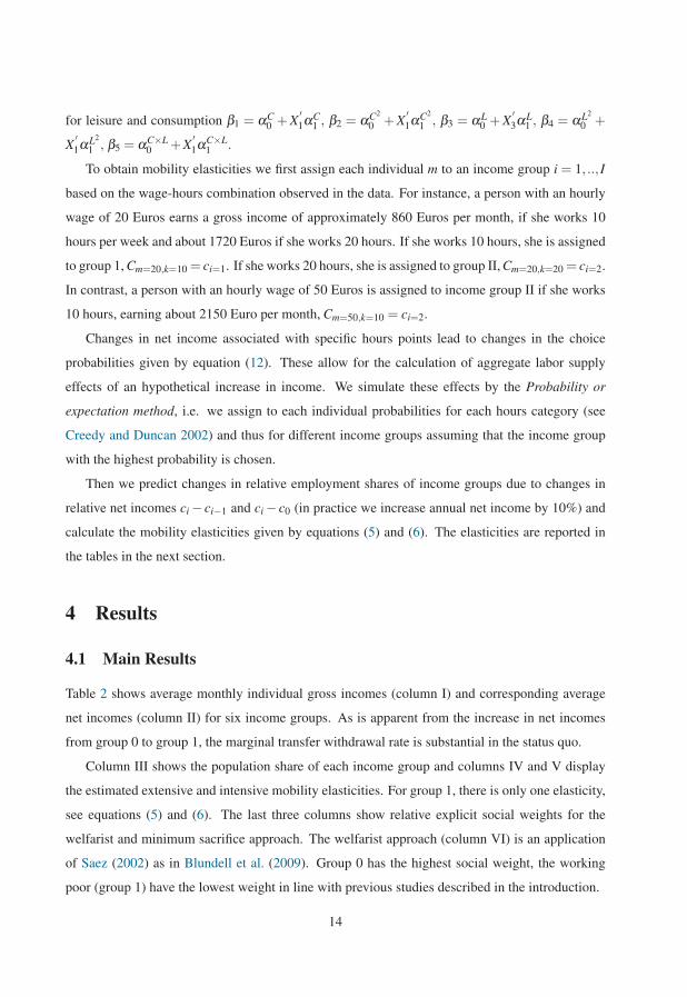
To obtain mobility elasticities we first assign each individual m to an income group i = 1, .., I

based on the wage-hours combination observed in the data. For instance, a person with an hourly

wage of 20 Euros earns a gross income of approximately 860 Euros per month, if she works 10

hours per week and about 1720 Euros if she works 20 hours. If she works 10 hours, she is assigned

to group 1, Cm=20,k=10 = ci=1. If she works 20 hours, she is assigned to group II, Cm=20,k=20 = ci=2.

In contrast, a person with an hourly wage of 50 Euros is assigned to income group II if she works

10 hours, earning about 2150 Euro per month, Cm=50,k=10 = ci=2.

Changes in net income associated with specific hours points lead to changes in the choice

probabilities given by equation (12). These allow for the calculation of aggregate labor supply

effects of an hypothetical increase in income. We simulate these effects by the Probability or

expectation method, i.e. we assign to each individual probabilities for each hours category (see

Creedy and Duncan 2002) and thus for different income groups assuming that the income group

with the highest probability is chosen.

Then we predict changes in relative employment shares of income groups due to changes in

relative net incomes ci − ci−1 and ci − c0 (in practice we increase annual net income by 10%) and

calculate the mobility elasticities given by equations (5) and (6). The elasticities are reported in

the tables in the next section.

4 Results

4.1 Main Results

Table 2 shows average monthly individual gross incomes (column I) and corresponding average

net incomes (column II) for six income groups. As is apparent from the increase in net incomes

from group 0 to group 1, the marginal transfer withdrawal rate is substantial in the status quo.

Column III shows the population share of each income group and columns IV and V display

the estimated extensive and intensive mobility elasticities. For group 1, there is only one elasticity,

see equations (5) and (6). The last three columns show relative explicit social weights for the

welfarist and minimum sacrifice approach. The welfarist approach (column VI) is an application

of Saez (2002) as in Blundell et al. (2009). Group 0 has the highest social weight, the working

poor (group 1) have the lowest weight in line with previous studies described in the introduction.

14

Table 2: Resulting Relative Weights for Different Justness Concepts

I II III IV V VI VII VIII

Group Gross Net Share η ζ Welfarist Minimum Sacrifice

Income Income Abs. Rel.

0 0 625 0.11 — — 1 1 1

1 1,137 949 0.19 0.08∗ 0.08∗ 0.29068 0.00077 0.29068

2 2,082 1,452 0.17 0.10 0.08 0.37729 0.00030 0.22023

3 2,697 1,755 0.19 0.09 0.07 0.37342 0.00020 0.19871

4 3,472 2,170 0.17 0.07 0.06 0.40902 0.00016 0.23123

5 5,458 3,257 0.18 0.05 0.08 0.38680 0.00009 0.27823

Note: German single households; own calculations based on the SOEP and the

STSM.∗Overall elasticity of group one is 0.16.

At the optimum, the welfarist weights show the costs of redistributing one Euro from individu-

als in group 0 to individuals in other groups. For instance, an increase in income for individuals in

group 1 would reduce income in group 0 by only 0.29 Euro because individuals would move from

group 0 to group 1, reducing the transfer burden of the state. Equivalently, the social planner val-

ues increasing the income for group 1 by one Euro 0.29 times as much as increasing the income

of group 0 by one Euro. The low weights for the working poor are related to the high marginal tax

rate for individuals moving from group 0 to group 1.17 Relative weights of the upper four income

groups are close to each other, in line with previous findings for Germany by Bargain et al. (2014).

Table C.1 in Appendix C shows the optimal welfarist tax schedule with weights decreasing

with income. The resulting optimal tax schedule implies a substantially lower marginal transfer

withdrawal rate for the working poor than in the status quo and higher net incomes for groups 1,

2, and 3. This underlines our finding that decreasing welfarist weights would imply lower transfer

withdrawal rates.

Column VII of Table 2 displays optimal weights for the minimum absolute sacrifice approach.

These weights show how much it costs in terms of the loss function of group 0 to reduce the loss

function for members of a particular group as defined in equation (10). We focus the interpretation

on the working groups as the unemployed are net recipients of transfers and thus ‘pay a positive

sacrifice’, see Section 2.2. A comparison of the weights of tax-paying groups shows the highest

17Ceteris paribus, higher elasticities and higher marginal tax rates imply a position further to the right of the Laffer

curve and thus lower social weights.

15

weight for the working poor, 0.00077, and decreasing weights with income. The social planner is

indifferent between imposing a slightly higher increase in the loss function on the working poor

and imposing four times this increase on the middle class (group 3). As the loss function increases

quadratically with taxes paid, the first derivative of the loss function with respect to consumption

for the working poor is relatively small. Consider the benchmark case with fixed incomes and the

same derivative of the loss function for all groups. In this case, all weights would be the same. In

our analysis the derivative of the loss function is lower for the working poor. Therefore, weights are

higher for this group.18 A similar reasoning applies to the other groups, which results in declining

social weights. Consequently, the minimum absolute sacrifice principle is in line with the 2015

German tax and transfer system.

Column VIII shows results for the minimum relative sacrifice principle. Note that the relative

weight of the group 1 is the same as for the welfarist approach. The reason is that we calibrated

f0 to equal f1, because y0 = 0. For the welfarist case with quasi-linear utility f1 always equals f0.

Therefore, the costs of increasing F1 by one relative to the costs of increasing F0 by one are the

same for the two concepts of justness. This is directly reflected by the relative weights, whereas

the absolute weights (not reported) differ. This calibration does not change the relations of weights

for groups 1-5.

Again, the working poor have the highest weight of the groups with a positive tax burden.

However, in contrast to the absolute sacrifice principle, weights are not decreasing with income

but U-shaped. Top income earners have relatively high weights according to the relative sacrifice

principle, because the tax paid is divided through a high consumption level. Thus a small increase

in taxes would not increase the loss function of this group by much. In fact, the middle class

(group 3) has the lowest weight according to this principle as one would have to redistribute less

to members of this group than to members of other groups in order to reduce their loss function by

a given amount. Thus, the 2015 German tax and transfer system does not imply decreasing social

weights under the minimum relative sacrifice principle.

In sum, we find that the minimum absolute sacrifice principle is in accordance with declining

social weights in the status quo. Thus, the minimization of absolute sacrifice is a good description

of the aims of the German society regarding the tax and transfer system.

18As the welfarist weights indicate, the deadweight loss of increasing taxes for group 1 is very high. If it was lower,

this group’s minimum sacrifice weight would be even higher.

16

4.2 Results for Subsamples

To explore whether the 2015 tax transfer schedule was designed according to a particular concept

of justness with focus on a specific group in mind, we split the sample into different groups. These

groups differ substantially regarding the income distribution and elasticities, which might lead to

different social weights.

First, the sample is split into females and males. We find that women have a more elastic labor

supply than men and lower incomes. Then, we present our results for East Germans and West

Germans, respectively. These two groups lived under different political systems for more than

40 years. We show that West Germans have higher incomes and less unemployment than East

Germans.

4.2.1 Results for Men and Women

In Table 3 we report results for the subsample of women without children, which we compare, in

the following, with the results for the main sample and, later, to men.

Table 3: Resulting Relative Weights for Different Justness Concepts for Women

without Children




0 0 615 0.05 — — 1 1 1

1 976 872 0.19 0.09∗ 0.09∗ 0.13061 0.00063 0.13061

2 1,903 1,331 0.20 0.12 0.10 0.16613 0.00015 0.05509

3 2,548 1,705 0.19 0.10 0.10 0.20113 0.00012 0.07105

4 3,342 2,079 0.23 0.07 0.10 0.18486 0.00007 0.06025

5 4,948 3,011 0.15 0.06 0.12 0.18374 0.00005 0.08011



As expected, gross and net incomes in all income groups are lower and labor supply elasticities

are slightly higher. For the welfarist case, the working groups have smaller weights relative to the

unemployed than in the main sample. As before, we find that the working poor have the lowest

weight. The finding that social weights for the minimum absolute sacrifice concept are decreasing

with income is robust for this subsample. As before, in the relative sacrifice case, the working poor

17

have the highest weights among working groups and top income earners have the second highest

weights.

Table 4: Resulting Relative Weights for Different Justness Concepts for Men

without Children




0 0 627 0.15 — — 1 1 1

1 1,265 1,038 0.17 0.05∗ 0.05∗ 0.49473 0.00109 0.49473

2 2,228 1,520 0.18 0.08 0.04 0.52023 0.00037 0.29738

3 2,875 1,837 0.16 0.07 0.04 0.52845 0.00025 0.28185

4 3,622 2,279 0.17 0.06 0.04 0.56493 0.00021 0.35296

5 6,124 3,581 0.16 0.05 0.06 0.52826 0.00010 0.39995



Table 4 shows results for the subsample of men. Incomes are higher and elasticities are lower

than for women. In the welfarist case, weights of working groups are higher than for women. This

is caused by lower elasticities, which lead to men being further on the left of the Laffer curve.

Nevertheless, the working poor again have the lowest weight. The finding that weights in the

absolute sacrifice case decrease with income holds for men as well. As in the welfarist case, the

weight of the working poor is higher for men than for women because male elasticities are lower.

Again, in the relative minimum sacrifice case, the working poor have the highest weight and the

middle class has the lowest weight of working groups.

4.2.2 Results for East and West Germany

Gross and net incomes are higher across all groups in West Germany (see Table 6) compared to

East Germany (see Table 5). In contrast to the main sample and the previously analyzed subsam-

ples, in the sample of East Germans the working poor are net transfer recipients and the marginal

withdrawal rate when moving from group 1 to group 2 is still substantial.

The welfarist weights show highest social weights for the unemployed and lowest for the work-

ing poor (group 1 in the West, groups 1 and 2 in the East). An increase in income for individuals

in group 1 by one Euro would reduce income in group 0 by only 0.27 Euro in West Germany and

18

by about 0.30 in East Germany. The relative weights of the four (three for East Germany) higher

income groups are very similar and higher than the weights for the working poor.

Table 5: Resulting Relative Weights for Different Justness Concepts for East

Germany




0 0 596 0.18 — — 1 1 1

1 774 851 0.17 0.10∗ 0.10∗ 0.30249 0.30249 0.30249

2 1,581 1,222 0.18 0.16 0.08 0.33926 0.00044 0.54047

3 2,200 1,594 0.17 0.13 0.08 0.40821 0.00032 0.63570

4 2,808 1,920 0.14 0.11 0.07 0.42652 0.00022 0.59342

5 4,039 2,625 0.16 0.09 0.08 0.40168 0.00013 0.58436



Table 6: Resulting Relative Weights for Different Justness Concepts for West

Germany




0 0 653 0.08 — — 1 1 1

1 1,408 1,072 0.21 0.07∗ 0.07∗ 0.26746 0.00040 0.26746

2 2,324 1,549 0.16 0.09 0.08 0.31984 0.00021 0.25346

3 2,907 1,857 0.19 0.08 0.08 0.31618 0.00015 0.25474

4 3,699 2,321 0.19 0.06 0.06 0.35053 0.00013 0.33020

5 6,010 3,519 0.17 0.05 0.08 0.32097 0.00006 0.35878



As in our main findings, optimal weights under minimum absolute sacrifice are decreasing in

both samples, though the weight of group 1 is closer to the weight of group 0 than is the case

for West Germany as group 1 in the East are net transfer recipients and thus enjoy a ‘positive tax

sacrifice’. Note that as group 1 in East Germany consists of transfer net recipients, f0 = f1 (see

equation (10)) for this group and thus the relative weight of group 1 is the same as in the welfarist

and relative sacrifice cases. Regarding groups with a positive tax burden, the weights imply that

19

the social planner is roughly indifferent between imposing a slight increase in the loss function

on the working poor (group 1) in West Germany and imposing five times this increase in the loss

function on group 2. For East Germany, the social planner is indifferent between imposing a slight

increase in the loss function for individuals in group 2 and an about 38 percent higher increase

in the loss function for individuals in group 3. This shows that the minimum absolute sacrifice

principle is in line with the 2015 German tax and transfer system for East and West Germans.

Results for the minimum relative sacrifice principle show that group 3 has the highest weight of

the groups with a positive tax burden in East Germany, while in West Germany weights for the top

income group are highest. The difference arises because top income earners in West Germany earn

considerably more than their East German counterparts. As explained in Section 4.1, this implies

higher weights for this justness concept because the denominator of the loss function is higher.

Thus, the German tax and transfer system does not result in decreasing social weights under the

minimum relative sacrifice principle.

4.3 Robustness and Extensions

4.3.1 Subjective Justness

Our framework allows using information on the level of taxes that is considered just by individuals

in the optimal tax formulae. We specify the justness functions similarly to the case of minimum

sacrifice and set as reference point the level of just after-tax income taken from the survey. Thus

the absolute formulation of the justness function is

Fi =−(cjusti − ci∗)

γ if cjusti ≥ ci∗ ,

Fi = (ci∗ − cjusti )δ if ci∗ > cjust

i , (14)

γ > 1,δ ≤ 1

and the relative one is

Fi =−(

cjusti − ci∗

ci∗

)γ

if cjusti ≥ ci∗ ,

Fi =

(ci∗ − cjust

ici∗

)δ

if ci∗ > cjusti > 0, (15)

γ > 1,δ ≤ 1.

20

The parameters are calibrated as for minimum sacrifice.

In the 2015 wave, the SOEP introduced new questions that ask what amount of income respon-

dents would consider just in their current occupation. In particular, individuals state how high their

gross income and net income would have to be in order to be just. A screenshot of this part of the

questionnaire is provided in Appendix B.19 Only the currently employed are asked questions about

what income they would consider as just.20

Compared to other approaches to obtain information about individuals’ ideas of justness, the

advantage of the question is that individuals do not need to have a worked out theory of just taxation

in mind to answer the question. Moreover, interviewees do not need a thorough understanding of

tax schedules.

Figure 1 shows the status quo of the German tax and transfer system and the just tax and transfer

system based on our sample. The first segment of the actual budget line is almost horizontal at a

net income of about 600 Euro due to the high transfer withdrawal rate. The slope of the budget

line is steeper further to the right, representing individuals who do not receive transfers, but pay

income taxes and social security contributions.

Gray circles represent the actual net incomes for given gross incomes. Some circles are crossed

by x. This means either that an individual considers his or her actual income just or the actual

income of another person. The 45 degree line marks the points where no taxes are paid. Points

above this line represent actual transfer recipients or those who deem receiving transfers as just.

However, most individuals perceive net incomes to be just, where taxes have to be paid. It is likely

that status quo bias explains this pattern. Nonetheless, the answers of the respondents reflect actual

perceptions of just incomes. The solid blue and the dashed red lines summarize this information.

The solid blue line depicts the average actual budget constraint for six income groups that we use

in the main analysis. The dashed red line shows the just budget constraint for the same groups. The

budget lines are based on averages for the groups. The just budget line is defined only for those with

19Since 2005 the SOEP includes a question on just income “Is the income that you earn at your current job just,

from your point of view?”. If respondents answer “No”, they are asked “How high would your net income have to be

in order to be just?” and since 2009 additionally “How high would your gross income have to be in order to be just?”.

The introduced justness question in 2005 was inspired by a perceived justness of earnings formula developed by Jasso

(1978). In 2015 these questions are revised to allow for more research topics and now all respondents are asked about

just gross and net income (see Appendix B).

20For the working poor, we add actual transfers to stated just net incomes, as these do not include transfers. Transfers

include Unemployment Benefit II, housing benefits.

21

0

1000

2000

3000

4000

5000

6000

Mon

thly

Net

Inco

me

0 1000 2000 3000 4000 5000 6000Monthly Gross Income

45 Degree LineActual IncomeJust IncomeActual Budget Line Group 0−5Just Budget Line Group 1−5

Figure 1: Just Net and Gross Incomes. Source: Own calculations based on SOEP

positive labor income and lies slightly above the actual budget line. This reflects the preferences

for paying less taxes. The distribution of net incomes for a given value of gross income is skewed

toward the no tax line. Deviations in this direction can be explained with allowances. The positive

skew of just net incomes is due to more people perceiving substantially higher net incomes as just

than substantially lower net incomes. The incidence of crossed circles, i.e., persons who perceive

their current income as just is higher below and around the average budget lines.

As only employed persons respond to the SOEP question about just net income, just net income

is set marginally above the actual average transfer income of group 0.21

21We experimented with different values for this number. While changing the just net income of group 0 has a

substantial impact on this group’s subjective social justness weights relative to other groups, the weights of other

groups relative to one another remain virtually the same.

22

Table 7: Resulting Relative Weights for Subjective Justness

I II III IV V VI VII

Group Net Just Net Difference η ζ Subjective Justness


0 779 784∗ 5 1 1

1 1,024 1,036 12 0.08 0.08 0.15341 0.26369

2 1,420 1,461 41 0.10 0.07 0.05241 0.17035

3 1,741 1,778 37 0.09 0.07 0.06424 0.31620

4 2,195 2,243 48 0.07 0.07 0.05207 0.40717

5 3,317 3,415 98 0.05 0.08 0.02475 0.43868

Note: German single households; own calculations based on the SOEP and

the STSM.∗Just net income for this group is set as explained in the text.

Table 7 shows social weights according to the absolute and relative subjective justness princi-

ples respectively. The sample—and thus means for current gross and net incomes—differs from

the main one as only individuals who report that their current gross income is just are used. The

subjective justness principle implies penalties for the deviation of net incomes from perceived just

net incomes. As discussed above, there is no information on perceived just net incomes of the

unemployed, so we focus on the interpretation of the social weights of working groups. For the

absolute justness principle, the working poor have the highest social weights of the working pop-

ulation because their average net income deviates from just net income by only 12 Euros. Social

weights are decreasing except for group 3, where the just net income is closer to actual net income

than is the case for groups 2 and 4. When considering relative deviations from just net income,

group 5 has the highest social weights of all working groups since the deviation from just income

is small relative to the high consumption level of this group.

4.3.2 Different Reference Points of Justness Functions

For the subjective justness approach, reference points of loss functions were taken directly from

survey data. It is interesting to see how the resulting weights for reference points taken from the

data compare with weights resulting from three classical scenarios of redistribution, where refer-

ence points of all income groups are higher than net income: First, the social planner assumes that

low income groups ask for less redistribution relative to the status quo than the high income groups.

Second, the low income groups ask for more redistribution than the high income groups. Third,

23

each income group wants to keep up with the next higher income group and asks for redistribution

to achieve the net incomes of the next higher group.

The absolute and relative loss functions are then given by

Fi =−(crefi − ci∗)

γ if crefi ≥ ci∗ ,

Fi = (ci∗ − crefi )δ if ci∗ > cref

i , (16)

γ > 1,δ ≤ 1

and

Fi =−(

crefi − ci∗

ci∗

)γ

if crefi ≥ ci∗ ,

Fi =

(ci∗ − cref

ici∗

)δ

if ci∗ > crefi > 0, (17)

γ > 1,δ ≤ 1,

where crefi is a calibrated reference point. Tables 8-10 show results for this exercise for the three

different cases.

Table 8: Case 1: Difference to Reference Points Increasing

with Income

I II III IV V

Group Net Reference Difference Abs. Rel.

Income Point

0 625 675 50 1 1

1 949 1,049 100 0.14534 0.32739

2 1,452 1,602 150 0.12576 0.66444

3 1,755 1,955 200 0.09335 0.71364

4 2,170 2,420 250 0.08180 0.9550

5 3,257 3,557 300 0.06447 1.73131

Note: German single households; own calculations based on

the SOEP and the STSM.

In Table 8 the reference point is set 50 Euros above the actual net income for group 0 and

the difference between actual income and the reference point increases by 50 Euros for every

income group until it reaches 300 Euros for group 5. For the absolute loss function, this results in

continuously decreasing social weights. In contrast, using the relative loss function, social weights

24

are increasing starting from group 1 as the increase in the denominator of the loss function more

than offsets the increase in the nominator with increasing net income. Nonetheless, the social

weight of group 0 is highest because reducing transfers for this group would be associated with a

substantial efficiency gain. Not reducing the transfer for this group is only reconcilable with a high

social weight. The exercise reported in Table 8 is related to the minimum sacrifice principle; if the

designer of the tax and transfer system followed the principle of minimum sacrifice, implicitly an

income-increasing difference between net income and reference point was chosen. Therefore, the

pattern for the minimum absolute sacrifice case in Table 2 is similar to this stylized case.

Table 9: Case 2: Difference to Reference Points Decreasing

with Income

I II III IV V


Income Point

0 625 1,625 1,000 1 1

1 949 1,119 170 1.70986 8.69247

2 1,452 1,612 160 2.35808 29.8062

3 1,755 1,905 150 2.48944 47.0166

4 2,170 2,310 140 2.92157 86.0196

5 3,257 3,387 130 2.97542 202.023



Table 10: Case 3: Reference Point Next Higher Income Group

I II III IV V


Income Point

0 625 949 324 1 1

1 949 1,452 503 0.18724 0.42840

2 1,452 1,755 303 0.40344 2.73546

3 1,755 2,170 415 0.29153 2.82285

4 2,170 3,257 1,087 0.12192 1.48678

5 3,257 4,757 1,500 0.08355 2.35881



Table 9 is the counterpart of Table 8 and shows resulting weights, where the difference between

actual net income and the reference points decreases with income. For group 0 this difference is

25

set to 1000 Euro in order to obtain continuously increasing social weights. Again, the efficiency

gain of reducing transfers for this group is very large and only when the reference point is far away

from actual income would the increase in the loss function offset this efficiency gain. This results

in a low relative social weight for this group. The relative loss function weights are increasing with

income too—to a much stronger degree than in case 1.

Finally, in Table 10, the net income of the next higher income group is taken as a reference

point, except for the highest income earners, where we set the reference point 1500 Euro above the

current net income. In this “Keeping up with the Joneses” scenario groups 2 and 3 have relatively

high weights for both absolute and relative loss functions as their net income is close to that of the

respective next higher income group.

4.3.3 Robustness

As for any loss function, results may differ depending on the properties of the function that is to

be minimized. We analyze the robustness of the obtained social weights for absolute minimum

sacrifice to different values of γ and δ (Tables 11 and 12). The result that social weights decline

with income is robust to a wide range of calibrations. This shows that the main result is not driven

by the parameter choice. Second, we set the intensive and extensive elasticities of all groups to

0.1 and show the results for all concepts of justness (Table D.1 in the appendix). The results are

very close to the main results. This shows that slight variations in the elasticities do not change the

results substantially.

Table 11: Resulting Relative Weights for Absolute

Minimum Sacrifice for Different Values of γ (δ = 1)

I II III IV

Group γ = 1.5 γ = 2 γ = 3 γ = 5

0 1 1 1 1

1 0.01413 0.00077 2.74×10−6 4.65×10−11

2 0.01002 0.00030 3.17×10−7 4.79×10−13

3 0.00811 0.00020 1.40×10−7 9.48×10−14

4 0.00756 0.00016 8.04×10−8 2.85×10−14

5 0.00550 0.00009 2.66×10−8 3.30×10−15

Note: German single households; own calculations based

on the SOEP and the STSM.

26

Table 12: Resulting Relative Weights for Absolute

Minimum Sacrifice for Different Values of δ (γ = 2)

I II III IV

Group δ = 0.1 δ = 0.3 δ = 0.5 δ = 1

0 1 1 1 1

1 2.35×10−7 2.56×10−6 1.55×10−5 0.00077

2 9.12×10−8 9.92×10−7 5.99×10−6 0.00030

3 6.04×10−8 6.56×10−7 3.96×10−6 0.00020

4 4.78×10−8 5.20×10−7 3.14×10−6 0.00016

5 2.68×10−8 2.91×10−7 1.76×10−6 0.00009



5 Conclusion

In this paper, we reconcile a puzzling contrast between current tax transfer practice in many coun-

tries and the common approach in the optimal taxation literature. While the literature commonly

assumes that the social planner values an additional unit of income for poor households more

than an additional unit of income for higher income households, commonly observed high transfer

withdrawal rates are only optimal if social weights of the working poor are very small. There-

fore, we compare alternative approaches to welfarism and calculate the implied social weights.

We formulate the problem of a social planner for two distinct concepts of justness: the welfarist

approach, where the social planner maximizes the weighted sum of utility; alternatively, the mini-

mum sacrifice concept where the social planner minimizes the weighted sum of absolute or relative

(tax-)sacrifice. Moreover, we illustrate how subjective justness can be used in our model where

the social planner minimizes absolute or relative deviations from perceived just net income. Of

course, all approaches maintain budget neutrality and account for labor supply reactions.

Like the existing literature, we find that the 2015 German tax and transfer system implies very

low social weights for the working poor according to the welfarist criterion. The social planner

values increasing the income for the working poor by one Euro 0.75 times as much as increasing

the income of top earners by one Euro. This implies that an additional Euro of consumption for

the working poor is valued less than marginal consumption of top income earners.

In contrast, the current tax-transfer practice can be reconciled as optimal and in line with de-

creasing social weights under the minimum absolute sacrifice criterion, under which the social

planner minimizes a function that puts an increasing penalty on deviations from zero sacrifice. In

27

this case, the social planner is indifferent between a slight increase in the loss function for the

working poor and imposing four times this additional increase in the loss function on the middle

class.

References

AABERGE, R., AND U. COLOMBINO (2014): “Labour supply models,” in Handbook of microsim-

ulation modelling, ed. by C. O’Donoghue, vol. 293 of Contributions to economic analysis, 167–

221. Emerald Group Publishing. Cited on pages 3 and 11.

AABERGE, R., U. COLOMBINO, AND S. STRØM (2000): “Labor supply responses and welfare

effects from replacing current tax rules by a flat tax: empirical evidence from Italy, Norway and

Sweden,” J. Population Econ., 13(4), 595–621. Cited on page 3.

AABERGE, R., J. K. DAGSVIK, AND S. STRØM (1995): “Labor supply responses and welfare

effects of tax reforms,” Scand. J. Econ., 97(4), 635–659. Cited on page 11.

BARGAIN, O., M. DOLLS, D. NEUMANN, A. PEICHL, AND S. SIEGLOCH (2014): “Comparing

Inequality Aversion across Countries when Labor Supply Responses Differ,” International Tax

and Public Finance, 21(5), 845–873. Cited on pages 4, 5, and 13.

BERLIANT, M., AND M. GOUVEIA (1993): “Equal sacrifice and incentive compatible income

taxation,” Journal of Public Economics, 51, 219–240. Cited on page 3.

BLUNDELL, R., M. BREWER, P. HAAN, AND A. SHEPHARD (2009): “Optimal Income Taxation

of Lone Mothers: An Empirical Comparison of the UK and Germany,” Economic Journal,

119(535), F101–F121. Cited on pages 2, 4, 6, 9, 11, and 12.

BOURGUIGNON, F., AND A. SPADARO (2012): “Tax–Benefit Revealed Social Preferences,” Jour-

nal of Economic Inequality, 10(1), 75–108. Cited on page 4.

BRITZKE, J., AND J. SCHUPP (eds.) (2017): SOEP Wave Report 2016. Cited on page 10.

CHRISTENSEN, L. R., D. W. JORGENSON, AND L. J. LAU (1975): “Transcendental Logarithmic

Utility Functions,” The American Economic Review, 65(3), 367–383. Cited on page 11.

COLOMBINO, U., AND D. DEL BOCA (1990): “The effect of taxes on labor supply in Italy,” J.

Human Res., 25(3), 390–414. Cited on page 3.

28

CREEDY, J., AND A. DUNCAN (2002): “Behavioural microsimulation with labour supply re-

sponses,” J. Econ. Surveys, 16(1), 1–39. Cited on page 12.

DA COSTA, C., AND T. PEREIRA (2014): “On the efficiency of equal sacrifice income tax sched-

ules,” European Economic Review, 70, 399–418. Cited on page 3.

DIAMOND, P. (1980): “Income Taxation with Fixed Hours of Work,” Journal of Public Eco-

nomics, 13(1), 101 – 110. Cited on page 5.

HAAN, P., AND K. WROHLICH (2010): “Optimal Taxation: The Design of Child-Related Cash

and In-Kind Benefits,” German Economic Review, 11, 278–301. Cited on page 11.

HECKMAN, J. J. (1979): “Sample selection bias as a specification error,” Econometrica, 47(1),

153–161. Cited on page 11.

IMMERVOLL, H., H. J. KLEVEN, C. T. KREINER, AND E. SAEZ (2007): “Welfare Reform in

European Countries: A Microsimulation Analysis,” Economic Journal, 117(516), 1–44. Cited

on page 4.

JASSO, G. (1978): “On the Justice of Earnings: A New Specification of the Justice Evaluation

Function,” American Journal of Sociology, 83, 1398–1419. Cited on page 19.

JESSEN, R., D. ROSTAM-AFSCHAR, AND V. STEINER (2017): “Getting the Poor to Work: Three

Welfare Increasing Reforms for a Busy Germany,” Public Finance Analysis, 73(1), 1–41. Cited

on page 11.

KAHNEMAN, D., AND A. TVERSKY (1979): “Prospect Theory: An Analysis of Decision under

Risk,” Econometrica, 47(2), 263–291. Cited on page 9.

LIEBIG, S., AND C. SAUER (2016): Sociology of Justice 37–59. Springer New York, New York,

NY. Cited on page 3.

LOCKWOOD, B. B. (2016): “Optimal Income Taxation with Present Bias,” Working paper. Cited

on page 2.

LOCKWOOD, B. B., AND M. WEINZIERL (2016): “Positive and Normative Judgments Implicit

in U.S. Tax Policy, and the Costs of Unequal Growth and Recessions,” Journal of Monetary

Economics, 77, 30–47. Cited on page 4.

29

MCFADDEN, D. (1974): “Conditional logit analysis of qualitative choice behavior,” in Frontiers

in econometrics, ed. by P. Zarembka, 105–142. Academic Press, New York. Cited on page 11.

MILL, J. S. (1871): Principle of Political Economy. Longmans Green & Co., London. Cited on

page 3.

MIRRLEES, J. A. (1971): “An Exploration in the Theory of Optimum Income Taxation,” Review

of Economic Studies, 38(2), 175–208. Cited on page 5.

MUSGRAVE, R. A., AND P. B. MUSGRAVE (1973): Public Finance in Theory and Practice.

McGraw-Hill, New York. Cited on page 3.

RICHTER, W. F. (1983): “From Ability to Pay to Concepts of Equal Sacrifice,” Journal of Public

Economics, 20, 211–229. Cited on page 3.

SAEZ, E. (2001): “Using Elasticities to Derive Optimal Income Tax Rates,” Review of Economic

Studies, 68, 205–229. Cited on page 2.

(2002): “Optimal Income Transfer Programs: Intensive Versus Extensive Labor Supply

Responses,” The Quarterly Journal of Economics, 117(3), 1039–1073. Cited on pages 1, 2, 4,

5, 6, 7, 8, 12, and 31.

SAEZ, E., AND S. STANTCHEVA (2016): “Generalized Social Marginal Welfare Weights for Op-

timal Tax Theory,” American Economic Review, 106(1), 24–45. Cited on pages 2 and 3.

STEINER, V., K. WROHLICH, P. HAAN, AND J. GEYER (2012): “Documentation of the Tax-

Benefit Microsimulation Model STSM: Version 2012,” Data Documentation 63, DIW Berlin,

German Institute for Economic Research. Cited on page 11.

VAN SOEST, A. (1995): “Structural Models of Family Labor Supply: A Discrete Choice Ap-

proach,” Journal of Human Resources, 30(1), 63–88. Cited on page 11.

WAGNER, G. G., J. R. FRICK, AND J. SCHUPP (2007): “The German Socio-Economic Panel

Study (SOEP): Scope, Evolution and Enhancements,” Journal of Applied Social Science Studies,

127(1), 139–169. Cited on page 10.

WEINZIERL, M. (2014): “The Promise of Positive Optimal Taxation: Normative Diversity and a

Role for Equal Sacrifice,” Journal of Public Economics, 118(C), 128–142. Cited on pages 3

and 9.

30

YOUNG, P. (1988): “Distributive Justice in Taxation,” Journal of Economic Theory, 44, 321–335.

Cited on page 3.

Appendix

A Optimal Tax Formulae in the General Model

Behavioral reactions imply that hi changes in case of a change in Ti. Using the product rule and

assuming that marginal movers do not impact the objective function, the first order condition with

respect to Ti is obtained as

∫M

μm fmdν(m) = λ

(hi −

I

∑j=0

Tj∂h j

∂ci

), (18)

where λ is the multiplier of the budget constraint. The first order condition with respect to λ

is the budget constraint. Assuming fi = fm, reorganizing (18), and defining the average explicit

social weights as ei = μi/λhi yields

(1− ei fi)hi =I

∑j=0

Tj∂h j

∂ci. (19)

The assumption of no income effects implies that only hi−1, hi, hi+1, and h0 change when Ti

changes. If we assume that hi can be expressed as a function depending on the difference to the the

adjacent income groups and the unemployed hi(ci+1−ci,ci−ci−1,ci−c0), equation (19) simplifies

to

(1− ei fi)hi = T0∂h0

∂ (ci − c0)+Ti

∂hi

∂ (ci − c0)−Ti+1

∂hi+1

∂ (ci+1 − ci)−Ti

∂hi

∂ (ci+1 − ci)(20)

+ Ti∂hi

∂ (ci − ci−1)+Ti−1

∂hi−1

∂ (ci − ci−1).

Using the facts that ∂hi∂ (ci−c0)

= − ∂h0

∂ (ci−c0),

∂hi+1

∂ (ci+1−ci)= − ∂hi

∂ (ci+1−ci), ∂hi

∂ (ci−ci−1)= − ∂hi−1

∂ (ci−ci−1), we

can write after rearranging

(1− ei fi)hi = (Ti −T0)∂hi

∂ (ci − c0)− (Ti+1 −Ti)

∂hi+1

∂ (ci+1 − ci)+(Ti −Ti−1)

∂hi

∂ (ci − ci−1).(21)

Using the definition of the elasticities (5) and (6), we obtain for each group after reorganizing

31

Ti −Ti−1

ci − ci−1=

1

ζihi{(1− ei fi)hi −ηihi

Ti −T0

ci − c0+ζi+1hi+1

Ti+1 −Ti

ci+1 − ci

}. (22)

Note that, by setting e0 = ei = 0, we obtain the Laffer-condition

Ti −Ti−1

ci − ci−1=

1

ζi+

ζi+1hi+1

ζihi

Ti+1 −Ti

ci+1 − ci− ηi

ζi

Ti −T0

ci − c0. (23)

Substituting the equivalent of (22) for the next group i+1 in (22) and simplifying gives

Ti −Ti−1

ci − ci−1=

1

ζihi

{(1− ei fi)hi +(1− ei+1 fi+1)hi+1 (24)

−ηihiTi −T0

ci − c0−ηi+1hi+1

Ti+1 −T0

ci+1 − c0+ζi+2hi+2

Ti+2 −Ti+1

ci+2 − ci+1

}.

Recursive insertion and simplifying gives the I formulae (7) that must hold if function (1) is

optimized.

32

B Questionnaire

Figure B.1: The Question for Justness. Source: Official SOEP Questionnaire

C Optimal Welfarist Tax Schedule

Table C.1 shows the optimal welfarist tax schedule, where, following Saez (2002), implicit welfare

weights are set according to the formula

gi =1

λc0.25i

(25)

and the shares of income groups are determined endogenously by

hi = h0i

(ci − c0

c0i − c0

0

)ηi

, (26)

where the superscript 0 denotes values in the status quo. The simulation was done achieving

budget neutrality and setting net income of group 0 to the status quo, as a deviation from this is not

politically feasible.

33

Table C.1: Optimal Welfarist Tax Schedule

Group Gross Net Share Optimal Optimal Relative

Income Income Net Income Share Weight

0 0 625 0.11 625 0.09 1

1 1,137 949 0.19 1,260 0.20 0.84

2 2,082 1,452 0.17 1,629 0.17 0.79

3 2,697 1,755 0.19 1,837 0.19 0.76

4 3,472 2,170 0.17 2,047 0.17 0.74

5 5,458 3,257 0.18 2,826 0.18 0.69

Note: German single households; own calculations based on the SOEP

and the STSM.

D Further Sensitivity Checks

Table D.1: Resulting Relative Weights for Different

Justness Concepts with Elasticities set to 0.1

I II III IV V

Group η ζ Welfarist Minimum Sacrifice

Abs. Rel.

0 — — 1 1 1

1 0.1∗ 0.1∗ 0.22027 0.00059 0.22027

2 0.1 0.1 0.33434 0.00027 0.19516

3 0.1 0.1 0.31926 0.00017 0.16989

4 0.1 0.1 0.33459 0.00013 0.18916

5 0.1 0.1 0.30932 0.00007 0.22250

Note: German single households; own calculations

based on the SOEP and the STSM.∗Overall elasticity of group one is 0.2.

34

Optimal Taxation Under Different Concepts of Justness · RWI is funded by the Federal Government...

Documents

Transcript of Optimal Taxation Under Different Concepts of Justness · RWI is funded by the Federal Government...