Optimal sensitivity based on IPOPT

Math. Prog. Comp. (2012) 4:307–331DOI 10.1007/s12532-012-0043-2

FULL LENGTH PAPER

Optimal sensitivity based on IPOPT

Hans Pirnay · Rodrigo López-Negrete ·Lorenz T. Biegler

Received: 14 April 2011 / Accepted: 22 May 2012 / Published online: 20 June 2012© Springer and Mathematical Optimization Society 2012

Abstract We introduce a flexible, open source implementation that provides theoptimal sensitivity of solutions of nonlinear programming (NLP) problems, and isadapted to a fast solver based on a barrier NLP method. The program, called sIPOPTevaluates the sensitivity of the Karush–Kuhn–Tucker (KKT) system with respect toperturbation parameters. It is paired with the open-source IPOPT NLP solver andreuses matrix factorizations from the solver, so that sensitivities to parameters aredetermined with minimal computational cost. Aside from estimating sensitivities forparametric NLPs, the program provides approximate NLP solutions for nonlinearmodel predictive control and state estimation. These are enabled by pre-factored KKTmatrices and a fix-relax strategy based on Schur complements. In addition, reducedHessians are obtained at minimal cost and these are particularly effective to approx-imate covariance matrices in parameter and state estimation problems. The sIPOPTprogram is demonstrated on four case studies to illustrate all of these features.

Keywords NLP · Sensitivity · Interior point

Mathematics Subject Classification (2000) 90C30 · 90C31 · 90C51 · 90-08

H. PirnayAVT-Process Systems Engineering, RWTH Aachen University,Turmstr. 46, Aachen 52064, Germany

R. López-Negrete · L. T. Biegler (B)Department of Chemical Engineering, Carnegie Mellon University,5000 Forbes Avenue, Pittsburgh, PA 15213, USAe-mail: [email protected]

123

308 H. Pirnay et al.

1 Introduction

Sensitivity analysis for nonlinear programming problems is a key step in any optimi-zation study. This analysis provides information on regularity and curvature condi-tions at Karush–Kuhn–Tucker (KKT) points, assesses which variables play dominantroles in the optimization, and evaluates first-order sensitivities (i.e., first derivatives ordirectional derivatives) of the solution vector with respect to perturbation parameters.Moreover, for NLP algorithms that use exact second derivatives, sensitivity can beimplemented very efficiently within NLP solvers and provide valuable informationwith very little added computation. In this study we discuss a capability for sensi-tivity analysis that is coupled to IPOPT [1], a barrier NLP solver that incorporates afilter-based line search.

The basic sensitivity strategy for NLP solvers is derived through application ofthe implicit function theorem (IFT) to the KKT conditions of a parametric NLP. Asshown in Fiacco [2], sensitivities can be obtained from a solution with suitable regular-ity conditions, merely by solving a linearization of the KKT conditions. Nevertheless,relaxation of some of these regularity conditions induces singularity and inconsis-tency in this linearized system, and may make the sensitivity calculation much moredifficult. Reviews of sensitivity analysis can be found in Fiacco [2], Fiacco and Ish-izuka [3], and Büskens and Maurer [4]. More advanced cases have been analyzed byKyparisis [5], Kojima [6], Kojima and Hirabayashi [7], and Jongen et al. [8,9]. Anearly implementation of sensitivity analysis applied to barrier methods can be foundin Fiacco and Ghaemi [10].

For over 25 years, NLP sensitivity analysis has been applied to numerous appli-cations in process engineering, as these can be viewed as parametric programs, withparameters that represent uncertain data or unknown inputs. These applications includeflowsheet optimization [11,12], steady state real-time optimization [13], robust optimi-zation and parameter estimation, nonlinear model predictive control [14], and dynamicreal-time optimization [15].

With improvements in fast Newton-based barrier methods, such as IPOPT, sen-sitivity information can be obtained very easily. As a result, fast on-line algorithmscan be constructed where more expensive optimization calculations can be solved inadvance, and fast updates to the optimum can be made on-line. This has motivatedalgorithms for control, estimation and dynamic optimization that execute large opti-mization models with very little on-line computation [16]. This has been especiallysuccessful for so-called advanced step strategies that work with large, sparse NLPsolvers. To obtain the sensitivity information, we exploit the full space informationavailable through the linearization of the KKT conditions that appears naturally in thesolution process. The resulting code that incorporates this strategy, called sIPOPT , isimplemented in C++ and appended to the NLP solver IPOPT.

This study is organized as follows. In Sect. 2, we derive the equations that pro-vide sensitivity information from perturbation of the KKT conditions. In addition, theimplementation of the numerical solution and the handling of changes in the activeset are discussed. This is based on a fix-relax strategy that modifies the KKT systemthrough a Schur complement strategy. A parametric programming case study is pre-sented at the end of this section to illustrate the strategy and the software. Section 3

123

Optimal sensitivity based on IPOPT 309

presents two case studies that showcase different facets of the implementation. Thefirst example deals with a nonlinear model predictive controller (NMPC) for a contin-uous stirred tank reactor (CSTR), where set-point changes occur. In the next example,the sensitivity based update is applied to NMPC control of a large-scale distillationcolumn model. Using the advanced step approach, the controller stays close to theideal case, where we assumed that there are no computational delays. Section 4 thendevelops a straightforward procedure to extract the inverse of the reduced Hessianfrom the pre-factored KKT system. As an illustration, the last case study deals with aparameter estimation problem for a small dynamic system. Here the sensitivity-basedextraction of the inverse reduced Hessian leads to an estimate of the covariance matrixfor the estimated parameters. The paper then concludes with a discussion of thesecontributions and future work.

2 Sensitivity concepts and derivation

The following are well known properties of nonlinear programs. They are shown herefor convenience as they will be used for the derivations in the following sections.

Consider the parametric nonlinear program of the form:

minx f (x; p) (1a)

s.t. c(x; p) = 0, x ≥ 0 (1b)

with the variable vector x ∈ Rnx , the vector of perturbation parameters p ∈ R

n p , andequality constraints c(x; p) : R

nx +n p → Rm . The IPOPT NLP algorithm substitutes

a barrier function for the inequality constraints and solves the following sequence ofproblems with μ� → 0:

minx f (x; p) − μ�

nx∑

i=1

ln(xi ) (2a)

s.t. c(x; p) = 0. (2b)

The sIPOPT program relies on the IPOPT solver [1], which solves (1) through asequence of barrier problems (2). Having x∗ = x(p0), the solution of (1) with p = p0(the nominal value), sIPOPT computes the sensitivity information of this solutionwith respect to p, given by the first derivatives dx(p0)

dp and

d f (x∗; p0)

dp= ∂ f (x∗; p0)

∂p+ dx(p0)

dp

∂ f (x∗; p0)

∂x. (3)

To obtain these derivatives, we first consider properties of the solutions of (1) obtainedby IPOPT when p = p0 [2,17]. We then derive the sensitivity calculation implementedin sIPOPT based on these properties in Sect. 2.2.

In Sect. 2.4, we consider finite perturbations of the parameters p, which can lead tochanges in active sets for x(p). To deal with this issue, we need to relax the conditions

123


of Sect. 2.2 to consider cases where the active set is nonunique and first derivativesno longer exist. In particular, we discuss relaxed conditions under which directionalderivatives, which reflect the sensitivity of the x∗ to directional perturbations of p,can still be obtained. Although automatic calculation of these directional derivativeshas not yet been implemented in sIPOPT , Sect. 2.5 describes an enabling tool, the“fix-relax” strategy, that allows more general sensitivity strategies to be implemented.Also, more details on the implementation and features of sIPOPT are described inSect. 2.7.

2.1 Sensitivity properties

For the NLP (1), the KKT conditions are defined as:

∇x L(x∗, λ∗, ν∗; p0) = ∇x f (x∗; p0) + ∇x c(x∗; p0)λ∗ − ν∗ = 0 (4a)

c(x∗; p0) = 0 (4b)

0 ≤ ν∗ ⊥ x∗ ≥ 0 (4c)

For the KKT conditions to serve as necessary conditions for a local minimumof (1), constraint qualifications are needed, such as the Linear Independence Con-straint Qualification (LICQ) or the Mangasarian–Fromowitz Constraint Qualification(MFCQ). Note that in the following definitions Q j means the j th column of a givenmatrix Q, and I represents the identity matrix of appropriate dimension.

Definition 1 (Linear independence constraint qualification (LICQ)) Given a localsolution of (1), x∗ with a set of active bound indices A (x∗) ⊆ {1, . . . , n} with x∗

j =0, j ∈ A (x∗) and nb = |A (x∗)|. These active bounds can be written as ET x∗ = 0,where Ei = I ji for i = 1, . . . , nb and ji is the i th element of A (x∗). The LICQ isthen defined by linear independence of the active constraint gradients, i.e.,

[∇x c(x∗; p0) | E]

has full column rank. Satisfaction of the LICQ leads to unique multipliers λ∗, ν∗ at aKKT point.

Definition 2 (Mangasarian–Fromowitz constraint qualification (MFCQ)) Given alocal solution of (1), x∗ and an active set, with ET x∗ = 0, the MFCQ is definedby linear independence of the equality constraint gradients and the existence of asearch direction d, such that:

ET d > 0,∇x c(x∗; p0)T d = 0.

In addition, we consider the following sufficient second-order conditions.

Definition 3 (Strong second-order sufficient conditions (SSOSC)) Given x∗ and somemultipliers λ∗, ν∗ that satisfy the KKT conditions (4), then the SSOSC hold if

123


dT ∇xx L(x∗, λ∗, ν∗; p0)d > 0 for all d = 0 with ∇x c(x∗)T d = 0,

di = 0 for ν∗i > 0. (5)

We define L M(x; p) as the set of multipliers (λ, ν) such that the KKT conditionshold at x for parameter p with (λ, ν) [5]. If the MFCQ and SSOSC hold at (x∗, p0)

then there exists a unique, continuous path of optimal points x(p) of (1) in a neigh-borhood of (x∗, p0) [18]. In addition, the point-to-set map (x, p) → L M(x; p) isthen upper semi-continuous in a neighborhood of (x∗, p0) and the set L M(x(p); p)

is a nonempty polyhedron [19]. Finally, we define Kex (x(p), p) as the set of vertexpoints of the polyhedron L M(x(p); p).

The conditions defined above allow us to state the following property on the solutionbarrier problems (2).

Property 1 (Properties of the central path/barrier trajectory) Consider problem (1)with f (x; p) and c(x; p) at least twice differentiable in x and once in p. Let x∗ be alocal constrained minimizer of (1) with the following sufficient optimality conditionsat x∗:

– x∗ is a KKT point that satisfies (4),– the LICQ holds at x∗,– strict complementarity (SC) holds at x∗ for the bound multipliers ν∗, i.e., x∗

i +ν∗i >

0, and– The SSOSC holds for x∗, λ∗, and ν∗ that satisfy (4).

If we now solve a sequence of barrier problems (2) with p = p0 and μ� → 0, then:

1. There is at least one subsequence of solutions to (2), x(μ�; p0), converging tox∗.

2. For every convergent subsequence, the corresponding sequence of barrier multi-plier approximations is bounded and converges to multipliers satisfying the KKTconditions for x∗.

3. A unique, continuously differentiable vector function x(μ, p0), the minimizer of(2), exists for μ > 0 in a neighborhood of μ = 0.

4. limμ→0+ x(μ; p0) = x∗.5. ‖x(μ, p0) − x∗‖ = O(μ).

Proof The proof follows by noting that the LICQ implies the MFCQ and by invokingTheorem 3.12 and Lemma 3.13 in [17]. �

This property indicates that nearby solutions of (2) provide useful information forbounding properties for (1) for small positive values of μ. For such cases we nowconsider the sensitivity of these solutions with respect to changes in values of p.

Property 2 (Sensitivity properties) For problem (1) assume that f (x; p) and c(x; p)

are k times differentiable in p and k +1 times differentiable in x. Also, let the assump-tions of Property 1 hold for problem (1) with p = p0, then at the solution:

– x∗ = x(p0) is an isolated minimizer and the associated multipliers λ∗ and ν∗ areunique.

123


– For some p in a neighborhood of p0 there exists a k times differentiable function

s(p)T = [x(p)T λ(p)T ν(p)T ]

that corresponds to a locally unique minimum for (1) and s(p0) = s∗.– For p near p0 the set of active inequalities is unchanged and complementary

slackness holds.

Proof The result follows directly from Theorem 3.2.2 and Corollary 3.2.5 in [2]. � We now consider the barrier formulation and relate sensitivity results between (1)

and (2) with the following result.

Property 3 (Barrier sensitivity properties) For the barrier problem (2) assume thatf (x; p) and c(x; p) are k times differentiable in p and k + 1 times differentiable inx. Also, let the assumptions of Property 1 hold for problem (1), then at the solution of(2) with a small positive μ:

– x(μ; p0) is an isolated minimizer and the associated barrier multipliers λ(μ; p0)

and ν(μ; p0) are unique.– For some p in a neighborhood of p0 there exists a k times differentiable function

s(μ; p)T =[x(μ; p)T λ(μ; p)T ν(μ; p)T

]

that corresponds to a locally unique minimum for (2).– s(0; p0) ≡ limμ→0,p→p0 s(μ; p) = s∗.

Proof The result follows from Theorem 6.2.1 and Corollary 6.2.2 in [2]. These resultswere proved first for a mixed penalty function, but the proofs are easily modified todeal with barrier functions. �

2.2 Barrier sensitivity calculation

Calculation of the sensitivity of the primal and dual variables with respect to p nowproceeds from the implicit function theorem (IFT) applied to the optimality conditionsof (2) at p0. Defining the quantities:

M(s(μ; p0)) =⎡

⎣W (s (μ; p0)) A (x (μ; p0)) −IA (x (μ; p0))

T 0 0V (μ; p0) 0 X (μ; p0)

⎤

⎦ (6)

and

Np(s(μ; p0)) =⎡

⎣∇xp L(s(μ; p0))

∇pc(x(μ; p0))T

0

⎤

⎦, Nμ =⎡

⎣00

−μe

⎤

⎦ (7)

123


where W (s(μ; p0)) denotes the Hessian ∇xx L(x, λ, ν) of the Lagrangian functionevaluated at s(μ; p0), A(x(μ; p0)) = ∇x c(x) evaluated at x(μ; p0), X = diag{x}and V = diag{ν}, application of IFT leads to:

M(s(μ; p0))ds(μ; p0)

dp

T

+ Np(s(μ; p0)) = 0. (8)

When the assumptions of Property 1 hold, M(s(μ; p0)) is nonsingular and thesensitivities can be calculated from:

ds(μ; p0)

dp

T

= −M (s (μ; p0))−1 Np (s (μ; p0)) . (9)

Depending of the choice of the sparse solver selected in IPOPT, one can oftencheck the assumptions of the LICQ, SC and SSOSC at the solution of (2) by usingan estimate of the inertia of M (see [1]). Moreover, in IPOPT M(s(μ; p0)) is directlyavailable in factored form from the solution of (2), so the sensitivity can be calculatedthrough a simple backsolve. For small values of μ and ‖p − p0‖ it can be shown fromthe above properties [2] that

s(μ; p) = s(μ; p0) − M(s(μ; p0))−1 Np(s(μ; p0))(p − p0) + o‖p − p0‖ (10)

or

s(0; p) = s(μ; p0) − M(s(μ; p0))−1 [

Np(s(μ; p0))(p − p0) + Nμ

]

+o‖p − p0‖ + o(μ). (11)

Finally, the implementation of NLP sensitivity is simplified if the parameters canbe separated in the NLP formulation. In this case, we write:

minx,w f (x, w) (12a)

s.t. c(x, w) = 0, x ≥ 0 (12b)

w − p0 = 0 (12c)

Note that the NLP solution is equivalent to (1), and it is easy to see that the NLPsensitivity is equivalent as well. Writing the KKT conditions for (12) gives:

∇x f (x, w) + ∇x cT (x, w)λ − ν = 0 (13a)

∇w f (x, w) + ∇wcT (x, w)λ + λ = 0 (13b)

c(x) = 0 (13c)

X V e = 0 (13d)

w − p0 = 0. (13e)

In (13a) λ represents the multiplier corresponding to the equation w − p0 = 0. Forthe Newton step we write:

123


⎡

⎢⎢⎢⎢⎣

W ∇xw L(x, w, λ, ν) A −I 0∇wx L(x, w, λ, ν) ∇ww L(x, w, λ, ν) ∇wc(x, w) 0 I

AT ∇wc(x, w)T 0 0 0V 0 0 X 00 I 0 0 0

⎤

⎥⎥⎥⎥⎦

⎡

⎢⎢⎢⎢⎣

�x�w

�λ

�ν

�λ

⎤

⎥⎥⎥⎥⎦=

⎡

⎢⎢⎢⎢⎣

0000

�p

⎤

⎥⎥⎥⎥⎦.

(14)

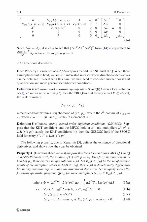
Since �w = �p, it is easy to see that [�xT �λT �νT ]T from (14) is equivalent tods(μ;p0)

dp

T�p obtained from (8) as μ → 0.

2.3 Directional derivatives

From Property 1, existence of ds∗/dp requires the SSOSC, SC and LICQ. When theseassumptions fail to hold, we are still interested in cases where directional derivativescan be obtained. To deal with this case, we first need to consider another constraintqualification and more general second-order conditions.

Definition 4 (Constant rank constraint qualification (CRCQ)) Given a local solutionof (1), x∗ and an active set, A (x∗), then the CRCQ holds if for any subset K ⊂ A (x∗),the rank of matrix

[∇x c(x; p) | EK ]

remains constant within a neighborhood of (x∗, p0), where the i th column of EK ,i =I ji where i = 1, . . . |K | and ji is the i th element of K .

Definition 5 (General strong second-order sufficient conditions (GSSOSC)) Sup-pose that the KKT conditions and the MFCQ hold at x∗, and multipliers λ∗, ν∗ ∈L M(x∗; p0) satisfy the KKT conditions (4), then the GSSOSC hold if the SSOSChold for every λ∗, ν∗ ∈ L M(x∗; p0).

The following property, due to Kyparisis [5], defines the existence of directionalderivatives, and shows how they can be obtained.

Property 4 (Directional derivatives) Suppose that the KKT conditions, MFCQ, CRCQand GSSOSC hold at x∗, the solution of (1) with p = p0. Then for p in some neighbor-hood of p0, there exists a unique solution x(p). Let Kex (x∗, p0) be the set of extremepoints of the multiplier values in L M(x∗; p0), then x(p) is directionally differentia-ble in any direction �p = 0 and the directional derivative �x uniquely solves thefollowing quadratic program (QPs), for some multipliers (λ, ν) ∈ Kex (x∗, p0).

min�x � = �x T ∇xp L(s(p0))�p + 1

2�x T ∇xx L(s(p0))�x (15a)

s.t. ∇pc(x∗; p0)T �p + ∇x c(x∗; p0)

T �x = 0 (15b)

�x j ≥ 0, j ∈ A (x∗) (15c)

�x j = 0, for some ν j ∈ Kex (x∗, p0), with ν j > 0. (15d)

123


This property provides the weakest assumptions under which a unique directionalderivative can be shown [5,6]. Note that the GSSOSC assumption provides sufficientconditions for positive definiteness of the Hessian in the null space of the stronglyactive bounds (for every x∗

i = 0, there exists ν∗i > 0). This property, along with the

MFCQ and the CRCQ, allows uniqueness of the directional derivative to be proved.Examples on the application of (15) to calculate directional derivatives are given in[5].

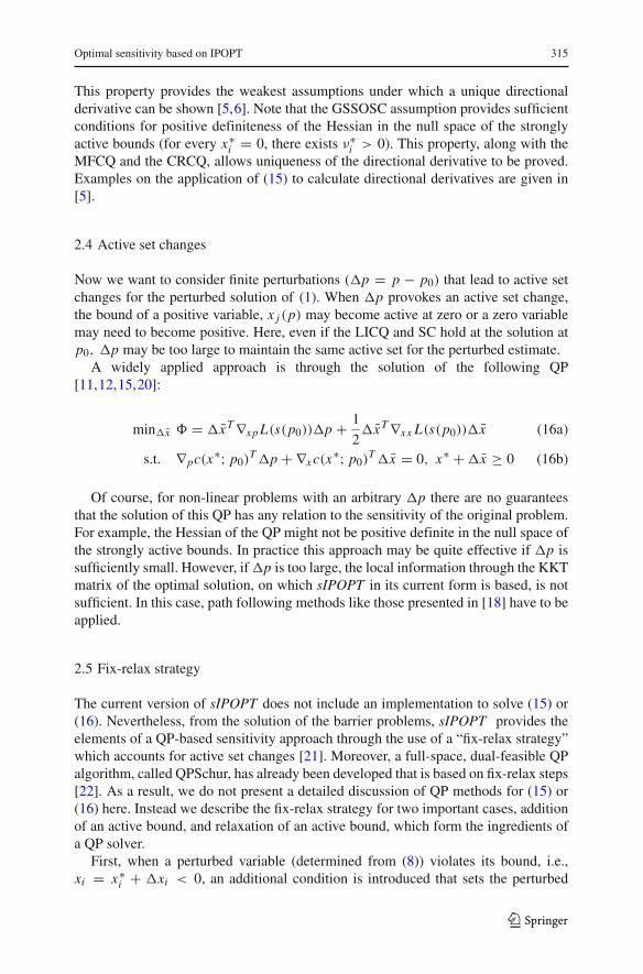
2.4 Active set changes

Now we want to consider finite perturbations (�p = p − p0) that lead to active setchanges for the perturbed solution of (1). When �p provokes an active set change,the bound of a positive variable, x j (p) may become active at zero or a zero variablemay need to become positive. Here, even if the LICQ and SC hold at the solution atp0, �p may be too large to maintain the same active set for the perturbed estimate.

A widely applied approach is through the solution of the following QP[11,12,15,20]:

min�x � = �x T ∇xp L(s(p0))�p + 1

2�x T ∇xx L(s(p0))�x (16a)

s.t. ∇pc(x∗; p0)T �p + ∇x c(x∗; p0)

T �x = 0, x∗ + �x ≥ 0 (16b)

Of course, for non-linear problems with an arbitrary �p there are no guaranteesthat the solution of this QP has any relation to the sensitivity of the original problem.For example, the Hessian of the QP might not be positive definite in the null space ofthe strongly active bounds. In practice this approach may be quite effective if �p issufficiently small. However, if �p is too large, the local information through the KKTmatrix of the optimal solution, on which sIPOPT in its current form is based, is notsufficient. In this case, path following methods like those presented in [18] have to beapplied.

2.5 Fix-relax strategy

The current version of sIPOPT does not include an implementation to solve (15) or(16). Nevertheless, from the solution of the barrier problems, sIPOPT provides theelements of a QP-based sensitivity approach through the use of a “fix-relax strategy”which accounts for active set changes [21]. Moreover, a full-space, dual-feasible QPalgorithm, called QPSchur, has already been developed that is based on fix-relax steps[22]. As a result, we do not present a detailed discussion of QP methods for (15) or(16) here. Instead we describe the fix-relax strategy for two important cases, additionof an active bound, and relaxation of an active bound, which form the ingredients ofa QP solver.

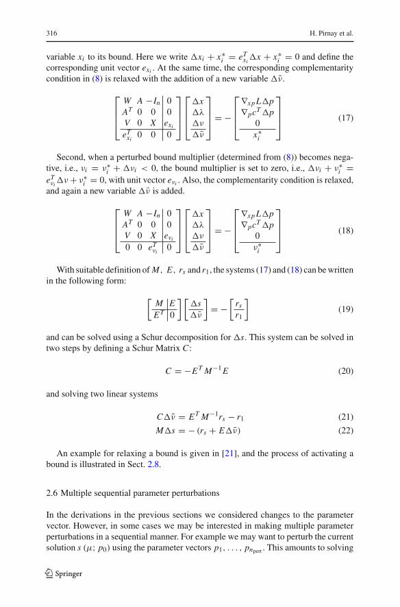
First, when a perturbed variable (determined from (8)) violates its bound, i.e.,xi = x∗

i + �xi < 0, an additional condition is introduced that sets the perturbed

123


variable xi to its bound. Here we write �xi + x∗i = eT

xi�x + x∗

i = 0 and define thecorresponding unit vector exi . At the same time, the corresponding complementaritycondition in (8) is relaxed with the addition of a new variable �ν.

⎡

⎢⎢⎣

W A −In 0AT 0 0 0V 0 X exi

eTxi

0 0 0

⎤

⎥⎥⎦

⎡

⎢⎢⎣

�x�λ

�ν

�ν

⎤

⎥⎥⎦ = −

⎡

⎢⎢⎣

∇xp L�p∇pcT �p

0x∗

i

⎤

⎥⎥⎦ (17)

Second, when a perturbed bound multiplier (determined from (8)) becomes nega-tive, i.e., νi = ν∗

i + �νi < 0, the bound multiplier is set to zero, i.e., �νi + ν∗i =

eTνi

�ν + ν∗i = 0, with unit vector eνi . Also, the complementarity condition is relaxed,

and again a new variable �ν is added.

⎡

⎢⎢⎣

W A −In 0AT 0 0 0V 0 X eνi

0 0 eTνi

0

⎤

⎥⎥⎦

⎡

⎢⎢⎣

�x�λ

�ν

�ν

⎤

⎥⎥⎦ = −

⎡

⎢⎢⎣

∇xp L�p∇pcT �p

0ν∗

i

⎤

⎥⎥⎦ (18)

With suitable definition of M, E, rs and r1, the systems (17) and (18) can be writtenin the following form:

[M EET 0

] [�s�ν

]= −

[rs

r1

](19)

and can be solved using a Schur decomposition for �s. This system can be solved intwo steps by defining a Schur Matrix C :

C = −ET M−1 E (20)

and solving two linear systems

C�ν = ET M−1rs − r1 (21)

M�s = − (rs + E�ν) (22)

An example for relaxing a bound is given in [21], and the process of activating abound is illustrated in Sect. 2.8.

2.6 Multiple sequential parameter perturbations

In the derivations in the previous sections we considered changes to the parametervector. However, in some cases we may be interested in making multiple parameterperturbations in a sequential manner. For example we may want to perturb the currentsolution s (μ; p0) using the parameter vectors p1, . . . , pnpert . This amounts to solving

123


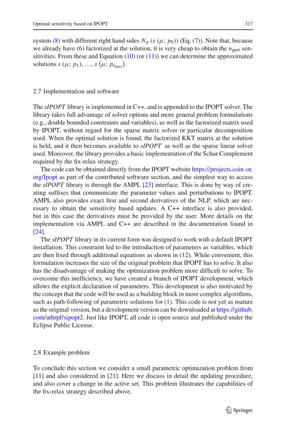
system (8) with different right hand sides Np (s (μ; p0)) (Eq. (7)). Note that, becausewe already have (6) factorized at the solution, it is very cheap to obtain the npert sen-sitivities. From these and Equation (10) (or (11)) we can determine the approximatedsolutions s (μ; p1), …, s

(μ; pnpert

).

2.7 Implementation and software

The sIPOPT library is implemented in C++, and is appended to the IPOPT solver. Thelibrary takes full advantage of solver options and more general problem formulations(e.g., double bounded constraints and variables), as well as the factorized matrix usedby IPOPT, without regard for the sparse matrix solver or particular decompositionused. When the optimal solution is found, the factorized KKT matrix at the solutionis held, and it then becomes available to sIPOPT as well as the sparse linear solverused. Moreover, the library provides a basic implementation of the Schur Complementrequired by the fix-relax strategy.

The code can be obtained directly from the IPOPT website https://projects.coin-or.org/Ipopt as part of the contributed software section, and the simplest way to accessthe sIPOPT library is through the AMPL [23] interface. This is done by way of cre-ating suffixes that communicate the parameter values and perturbations to IPOPT.AMPL also provides exact first and second derivatives of the NLP, which are nec-essary to obtain the sensitivity based updates. A C++ interface is also provided,but in this case the derivatives must be provided by the user. More details on theimplementation via AMPL and C++ are described in the documentation found in[24].

The sIPOPT library in its current form was designed to work with a default IPOPTinstallation. This constraint led to the introduction of parameters as variables, whichare then fixed through additional equations as shown in (12). While convenient, thisformulation increases the size of the original problem that IPOPT has to solve. It alsohas the disadvantage of making the optimization problem more difficult to solve. Toovercome this inefficiency, we have created a branch of IPOPT development, whichallows the explicit declaration of parameters. This development is also motivated bythe concept that the code will be used as a building block in more complex algorithms,such as path-following of parametric solutions for (1). This code is not yet as matureas the original version, but a development version can be downloaded at https://github.com/athrpf/sipopt2. Just like IPOPT, all code is open source and published under theEclipse Public License.

2.8 Example problem

To conclude this section we consider a small parametric optimization problem from[11] and also considered in [21]. Here we discuss in detail the updating procedure,and also cover a change in the active set. This problem illustrates the capabilities ofthe fix-relax strategy described above.

123

https://projects.coin-or.org/Ipopt


https://github.com/athrpf/sipopt2

https://github.com/athrpf/sipopt2


Consider the parametric programming problem:

min x21 + x2

2 + x23 (23)

s.t. 6x1 + 3x2 + 2x3 − p1 = 0

p2x1 + x2 − x3 − 1 = 0

x1, x2, x3 ≥ 0,

with variables x1, x2, and x3 and parameters p1, and p2. As programmed, the IPOPTcode does not distinguish variables from parameters, but the problem can be reformu-lated as (12) by introducing equations that fix the parameters p1, p2 to their nominalvalues p1,a, p2,a .

min x21 + x2

2 + x23 (24a)

s.t. 6x1 + 3x2 + 2x3 − p1 = 0 (24b)

p2x1 + x2 − x3 − 1 = 0 (24c)

p1 = p1,a (24d)

p2 = p2,a (24e)

x1, x2, x3 ≥ 0. (24f)

The KKT conditions for this problem are

2x1 + 6λ1 + p2λ2 − ν1 = 0 (25a)

2x2 + 3λ1 + λ2 − ν2 = 0 (25b)

2x3 + 2λ1 − λ2 − ν3 = 0 (25c)

−λ1 + λ3 = 0 (25d)

λ2x1 + λ4 = 0 (25e)

6x1 + 3x2 + 2x3 − p1 = 0 (25f)

p2x1 + x2 − x3 − 1 = 0 (25g)

p1 − p1,a = 0 (25h)

p2 − p2,a = 0 (25i)

ν1x1 − μ = 0 (25j)

ν2x2 − μ = 0 (25k)

ν3x3 − μ = 0 (25l)

x1, x2, x3, ν1, ν2, ν3 ≥ 0. (25m)

123


The corresponding Newton step is

⎡

⎢⎢⎢⎢⎢⎢⎢⎢⎢⎢⎢⎢⎢⎢⎢⎢⎢⎢⎣

2 λ2 6 p2 −12 3 1 −1

2 2 −1 −1−1 1

λ2 x1 16 3 2 −1p2 1 −1 x1ν1 x1

ν2 x2ν3 x3

11

⎤

⎥⎥⎥⎥⎥⎥⎥⎥⎥⎥⎥⎥⎥⎥⎥⎥⎥⎥⎦

⎡

⎢⎢⎢⎢⎢⎢⎢⎢⎢⎢⎢⎢⎢⎢⎢⎢⎢⎢⎣

�x1�x2�x3�p1�p2�λ1�λ2�ν1�ν2�ν3�λ3�λ4

⎤

⎥⎥⎥⎥⎥⎥⎥⎥⎥⎥⎥⎥⎥⎥⎥⎥⎥⎥⎦

= −

⎡

⎢⎢⎢⎢⎢⎢⎢⎢⎢⎢⎢⎢⎢⎢⎢⎢⎢⎢⎢⎢⎢⎣

2x∗1 + 6λ∗

1 + p2λ∗2 − ν∗

1

2x∗2 + 3λ∗

1 + λ∗2 − ν∗

2

2x∗3 + 2λ∗

1 − λ∗2 − ν∗

3

−λ∗1 + λ∗

3

λ∗2x∗

1 + λ∗4

6x∗1 + 3x∗

2 + 2x∗3 − p∗

1

p∗2 x∗

1 + x∗2 − x∗

3 − 1

ν∗1 x∗

1 − μ

ν∗2 x∗

2 − μ

ν∗3 x∗

3 − μ

p∗1 − p1,a

p∗2 − p2,a

⎤

⎥⎥⎥⎥⎥⎥⎥⎥⎥⎥⎥⎥⎥⎥⎥⎥⎥⎥⎥⎥⎥⎦

(26)

where the right hand side is zero at the solution (note that the ordering of the variablesis now as in Eq. (14)). Also, note that this Newton step can easily be transformedinto (14) by rearranging rows and columns. Now consider the exact solutions of twoneighboring parameter sets pa = [

p1,a, p2,a] = [5, 1] and pb = [4.5, 1]. Using

the “bound relax” option in IPOPT to satisfy bounds exactly, the corresponding NLPsolutions are

s(pa)= [0.6327, 0.3878, 0.0204, 5, 1, | − 0.1633,−0.2857, |0, 0, 0, | − 0.1633, 0.1808] ,

and

s(pb) = [0.5, 0.5, 0, 4.5, 1, |0,−1, |0, 0, 1, |0, 0.5] .

Clearly, there is a change in the active set, when changing the parameters from pa

to pb. This is easily verified from the decrease of x3 to zero. When using pb the boundis active, while it is inactive when the parameters are set to pa . This change in theactive set is not captured by the linearization of the KKT conditions. For example,

123


using (10) would require that we first solve the linear system (9), and use the solutionto update the values of the variables. In this example we would solve the linear system

⎡

⎢⎢⎢⎢⎢⎢⎢⎢⎢⎢⎢⎢⎢⎢⎢⎢⎢⎢⎣

2 λ2 6 p2 −12 3 1 −1

2 2 −1 −1−1 1

λ2 x1 16 3 2 −1p2 1 −1 x1ν1 x1

ν2 x2ν3 x3

11

⎤

⎥⎥⎥⎥⎥⎥⎥⎥⎥⎥⎥⎥⎥⎥⎥⎥⎥⎥⎦

⎡

⎢⎢⎢⎢⎢⎢⎢⎢⎢⎢⎢⎢⎢⎢⎢⎢⎢⎢⎣

�x1�x2�x3�p1�p2�λ1�λ2�ν1�ν2�ν3�λ3�λ4

⎤

⎥⎥⎥⎥⎥⎥⎥⎥⎥⎥⎥⎥⎥⎥⎥⎥⎥⎥⎦

= −

⎡

⎢⎢⎢⎢⎢⎢⎢⎢⎢⎢⎢⎢⎢⎢⎢⎢⎢⎢⎣

0000000000

�p10

⎤

⎥⎥⎥⎥⎥⎥⎥⎥⎥⎥⎥⎥⎥⎥⎥⎥⎥⎥⎦

, (27)

where �p1 = p1,a − p1,b = 5 − 4.5. This Newton step yields an updated iterate of

s(pb) = [0.5765, 0.3775,−0.0459, 4.5, 1, | − 0.1327,

−0.3571, |0, 0, 0, | − 0.1327, 0.2099] + o(‖�p‖) (28)

which violates the bounds on x3. On the other hand, taking into consideration theactive set change, we use (17) and augment the KKT system fixing the variable to thebound, and relaxing the complementarity condition. The Newton step now becomes:

⎡

⎢⎢⎢⎢⎢⎢⎢⎢⎢⎢⎢⎢⎢⎢⎢⎢⎢⎢⎢⎢⎣

2 λ2 6 p2 −12 3 1 −1

2 2 −1 −1−1 1

λ2 x1 16 3 2 −1p2 1 −1 x1ν1 x1

ν2 x2ν3 x3 1

11

1

⎤

⎥⎥⎥⎥⎥⎥⎥⎥⎥⎥⎥⎥⎥⎥⎥⎥⎥⎥⎥⎥⎦

⎡

⎢⎢⎢⎢⎢⎢⎢⎢⎢⎢⎢⎢⎢⎢⎢⎢⎢⎢⎢⎢⎣

�x1�x2�x3�p1�p2�λ1�λ2�ν1�ν2�ν3�λ3�λ4

�ν3

⎤

⎥⎥⎥⎥⎥⎥⎥⎥⎥⎥⎥⎥⎥⎥⎥⎥⎥⎥⎥⎥⎦

= −

⎡

⎢⎢⎢⎢⎢⎢⎢⎢⎢⎢⎢⎢⎢⎢⎢⎢⎢⎢⎢⎢⎣

0000000000

δp10x∗

3

⎤

⎥⎥⎥⎥⎥⎥⎥⎥⎥⎥⎥⎥⎥⎥⎥⎥⎥⎥⎥⎥⎦

, (29)

which yields an updated iterate of

s(pb) = [0.5, 0.5, 0, 4.5, 1, |0,−1, |0, 0, 0, |0, 0.5948] + o(‖�p‖), (30)

and this is a very good approximation to the optimal solution to the problem withproblem data pb. Some differences are expected for the linear system, as λ4, x1 andλ2 appear in the nonlinear constraint (25e) in the KKT conditions.

123


3 Advanced step NMPC

In this section we describe the advanced step nonlinear model predictive control (as-NMPC) strategy that makes direct use of IPOPT coupled with the sensitivity code,sIPOPT. Following a brief description of this strategy, we apply the advanced stepcontrol scheme to the continuous stirred tank reactor (CSTR) model proposed by [25].A similar case study was used by [21] to illustrate stability and optimality results forsensitivity based NMPC. In addition, we then consider a large-scale case study wherea distillation column is modeled.

In this section we assume that the dynamics of the plant can be described with thefollowing discrete time dynamic model

zk+1 = f (zk, uk) , (31)

with initial condition z0, and where zk ∈ RNz are the state variables and uk ∈ R

Nu

are the control inputs. In order to drive the system to a desired operating conditionwe solve a dynamic optimization problem that generates the needed optimal inputtrajectory. The NMPC formulation used here solves a dynamic optimization problemover a predictive horizon of the following form:

minN∑

l=0

(zl − zl

)TP

(zl − zl

) +N−2∑

l=0

(ul − ul+1)T Q (ul − ul+1) (32a)

s.t. zl+1 = f (zl , ul) ∀ l = 0, . . . , N − 1 (32b)

z0 = z(k) (32c)

zl ∈ X, ul ∈ U, (32d)

where z is the desired value of the state and P and Q are diagonal positive definiteweight matrices of appropriate dimensions. Also, we have considered a zero orderhold on the inputs, that is the input variables are constant at each sampling time.

At the kth sampling time, after the actual state of the system (z(k)) is obtained (orestimated), we solve problem (32) using this state as the initial condition (z0 = z(k)).This generates the optimal control trajectory for the predictive time horizon. Fromthis, we take the value from the first sampling time, u0, and inject it into the plant asthe actual input, u(k). Once the plant reaches the next sampling time the NLP is solvedagain, with the initial condition set to the current state of the system. However, by thetime we obtain the next NLP solution the plant has moved away from z(k). This com-putational delay could potentially destabilize the system, and this motivates the needfor faster NMPC methods that generate the input online with as little delay as possible.

To address this issue Advanced Step NMPC was proposed in [16]. At samplingtime k − 1, this strategy generates a prediction of the state of the system at time k(i.e., z1 from (32b)) using the injected input, u(k − 1) and the model of the plant.The prediction z1 is used instead of z(k) as the initial condition of the plant in theNLP (32), and an approximate problem is solved in background between samplingtimes. Once the new state of the system is measured or estimated at sampling time

123


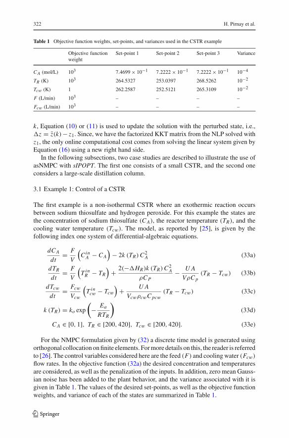
Table 1 Objective function weights, set-points, and variances used in the CSTR example

Objective functionweight

Set-point 1 Set-point 2 Set-point 3 Variance

CA (mol/L) 103 7.4699 × 10−1 7.2222 × 10−1 7.2222 × 10−1 10−4

TR (K) 103 264.5327 253.0397 268.5262 10−2

Tcw (K) 1 262.2587 252.5121 265.3109 10−2

F (L/min) 103 – – – –

Fcw (L/min) 103 – – – –

k, Equation (10) or (11) is used to update the solution with the perturbed state, i.e.,�z = z(k)− z1. Since, we have the factorized KKT matrix from the NLP solved withz1, the only online computational cost comes from solving the linear system given byEquation (16) using a new right hand side.

In the following subsections, two case studies are described to illustrate the use ofasNMPC with sIPOPT. The first one consists of a small CSTR, and the second oneconsiders a large-scale distillation column.

3.1 Example 1: Control of a CSTR

The first example is a non-isothermal CSTR where an exothermic reaction occursbetween sodium thiosulfate and hydrogen peroxide. For this example the states arethe concentration of sodium thiosulfate (CA), the reactor temperature (TR), and thecooling water temperature (Tcw). The model, as reported by [25], is given by thefollowing index one system of differential-algebraic equations.

dCA

dt= F

V

(Cin

A − CA

)− 2k (TR) C2

A (33a)

dTR

dt= F

V

(T in

R − TR

)+ 2(−�HR)k (TR) C2

A

ρCP− U A

VρC p(TR − Tcw) (33b)

dTcw

dt= Fcw

Vcw

(T in

cw − Tcw

)+ U A

VcwρcwC pcw(TR − Tcw) (33c)

k (TR) = ko exp

(− Ea

RTR

)(33d)

CA ∈ [0, 1], TR ∈ [200, 420], Tcw ∈ [200, 420]. (33e)

For the NMPC formulation given by (32) a discrete time model is generated usingorthogonal collocation on finite elements. For more details on this, the reader is referredto [26]. The control variables considered here are the feed (F) and cooling water (Fcw)

flow rates. In the objective function (32a) the desired concentration and temperaturesare considered, as well as the penalization of the inputs. In addition, zero mean Gauss-ian noise has been added to the plant behavior, and the variance associated with it isgiven in Table 1. The values of the desired set-points, as well as the objective functionweights, and variance of each of the states are summarized in Table 1.

123


0 200 400 600 800 1000 12000.72

0.725

0.73

0.735

0.74

0.745

0.75

0.755

time [min]

CA [m

ol/L

]

Set pointNMPC

i

asNMPC

(a)

0 200 400 600 800 1000 1200252

254

256

258

260

262

264

266

268

270

time [min]

T [K

]

Set pointNMPC

i

asNMPC

(b)

0 200 400 600 800 1000 1200252

254

256

258

260

262

264

266

time [min]

Tj [K

] Set pointNMPC

i

asNMPC

(c)

0 200 400 600 800 1000 12000

10

20

30

F [L

/min

]

NMPCi

asNMPC

0 200 400 600 800 1000 12000

50

100

150

200

time [min]

Fcw

[L/m

in]

(d)

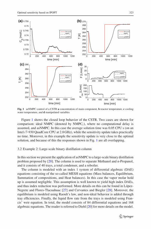
Fig. 1 asNMPC control of a CSTR a concentration of main component, b reactor temperature, c coolingwater temperature, and d manipulated variables

Figure 1 shows the closed loop behavior of the CSTR. Two cases are shown forcomparison: ideal NMPC (denoted by NMPCi ), where no computational delay isassumed, and asNMPC. In this case the average solution time was 0.05 CPU s (on anIntel i7-930 QuadCore CPU at 2.8 GHz), while the sensitivity update takes practicallyno time. Moreover, in this example the sensitivity update is very close to the optimalsolution, and because of this the responses shown in Fig. 1 are all overlapping.

3.2 Example 2: Large-scale binary distillation column

In this section we present the application of asNMPC to a large-scale binary distillationproblem proposed by [20]. The column is used to separate Methanol and n-Propanol,and it consists of 40 trays, a total condenser, and a reboiler.

The column is modeled with an index 1 system of differential algebraic (DAE)equations consisting of the so-called MESH equations (Mass balances, Equilibrium,Summation of compositions, and Heat balances). In this case the vapor molar holdup is assumed negligible. This assumption is well known to yield high index DAEs,and thus index reduction was performed. More details on this can be found in López-Negrete and Flores-Tlacuahuac [27] and Cervantes and Biegler [28]. Moreover, theequilibrium is modeled using Raoult’s law, and non-ideal behavior is added throughtray efficiencies. Finally, the liquid flow rate from the trays is modeled using Fran-cis’ weir equation. In total, the model consists of 84 differential equations and 168algebraic equations. The reader is referred to Diehl [20] for more details on the model.

123


Table 2 Set-point information and objective function weights for the distillation column example

Objective function weight Set-point 1 Set-point 2

T14 (K) 104 351.0321 356.6504

T28 (K) 104 337.4470 346.9235

D (mol/s) 10−1 1.1152 18.3859

QC (J) 10−1 8.9955 × 105 1.6221 × 106

R (–) 102 – –

Q R (K) 102 – –

For this example we considered 60 s sampling times, and 10 sampling times in thepredictive horizon. As described in the CSTR example, the continuous time model istransformed into a discrete time model using collocation. Thus, using 3 point Radaucollocation, the NLP consists of 19,814 variables and 19,794 equality constraints. Toaccount for plant model mismatch we added noise to the differential variables (totalmolar holdup and liquid compositions at each tray). The noise was assumed uncorre-lated, zero mean and Gaussian with variance 10−4 for the holdups and 10−6 for thecompositions.

The control variables of this problem are the reboiler heat Q R and the reflux rate ofthe top product R. In the objective function for the NLP we consider only temperaturesfrom trays 14 and 28, since they are much more sensitive to changes than the head andbottom product streams. We also include the distillate flow rate and condenser heatduty in the objective. Note that we have numbered the trays from top to bottom. Also,we consider the penalization to changes in the inputs. Finally, set-point informationand objective function weights are summarized in Table 2.

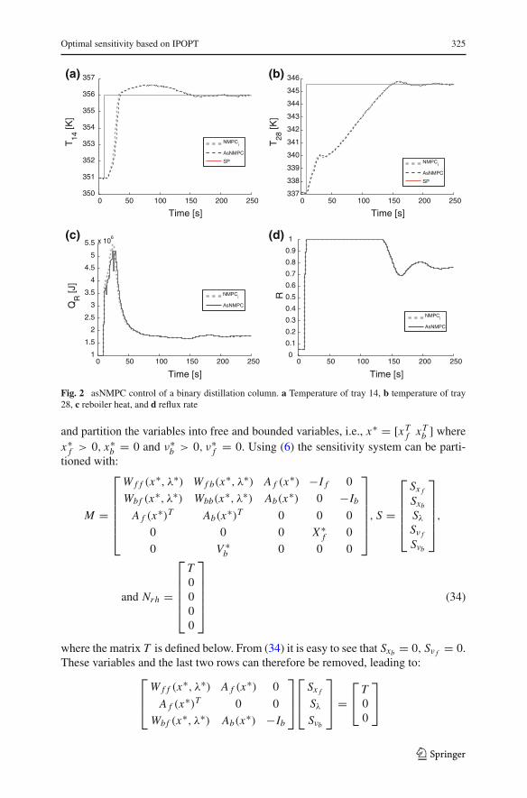
Figure 2 shows the simulation results comparing the advanced step NMPC with theideal case. The average solution time of the NLP was 9.4 CPU s. Both the ideal andadvanced step NMPC strategies were able to perform the set-point change. However,the latter adds practically no computational delays, and this is important for real timeoptimization schemes.

4 Parameter estimation

In this last section, we consider the capabilities of sIPOPT for recovery of reducedHessian information, and this is of particular importance for parameter estimationproblems to estimate the covariance of the calculated parameters. We begin with theextraction of reduced Hessian information from the solution of (1) with IPOPT. Fol-lowing this, we consider the parameter estimation problem directly.

4.1 Extraction of reduced Hessian information

An important byproduct of the sensitivity calculation is information related to theHessian of the Lagrange function pertinent to the second-order conditions. At thesolution of (1) we consider a sensitivity system, M S = Nrh , with M defined in (6),

123


0 50 100 150 200 250350

351

352

353

354

355

356

357

Time [s]

T14

[K]

NMPCi

AsNMPC

SP

(a)

0 50 100 150 200 250337

338

339

340

341

342

343

344

345

346

Time [s]

T28

[K]

NMPCi

AsNMPC

SP

(b)

0 50 100 150 200 2501

1.5

2

2.5

3

3.5

4

4.5

5

5.5 x 106

Time [s]

QR

[J]

NMPCi

AsNMPC

(c)

0 50 100 150 200 2500

0.1

0.2

0.3

0.4

0.5

0.6

0.7

0.8

0.9

1

Time [s]

R

NMPCi

AsNMPC

(d)

Fig. 2 asNMPC control of a binary distillation column. a Temperature of tray 14, b temperature of tray28, c reboiler heat, and d reflux rate

and partition the variables into free and bounded variables, i.e., x∗ = [xTf xT

b ] wherex∗

f > 0, x∗b = 0 and ν∗

b > 0, ν∗f = 0. Using (6) the sensitivity system can be parti-

tioned with:

M =

⎡

⎢⎢⎢⎢⎢⎣

W f f (x∗, λ∗) W f b(x∗, λ∗) A f (x∗) −I f 0

Wbf (x∗, λ∗) Wbb(x∗, λ∗) Ab(x∗) 0 −Ib

A f (x∗)T Ab(x∗)T 0 0 0

0 0 0 X∗f 0

0 V ∗b 0 0 0

⎤

⎥⎥⎥⎥⎥⎦, S =

⎡

⎢⎢⎢⎢⎣

Sx f

Sxb

Sλ

Sν f

Sνb

⎤

⎥⎥⎥⎥⎦,

and Nrh =

⎡

⎢⎢⎢⎢⎣

T0000

⎤

⎥⎥⎥⎥⎦(34)

where the matrix T is defined below. From (34) it is easy to see that Sxb = 0, Sν f = 0.These variables and the last two rows can therefore be removed, leading to:

⎡

⎢⎣W f f (x∗, λ∗) A f (x∗) 0

A f (x∗)T 0 0

Wbf (x∗, λ∗) Ab(x∗) −Ib

⎤

⎥⎦

⎡

⎢⎣Sx f

Sλ

Sνb

⎤

⎥⎦ =⎡

⎣T00

⎤

⎦

123


We now define Sx f = Z SZ + Y SY , with A f (x∗)T Z = 0, and A f (x∗)T Y and

R = [Y | Z ] nonsingular. Here, we choose Z and Y by partitioning xTf = [xT

D xTI ]

with dependent and independent variables xD ∈ Rm, xI ∈ R

nI , so that ATf =

[ATD | AT

I ], with AD square and nonsingular. This leads to Y T = [Im | 0], Z T =[−AI (AD)−1 | InI ].

Using the linear transformation, H T M H S = H T Nrh with H =⎡

⎣R 0 00 I 00 0 I

⎤

⎦ and

S = H−1S leads to:⎡

⎢⎢⎢⎣

Y T W f f (x∗, λ∗)Y Y T W f f (x∗, λ∗)Z Y T A f (x∗) 0

Z T W f f (x∗, λ∗)Y Z T W f f (x∗, λ∗)Z 0 0

A f (x∗)T Y 0 0 0

Wbf (x∗, λ∗)Y Wbf (x∗, λ∗)Z Ab(x∗) −Ib

⎤

⎥⎥⎥⎦

⎡

⎢⎢⎢⎣

SY

SZ

Sλ

Sνb

⎤

⎥⎥⎥⎦ =

⎡

⎢⎢⎢⎣

Y T T

Z T T

0

0

⎤

⎥⎥⎥⎦.

(35)

From (35) we have SY = 0 and SZ = (Z T W f f Z)−1 Z T T . Choosing Z T T = I revealsSZ as the inverse of the reduced Hessian matrix HR = Z T W f f Z .

Note that the transformation of the sensitivity system (35) need not be implemented.Instead, for a chosen set of nI ≤ nx − m independent variables, AD nonsingular,T T = [0 | InI ] and the matrices defined in (34), the reduced Hessian can be founddirectly by solving M S = Nrh . From the choice of Z , S f = Z SZ and SZ = HR ,the reduced Hessian can be extracted easily from the rows of S. In the next section wewill see that this property provides an efficient approach to extract an estimate of thecovariance matrix for parameter estimation problems.

4.2 Reduced Hessian/Covariance relation

Consider the parameter estimation problem given by:

minθ,γ,y1

2

[(y − y)T V −1

y (y − y) + (θ − θ )T V −1θ (θ − θ )

](36a)

s.t. c(θ, γ, y) = 0 (36b)

where we define the variables x = [θT , γ T , yT ]T , y are state variables and θ andγ represent estimated parameters with and without prior measurement information,respectively. Measurements for the state variables y and parameters θ are denoted byy and θ , respectively, and covariance of these measurements is given by Vy and Vθ ,respectively. KKT conditions for (36) are given by:

V −1y (y∗ − y) + ∇yc(x∗)λ∗ = 0 (37a)

V −1θ (θ∗ − y) + ∇θc(x∗)λ∗ = 0 (37b)

∇γ c(x∗)λ∗ = 0 (37c)

c(x∗) = 0 (37d)

123


As inequality constraints do not appear, problem (36) is a simplification of (1). Con-sequently, the set of bounded variables described in Sect. 4.1 is empty and the system(35) is simplified. Also, from (37a) to (37c) and from the LICQ assumption we defineλ∗ as:

λ∗ = −(AT A)−1 A

⎡

⎢⎣V −1

y (y∗ − y)

V −1θ (θ∗ − θ )

0

⎤

⎥⎦ (38)

where A = ∇c(x∗). For suitable maximum likelihood assumptions on (36),

E[y∗ − y

] = 0, E

[θ∗ − θ

]= 0, Equation (38) leads to E

[λ∗] = 0.

Using the multiplier estimate λ∗ = 0 we now consider the sensitivity of x∗ toperturbations of the data, δ y and δθ . Application of IFT to (37), as in (8) leads to thefollowing sensitivity system:

⎡

⎢⎢⎣

V −1θ 0 0 Aθ

0 0 0 Aγ

0 0 V −1y Ay

ATθ AT

γ ATy 0

⎤

⎥⎥⎦

⎡

⎢⎢⎣

δθ

δγ

δyδλ

⎤

⎥⎥⎦ =

⎡

⎢⎢⎣

V −1θ δθ

0V −1

y δ y0

⎤

⎥⎥⎦ . (39)

where AT = [ATθ |AT

γ |ATy |0], and we assume that Ay is nonsingular. From

AT δx = ATθ δθ + AT

γ δγ + ATy δy = 0 (40)

we can define δy = −A−Ty (AT

θ δθ + ATγ γ ), and δx = Z

[δθ

δγ

], with AT Z = 0 and

the choice:

Z =⎡

⎣I 00 I

−A−Ty AT

θ −A−Ty AT

γ

⎤

⎦.

Substituting δx into (39) leads to:

⎛

⎝Z T

⎡

⎣V −1

θ 0 00 0 00 0 V −1

y

⎤

⎦Z

⎞

⎠[

δθ

δγ

]= Z T

⎡

⎣V −1

θ δθ

0V −1

y δ y

⎤

⎦, (41)

where the matrix on the left hand side is the reduced Hessian, HR . Solving for δθ andδγ leads to:

[δθ

δγ

]= H−1

R

[V −1

θ δθ − Aθ A−1y V −1

y δ y

−Aγ A−1y V −1

y δ y

]. (42)

123


We can now recover the covariance for the parameters δθ and δγ by noting the fol-

lowing expected values: Vy = E[δ y δ yT

], Vθ = E

[δθ δθT

], and E

[δ y δθT

]= 0.

Taking expected values of

[δθ

δγ

][δθT δγ T ], using (42), and simplifying the matrix

algebra, leads to:

E

{[δθ

δγ

] [δθT δγ T

]}= Vθ,γ = H−1

R . (43)

Consequently, finding the inverse of the reduced Hessian, as described in Sect. 4.1directly determines an estimate of the covariance matrix for the parameter estimates.

4.3 Parameter estimation case study

To illustrate the approximation of the covariance using (35) and (43), we again con-sider the CSTR model described in equations (33a)–(33c). For this case study, wegenerated 14 datasets that were corrupted with Gaussian noise. These were then usedto estimate two parameters, θ = [�HR, U A] the heat of reaction and the heat trans-fer coefficient multiplied by the area of the reactor, respectively. The values of theseparameters used in the simulation to generate data were −�HR = 5.9662×105 J/moland U A = 1.2 × 106 J/min · K. The parameters were estimated by solving the leastsquares problem, and gradually increasing the number of data sets used. The leastsquares problem has the following form:

minθ

� = 1

2

Nd∑

j=1

N∑

l=0

(yl, j − yl, j

)TV −1

y

(yl, j − yl, j

)(44a)

s.t. zl+1, j = f(zl, j , ul, j , θ

) ∀ l = 0, . . . , N − 1, j = 1, . . . , Nd (44b)

yl, j = g(zl, j

)(44c)

z0, j = z(0, j) (44d)

zl, j ∈ X, ul, j ∈ U, yl, j ∈ Y, (44e)

where Nd is the number of datasets, θ represents the parameters (in this case timeindependent), equation (44c) represents the model prediction of the measurement,Vy = diag

(10−4, 10−2, 10−2

)is the covariance matrix associated with the measure-

ments, and yl are the measurements. For this example we consider that g (zl) = zl ,i.e., all three states were measured.

Having the covariance of the estimates allows us to quantify their reliability byanalyzing the confidence region. Thus, following [29], we consider the Taylor seriesexpansion of the objective function (44a)

1

2

(θ − θ∗)T

V −1θ

(θ − θ∗) ≈ �(θ) − �(θ∗) ≤ c. (45)

123


Table 3 Estimated parameters and the calculated standard deviation

Number of datasets −�HR (J/mol) σ−�HR (J/mol) UA (J/min K) σUA (J/min K)

2 6.0480 × 105 8.4236 × 102 1.2248 × 106 1.1067 × 103

4 6.0851 × 105 5.9101 × 102 1.2297 × 106 1.1089 × 103

8 6.1762 × 105 4.1208 × 102 1.2529 × 106 1.1193 × 103

14 6.3153 × 105 3.0222 × 102 1.2835 × 106 1.1329 × 103

−2000 −1500 −1000 −500 0 500 1000 1500 2000

−1

−0.5

0

0.5

1

x 104

(Δ HR

− Δ HR∗ )

(UA

− U

A∗ )

4

8

14

2

Fig. 3 Error ellipses for the estimated parameters, for when 2, 4, 8, and 14 datasets are used

This allows us to construct level sets of the objective function for increasing valuesof c. These ellipsoids are defined by the covariance of the estimated parameters. More-over, it can be shown that, for large numbers of datasets with independent Gaussianmeasurement errors with known covariance Vy , then c is determined for the confidencelevel, β of a chi-square distribution χ2 (nθ , β), where nθ is the number of degrees offreedom.

Equation (45) allows us to get order-of-magnitude estimates of the parameter con-fidence levels under different scenarios of practical interest. However, this inferenceanalysis only applies to standard least squares formulations.

Table 3 shows the estimated parameters and the variance associated with them.Here we see that there is good agreement between the estimated parameters and theones used for generating the datasets. Moreover, we can also note that the standarddeviation of the estimates improves as more data are used. Figure 3 shows the 95 %confidence ellipsoids for the estimated parameters. The largest of these is for the casewhen only two datasets are used, the second largest for four datasets, and the inner-most ellipse when 14 datasets are used. This figure shows clearly that as more dataare used, the confidence region shrinks, and therefore our estimated parameters haveless variance.

123


5 Conclusions

Sensitivity analysis is an essential component of any optimization study. It providesinformation on regularity and curvature conditions at KKT points and provides first-order estimates of the minimizer to parametric variations in nonlinear programs. Withthe availability of fast large-scale nonlinear programming solvers, it is also possibleto integrate sensitivity capabilities to these solvers. This study discusses the develop-ment of sIPOPT , a program for NLP sensitivity that is paired with the IPOPT solver.Here we review properties of barrier methods and sensitivity analysis derived from theimplicit function theorem. These require well-known regularity conditions includingstrict complementarity, strong second-order conditions and LICQ. We also relax thelast condition and extend our method to include a fix-relax strategy, which is usefulto handle active set changes; this is illustrated with a small example.

The sIPOPT program is also demonstrated on three large-scale case studies forreal-time optimization and control. The first two case studies deal with the nonlinearcontrol of chemical process units, where IPOPT solves a nonlinear program in back-ground and sIPOPT provides an estimate of a neighboring solution, with initial statesperturbed by noise or model mismatch. The third case study deals with parameterestimation of a dynamic system solved with IPOPT; this demonstrates how sIPOPTdirectly retrieves the covariance matrix of the estimated parameters (i.e., the reducedHessian) in order to approximate the confidence region.

Written in C++, sIPOPT is an open source code that can be obtained directlyfrom the contributed software section of the IPOPT website, and the simplest way toaccess it is through the AMPL interface. Future extensions to this code will deal withadditional features that rely on Schur complement decompositions, including system-atic treatment of active set changes. This will be especially useful for applications innonlinear state estimation and control, as well as real-time optimization.

References

1. Wächter, A., Biegler, L.T.: On the implementation of a primal-dual interior point filter line searchalgorithm for large-scale nonlinear programming. Math. Program. 106(1), 25–57 (2006)

2. Fiacco, A.V.: Introduction to sensitivity and stability analysis in nonlinear programming. Mathematicsin Science and Engineering, vol. 165. Academic Press, Dublin (1983)

3. Fiacco, A.V., Ishizuka, Y.: Sensitivity and stability analysis for nonlinear programming. Ann. Oper.Res. 27, 215–236 (1990)

4. Büskens, H., Maurer, C. : Sensitivity analysis and real-time control of parametric control problemsusing nonlinear programming methods. In: Grötschel, M., Krumke, S., Rambau, J. (eds.) Online Opti-mization of Large-scale Systems, pp. 57–68. Springer, Berlin (2001)

5. Kyparisis, J.: Sensitivity analysis for nonlinear programs and variational inequalities with nonuniquemultipliers. Math. Oper. Res. 15(2), 286–298 (1990)

6. Kojima, M.: Strongly stable stationary solutions in nonlinear programs. In: Robinson, S.M. (ed.) Anal-ysis and Computation of Fixed Points, pp. 93–138. Academic Press, New York (1980)

7. Kojima, M., Hirabayashi, R.: Continuous deformation of nonlinear programs. Math. Program. Study21, 150–198 (1984)

8. Jongen, H.T., Jonker, P., Twilt, F.: Nonlinear Optimization in Finite Dimensions. Kluwer, Dordrecht(2000)

9. Jongen, H.T., Meer, K., Triesch, E.: Optimization Theory. Kluwer, Dordrecht (2004)

123


10. Fiacco, A.V. Ghaemi, A.: A user’s manual for SENSUMT. A penalty function computer program forsolution, sensitivity analysis and optimal bound value calculation in parametric nonlinear programs.Technical Report T-434, Management Science and Engineering, George Washington University (1980)

11. Ganesh, N., Biegler, L.T.: A reduced hessian strategy for sensitivity analysis of optimal flowsheets.AIChE 33, 282–296 (1987)

12. Wolbert, D., Joulia, X., Koehret, B., Biegler, L.T.: Flowsheet optimization and optimal sensitivityanalysis using exact derivatives. Comput. Chem. Eng. 18, 1083 (1994)

13. Forbes, J., Marlin, T.E.: Design cost: a systematic approach to technology selection for model-basedreal-time optimization systems. Comput. Chem. Eng. 20, 717–734 (1996)

14. Diehl, M., Findeisen, R., Allgöwer, F.: A stabilizing real-time implementation of nonlinear model pre-dictive control. In: Biegler, L.T., Keyes, D., Ghattas, O., van Bloemen Waanders, B., Heinkenschloss,M. (eds.) Real-Time PDE-Constrained Optimization, pp. 25–52. SIAM, Philadelphia (2007)

15. Kadam, J. Marquardt, W.: Sensitivity-based solution updates in closed-loop dynamic optimization. In:Proceedings of the DYCOPS 7 Conference. Elsevier, Amsterdam (2004)

16. Zavala, V.M., Biegler, L.T.: The advanced-step NMPC controller: optimality, stability and robustness.Automatica 45(1), 86–93 (2009)

17. Forsgren, A., Gill, P.E., Wright, M.H.: Interior point methods for nonlinear optimization. SIAM Rev.44(4), 525–597 (2002)

18. Guddat, J., Guerra Vazquez, F., Jongen, H.T.: Parametric Optimization: Singularities, Pathfollowingand Jumps. Teubner, Stuttgart (1990)

19. Robinson, S.M.: Generalized equations and their solutions, part II: applications to nonlinear program-ming. Math. Program. Study 19, 200–221 (1982)

20. Diehl, M.: Real-Time Optimization for Large Scale Nonlinear Processes. Ph.D. thesis, UniversitätHeidelberg (2001). http://www.ub.uni-heidelberg.de/archiv/1659/

21. Zavala, V.M.: Computational Strategies for the Operation of Large-Scale Chemical Processes. Ph.D.thesis, Carnegie Mellon University (2008)

22. Bartlett, R.A., Biegler, L.T.: QPSchur: a dual, active-set, schur-complement method for large-scaleand structured convex quadratic programming. Optim. Eng. 7, 5–32 (2006)

23. Fourer, R., Gay, D.M., Kernighan, B.W.: AMPL: a modeling language for mathematical program-ming. Duxbury Press, Pacific Grove (2002)

24. Pirnay, H., López-Negrete, R., Biegler, L.T.: sIPOPT Reference Manual. Carnegie Mellon University(2011). https://projects.coin-or.org/Ipopt

25. Rajaraman, S., Hahn, J., Mannan, M.S.: A methodology for fault detection, isolation, and identificationfor nonlinear processes with parametric uncertainties. Ind. Eng. Chem. Res. 43(21), 6774–6786 (2004)

26. Biegler, L.T.: Nonlinear Programming: Concepts, Algorithms, and Applications to Chemical Pro-cesses. SIAM, Philadelphia (2010)

27. López-Negrete, R., Flores-Tlacuahuac, A.: Optimal start-up and product transition policies of a reactivedistillation column. Ind. Eng. Chem. Res. 46, 2092–2111 (2007)

28. Cervantes, A.M., Biegler, L.T.: Large-scale DAE optimization using a simultaneous NLP formula-tion. AIChE J. 44(5), 1038–1050 (1998)

29. Bard, Y.: Nonlinear Parameter Estimation. Academic Press, New York (1974)

123

http://www.ub.uni-heidelberg.de/archiv/1659/


Optimal sensitivity based on IPOPT

Documents

Transcript of Optimal sensitivity based on IPOPT