Optimal renting /selling strategies in oligopoly durable goods markets

OPTIMAL RENTING/SELLING STRATERGIES IN OLIGOPOLY DURABLE GOODS MARKETS

by

Golovko Sergiy

A thesis submitted in partial fulfillment of the requirements for the degree of

MA in Economics

Kyiv School of Economics

2010

Thesis Supervisor: Professor Prokopovych Pavlo

Approved by ___________________________________________________

Head of the KSE Defense Committee, Professor Roy Gardner

__________________________________________________

__________________________________________________

__________________________________________________

Date ___________________________________

Kyiv School of Economics

Abstract

OPTIMAL RENTING/SELLING STRATERGIES IN OLIGOPOLY DURABLE GOODS MARKETS

by Golovko Sergiy

Thesis Supervisor: Professor Prokopovych Pavlo

This paper studies a simultaneous-move three-period model in which firms

choose the durability of their goods, whether rent or sell and how much to

produce. We show that a firm’s profitability tends to improve if it lowers

durability of its output. Then we show that the previously known results

regarding commitment to the selling strategy are robust with respect to time if the

firms make their renting/selling decisions at the beginning of each period.

However, if the firms make their renting/selling decisions at the pre-play stage of

the game, they are less likely to commit to the selling strategy, choosing instead

some mix of renting/selling strategies.

If the firms are infinitely lived, they should be more patient to sustain trigger

strategies when the good is less durable. Moreover, analyzing the model under

different specifications of cooperation, we show that the firms should be more

patient when they cooperate both in choosing renting/selling strategies and in

choosing quantities than when they cooperate only in choosing renting/selling

strategies.

TABLE OF CONTENTS

Number Page

Chapter 1 Introduction………………………………………………………..1

Chapter 2 Literature Review…………………………………………………...3

Chapter 3 Two Period-Model, Main Results…………………………………...8

Chapter 4 Three Period Model……………….………………………………11

4.1 The Case of Two-Period Durability…………….…….…..……11

4.2 The Case of Three-Period Durability …..………….……..……24

4.3 The Case of Asymmetric Durability …..............…………..……29

4.4 Choice of Durability ….……………..….……………….……32

4.5 The Case of Two-Period Durability……...……………………33

Chapter 5 Repeated Interaction Model………………………………………36

Chapter 6 Conclusions………………………………………………………44

Works Cited…………………………………………………………………46

ii

LIST OF TABLES

Number Page

Table 1 Total Profits, Two-Period Model ...................................................................... 9

Table 2 Total Profits, Three-Period Model, Second Period .....................................16

Table 3 Total Profits, Three-Period Model, RR Subgame ........................................18

Table 4 Total Profits, Three-Period Model, SS Subgame..........................................20

Table 5 Total Profits, Three-Period Model, SR Subgame.........................................22

Table 6 Total Profits, Three-Period Model, Whole Game .......................................22

Table 7 Total Profits, Three-Period Model, Pre-Play Stage......................................23

Table 8 Total Profits, Three-Period Model, Three-Period Durability, Second Period ..................................................................................................................................25

Table 9 Total Profits, Three-Period Model, Three-Period Durability, Whole Game ...................................................................................................................................28

Table 10 Total Profits, Three-Period Model, Asymmetric Durability ....................31

Table 11 Total Profits, Three-Period Model, Choice of Durability .......................32

iii

ACKNOWLEDGMENTS

The author wishes to express his enormous gratitude to his advisor, Prof. Pavlo

Prokopovych for his supervision of this research, useful comments and valuable

advises. Also the author is grateful to Prof. Denis Nizalov for his important

remarks and helpful suggestions while reviewing this paper. Special thanks go to

my parents and brother for their love and support during this difficult and

stressful time of thesis writing.

C h a p t e r 1

INTRODUCTION

In this paper, we study the behavior of two oligopolists producing durable goods,

such as cars, houses, refrigerators, clothes etc. Durable goods constitute a

substantial part of overall consumption in modern economies. For instance,

durable goods consumption in Ukraine is equal to around 30% of overall

consumption. Not surprisingly, there has been a lot of research interest in

analyzing durable goods markets.

In the real world we observe coexistence of firms that sell durable goods and

firms that provide renting services for consumers, even so there is no clear

evidence in literature that would explain this fact. Markets for cars and real estate

markets are examples of markets where selling firms coexist with renting ones

naturally. However, it is not difficult to show that firms make a higher profit from

renting, Coase (1972), Bullow (1982).

On the one hand, monopolies can easily switch to renting strategies if there are

no government restrictions. On the other hand, in some other market structures,

such as oligopolistic ones, due to the competitive nature of the market it is not

always possible to implement the renting strategy, Poddar (2004). Thus, in this

thesis, a major focus is laid on explaining why renting/selling types of firms

coexist in the market.

Bullow (1982) and Garella (1999) discuss robustness of the results obtained from

the two-period monopolistic model if the number of periods is to increase to

three periods. While they have established that their results are robust with

respect to the number of periods, there is no evidence that the conclusion about

the impossibility of implementing the renting strategy in the oligopoly market

2

remains valid if the number of periods is to increase to three periods. So we study

a natural extension of the two-period model to a three-period model.

Even if the renting strategy is better for a monopolistic firm, the monopoly can

easily make up for the disutility associated with the selling strategy by decreasing

the durability of the good, or by discriminating consumers either in price or in

quality, or by requiring an appropriate cost for maintenance and repairs. As a

result, there is a need in verifying whether an oligopoly can benefit from

implementing one of this market tools. Specifically, in this thesis, we consider

durability of the good as a variable of choice.

Under some circumstances, oligopoly firms prefer selling vs renting and there is a

reason for them to cooperate and choose the renting strategy to get higher life-

time profits. Since an oligopoly firm can use part of their monopolistic power to

reduce the durability of their product, dynamic considerations come in play. So

we also consider a simultaneous-move infinitely repeated model of competitive

interaction among oligopolistic firms.

The remainder of this paper is structured as follows. In Chapter 2 a review of

related literature is provided. In Chapter 3 we discuss the main results from two-

period model. In Chapter 4, the three-period model is constructed, examined and

compared with the two-period model. Also in this chapter we discuss the

limitations of three-period model. In Chapter 5, we consider durable goods

dynamic models for more than three periods. Our conclusions are presented in

Chapter 6.

3

C h a p t e r 2

LITERATURE REVIEW

The existing literature on the durable goods market theory devoted to comparing

selling to renting strategies has two distinct directions. The first one is dedicated

to the analysis of different possible market structures such as monopoly,

oligopoly, socially concerned firms and mergers markets. The second direction is

concerned with the analysis of different tools used by firms having monopolistic

power such as decrease in durability, quality differentiation, choice of location

and pricing commitment and reasons of firms to choose one or another strategy.

Market Structure Analysis

In their seminal papers Coase (1972) and Bullow (1982) show that renting is more

profitable for a durable goods monopolistic firm than selling. The intuition

behind this is that monopolists produce their products until marginal cost equals

price. Durable goods produced today are also in use tomorrow and demand in

the next period will be lower than in the previous one. This means that rational

consumers expecting a fall in demand in the subsequent periods are unwilling to

pay for the good too much in the current period. As a result, today’s prices tend

to decrease and monopoly behaves more or less likely to competitive firms.

Bullow (1982, 1986) uses a two-period model of the durable good monopoly

market. Below, in Chapter 4, we consider extended version of their model to the

case of an oligopolisctic market. However, it is worth mentioning that the main

reason why this model is so popular (Malueg and Solow 1987, Suslow(1986),

Goering(1993, 2005, 2008) and many others) is its simplicity. In fact, the model

has some drawbacks and limitations. For instance, Goering(1993) adds

uncertainty to consideration and shows that with a “small” level of uncertainty,

4

the socially optimal durability is attained under a renting monopoly, not a selling

one.

However, since in real world pure monopoly markets are rare, there have been

several attempts to analyze other market structures. For example, Goering (2008)

examines socially concerned firms using an extended version of Bullow (1982)’s

two-period model. He shows that socially concerned firms prefer the renting

strategy to the selling one because the renting strategy provides the socially

optimal durability that coincides with the previous finding for the monopolistic

case.

Oligopoly is another example of more realistic real world’s market structure.

Saggi and Kettas (2000), Poddar (2004), Sagasta and Saracho (2008) examine

durable good oligopolies. Saggi and Kettas (2000) study an asymmetric duopoly

case when both firms are renting and selling in each period. They show that the

renting to selling ratio highly depends on the cost of production. More precisely

increase in cost of production of firm leads to increase in renting to selling ratio

for specific firm. Poddar (2004) using oligopoly’s analog of two-period model

show that in the case of duopoly, firms will be better off by renting than selling.

In a contrast, since action “rent” turns out to be dominated by action “sell”

(selling, selling) strategy profile is a unique Nash equilibria. Therefore, rational

firms will sell, unless they cooperate. Sagata and Saracho (2008) consider a case

when there are more than two firms in the market. They show that renting firms

has “more” incentive to merging than selling ones.

In this paper we develop three-period model that is the extension version of two-

period Poddar (2004)’s model. It was shown that under oligopoly, market

structure (selling, selling) is the unique Nash equilibria strategy profile. We will

show that under assumption that firms make their renting/selling strategies only

in the first period, according to the three-period model with two-period durability

5

of the good firms prefer to use some mix of selling/renting strategy while renting

in some periods and selling in other ones. This finding partly explains coexisting

of renting and selling firms in real world market.

Monopolistic Tools Analyze

Even so, in general firms are better off by renting than selling there are several

reasons why firms prefer selling behavior instead of renting one. First of all, for

some durable goods such as intermediate durable goods, some kind of clothes

renting behavior is impractical and so impossible, Bullow (1982); other ones can

be restricted to rent due to antitrust law, Bullow (1986).

The second reason is decreasing durability. Selling monopoly that produces

durable good in general will prefer producing less durable goods, even in the case

if increase in good’s durability is costless, Bullow (1982), Basu (1987) with shorter

durability will be better off by selling than by renting. In contrast, renting

monopoly is better off by producing goods with higher durability, Malueg and

Solow (1987). However, renting monopoly produces their goods with lower

durability that is socially optimal, Goering (2005).

The other reason that is closely related to decreasing durability is discrimination

in quality. If monopoly produces durable goods with the same quality level, the

number of high-valuation consumers will decrease over time, and as a result in

the future monopolist should provide low-demand consumers with cheaper

goods. It means that rational high-valuation consumer predicts future decreasing

in prices will be unwilling to pay too much today; that finally causes reduction in

prices. In order to overcome this problem, monopoly can provide high-demand

and low-demand consumers with different packages of quality of product and

prices, Kumar (2002), Inderst (2008).

6

Monopoly can overcome even more if there is a possibility for resale trading in

the market, Kumar (2002). In this case, monopolist will be better off by

increasing quality of durable goods over time. As a result, high-valuation

consumer will buy products with highest quality that currently available in the

market and will resale this product to lower-valuation consumer in the next

period of time when good with greater quality becomes available. It does not

mean however, that future prices are going to rise when quality increases. Such

situation we can observe in the computer market, where the quality of computer

increases over time even so, the prices remain almost stable. Kuman (2002)

shows that prices can even decrease in future.

Mann (1992) indicates that another possibility is to choose the appropriate cost of

repairing. In this situation, even so the quality of goods increase over time,

monopoly can be better off by selling than renting if used good are close

substitutes to new one. Monopolist can get consumer surplus that correspond to

the renting strategy by charging maintenance cost on relatively high level.

One more reason examined in the literature is the choice of location. Garella

(2002) shows that under assumption that monopoly can charge delivery prices,

the selling monopoly will overcome Coase problem and will get the same profit

that under renting strategy. Also he indicates that “monopolist will not necessarily

choose a social optimally location”.

Maybe the most controversial reason why selling can be more profitable than

renting, is commitment to sales strategy. If firms can credibly commit to a chosen

price level, high demand consumers will not expect future reduction in prices and

will buy in current period rather than postponing their buying decision till future

periods, Suslow (1986). However, there is an incentive to deviate in future

periods from previously announced strategy, and as a result there are too few

circumstances when pricing policy can be credible, Garella (1999).

7

If monopoly can benefit from such market tools as reduction in durability,

increasing delivery prices, increase maintenance cost then the reasonable question

arises. Will be oligopoly firms better off by using such tools? We partly fill in this

gap in the literature. Mainly we focus on two directions. First, we show that under

assumptions of three-period model, firm will get higher profit with two-period

product durability than with three-period product durability. Second, we

construct trigger strategies for oligopoly firms corresponding to the case when

oligopoly firm can control durability of its goods.

8

C h a p t e r 3

TWO-PERIOD MODEL, MAIN RESULTS

In this chapter we discuss the results that follow from Poddar (2004)’s two-period

model. These results will be used in Chapter 5 for analyzing trigger strategies in

an infinite-horizon problem. They are also a cornerstone for the three-period

model developed below and will be used for comparison purposes.

Consider an industry consisting of two firms. In each of two periods, the firms

make a decision. At the first stage, they decide whether to rent or to sell, and at

the second stage, they make a decision regarding the quantity of the product to be

sold. Note that in the second period there is no difference between renting and

selling, because consumers that buy the product at the second period use it only

one period.

Assume that there is a continuum of consumers that live for two periods during

which firms sell their products. Each of them is an expected utility maximizer,

given the selling/renting strategies chosen by the firms. There is no secondhand

market, it means that there is no possibility for reselling in the market. Without

loss of generality, we assume that there is no discounting (for firms and

consumers) in this dynamic model.

As was mentioned, in the second period, there is no difference between renting

and selling. Therefore there are four possible scenarios: both firms rent, both

firms sell, the first sells and the second rents, and finally the first firm rents and

the second sells. Corresponding profits for each firm represented in Table 1

(Poddar 2004). For example, if the first firm rents and the second firm sells the

9

profit of the first firm equals to 2

1225208 a , and the profit of the second firm –-

2

1225284 a .

Table 1

Total Profits, Two-Period Model

Firm 1 Firm 2

Renting Selling

2 22 2,9 9

a a 2 2208 284,1225 1225

a a

Renting

Selling 2 2284 208,

1225 1225a a 2 211 11,

64 64a a

Interesting fact is that in a scenario when one firm sells and another one rents the

selling firm gets higher profit. The economical reason for this fact is

straightforward: since only one firm sells, the prices in the second period

expected to be higher than in the case if both sell, as a result consumers are

willing to pay in first period higher price that gives some sort of monopolistic

power to the selling firm. So, the strategy profile (renting, renting) is not Nash

equilibria in this game because each player has an incentive to deviate.

In a contrast, (selling, selling) is a Nash equilibria because, for example, the

strategy profile (selling, renting) produces a lower profit for renting firm, and so

there is no incentive for any firm to deviate. By the way, the strategy profile

(renting, renting) produces a higher profit for each of the firms than (selling,

10

selling). This situation is known in game theoretical literature as the prisoners’

dilemma, and formally can be stated as a proposition:

Proposition 1. (Poddar, 2004) In a duopoly durable good market where firms are

allowed to rent or sell; (selling, selling) turns out to be the unique dominant

strategy equilibria. Moreover, since the players’ payoffs corresponding to the

strategy profile (renting, renting) are larger than their payoffs corresponding to

the strategy profile (selling, selling), and each player’s action “sell” always strictly

dominates “rent,” the first-period game can be described as a prisoners’ dilemma.

11

C h a p t e r 4

THREE-PERIOD MODEL

In this chapter in a contrast to the previous one, we assume that consumers live

for three periods. The basic assumptions about zero production cost, the absence

of discount factor, the absence of secondhand market and the rationality of the

consumers are the same as in the above two-period model.

The remainder of this chapter is structured as follows. In Section 4.1 the model

with two-period durability under two different specifications of choosing

renting/selling strategies is provided. Subgame perfect equilibria for the perfect

durability case is found out in Section 4.2. Perfect durability case is analyzed in

Section 4.3. In Section 4.4 we discuss how two oligopolists choose durability of

their goods. Finally, in Section 4.5 we discuss the limitations of the model.

4.1 The Case of Two-Period Durability

The target of this subsection is to consider two different cases of strategic firm’s

behavior under assumption of two-period durability of a good. The first case is

the case when firms make their renting/selling decisions in each period. As a

result, similarly to two-period model there are two stages in each period. At the

first stage, firms decide whether to rent or to sell, and at the second stage they

make a decision regarding the quantity of the product to be sold.

The second case is the case when firms make their renting/selling decisions only

in the first period. Here and below we will call the stage on which firms make

their renting/selling decisions as a pre-play stage. Analogously to two-period

game, in the final (third period) there is no difference between renting and selling.

12

On the pre-play stage the firms make their choices out of four plans: rent in two

first periods, sell in two first periods, sell in one period and rent in another one.

As a result, there are 16 possible strategic scenarios with four strategies for each

firm available. For example, one possible scenario is when the first firm rents in

the first period and sells in the second period, while the second firm rents in both

periods. For simplicity, through this paper, a scenario is represented by four

capital letters (R-renting, S-selling), where the two first letters correspond to the

first firm’s strategy, and the other two to the second firm’s strategy. For example,

(SR, RR) is a scenario.

In order to find a subgame perfect equilibria for the first case, we use the

backward induction technique. First, the third period will be examined, then the

second, taking into account the players’ choices in the third period, and finally the

first period will be studied. We will show that regardless the firm’s first period

decision, firm sells in the second period. Even so, considering the first period we

will study all 16 scenarios in order to use them for finding Nash equilibria for the

second case.

The third period, both firms rent

In the third period, the firms face the linear demand curve Q a P= − reduced by

the quantity purchased in period 2. Note that demand in period 3 is not affected

by goods consumed in period 1 because they are not in use anymore. Therefore,

the firms’ interaction can be described by the standard Cournot’s duopoly. The

price, quantity and profit for each firm are:

( )22 23 3 3; ; ,

3 3 9

SS SR R R

t t

a qa q a qp q π−− −

= = =

13

where R denotes renting, S – selling, the numerical upper index indicates period,

t=1,2 – firms.

The second period, both firms rent

Similarly to the third period, the demand curve is affected only by the number of

items sold in the first period. When the firms make decisions in the first period,

they do not care about the third period at all because their decisions do not affect

the demand in the next period. The price, quantity and total profit during two last

periods for each firm can be described by those corresponding to the Cournot’s

equilibria strategy profile:

1 1 1 2 22 2 2 ( ); ;

3 3 9 9

S S SR R R

t ta q a q a q ap q π− − −

= = = + .

The second period, both firms sell

In this case the choice, made in the second period, affects the demand curve in

the third period. As a result, the second period’s demand curve should be

modified in order to reflect the fact that the marginal consumer is indifferent

between buying good in the second period, and waiting till the third period and

then renting good for one period. This condition can be written

as ( ) ( )2 1 2 2 1 32 ,S S S S S Ra q q p a q q p− − − = − − − where 1 2 , 1, 2iS iS iSq q q i= + = .

Substituting the value of 3Rp into the last expression, the demand curve for the

second period can be written as ( )2 2 143

S S Sp a q q= − − . The two-period (for the

second and third periods) profit maximization problem for each firm is as

follows:

14

( ) ( )2

22 2 1 2 24 1max , 1,23 9S

t

S S S S St t

qa q q q a q tπ ⎛ ⎞= − − + − =⎜ ⎟

⎝ ⎠.

The first order conditions for this maximization problem are:

( ) ( )2 1 2 24 2 0, 1,23 9

S S S Sta q q q q a t− − − + − = = .

Solving the last system simultaneously, the prices, quantities and total profits

during last two periods for each firm are:

( )22 1 2 1 2 2 1 15 9 1 1 11 11 27; ; , 1,2.16 32 2 4 64 64 256

S S S S S S St t tq a q p a q a aq q tπ= − = − = − + =

The second period, one firm sells and the other rents

Consider marginal consumer, she is indifferent between buying the good in the

second period or waiting till the third period and then renting the good for one

period. This condition implies:

( ) ( )2 2 1 2 2 2 1 32 S R S S S R S Ra q q q p a q q q p− − − − = − − − − ,

or after substituting in the last equality the expression for 3Rp we

get ( )2 2 2 143

S S R Sp a q q q= − − − . In addition, equality 2 2 3S R Rp p p= + should

hold to allow the selling and renting firms coexist in the market. Otherwise, if 2 2 3S R Rp p p> + nobody will buy, consumer will be better off by renting a good

in the second and third periods; if 2 2 3S R Rp p p< + nobody will rent in the

second period, instead consumers will buy the good in the second period and will

use it for two periods. Combining the market clearing condition with the

15

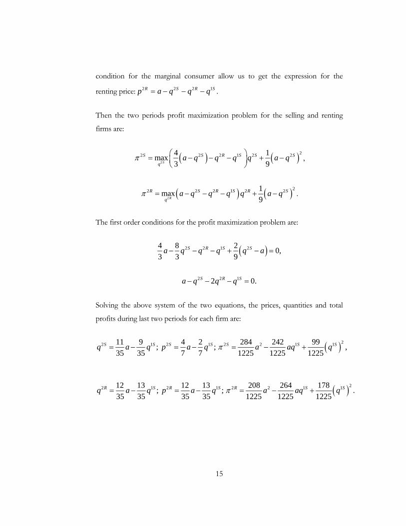
condition for the marginal consumer allow us to get the expression for the

renting price: 2 2 2 1R S R Sp a q q q= − − − .

Then the two periods profit maximization problem for the selling and renting

firms are:

( ) ( )2

22 2 2 1 2 24 1max3 9S

S S R S S S

qa q q q q a qπ ⎛ ⎞= − − − + −⎜ ⎟

⎝ ⎠,

( ) ( )2

22 2 2 1 2 21max9R

R S R S R S

qa q q q q a qπ = − − − + − .

The first order conditions for the profit maximization problem are:

( )2 2 1 24 8 2 0,3 3 9

S R S Sa q q q q a− − − + − =

2 2 12 0.S R Sa q q q− − − =

Solving the above system of the two equations, the prices, quantities and total

profits during last two periods for each firm are:

( )22 1 2 1 2 2 1 111 9 4 2 284 242 99; ; ,35 35 7 7 1225 1225 1225

S S S S S S Sq a q p a q a aq qπ= − = − = − +

( )22 1 2 1 2 2 1 112 13 12 13 208 264 178; ; .35 35 35 35 1225 1225 1225

R S R S R S Sq a q p a q a aq qπ= − = − = − +

16

The second period analysis revised

The total profits that correspond to each of four considered above scenarios in

the second period are represented in the Table 2:

Table 2

Total Profits, Three-Period Model, Second Period

Firm 1 Firm 2

Renting Selling

,RR RRπ π ,RS SRπ π

Renting

Selling ,SR RSπ π ,SS SSπ π

( )21 2

9 9

SRR

a q aπ−

= + - is total profit that corresponds to situation when both

firms rent;

( )22 1 111 11 2764 64 256

SS S Sa aq qπ = − + - is total profit that corresponds to situation

when both firms sell;

( )22 1 1284 242 991225 1225 1225

SR S Sa aq qπ = − + - is total profit of selling firm that

corresponds to situation when one firm sells and another one rents;

( )22 1 1208 264 1781225 1225 1225

RS S Sa aq qπ = − + - is total profit of renting firm that

corresponds to situation when one firm sells and another one rents.

17

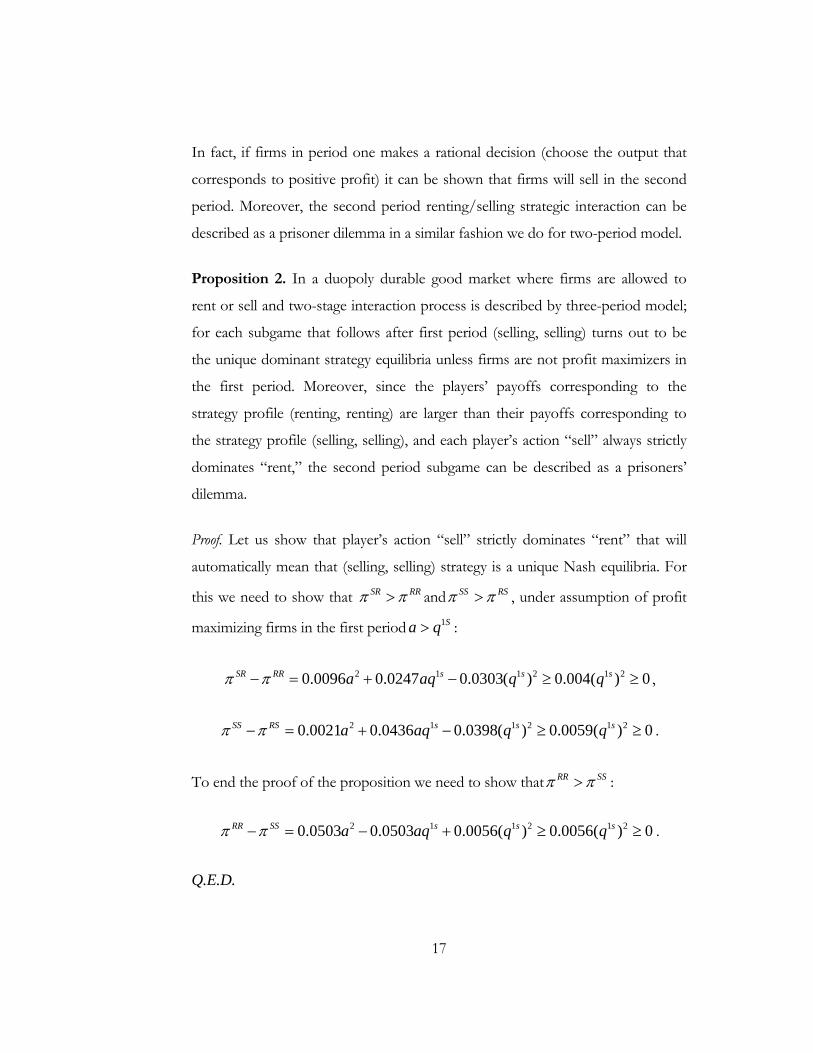
In fact, if firms in period one makes a rational decision (choose the output that

corresponds to positive profit) it can be shown that firms will sell in the second

period. Moreover, the second period renting/selling strategic interaction can be

described as a prisoner dilemma in a similar fashion we do for two-period model.

Proposition 2. In a duopoly durable good market where firms are allowed to

rent or sell and two-stage interaction process is described by three-period model;

for each subgame that follows after first period (selling, selling) turns out to be

the unique dominant strategy equilibria unless firms are not profit maximizers in

the first period. Moreover, since the players’ payoffs corresponding to the

strategy profile (renting, renting) are larger than their payoffs corresponding to

the strategy profile (selling, selling), and each player’s action “sell” always strictly

dominates “rent,” the second period subgame can be described as a prisoners’

dilemma.

Proof. Let us show that player’s action “sell” strictly dominates “rent” that will

automatically mean that (selling, selling) strategy is a unique Nash equilibria. For

this we need to show that SR RRπ π> and SS RSπ π> , under assumption of profit

maximizing firms in the first period 1Sa q> :

2 1 1 2 1 20.0096 0.0247 0.0303( ) 0.004( ) 0SR RR s s sa aq q qπ π− = + − ≥ ≥ ,

2 1 1 2 1 20.0021 0.0436 0.0398( ) 0.0059( ) 0SS RS s s sa aq q qπ π− = + − ≥ ≥ .

To end the proof of the proposition we need to show that RR SSπ π> :

2 1 1 2 1 20.0503 0.0503 0.0056( ) 0.0056( ) 0RR SS s s sa aq q qπ π− = − + ≥ ≥ .

Q.E.D.

18

The first period

There are four subgames that follow after pre-play stage of the game: RR – when

both firms choose to rent in the first period, SR and RS – when one firm chooses

to rent and other to sell in the first period, and SS – when both firms sell in first

period. For case when firms make their renting/selling decisions in each period

only SS second period scenario should be considered. However, we consider all

four second period scenarios that will be used for analyzing the case when firms

make their renting/selling choices on pre-play stage of the game.

The first period, RR subgame

In this case, decisions made in the first period do not affect decisions to be made

in the next two periods. As a result, in the first period Cournot’s equilibria is

achieved with quantities 1

3R

taq = , prices 1

3R

tap = and profit 21

9a . For each

scenario, the total profit is equal to 219

a plus the profit obtained in the first

period plus the profit obtained in the two other periods (derived in previous

section) taking into account that 1 0Sq = . The results are summarized in the

Table 3:

Table 3 Total Profits, Three-Period Model, RR Subgame

Firm 1 Firm2

Renting Selling

2 20.3333 ,0.3333a a 2 20.2809 ,0.3429a a

Renting

Selling 2 20.3429 ,0.2809a a 2 20.2830 ,0.2830a a

19

The first period, SS subgame

As before, the marginal consumer should be studied to identify the inverse

demand curve in the period under consideration. There are different conditions

for the marginal consumer depending on the strategies the firms choose in the

second period. Let us consider all possible cases:

a) Scenario (SR, SR). The marginal consumer is indifferent between buying the

good in the first period and waiting till the second period and then renting the

good. It implies ( ) ( )1 1 1 22 S S S Ra q p a q p− − = − − . Substituting the value of 2Rp

into the last equality the inverse demand curve is: ( )1 143

S Sp a q= − .

b) The scenarios (SS, SR), (SR, SS) and (SS, SS). The marginal consumer is

indifferent between buying the good in the first period and then renting the good

for one period, and waiting till the second period and then buying the good. It

implies ( ) ( ) ( )1 1 1 3 1 22 2S S S R S Sa q p a q p a q p− − + − − = − − . Substituting the

value of 3Rp and 2Sp into the last equality gives the inverse demand curves:

1 111 238 16

S Sp a q= − for the (SS, SS) scenario, and 1 147 4835 35

S Sp a q= − for both

(SS, SR) and (SR, SS) scenarios.

For each of the scenarios, the three-period maximization problem can be written

as:

11

1 1 1 21 1 1max ,

S

S S S j

qp qπ π= +

12

1 1 1 22 2 2max , , .

S

S S S j

qp q j S Rπ π= + =

20

The first-order conditions for the maximization problem for each scenario give

us two equations with two unknowns: 11

Sq and 12

Sq . Solving these two equations

simultaneously, we compute the quantities to be produced by each of the firms in

the first period. The corresponding profits are presented in the table below:

Table 4 Total Profits, Three-Period Model, SS Subgame

Firm 1 Firm2

Renting Selling

2 20.2830 ,0.2830a a 2 20.2557 ,0.2818a a

Renting

Selling 2 20.2818 ,0.2574a a 2 20.2562 ,0.2562a a

SR and RS Subgames

By symmetry, we assume that the first firm sells and the second firm rents (in the

other words, the SR subgame is considered). As in the SS subgame case, different

conditions for the marginal consumer depending on which strategies the firms

choose in the second period are to be specified. Moreover, in order to identify

not only the inverse demand curve for the selling firm, but also the demand faced

by the renting firm, some market clearing conditions should be analyzed. Let us

derive each firm’s inverse demand curve for the possible scenarios that are

present in the SR subgame:

a) The scenario (SR, RR). The marginal consumer is indifferent between buying

the good in the first period and waiting till the second period and then renting the

good. It implies: ( ) ( )1 1 1 1 1 22 S R S S R Ra q q p a q q p− − − = − − − . Substituting the

value of 2Rp into the last equality the inverse demand curve gives

21

us: ( )1 1 143

S S Rp a q q= − − . The marketing clearing condition give as the inverse

demand curve for the renting firm: 1 1 1R S Rp a q q= − − .

b) The scenarios (SS, RR), (SR, RS) and (SS, RS). Marginal consumer is

indifferent between buying the good in the first period and then renting good

during one period, and waiting till the second period and then buying the good. It

implies ( ) ( )1 1 1 1 1 3 1 1 22( ) 2S R S S R R S R Sa q q p a q q p a q q p− − − + − − − = − − − .

Substituting the value of 3Rp and 2Sp into the last equality gives the inverse

demand curves: 1 1 161 4348 32

S S Rp a q q= − − for the (SS, RS) scenario,

and 1 1 147 4835 35

S S Rp a q q= − − for both (SS, RR) and (SR, RS) scenarios.

The marketing clearing condition for each scenario is 1 1 2S R Rp p p= + , which

leads to the same inverse demand curve for the renting firm: 1 1 1R S Rp a q q= − − .

As a result, for each scenario, the three-period maximization problem can be

written as:

1

1 1 1 21max ,

S

S S S j

qp qπ π= +

1

1 1 1 22max , , .

R

R R R j

qp q j S Rπ π= + =

The first-order conditions for the maximization problem for each scenario are

given by two equations that can be easily solved. The corresponding profits are:

22

Table 5

Total Profits, Three-Period Model, SR Subgame

Firm 1 Firm2

Renting Selling

2 20.3429 ,0.2809a a 2 20.2964 ,0.2918a a

Renting

Selling 2 20.3559 ,0.2359a a 2 20.2856 ,0.2509a a

The whole game, firms make their decisions in each period

To summarize first period selling/renting strategic interaction, three-period firms’

payoffs are represented in the table below:

Table 6

Total Profits, Three-Period Model, Whole Game

Firm 1 Firm2

Renting Selling

2 20.2830 ,0.2830a a 2 20.2509 ,0.2856a a

Renting

Selling 2 20.2856 ,0.2509a a 2 20.2562 ,0.2562a a

It is easy to verify that the strategy profile (selling, selling) is the unique Nash

equilibria for the first-period game, taking into account the players’ actions in the

second period. We single out with subgame perfect equilibria that can be formally

stated in a form of proposition:

23

Proposition 3. In a duopoly durable good market where the firms are allowed to

rent or sell, live for three periods, produce three-period durable goods and make

their renting/selling decisions in each period, the strategy profile (selling, selling)

in the first period and (selling, selling) in the second period turns out to be the

unique subgame perfect equilibria.

The whole game, firms make their decisions in the first period

In this case, there are four strategies for each player. For example, the

renting/selling (RS) strategy corresponds to the case when firm rents in the first

period and sells in the second period. Above we considered all possible scenarios

for this game. Let us summarize firms’ profits in the table:

Table 7

Total Profits, Three-Period Model, Pre-Play Stage

Firm1 Firm2

RR RS SR SS

2 20.3333 ,0.3333a a 2 20.2809 ,0.3429a a 2 20.2809 ,0.3429a a 2 20.2359 ,0.3559a a

2 20.3429 ,0.2809a a 2 20.2830 ,0.2830a a 2 20.2918 ,0.2964a a 2 20.2509 ,0.2856a a

2 20.3429 ,0.2809a a 2 20.2964 ,0.2918a a 2 20.2830 ,0.2830a a 2 20.2557 ,0.2818a a

RR

RS

SR

SS 2 20.3559 ,0.2359a a 2 20.2856 ,0.2509a a 2 20.2818 ,0.2557a a 2 20.2562 ,0.2562a a

From Table 7 we can easily find out all Nash equilibria. Our findings can be

formally stated as a proposition:

24

Proposition 4. In a duopoly durable good market where firms are allowed to

rent or sell, live for three periods, produce goods with two-period durability and

make their renting/selling decisions in the first period; strategies profiles (SS, SS),

(SR, RS) and (RS, SR) are Nash equilibria. Moreover, strategy (renting/renting) is

strictly dominated by other three strategies (selling/selling), (selling/renting) and

(renting/selling).

So, we find out strict evidence that firms will commit to selling strategy in the

case when firms make their renting/selling decisions in each period. However,

under another specification, when firms make their renting/selling decisions only

in the first period there are also the possibility of choosing renting strategy in one

period and selling strategy in another one. It is worth to mention that firms more

likely to sustain equilibria (SR, RS) and (RS, SR) than equilibria (SS, SS) because

of two main reasons. First of all, firms get higher profit in equilibria (SR, RS) and

(RS, SR). Second, even if in a process of reaching one of two equilibria (SR, RS)

or (RS, SR) firms misunderstand each other and both choose the same strategy

(renting/selling) or (selling/renting) they pick up with higher profit that under

(SS,SS) equilibria ( 2 20.2830 0.2562a a> ).

4.2 The Case of Three-Period Durability

In this section we discuss the results of three-period model for the case when

durability of good is three periods (perfect durability). Since after first period

firms observe permanent decrease in demand for good by quantity sold in first

period, the subgame that follows after first period is two-period game with

demand function 1SQ a P a q P= − = − −% . As a result, total profits during last two

periods are:

25

Table 8

Total Profits, Three-Period Model, Three-Period Durability, Second Period

.Firm 1 Firm 2

Renting Selling

( ) ( )2 2

1 12 2,9 9

S Sa q a q− − ( ) ( )2 2

1 1208 284,

1225 1225S Sa q a q− −

Renting

Selling ( ) ( )2 2

1 1284 208,

1225 1225S Sa q a q− − ( ) ( )2 2

1 111 11,64 64

S Sa q a q− −

We can make the same conclusions that we do for two-period model. The main

result is that in subgame that follows after first period strategy profile (selling,

selling) is a unique Nash equilibria. The corresponding for this strategy profile

quantities and prices in the second and the third periods are (Poddar 2004):

( ) ( )2 2 1 2 11 2

5 1, ;16 2

S S S S Sq q a q p a q= = − = −

( ) ( )3 3 1 3 11 2

1 1, .8 8

R R S R Sq q a q p a q= = − = −

In this section we restrict our analysis only to the case when firms make their

renting/selling decisions in each period and are not considering case when firm

make their renting/selling decisions on pre-play stage because of its complexity

and our belief that it less likely to give some additional insight into the problems

discussed in this paper.

There are four subgames that follow after pre-play stage (when firms choose their

renting/selling strategies): RR, SR, RS and SS and taking into account that in the

26

second period firms choose to sell four corresponding scenarios are possible: (RS,

RS), (SS, RS), (RS, SS) and (SS, SS).

Scenario (RS, RS)

Scenario (RS, RS) produce the same results in terms of total profit as for the case

when durability is two periods. The reason for this is straightforward. Since in the

first period both firms rent, the second and third periods’ demand functions are

not affected by first period’s decision; but in the second period there is no

difference between selling a good with two or three period durability because

people will live only the remaining two periods. As a result 20.2830 .RR aπ =

Scenario (SS, SS)

The marginal consumer is indifferent between buying the good in the first period,

and waiting till the second period and then buying the good for two periods. It

implies: ( ) ( )1 1 1 23 2S S S Sa q p a q p− − = − − or after substituting in the last

equality the expression for 2Sp we get ( )1 132

S Sp a q= − . The profit

maximization problem that corresponds to this scenario can be written as:

( ) ( )21 1 1 11 2 1 2

3 11max , 1,22 64S

t

SS S S S S St t

qa q q q a q q tπ = − − + − − = .


1S 1S2 1

37 37 85a q q 0,32 32 32

− − =

1S 1S1 2

37 37 85a q q 0.32 32 32

− − =

27

Solving the last system simultaneously, the prices, quantities and total profits for

each firm are:

1 1 1 21 2 0.3033 , 0.5902 , 0.2056S S S SSq q a p a aπ= = = = .

Scenario (SS, RS) and (RS, SS)

The marginal consumer is indifferent between buying the good in the first period,

and waiting till the second period and then buying the good for two periods. This

condition implies: ( ) ( )1 1 1 1 1 23 2S R S S R Sa q q p a q q p− − − = − − − or after

substituting in the last equality the expression for 2Sp we

get ( )1 1 132

S S Rp a q q= − − . Additionally, from market clearing condition

1 2 1S S Rp p p= + we get inverse demand function for renting

firm: 1 1 1R S Rp a q q= − − . The profit maximization problem that corresponds to

this scenario can be written as:

( ) ( )21 1 1 13 11max ,2 64

SR S R S Sa q q q a qπ ⎛ ⎞= − − + −⎜ ⎟⎝ ⎠

( ) ( )21 1 1 111 .64

RS S R R Sa q q q a qπ = − − + −


1S 137 85a q 0,32 32

Rq− − =

1S 1a q 2q 0.R− − =

28

Solving the last system simultaneously, the prices, quantities and total profits for

each firm are:

1 1 2 20.3043 , 0.3478 , 0.2949 , 0.2042 .S S SR RSq a p a a aπ π= = = =

The whole game

Table 9 summarizes three-period game:

Table 9

Total Profits, Three-Period Model, Three-Period Durability, Whole Game

Firm 1 Firm2

Renting Selling

2 20.2830 ,0.2830a a 2 20.2042 ,0.2942a a

Renting

Selling 2 20.2942 ,0.2042a a 2 20.2056 ,0.2056a a

It is easy to verify that the strategy profile (selling, selling) is the unique Nash

equilibria for the first-period game, taking into account the players’ actions in the

second period. The situation is quite familiar for us from two-period model,

player’s action “sell” strictly dominates player action “rent” even so the strategy

profile (renting, renting) produces a higher profit for each of the firms than

(selling, selling). This finding can be formally stated in a form of proposition:


rent or sell, live for three periods, produce two-period goods and make their

renting/selling decisions in each period, the strategy profile (selling, selling) in the

29

first period and (selling, selling) in the second period turns out to be the unique

subgame perfect equilibria.

4.3 The Case of Asymmetric Durability

In this section we consider the game with asymmetric durability of the goods.

One firm produces the good with two-period durability and another one with

three-period durability. Without loss of generality, assume that first firm produces

two-period durable good and second firm – three-period durable good. As in

Section 3.3 we are studying only case when firms make their renting/selling

strategies in each period.

In fact, the asymmetry arises only if two firms sell in the first period. If both firms

rent in the first period the model can be viewed as three-period model with two-

period durability of the good with corresponding firms’

profits 1 1 21 2 0.2830R R aπ π= = . The reason for this is the following. After first

period consumers will consider three and two period durable goods as identical

because these goods can be useful for them only during last two periods of their

life. For the same reason the situation when in the first period the first firm rents

and the second sells can be viewed as a model with three-period durability

( 1 2 1 21 20.2042 , 0.2942R Sa aπ π= = ), and the situation when in the first period

the first firm sells and the second rents can be viewed as a model with two-period

durability ( 1 2 1 21 20.2856 , 0.2509S Sa aπ π= = ).

Let us consider the situation when both firms sell in the first period. In the

second period firms observe temporal decrease in the demand for good by

quantity 11

Sq sold by the first firm in the first period, and the permanent decrease

by quantity 12

Sq sold by the second firm. Since there is no difference in the

second period between two and three period durability of the good, the subgame

30

that follows after the first period can be viewed as a subgame of a model with

two-period durability (with substituting a by 12

Sa q− ) .

It means that Proposition 2 holds and firms sell in the second period. The prices,

quantities and total profits during last two periods for each firm are:

( )22 1 2 1 2 2 1 11 1 1 1

5 9 1 1 11 11 27; ; , 1,2,16 32 2 4 64 64 256

S S S S S S St t tq a q p a q a aq q tπ= − = − = − + =% % % %

where 12

Sa a q= −% .

Clearly, in the first period firms will set-up different prices for their products.

Thus, the marginal consumer is indifferent between buying two-period durable

good in the first period and then renting the good for one period, and waiting till

the second period and then buying the good. This condition implies:

( ) ( )1 1 3 1 213 2S S R S Sa q p p a q p− − + = − − or after substituting in the last

equality the expression for 2Sp and 3Rp we get 11 1 2

11 23 118 16 8

S S Sp a q q= − − .

In the same time, the marginal consumer is indifferent between buying three-

period durable good in the first period and waiting till the second period and then

buying the good. It implies ( ) ( )1 1 1 223 2S S S Sa q p a q p− − = − − or after

substituting in the last equality the expression for 2Sp we

get 12 1 2

3 5 32 4 2

S S Sp a q q= − − .

As a result, the three-period maximization problem can be written as:

1

1 1 1 2max , 1, 2S

t

S S S St t t t

qp q tπ π= + = .

31

First-order conditions for the maximization problem are given by two equations

that can be easily solved. The corresponding total profits for scenario (SS, SS)

are: 1 2 1 21 20.2121 , 0.2549S Sa aπ π= = .

The total profits for all scenarios are represented in Table 10:

Table 10

Total Profits, Three-Period Model, Asymmetric Durability

Firm 1 Firm2

Renting Selling

2 20.2830 ,0.2830a a 2 20.2042 ,0.2942a a

Renting

Selling 2 20.2856 ,0.2509a a 2 20.2121 ,0.2549a a

As in the cases with two and three period durability the strategy profile (selling,

selling) is a unique Nash equilibria. Another finding is that under equilibria firms

with higher durability of a good get higher profit. Intuitively, firm that produces

their goods with three-period durability has a strategic advantage in the first

period by charging the prices on the higher level than prices for two-period

durable goods. Our findings can be formally stated in a form of proposition:

Proposition 6. In a duopoly durable good market with asymmetric durability of a

good, where the firms are allowed to rent or sell, live for three periods, and make

their renting/selling decisions in each period, the strategy profile (selling, selling)

in first period and (selling, selling) in second period turns out to be the unique

subgame perfect equilibria. Moreover, in equilibria firm that produces their goods

with higher durability gets higher profit.

32

4.4 Choice of Durability

Assume that additionally to choosing renting/selling strategies and quantities to

be sold, firms choose the durability of their goods. We assume that each firm has

a possibility to choose between three and two period durability. Firms choose the

durability of their goods before choosing whether to rent or to sell and how

much to produce in each period. However, since in the second and third periods

there is no difference between selling the two and three period durable good,

there is only reason to distinguish between choices of the durability made by

firms in the first period.

As a result, the choice of the durability can be thought of as a pre-play stage.

There are four possible scenarios after pre-play stage: both firms produce two-

period durable good (discussed in Section 3.2), both firms produce three period

durable good (discussed in Section 3.3) or one firm produce two period durable

good while another produces three period durable good (discussed in Section

3.4). In each of this scenario firms prefer selling strategy for renting one in each

of three periods. Table 11 summarizes the results of three-period model with the

choice of durability:

Table 11

Total Profits, Three-Period Model, Choice of Durability

Firm 1 Firm2

Two period Three perid

2 20.2562 ,0.2562a a 2 20.2121 ,0.2549a a

Two period

Three period 2 20.2549 ,0.2121a a 2 20.2042 ,0.2042a a

33

Firm’s action “produce two-period durable good” strictly dominates action

“produce three-period durable good”. We single out with subgame perfect

equilibria that can be formally stated in a form of proposition:


rent or sell, live for three periods, can choose the durability of good and make

their renting/selling decisions in each period, the strategy profile where both

firms choose two-period durability of good and selling strategy in each period is

the unique subgame perfect equilibria.

4.5 Limitations

We show that oligopolists will commit to selling strategy if they can choose their

renting/selling strategies in each period. It coincides with previously received

results for two-period model (Poddar 2004). The same conclusions hold for two

and three period durability cases as well as asymmetric durability case. However

there is an incentive to commit to renting strategy in some periods if firms

choose their renting/selling strategies in the first period only. Another finding is

that in the presence of the choice of durability, firms will prefer to produce their

goods with lower durability. However, there are some limitations of our model.

First, we restrict our analysis to three periods only. The reasonable question

arises. What would happen if we consider strategic behavior of oligopolists when

number of periods is more than three periods? Following the intuition behind our

findings, especially Proposition 2, the permanent or temporary decrease in

demand for goods does not affect strategical firm’s renting/selling behavior. So,

the results of three-period model can be used for analyzing subgame that follows

after first period of four-period model, which in the same way can be used for

analyzing five-period model.

34

Knowing that in the following periods it will be optimal to commit to selling

strategy firms can choose between two options: either sell in current period, or

switch to renting strategy. If firm switches to renting strategy it gives an incentive

for opponent to sell their goods for higher prices than renting one and get extra

profit in current period. Also in real world it may be costly to switch from one

strategy to another one from period to period. In this case pre-play stage plays its

important role and firms may commit to renting strategy in a similar fashion we

showed in Section 3.2.

Second, we restrict our analysis to linear demand functions. We do this for two

main reasons. On the one hand, we use it for comparison purpose with two-

period model. On the other hand, even in the case of a linear demand functions

our calculation is quite complicated and we did not find easy way to make some

generalization for the case of other demand functions.

Third, we assume that there is zero cost of production and there is no asymmetry

in a cost of production among firms. While this assumption is sufficient for our

analysis of strategic firm’s behavior (Poddar, 2004), the assumption of different

cost of production two and three-period durable good may be crucial for the

choice of durability analysis.

Since we show that oligopolists prefer to produce goods with lower durability

they should be interested in finding ways to reduce the durability of their goods

that may be associated with some additional cost. Intuitively, there is some level

of durability after which it is not profitable anymore to reduce the durability of

their goods. It happens due to both, reduction of prices and increasing in cost of

producing less durable goods. If we assume that firms have the same access to

technology that reduces durability of a good, they should both commit to this

optimal level of durability.

35

Finally, the absence of discounting factor restricts our analysis in some sense. We

argue that introducing discount factor is unlikely to change our main results. The

first reason is that consumers similar to firms value tomorrow consumption less

than today one. As a result, following Poddar(2004) the second reason is that

firms get lower profit both under renting and selling strategies, and so it should

not change the strategic renting/selling interaction of the firms. We provide

further discussion of discounting problem in the next chapter.

36

C h a p t e r 5

REPEATED INTERACTION MODEL

In this section we discuss how firms’ strategies are affected when firms will

repeatedly interact infinitely many times. The main assumption to be made is that

firms can restrict the durability of their goods to two periods. It can be made by

several ways: increase quality of new supplied goods, introducing new style or

simply decreasing durability of currently supplied goods. Even so this assumption

can be violated in the real world, there are such things as a habit, technological

process or catastrophe that cause consumers to change durable goods from time

to time. Such dynamic processes when one goods are out of the use and others

become popular in the market can be with some approximation described by

repeated interaction model presented below.

Assume that the durability of the good is limited to two or three periods

depending on type of model we are considering. Moreover, we assume that once

firm introduces “new” good nobody will buy “old” goods, even so they may be

still in the market. As a result, discussed above two-period and three-period

models, both with two and three period durability of a good, can be viewed as

infinitely interacted model with payoff matrix representing in Table 1, Table 6

and table 9 correspondingly. We assume that each consumer lives for three or

two periods depending on model that is basis of our analysis. Therefore, there is

no need to introduce discounting factor for consumers. Moreover, this

assumption makes our model even more realistic because new generation of

people is more likely to prefer new sort of goods, while old people may be

opposed to any changes.

37

In infinitely interaction game, based on three-period model with two-period

durability, there are two types of durability: durability because the good is out of

the use (two periods) and durability due to introduction new type of good (three

periods). Such situation we can observe in the computer or mobile phone

markets. Mobile phone can be out of use due to damage of battery, screen or

keyboard. In most cases, such damage can be fixed. However, once new type of

mobile phone is introduced there is no need to supply spares for old models and

such repair is impossible or too expensive in comparison with the price of a new

model of the phone.

As previously, we assume that there is no discounting between two consequent

periods in which one type of goods is in use. However, there is a discounting

factor δ between period when “old” good was in use and period when “new”

good is introduced. This assumption does not confine the analysis presented

below because of two reasons. First of all, firms should be more patient between

two consequent periods when one type of good is in the use because there is

more or less stable demand of their goods in each period. However, once “new”

good is introduced firms are highly interested in compensating their cost for

developing new type of good as soon as possible. Second, even so there is a need

to introduce this discounting between periods, the consumer discounting also

should be introduced and this factors are very likely to compensate each other.

Finally, we are more interested in comparison analysis of how patient firms

should be under different assumptions and specification of the model rather than

in particular values of discount factors.

There are two possible situations that will be considered. The first situation is

when firms sustain renting strategy in each period. The second situation is when

additionally to the sustaining renting strategy they produce half of the monopoly

optimal output in each period. For each of these two cases critical value δ will be

38

found that describes how patient firms should be so that trigger strategy profile

remains credible.

For simplicity of representation of our results we will call each of two (three)

periods during which one type of good is in use as a “sub-period” and two (three)

periods together as a “period”.

Trigger strategies when both firms follow renting strategies in each period

Consider trigger strategy in which each firm cooperates in period t playing renting

strategy as long as other firm cooperates in all previous periods and rents their

goods. However, if opponent did not cooperate and switch to selling strategy in

some sub-period of period t-1, firm will choose selling strategy forever, including

all remaining sub-periods of period t-1. Note, that there is no possibility to

deviate in last sub-period of particular period because there is no difference

between renting and selling. The results for each of three models (two-period

model, three-period model with two-period durability and three-period model

with three-period durability) are stated as the propositions.

Proposition 8.a In a duopoly durable good market where firms are allowed to

rent or sell, consumers live for two periods and durability of the good is two

periods, if the discounting factor 0.16δ ≥ , then the outcome where the players

play their trigger strategies is a subgame perfect equilibria.

Proof. Consider particular period of time t1. Let us calculate the present value of

infinite stream of payoffs if both firms play accordingly to the trigger

strategies: 1 21

0

1 21 9

i RR

iaδ π

δ

∞

=

= ⋅−∑ . If firm deviates in current period by playing

selling strategy then firm gets 1 21

2841225

SR aπ = in current period, but since after

this period other firm will play selling strategy forever in the next period firm will

39

get lower profit 1 21

1164

SS aπ = . As a result, present value that corresponds to

deviation case is 1 1 2 21 1

1

284 11 1 111225 64 1 64

RS i SS

ia aπ δ π

δ

∞

=

⎛ ⎞+ = − + ⋅⎜ ⎟ −⎝ ⎠∑ . From

condition that present value will be higher when firm does not deviate than when

it deviates we find that 0.16δ ≥ . Q.E.D.

Proposition 8.b In a duopoly durable good market where firms are allowed to

rent or sell, consumers live for three periods and durability of the good is two



Proof. The present value of infinite stream of payoffs if both firms play

accordingly to the trigger strategies: 1 21

0

1 11 3

i RR

i

aδ πδ

∞

=

= ⋅−∑ . If firm deviates in

the first sub-period by playing selling strategy then firm gets 1 2 2 1

1 10.2856 0.3333SR RRa aπ π= < = in current period, so it is clearly no sense to

deviate in the first sub-period. If firm deviates in the second sub-period, there is

no difference after first period with two-period model, and as a result it gets

“cooperative” profit 213

a in the first sub-period and 2 21

2841225

SR aπ = in the

second sub-period or totally 20.3429dev aπ = . After this period both firms will

play selling strategies forever and will get lower profit 1 20.2562SS aπ = . Present

value that corresponds to deviation case is

( )1 2 21

1

10.3429 0.2562 0.25621

dev i SS

ia aπ δ π

δ

∞

=

+ = − + ⋅−∑ . From condition that

present value will be higher when firm does not deviate than when it deviates we

find that 0.11δ ≥ . Q.E.D.

40

The only difference between three-period model with three-period durability and

three-period model with two-period durability is that after deviations firms will

get lower profit, specifically 11 0.2056SSπ = . So, we can state the next proposition

without proof:

Proposition 8.c In a duopoly durable good market where firms are allowed to

rent or sell, consumers live for three periods and durability of the good is three



Trigger strategies when both firms produce half of monopoly output in each period

Consider trigger strategy in which each firm cooperates in period t playing renting

strategy and renting half of monopolistic output in each sub-period of period t,

specifically 12 4

Mq a= , and get half of monopolistic profit 212 8

M

aπ= , as long as

other firm cooperates in sub-period t-1. However, if opponent does not

cooperate and switch to the selling strategy on the first stage in some sub-period

of period t-1, or deviates on the second stage and produces * 38

q a= amount of

good with corresponding profit * 2 29 164 8

a aπ = > , firm will choose selling

strategy with Cournot’s quantities forever.

Proposition 9.a In a duopoly durable good market where firms are allowed to

rent or sell, consumers live for three periods and durability of the good is two



41


accordingly to the trigger strategies: 2

0

1 122 1 4

Mi

iaπδ

δ

∞

=

= ⋅−∑ . If firm deviates in

current period by playing selling strategy then firm gets 1 21

2841225

SR aπ = in

current period. If firm deviates on the second stage in the second sub-period of

current period it gets totally * 2 217 2842 64 1225

Mdev a aππ π= + = > . There is no need

to consider deviation on the second stage in the first sub-period because it causes

to *π profit in the first sub-period, but lower than 2

Mπ “punishment” profit in

the second sub-period. After this period both firms will play selling strategies

forever and will get lower profit 1 21164

SS aπ = . Present value that corresponds to

deviation case is 1 2 2

1

17 11 1 11( )64 64 1 64

dev i SS

ia aπ δ π

δ

∞

=

+ = − + ⋅−∑ . From condition

that present value will be higher when firm does not deviate than when it deviates

we find that 0.17δ ≥ . Q.E.D.

Proposition 9.b

In a duopoly durable good market where firms are allowed to rent or sell,

consumers live for three periods and durability of the good is two periods, if the

discounting factor 0.11δ ≥ , then the outcome where the players play their trigger

strategies is a subgame perfect equilibria.


accordingly to the trigger strategies: 2

0

1 322 1 8

Mi

iaπδ

δ

∞

=

= ⋅−∑ . Accordingly to

proof of Proposition 8.b, if firm deviates to selling strategy it gets

42

1 20.3429dev aπ = , but if firms deviates on the second stage in third sub-period

(similarly to proof of Proposition 8.b there is no need to consider deviations in

the second and first sub-periods) it gets higher profit 2 20.3906dev dev aπ π= = .

After this period both firms will play selling strategies forever and will get lower

profit 20.2562SS aπ = . Present value that corresponds to deviation case

is ( )1 2 2

1

10.3906 0.2562 0.25621

dev i SS

ia aπ δ π

δ

∞

=

+ = − + ⋅−∑ . From condition

that present value will be higher when firm does not deviate than when it deviates

we find that 0.12δ ≥ . Q.E.D.

Proposition 9.c is stated without proof because it can be proven by analogy with

Proposition 9.b.

Proposition 9.c In a duopoly durable good market where firms are allowed to

rent or sell, consumers live for three periods and durability of the good is three



Analysis of the results

First of all, according to repeated interaction model, the firms should be not so

patient to sustain trigger strategies. In all six cases, that are considered,

cooperation will be sustainable for 0.17δ ≥ . However, we should take into

account, that we are requiring from firms to be absolutely patient ( 1δ = ) during

two consequent sub-periods within one period. It means that for correct

interpretation, threshold δ -values should be normalized. Thus, got in

Proposition 8.a threshold value is equal to1 0.17 0.592

+= , while according to the

43

Proposition 8.b for three-period model with two-period durability threshold value

equals1 1 0.11 0.693

+ += .

Second, from Proposition 8.b and Proposition 8.c (as well as Proposition 9.b and

Proposition 9.c) we can make a conclusion that firms should be more patient to

sustain trigger strategies with shorter durability of their goods. The intuition

behind this result is the following. As long as firms cooperate there is no

difference between three and two-period durability of the good because renting

strategy allows for firm to maintain prices on the same level during three sub-

periods. However, when firms do not cooperate, longer durability of the good is

associated with lower total profit, and as a result, with higher “punishment” for

deviation.

Finally, we find out that firms that cooperate in renting/selling strategies should

be less patient than firms that cooperate both in renting/selling strategies and in

quantities of good to be produced. The explanation that firms, that cooperate

both in renting/selling strategies and in quantities of good to be produced, have

more possibilities to deviate (additionally in quantities) is not fully correct.

Additional cooperation in quantities is not only associated with higher profit

under deviation, but also with higher punishment due to absence of half of

monopolistic profit in all subsequent periods after deviation. Our finding

indicates that deviation in quantities to be produced is much more profitable than

deviation in selling/renting strategies and, as a result, requires firms to be more

patient in order to sustain trigger strategies.

44

C h a p t e r 6

CONCLUSIONS

In this paper we investigate a three-period simultaneous-move model for

oligopoly market. We show that in the perfect durability case, the firms will

commit to the selling strategy that supports previous findings for two-period

models. Moreover, we extend our analysis to goods with a durability of two

periods, asymmetric durability cases, and prove that our results are robust with

respect to such changes.

We provide the reasons why firms may commit to the renting strategy. The one

reason is the existence of a time lag between announcing a strategy and its

implementation. We determine Nash equilibria for the case when the firms make

their renting/selling decisions each period. Two Nash equilibria are a mixture of

renting/selling strategies, with firms preferring the renting strategy in some

periods and the selling strategy in the others.

The intuition behind our finding is the following. Selling is also a better choice

for oligopoly firms as long as they make their renting/selling decisions each

period. However, if the firms make their second period choices in the first period

the story is different. There is no sense anymore in switching to the selling

strategy each period if the opponent chooses to rent in the first period and sell in

the second period. Instead, the firm sells in the first period, rents in the second to

support a higher demand in the third period.

The second reason is the repeated nature of the firms’ interaction. Under

different assumptions and specifications, we consider trigger strategy equilibria.

We show that it is easier to sustain the renting strategy when the good is more

durable. At the same time, if, additionally to cooperation in choosing the renting

45

strategy, the firms cooperate in quantities they should be more patient to be able

to sustain trigger strategies.

However, the nature of this sustainability is different. Difficulties with

sustainability for the case of short durability of a good are explained by lower

punishment for deviation from renting strategy comparing with long durability

case, while cooperation in quantities is less sustainable due to greater incentive to

deviate from renting strategy.

A possible direction for further research can be found in the jeans market: It

would be interesting to compare the results for monopoly and oligopoly market

structures under the assumption that the cost of production increases when the

good becomes less durable.

46

WORKS CITED

Basu, Kaushik. 1987. Why Monopolists Prefer to Make their Goods Less

Durable. Economica 55: 541-546.

Bulow, Jeremy. 1982. Durable Goods Monopolists. Journal of Political Economy

90: 314-332.

Bulow, Jeremy. 1986. An Economic Theory of Planned Obsolescence. Quartely

Journal of Economics 101: 729-749.

Coase, R.onald. 1972. Durability and Monopoly. Journal of Law and Economics 15:

143-149.

Garella, Paolo. 1999. Rationing in a Durable Goods Monopoly. The RAND

Journal of Economics 30: 44-55.

Garella, Paolo. 2002. Price Discrimination and the Location Choice of a Durable

Goods Monopoly. Regional Science and Urban Economics 32: 765-773.

Goering, Gregory. 1993. Durability Choice Under Demand Uncertainty.

Economica 60: 397-411.

Goering, Gregory. 2005. Durable Goods Monopoly and Quality Choice. Research

in Economics 59: 59-66.

Goering, Gregory. 2008. Socially Concerned Firms and the Provision of Durable

Goods. Economic Modelling 25: 575-583.

Inderst, Roman. 2008. Durable Goods with Quality Differentiation. Economics

Letters 100: 173-177.

47

Kumar, Praveen. 2002. Price and Quality Discrimination in Durable Doods

Monopoly with Resale Trading. International Journal of Industrial Organization 20:

1313-1339.

Mann, Duncan. 1992. Durable Goods Monopoly and Maintenance. International

Journal of Industrial Organization 10: 65-79.

Malueg, David, John Solow. 1987. On Requiring the Durable Goods Monopolist

to sell. Economics Letters 25: 283-288.

Poddar, Sougata. 2004. Strategic Choice in Durable Goods Market when Firms

Move Simultaneously. Research in Economics 58: 175-186.

Suslow, Valerie. 1986. Commitment and Monopoly Pricing in Duable Goods

Models. International Journal of Industrial Organization 4: 451-460.

Sagasta, Amagoia, Ana Saracho. 2008. Mergers in Durable Goods Industries.

Journal of Economic Behavior & Organization 68: 691-701.

Saggi, Kamal, Nikolaos Vettas. 2000. Leasing Versus Selling and Firm Efficiency

in Oligopoly. Economics Letters 66: 361-368.

Optimal renting /selling strategies in oligopoly durable goods markets

Documents

Transcript of Optimal renting /selling strategies in oligopoly durable goods markets