Optimal Real-Time Sampling Rate Assignment for Wireless ...

Optimal Real-Time Sampling RateAssignment for Wireless Sensor Networks

XUE LIU, QIXIN WANG, WENBO HE, MARCO CACCAMO, and LUI SHA

University of Illinois at Urbana-Champaign

How to allocate computing and communication resources in a way that maximizes the effectiveness

of control and signal processing, has been an important area of research. The characteristic of a

multi-hop Real-Time Wireless Sensor Network raises new challenges. First, the constraints are

more complicated and a new solution method is needed. Second, a distributed solution is needed to

achieve scalability. This article presents solutions to both of the new challenges. The first solution

to the optimal rate allocation is a centralized solution that can handle the more general form

of constraints as compared with prior research. The second solution is a distributed version for

large sensor networks using a pricing scheme. It is capable of incremental adjustment when utility

functions change. This article also presents a new sensor device/network backbone architecture—

Real-time Independent CHannels (RICH), which can easily realize multi-hop real-time wireless

sensor networking.

Categories and Subject Descriptors: C.2.2 [Computer-Communication Networks]: Network

Protocols—Applications; C.3 [Special-Purpose and Application-Based Systems]—Real-timeand embedded systems

General Terms: Algorithms, Design, Performance, Experimentation

Additional Key Words and Phrases: Sensor network, real-time wireless sensor network, optimiza-

tion, pricing, distributed algorithms

1. INTRODUCTION AND RELATED WORK

Real-Time Wireless Sensor Network (RTWSN) is expected to carry out variousapplications such as remote control or video/audio monitoring in ad hoc envi-ronments. Instead of using conservative (lowest allowed) sampling/actuatingrates (since sampling and actuating rate allocation are similar, unless explic-itly denoted, “sampling rate” is used instead of “sampling/actuating rate” in

This research is supported by (listed in alphabetical order) MURI N00014-01-0576, NSF ANI 02-

21357, NSF CCR 02-09202, and ONR N00014-02-1-0102. The first two authors are also supported

by Saburo Muroga Fellowship and Vodaphone Fellowship, respectively.

Part of this research has been published at the 24th IEEE Real-Time Systems Symposium [Liu

et al. 2003].

Authors’ address: Department of Computer Science, University of Illinois at Urbana-Champaign,

Urbana, IL 61801; email: {xueliu,qwang4,wenbohe,mcaccamo,lrs}@cs.uiuc.edu.

Permission to make digital or hard copies of part or all of this work for personal or classroom use is

granted without fee provided that copies are not made or distributed for profit or direct commercial

advantage and that copies show this notice on the first page or initial screen of a display along

with the full citation. Copyrights for components of this work owned by others than ACM must be

honored. Abstracting with credit is permitted. To copy otherwise, to republish, to post on servers,

to redistribute to lists, or to use any component of this work in other works requires prior specific

permission and/or a fee. Permissions may be requested from Publications Dept., ACM, Inc., 1515

Broadway, New York, NY 10036 USA, fax: +1 (212) 869-0481, or [email protected]© 2006 ACM 1550-4859/06/0500-0263 $5.00

ACM Transactions on Sensor Networks, Vol. 2, No. 2, May 2006, Pages 263–295.

264 • X. Liu et al.

the following), a sampling rate allocation that maximizes global utility whilemaintaining real-time schedulability is wanted.

Resource allocation has been studied in general for computing systems[Kurose and Simha 1989; Waldspurger and Weihl 1994; Bolot et al. 1994]. Re-cently, the problem of resource allocation and congestion control in network hasbeen studied together by Kelly and others [Kelly et al. 1998; Kelly 1997; Lowand Lapsley 1999]. However, these works do not consider real-time constraints,and therefore cannot be directly applied to real-time systems.

Stoica et al. [1996] have studied a proportional share resource allocationalgorithm for real-time, time-shared systems. The scheme is for single proces-sor scheduling and is more focused on fairness of the scheduling algorithmsrather than system optimality. Finding the optimal control rates subject toschedulability constraints was first studied by Seto et al. [1996] and by Shaet al. [2000] for analog and digital controllers respectively. An offline solutionmethod is given based on the Kuhn-Tucker condition. However, the schedula-bility analysis is still for a single processor. Rajkumar et al. [1997] investigatedthe QoS-based Resource Allocation Model (Q-RAM), which is capable of han-dling complex multiple quality dimensions. But the solution can only be usedwith single constraint scenario. In the following works, Lee et al. [1999] andGhosh et al. [2003] studied the scenario under multiple constraints. However,the problem they studied is an integer programming problem, which is dif-ferent from the model we will discuss in this article. In Lee et al. [1999], theinteger programming problem is proven to be NP-Hard. Several suboptimal al-gorithms are proposed. According to Ghosh et al. [2003], the one that scales wellis Hierarchical Q-RAM. However, that algorithm requires the division of mul-tiple constraints into independent groups, which is impractical for multi-hopRTWSN.

RTWSN presents new challenges for real-time resource allocation. Routesin a RTWSN may interleave with each other. The sampling rate optimizationmust take into consideration the traffic contention at each router. This makesthe optimization problem harder than those studied before. We present anInterior Point Method (IPM)-based solution to show how the optimal rates canbe found efficiently. On the other hand, though a centralized method is usuallyefficient for small and moderately large RTWSNs, it may not scale well for verylarge RTWSNs, because control messages for optimization converge at the cen-tral node and create a bottleneck. To dynamically find the global optimum in avery large network, a distributed solution is needed to generate balanced opti-mization control traffic that avoids bottlenecks. In addition, the solution shouldbe incremental, so that when the utility functions at a few nodes change, anupdated optimum can be found with small cost.

To the best of our knowledge, the work by Caccamo et al. [2002] is the firstto provide real-time support for multi-hop RTWSN. In Caccamo et al. [2002], acellular base station layout is deployed as the backbone for the whole RTWSN,as shown in Figure 1. The base station network uses seven nonoverlappingRadio Frequency (RF) bands. At the center of each cell, there is one base sta-tion, which also functions as a router. A router in a cell labeled i has a singletransmitter that always transmits at RF band i, and a single receiver that

ACM Transactions on Sensor Networks, Vol. 2, No. 2, May 2006.

Optimal Real-Time Sampling Rate Assignment • 265

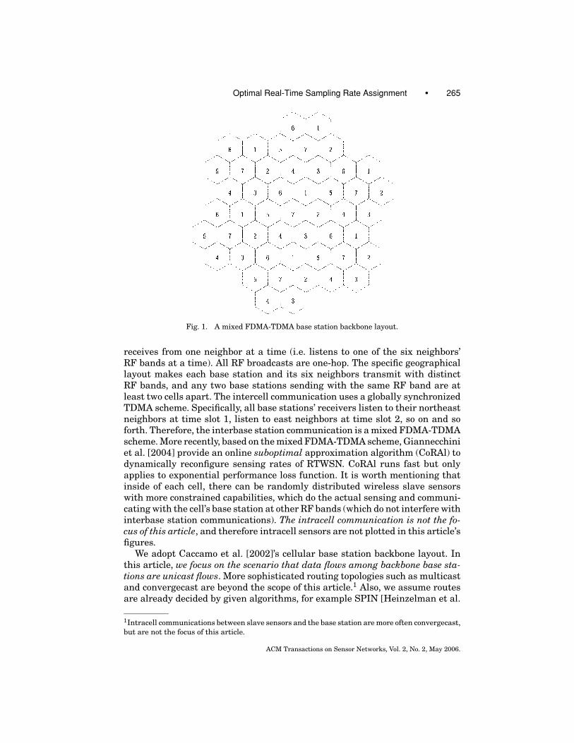
Fig. 1. A mixed FDMA-TDMA base station backbone layout.

receives from one neighbor at a time (i.e. listens to one of the six neighbors’RF bands at a time). All RF broadcasts are one-hop. The specific geographicallayout makes each base station and its six neighbors transmit with distinctRF bands, and any two base stations sending with the same RF band are atleast two cells apart. The intercell communication uses a globally synchronizedTDMA scheme. Specifically, all base stations’ receivers listen to their northeastneighbors at time slot 1, listen to east neighbors at time slot 2, so on and soforth. Therefore, the interbase station communication is a mixed FDMA-TDMAscheme. More recently, based on the mixed FDMA-TDMA scheme, Giannecchiniet al. [2004] provide an online suboptimal approximation algorithm (CoRAl) todynamically reconfigure sensing rates of RTWSN. CoRAl runs fast but onlyapplies to exponential performance loss function. It is worth mentioning thatinside of each cell, there can be randomly distributed wireless slave sensorswith more constrained capabilities, which do the actual sensing and communi-cating with the cell’s base station at other RF bands (which do not interfere withinterbase station communications). The intracell communication is not the fo-cus of this article, and therefore intracell sensors are not plotted in this article’sfigures.

We adopt Caccamo et al. [2002]’s cellular base station backbone layout. Inthis article, we focus on the scenario that data flows among backbone base sta-tions are unicast flows. More sophisticated routing topologies such as multicastand convergecast are beyond the scope of this article.1 Also, we assume routesare already decided by given algorithms, for example SPIN [Heinzelman et al.

1Intracell communications between slave sensors and the base station are more often convergecast,

but are not the focus of this article.



1999], GPSR [Karp and Kung 2000], GEAR [Xu et al. 2001], SPEED [He et al.2003] or Rumor Routing [Braginsky and Estrin 2002] and soforth2; and the to-tal data bandwidth of each one-hop wireless link is adjusted so that the wirelessmedium is reliable enough for real-time communication. (According to informa-tion theory and CDMA theory [Viterbi 1995] (also see Appendix A), if the worstcase wireless medium condition is given, there is an upper bound on data bitthroughput so that the data bit error rate can be maintained below an upperbound.) How to incorporate routing and tolerate device failures and messagedrops into our sampling rate optimization, are future research issues beyondthe scope of this article. According to information theory, the interbase stationbandwidth available is determined by wireless medium quality and receptionquality requirements, and is fundamentally irrelevant with specific multipleaccess schemes, such as FDMA, TDMA or CDMA. The mixed FDMA-TDMAmultiple access scheme proposed in Caccamo et al. [2002] provides poorer flex-ibility on bandwidth allocation adjustment, and the scheduling mechanism ismore complicated. Therefore, in this article, we propose a mixed FDMA andDirect Sequence Spread Spectrum CDMA (DSSS-CDMA)3 scheme called Real-time Independent CHannels (RICH), which provides better flexibility and whosereal-time scheduling is easier to implement and analyze. A brief tutorial onDSSS-CDMA is provided in Appendix A.

The major contributions of this article are:

—Study and model the optimal rate assignment problem in RICH multi-hopRTWSN using real-time schedulability analysis and nonlinear optimization.

—Using the state-of-the-art methods in optimization, two solutions to the opti-mal rate assignment problem are given. One is in a centralized fashion usingthe Interior Point Method, the other is in a distributed fashion based on apricing scheme.

—Compare the trade-offs between the centralized and distributed algorithmsunder different situations.

The rest of the article is organized as follows. Section 2 describes our proposedRICH architecture, which can easily support multi-hop real-time networking.We also give the real-time schedulability constraints analysis in this section.An example of RICH RTWSN is presented to show the practicability of RICH.In Section 3, we formulate the optimal QoS sampling rate assignment probleminto a nonlinear programming problem. Sections 4 and 5 give centralized anddistributed solution for optimal QoS sampling rate assignment respectively. InSection 6, we first compare the numerical solutions based on the example dis-cussed in Section 2, discuss in details the trade-offs between the centralized anddistributed solution. Then we analyze the possible problems and solutions as-sociated with both methods. Finally, conclusions and future work are discussedin Section 7.

2A good survey of routing protocols in sensor networks is given in Akkaya and Younis [2005].3Nowadays, the term CDMA usually refers to DSSS-CDMA.



Fig. 2. Internal architecture of a RICH base station.

2. SUPPORTING MULTI-HOP RTWSN

2.1 RICH Architecture

We assume our wireless base stations (the so-called RICH base stations) havethe internal architecture illustrated by Figure 2. Each RICH base station hasseven DSSS-CDMA modulation/demodulation co-processors (CoPUs), each op-erates with a distinct DSSS-CDMA Pseudo Noise (PN) sequence at a distinctFDMA RF band. Among which, six of the DSSS-CDMA CoPUs are receivers,and the other one is the only transmitter at the base station. We allow the databit bandwidths of each DSSS-CDMA CoPU to be distinct. For the time being,suppose the singular transmitter sends packets according to Earliest DeadlineFirst (EDF) scheduling algorithm. A dedicated EDF scheduling queue is at-tached to it to buffer/schedule the outgoing packets. In addition, a RICH basestation also includes a sensing CoPU, or an intracell communication CoPU thatgathers data from intracell slave sensors. The CPU interacts with each CoPUby periodical polling.

We adopt the cellular base station layout of Caccamo et al. [2002] (seeFigure 3), and maintain the seven RF band coloring of the cells. Meanwhile,we deploy forty-nine DSSS-CDMA PN sequences, denoted as A1, . . . , A7,B1, . . . , B7, C1, . . . , C7, D1 . . . , D7, E1, . . . , E7, F1, . . . , F7, G1, . . . , and G7respectively. In a cell labeled X Y , the RICH base station transmitter deploys



Fig. 3. The mixed FDMA-CDMA base station backbone layout.

the X Y th PN sequence for DSSS-CDMA modulation, and transmits at the Y thRF band. For example, the base station in a cell labeled G7 transmits with theG7th DSSS-CDMA PN sequence at the 7th RF band. The transmission range ofevery transmitter in our RICH RTWSN is one-hop. Each of the six receivers ona RICH base station listens to one of its one-hop neighbor’s transmissions. Takethe RICH base station at a cell labeled A5 for example, its six receivers listento the 6, 7, 4, 1, 3, 2th RF band respectively, and demodulate with DSSS-CDMAPN sequence A6, A7, A4, G1, F3, F2 respectively.

Under such a design, the broadcast of a base station is simultaneously re-ceived by its six one-hop neighbors. The effective receiver is designated by thebroadcast packet’s “destination” data segment. More importantly, because ofthe deployment of DSSS-CDMA, any transmission can be carried out indepen-dently. For example, in Figure 3, an F2 base station and an A6 base stationcan both send packets to an A5 base station (their common one-hop neighbor)at any time. Furthermore, the schedule can be independently adjusted to bespecific per base station. For example, the F2 base station can dedicate 100%of its time sending to the A5 base station; at the same time, the A6 base stationcan dedicate 1

3of its time to the A5 base station. There are no synchronization

requirements between any pair of transmissions. Under TDMA, however, thisis impossible. For example, F2’s sending schedule must not overlap with A6’s.Such mutually exclusive relationships propagate throughout the network; fi-nally all base stations’ broadcast schedules are interlocked, which complicatesanalysis and reconfiguration.



Also, the layout guarantees two base stations transmiting with same DSSS-CDMA PN sequence (and therefore at the same RF band) are at least eighthops away. This implies that a base station does not have to be at the center ofits cell.

2.2 Schedulability Analysis of RICH RTWSN

The broadcast of a RICH base station is overheard by all of its six neighbor basestations. Usually, the wireless medium conditions to the six neighbors are ir-regular [Zhou et al. 2004; Zhao and Govindan 2003]. According to DSSS-CDMAtheory (see Appendix A), given RF band, worst case wireless medium conditions,and maximum acceptable bit error rate, the upper bound of data bit bandwidthis determined—which we call affordable bandwidth. Suppose for a RICH basestation X , because of the irregularity of the wireless medium, the affordablebandwidths to its six neighboring RICH base stations are B1, B2, . . . , B6. Weset the transmission data bit bandwidth of X to be B = min{B1, B2, . . . , B6}.Therefore the broadcast of X is reliably received by all of its six neighbors—thebit error rate of one-hop transmission is always below the maximum accept-able bound. In another words, B models factors such as the impact of radioirregularity on the wireless medium.

For a RICH base station, the real-time scheduling is carried out in theEDF scheduling queue attached to its singular transmitter. Let T be the setof all routes that go through it. For a route τ ∈ T , suppose it has a sam-pling/reporting rate of fτ , and each report is a packet of length lτ . The corre-sponding transmission time of the packet is therefore cτ = lτ /B. When thereare multiple contending routes through one RICH base station, the transmit-ter should be regarded as a nonpreemptive resource, because once a packetstarts transmitting, it cannot be preempted until it is completely transmit-ted. Therefore, the real-time scheduler of a RICH base station’s EDF queueshould be a nonpreemptive EDF scheduler to ensure both the EDF behavior andnonpreemptive usage of the broadcast link. Under such scheduling, a packet(job) can be blocked by at the most, one other packet. Therefore we can applythe well-known schedulability bound for the nonpreemptive EDF scheduler asfollows [Buttazzo 1997]:

∑τ∈T

cτ fτ + Cj f j ≤ 1, for each j ∈ T , (1)

where Cj is the maximum blocking time for sending a packet of route j .

Cj = max{τ∈T and τ �= j }

{cτ }

= max{τ∈T and τ �= j }

{lτ

B

}

= max{τ∈T and τ �= j }

{lτ }B

.



Therefore (1) is transformed into:∑τ∈T

lτ

Bfτ + L j

Bf j ≤ 1, for each j ∈ T , (2)

where L j = max{τ∈T and τ �= j }{lτ }.Multiply both sides of Equation (2) with broadcast link bandwidth B; we get:∑

τ∈Tlτ fτ + L j f j ≤ B, for each j ∈ T . (3)

Besides being a router, a RICH base station can also simultaneously functionas the source end of a route. The data are either from the base station’s localsensing CoPU or by gathering intracell slave sensors’ readings. Either way, thebase station can be regarded as the virtual singular source end sensor for theroute, and its sampling rate is upper bounded, creating the following constraint(for the time being, we assume each base station can be the source end of at themost one route):

f j ≤ f maxj , (4)

where f j is the sampling rate of route j , and f maxj is the maximum afford-

able sampling rate at the route’s source end base station.4 By analyzing eachbase station of the RICH RTWSN according to inequality set (3) and each routeaccording to inequality (4), we can derive a set of linear inequalities, which arethe sufficient real-time schedulability constraints for RICH RTWSN samplingrate assignment. We can summarize them in the following form:{

A f ≤ W

f ≤ f max,(5)

where f = ( f1, f2, . . . , f N )T is the vector of sampling rates assigned to each ofthe N routes. f max = ( f max

1 , f max2 , . . . , f max

N )T is the maximum sampling ratefor the N end point sensors (see (4)). Matrix A and vector W are obtained bybase station-wise analysis according to (3), which reflects the specific routingtopology of the RICH RTWSN. Suppose this schedulability analysis generatesM inequalities in total, then A ∈ R

M×N , W ∈ RM×1.

Besides the constraints from real-time schedulability, there are often appli-cation specific minimum sampling/reporting rate requirements. These extrarequirements can be written as:

f ≥ f min = (f min

1 , . . . , f minN

)T. (6)

Inequality sets (5) and (6) constitute a complete set of real-time schedulabil-ity constraints for RICH RTWSN sampling rate allocation. An example is givenas follows:

4In this article, we assume the capacity of CPU, internal bus, sensing CoPU and RF CoPUs are big

enough, so that as long as (4) is satisfied, we only need to be concerned about the wireless network

bandwidth schedulability.



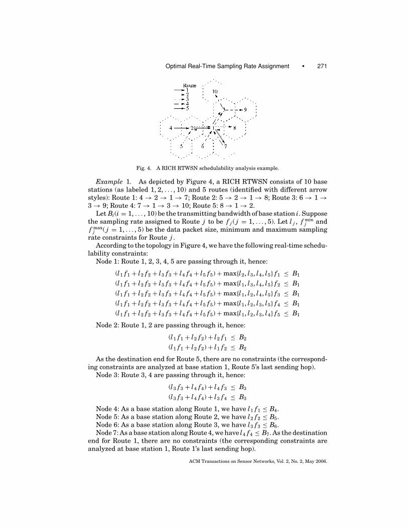
Fig. 4. A RICH RTWSN schedulability analysis example.

Example 1. As depicted by Figure 4, a RICH RTWSN consists of 10 basestations (as labeled 1, 2, . . . , 10) and 5 routes (identified with different arrowstyles): Route 1: 4 → 2 → 1 → 7; Route 2: 5 → 2 → 1 → 8; Route 3: 6 → 1 →3 → 9; Route 4: 7 → 1 → 3 → 10; Route 5: 8 → 1 → 2.

Let Bi(i = 1, . . . , 10) be the transmitting bandwidth of base station i. Supposethe sampling rate assigned to Route j to be f j ( j = 1, . . . , 5). Let l j , f min

j andf max

j ( j = 1, . . . , 5) be the data packet size, minimum and maximum samplingrate constraints for Route j .

According to the topology in Figure 4, we have the following real-time schedu-lability constraints:

Node 1: Route 1, 2, 3, 4, 5 are passing through it, hence:

(l1 f1 + l2 f2 + l3 f3 + l4 f4 + l5 f5) + max{l2, l3, l4, l5} f1 ≤ B1





Node 2: Route 1, 2 are passing through it, hence:

(l1 f1 + l2 f2) + l2 f1 ≤ B2

(l1 f1 + l2 f2) + l1 f2 ≤ B2

As the destination end for Route 5, there are no constraints (the correspond-ing constraints are analyzed at base station 1, Route 5’s last sending hop).

Node 3: Route 3, 4 are passing through it, hence:

(l3 f3 + l4 f4) + l4 f3 ≤ B3

(l3 f3 + l4 f4) + l3 f4 ≤ B3

Node 4: As a base station along Route 1, we have l1 f1 ≤ B4.Node 5: As a base station along Route 2, we have l2 f2 ≤ B5.Node 6: As a base station along Route 3, we have l3 f3 ≤ B6.Node 7: As a base station along Route 4, we have l4 f4 ≤ B7. As the destination

end for Route 1, there are no constraints (the corresponding constraints areanalyzed at base station 1, Route 1’s last sending hop).



Node 8: As a base station along Route 5, we have l5 f5 ≤ B8. As the destinationend for Route 2, there are no constraints (the corresponding constraints areanalyzed at base station 1, Route 2’s last sending hop).

Node 9 and Node 10: As purely destination end for routes, there are no con-straints (corresponding constraints are analyzed at the corresponding routes’last sending hops).

⎧⎪⎪⎪⎪⎪⎪⎪⎪⎪⎪⎪⎪⎪⎪⎪⎪⎪⎪⎪⎪⎪⎪⎪⎨⎪⎪⎪⎪⎪⎪⎪⎪⎪⎪⎪⎪⎪⎪⎪⎪⎪⎪⎪⎪⎪⎪⎪⎩

A =

⎡⎢⎢⎢⎢⎢⎢⎢⎢⎢⎢⎢⎢⎢⎢⎢⎢⎢⎢⎢⎢⎢⎢⎢⎢⎢⎢⎢⎢⎢⎢⎢⎢⎢⎢⎢⎣

l1 + max{l2, l3, l4, l5} l2 l3 l4 l5

l1 l2 + max{l1, l3, l4, l5} l3 l4 l5

l1 l2 l3 + max{l1, l2, l4, l5} l4 l5

l1 l2 l3 l4 + max{l1, l2, l3, l5} l5

l1 l2 l3 l4 l5 + max{l1, l2, l3, l4}l1 + l2 l2 0 0 0

l1 l1 + l2 0 0 0

0 0 l3 + l4 l4 0

0 0 l3 l3 + l4 0

l1 0 0 0 0

0 l2 0 0 0

0 0 l3 0 0

0 0 0 l4 0

0 0 0 0 l5

⎤⎥⎥⎥⎥⎥⎥⎥⎥⎥⎥⎥⎥⎥⎥⎥⎥⎥⎥⎥⎥⎥⎥⎥⎥⎥⎥⎥⎥⎥⎥⎥⎥⎥⎥⎥⎦

f = ( f1, f2, f3, f4, f5)T

W = (B1, B1, B1, B1, B1, B2, B2, B3, B3, B4, B5, B6, B7, B8)T

(7)

In addition, because of the minimum sampling rate constraints, we have:f j ≥ f min

j , where ( j = 1, . . . , 5). The complete rate allocation constraints are:

A f ≤ W , f ≤ ( f max1 , . . . , f max

5 )T and f ≥ ( f min1 , . . . , f min

5 )T, which are detailedby (7).

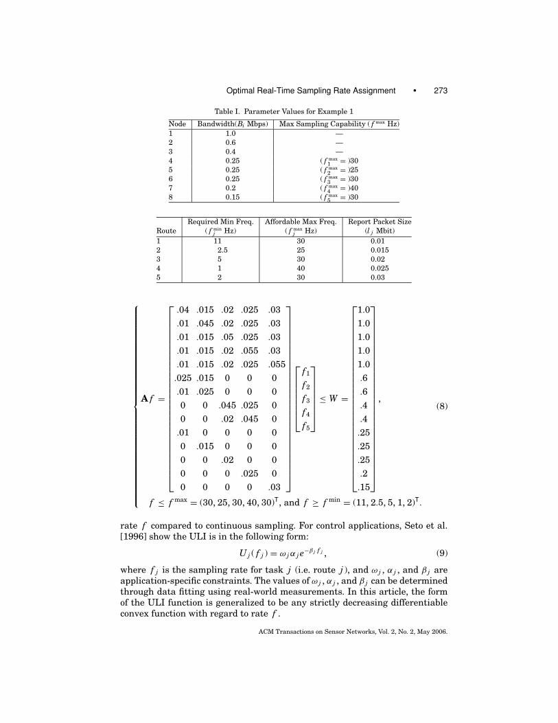
Suppose the numerical values of parameters are as shown in Table I, thenthe complete rate allocation constraints are transformed into (8).

3. OPTIMIZING QOS IN WSN WITH REAL-TIMECONSTRAINTS—MATH MODELING

In this section, we model the optimal sampling rate allocation problem as anonlinear convex optimization problem, using constraints set (5) (6) from theprevious section.

3.1 Utility Loss Index

The base station at the source end of a route periodically samples and reportssensor readings. Let the sampling/reporting rate (or “frequency”) for the j throute be f j . For most applications, the higher the sampling/reporting rate f j ,the higher is the QoS. For example, for control applications, the faster thesampling rate, the better the control performance [Seto et al. 1996]. Ideally,the best performance is achieved if the sampling rate is approaching ∞, that iscontinuous sampling. In practice, this is not achievable, so we use the UtilityLoss Index (ULI) function to capture the performance loss at a discrete sampling



Table I. Parameter Values for Example 1

Node Bandwidth(Bi Mbps) Max Sampling Capability ( f max Hz)

1 1.0 —

2 0.6 —

3 0.4 —

4 0.25 ( f max1

= )30

5 0.25 ( f max2

= )25

6 0.25 ( f max3

= )30

7 0.2 ( f max4

= )40

8 0.15 ( f max5

= )30

Required Min Freq. Affordable Max Freq. Report Packet Size

Route ( f minj Hz) ( f max

j Hz) (l j Mbit)

1 11 30 0.01

2 2.5 25 0.015

3 5 30 0.02

4 1 40 0.025

5 2 30 0.03

⎧⎪⎪⎪⎪⎪⎪⎪⎪⎪⎪⎪⎪⎪⎪⎪⎪⎪⎪⎪⎪⎪⎪⎪⎪⎪⎪⎪⎪⎪⎪⎪⎨⎪⎪⎪⎪⎪⎪⎪⎪⎪⎪⎪⎪⎪⎪⎪⎪⎪⎪⎪⎪⎪⎪⎪⎪⎪⎪⎪⎪⎪⎪⎪⎩

A f =

⎡⎢⎢⎢⎢⎢⎢⎢⎢⎢⎢⎢⎢⎢⎢⎢⎢⎢⎢⎢⎢⎢⎢⎢⎢⎢⎢⎢⎢⎣

.04 .015 .02 .025 .03

.01 .045 .02 .025 .03

.01 .015 .05 .025 .03

.01 .015 .02 .055 .03

.01 .015 .02 .025 .055

.025 .015 0 0 0

.01 .025 0 0 0

0 0 .045 .025 0

0 0 .02 .045 0

.01 0 0 0 0

0 .015 0 0 0

0 0 .02 0 0

0 0 0 .025 0

0 0 0 0 .03

⎤⎥⎥⎥⎥⎥⎥⎥⎥⎥⎥⎥⎥⎥⎥⎥⎥⎥⎥⎥⎥⎥⎥⎥⎥⎥⎥⎥⎥⎦

⎡⎢⎢⎢⎢⎢⎢⎣

f1

f2

f3

f4

f5

⎤⎥⎥⎥⎥⎥⎥⎦

≤ W =

⎡⎢⎢⎢⎢⎢⎢⎢⎢⎢⎢⎢⎢⎢⎢⎢⎢⎢⎢⎢⎢⎢⎢⎢⎢⎢⎢⎢⎢⎣

1.0

1.0

1.0

1.0

1.0

.6

.6

.4

.4

.25

.25

.25

.2

.15

⎤⎥⎥⎥⎥⎥⎥⎥⎥⎥⎥⎥⎥⎥⎥⎥⎥⎥⎥⎥⎥⎥⎥⎥⎥⎥⎥⎥⎥⎦

,

f ≤ f max = (30, 25, 30, 40, 30)T, and f ≥ f min = (11, 2.5, 5, 1, 2)T.

(8)

rate f compared to continuous sampling. For control applications, Seto et al.[1996] show the ULI is in the following form:

U j ( f j ) = ω j α j e−β j f j , (9)

where f j is the sampling rate for task j (i.e. route j ), and ω j , α j , and β j areapplication-specific constraints. The values of ω j , α j , and β j can be determinedthrough data fitting using real-world measurements. In this article, the formof the ULI function is generalized to be any strictly decreasing differentiableconvex function with regard to rate f .



3.2 Mathematical Formulation

Assume each individual ULI function U j ( f j ) is strictly decreasing differen-tiable and convex. Suppose ULIs are additive, the system’s overall ULI isthereby the sum of the ULIs of all individual routes:

∑Nj=1 U j ( f j ). The per-

formance optimization problem becomes:

min( f1,..., f N )

N∑j=1

U j ( f j ) (10)

such that: A f ≤ W (11)

f ≤ f max (12)

f ≥ f min (13)

where A is a constraint matrix with dimension M ×N . M is dependent upon therouting topology of the RTWSN, and N is the number of total routes. We call thisproblem the Multiple Constraints Optimization Problem (MCOP) in contrast toSeto et al. [1996]’s Single Constraint Optimization Problem (SCOP), and wedenote the former as MCOP(U, A, W ).5

The feasible set of MCOP is compact and convex and U j ( f j ) is differen-tiable and convex, therefore MCOP has optimal solutions [Bertsekas 1995].Furthermore, if U j ( f j ) is strictly convex, the optimal solution is unique[Bertsekas 1995].

When M = 1 and there is no constraint set (12), and the ULIs are in the neg-ative exponential form, then MCOP(U, A, W ) becomes SCOP as follows [Setoet al. 1996]:

min( f1,..., f N )

N∑j=1

U j ( f j ) =N∑

j=1

ω j α j e−β j f j (14)

such that: Af ≤ W (15)

f ≥ f min = (f min

1 , . . . , f minN

)T, (16)

where W is the bandwidth (utilization) constraints, and A ∈ R1×N , f ∈ R

N×1,W ∈ R.

Based on the Kuhn-Tucker condition, Seto et al. [1996] provide an algorithmto solve the SCOP problem analytically. MCOP is a generalization of SCOP. Wewill show that the approach for deriving an analytical solution to SCOP is notviable for solving MCOP. To this end, we first prove that the optimal solutionf ∗ of MCOP will make at least one of the constraints in constraint sets (11) and(12) become the equality constraint, and show why it is not viable to tackle theMCOP in an analytical fashion similar to Seto et al. [1996]. In MCOP(U, A, W ),constraint sets (11) and (12) can be combined as:

A′ f ≤ W ′,

where A′ =[

AI

](M+N )×N

, W ′ =[

Wf max

](M+N )×1

. (17)

5Notation used in Kelly et al. [1998].



THEOREM 3.1. MCOP’s optimal solution f ∗, must ensure that at least oneof the (M + N ) constraints A′

i f ∗ ≤ W ′i , i = 1, . . . , (M + N ) reaches equality:

∃i ∈ {1, . . . , M + N } such that A′i f ∗ = W ′

i . Here A′i is the ith row of A′.

PROOF. Please refer to Appendix B for the proof.

Though we know for the optimal rate assignment f ∗, there is at least one isuch that A′

i f ∗ = W ′i , we do not know explicitly which constraints reach equal-

ity. This makes the Kuhn-Tucker based solution method not applicable. In con-trast, the problem discussed in Seto et al. [1996], which is a SCOP (M = 1), ismuch easier because there is only one nontrivial constraint A1 f ∗ ≤ W1, and itis exactly this constraint that should reach equality. In addition to Seto et al.[1996], Rajkumar et al. [1997] proposed a numerical solution. But that solutionis also for a single constraint scenario. In their more recent works, Lee et al.[1999] and Ghosh et al. [2003] studied the scenario under multiple constraints.However, the problem they studied is an integer programming problem, whichis different from the model we will discuss in this article. In Lee et al. [1999], theinteger programming problem is proven to be NP-Hard. Several suboptimal al-gorithms are proposed. According to Ghosh et al. [2003], the one that scales wellis Hierarchical Q-RAM. However, that algorithm requires the division of mul-tiple constraints into independent groups, which is impractical for multi-hopRTWSN (see Section 6.5). Fortunately, as will become clear later, MCOP can besolved with the state-of-art Interior Point Methods [Nesterov and Nemirovsky1994; Ye 1997a] and Internet pricing schemes [Low and Lapsley 1999; Kellyet al. 1998; Kelly 1997].

4. CENTRALIZED SOLUTION METHOD FOR MCOP

In this section, we apply the Interior Point Method (IPM) to solve the MCOPproblem for RTWSN.

Definition 4.1. A Constrained Optimization Problem is expressed asmin{ f (x) : x ∈ Q ⊆ R

n}, where the constraint set Q is defined by multipleequalities and inequalities: Q = {x : h(x) = 0, g (x) ≤ 0}, where h : R

n →R

p; g : Rn → R

q .

Definition 4.2. A Convex Optimization (CO) problem is a constrained opti-mization problem whose objective function f (x) is continuous and convex, andwhose constraint set Q is compact (closed and bounded) and convex.

It’s easy to see that an MCOP is a constrained convex optimization prob-lem with linear constraints. For solving a convex optimization problem, themajor difficulties come from the multiple inequality constraints. Closed formsolutions are generally unavailable. However, IPMs [Nesterov and Nemirovsky1994; Ye 1997a] can solve linear constraint convex optimization problems nu-merically. IPM is a numerical method that iterates in the interior of the solu-tion space defined by constraint set Q to find the optimal solution. IPMs can befurther divided into two subcategories: primal methods and primal-dual meth-ods. Primal-dual methods try to solve the primal and dual optimization prob-lems [Luenberger 1984] together. In practice, the primal-dual methods are more



efficient. The advantages of the interior-point method based numerical solutionincludes: (1) Efficient. IPMs give the correct solution very fast; (2) Multi-hopapplication scenarios: The objective function need not be confined as an expo-nential form as in Seto et al. [1996], but can be a general strictly decreasingdifferentiable convex function.

To solve the MCOP problem, we use optimization library COPL LC [Ye1997b]. It is easy to transform our MCOP problem to the form used by COPL LC.The transformation method can be found in Appendix C. To implement the IPMbased centralized solution, the whole RICH RTWSN elects a central computingnode C, which gathers ULI and constraints information from all the network,carries out the optimization algorithm, and returns the final results.

5. DISTRIBUTED ALGORITHMS FOR OPTIMAL RATE ASSIGNMENT

However, a direct application of IPM results in a centralized solution thatrequires collecting data from each node. This will create a traffic bottleneckaround the central computing node (detailed discussion is in Section 6.5). Toovercome the bottleneck problem, we give a distributed algorithm for solvingthe MCOP. The distributed algorithm lets routers and routes’ end point nodescollaborate to find the optimal rates. The algorithm is based on the recent re-searches of Internet pricing schemes [Low and Lapsley 1999; Kelly et al. 1998;Kelly 1997], especially Low and Lapsley [1999].

The main idea is to impose a price on each constraint in (11)∼(13). Each routewill accumulate its relevant constraints’ prices and solve a local optimizationproblem based on its own ULI function. The result is the next proposed samplingrate for the route (to simplify, we call it rate proposal in the following). Therate proposal is then delivered to each of the route’s routers, where each ofthe route’s relevant constraint updates (imagine each constraint as an activeagent) its price (called constraint price) accordingly. This procedure works inan iterative manner until it converges.

The distributed algorithm has two main attributes:

(1) It converges to the optimal rates of MCOP (Theorem 5.1).

(2) Each route’s computation is only based on local information.

Notations used in the Distributed Algorithm:

s. is the algorithm’s iteration step, s = 0, 1, . . . .p(s). is the updated constraint price vector for each constraint i, i ∈

{1, . . . , M } at iteration step s. p(s) = (p1(s), . . . , pM (s)).f (s). is the updated rate proposal vector for each route j , j ∈ {1, . . . , N } at

iteration step s. f (s) = ( f1(s), . . . , f N (s))T.The Distributed Algorithm:

The distributed algorithm is made up of iterations. Each iteration consistsof two consecutive steps: the Constraint Algorithm, and the Route Algorithm.

At the very beginning of the distributed algorithm, set f (0) = f min, andp(0) ≥ 0.



(1) Constraint AlgorithmDuring iteration s = 1, 2, . . . , for each constraint i(i = 1, . . . , M ):

C1. Receives rate proposal f j (s) from each relevant route j . Route j and con-straint i are relevant if Ai j �= 0.

C2. Computes a new constraint price for itself using the following price updateequation:

pi(s + 1) = [pi(s) + γ ( f i(s) − Wi)]+ (18)

Here f i(s) = Ai f (s), and Ai is the ith row of A. Function [•]+ is defined as[x]+ = max{x, 0}, where x is a real number.

C3. Delivers new price pi(s + 1) to all routes that are relevant to constraint i.

(2) Route AlgorithmDuring iteration s = 1, 2, . . . , for each route j ( j = 1, . . . , N ):

R1. Receives from the network the sum of all the constraints’ prices pj (s) im-posed on this route:

pj (t) =M∑

i=1

pi(s)Ai j (19)

R2. Update the route’s rate proposal f j (s + 1) for the next iteration accordingto the local optimization of:

min U j ( f j ) + f j p j (s)

such that: f minj ≤ f j ≤ f max

j

i.e. f j (s + 1) = arg minf min

j ≤ f j ≤ f maxj

(U j ( f j ) + f j p j (s)) (20)

The iteration of Constraint and Route Algorithms stops until the predefinedconvergence criterion is reached. For example, when both of the following cri-teria are met.

‖ f (s) − f (s − 1)‖n ≤ ε f , (21)

‖q(s) − q(s − 1)‖n ≤ εq , (22)

where f (s) = ( f1(s), f2(s), . . . , f N (s))T, q(s) = (p1(s), p2(s), . . . , pN (s))T. ε f > 0and εp > 0 are sufficiently small real numbers. ‖v‖n denotes the nth-norm ofvector v = (v1, . . . , vk). If n = 1, ‖v‖1 = max(vi), i ∈ {1, . . . , k}. If n ∈ Z

+, then

‖v‖n = (∑k

i=1 vni )

1n .

Now we prove the convergence and correctness of the above iterative algo-rithm. This is summarized in Theorem 5.1. First, we give the assumptions andnotations to be used.

Assumptions:

A1. The feasibility condition holds for each constraint i(i = 1, . . . , M ), suchthat

∑Nj=1 Ai j f min

j ≤ Wi.

A2. For each route j , on the interval I j = [ f minj , f max

j ], the utility function U j

is strictly decreasing, strictly convex, and twice continuously differentiable.



A3. The curvature of U j for each route satisfies the following condition on

I j = [ f minj , f max

j ], ∃α j , such that U ′′j ( f j ) ≥ 1

α j> 0, for all f j ∈ I j .

Notations Used in Theorem 5.1:

� L( j ) = ∑Mi=1 Ai j . It is the column sum of A;

� L = max j=1,...,N {|L( j )|}, which is the maximum absolute value of the columnsum of A;

� S(i) = ∑Nj=1 Ai j . It is the row sum of A;

� S = maxi=1,...,M {|S(i)|}, which is the maximum absolute value of the row sumof A;

� α = max j=1,...,N {α j }. α is the upper bound on 1U ′′

j ( f j ), j = 1, . . . , N .

THEOREM 5.1. Suppose assumptions A1 ∼ A3 hold and the step size γ satis-fies 0 < γ < 2/(αLS). Then starting from any initial rates f min ≤ f (0) ≤ f max

and prices p(0) ≥ 0, the sequence {( f (s), p(s))} generated by the above distributedalgorithm will converge to a accumulation point ( f ∗, p∗), and f ∗ is the solutionof MCOP(U, A, W ).

PROOF. See Appendix D.

6. EVALUATION

In this section, we shall present the simulation results and discuss the trade-offs between the centralized algorithm and the distributed algorithm, showingwhich is more appropriate in what situations. We also show that the distributedalgorithm has the desirable incremental adjustment property.

6.1 Implementation

First let us look at the real-world feasibility of RICH architecture. Real-world DSSS Chip-Sets consist of multiple parallel independent transmittersand receivers are already available. For example, the QualComm CSM2000chipset [Qualcomm 2004a], originally designed for low-cost lightweight cellu-lar base stations, supports eight parallel users, which is enough for the seven-transceiver RICH architecture. Higher performance chipsets can be Qual-Comm CSM5000 [Qualcomm 2004b], CSM5500 [Qualcomm 2004c] and so on,which can be easily reconfigured to build RICH base stations, providing noless than 1.8Mbps data bandwidth for each of the seven transceivers. Thesizes and power consumption of these chip sets are also satisfactorilly small.For example, a CSM5500 chip complies with BGA560 packaging, which is35×35×2.5 mm in dimension; and is of 3 ∼ 3.6 volt I/O voltage and 1.8 volt corevoltage.

Based on the above real-world parameters, we carry out simulation usingJ-Sim [DRCL 2004]. The centralized algorithm is straightforward. To simulatethe distributed algorithm, we need to devise a network protocol that matchesthe algorithm described in Section 5, which is as following:



Network Protocol for Distributed Algorithm:The protocol is carried out in iterations, each iteration s consists of two steps:

Step 1. Each constraint’s price is updated by the router that creates that con-straint based on (18). Next, each of these updated prices must be propa-gated to all the relevant routes. To do that, each route’s source end sendsan empty packet toward the destination end. The packet’s payload is justone floating-point number (4 bytes), dedicated to carry the total price pj (s),where j refers to the j th route. As this packet travels toward the destina-tion along the route, on each hop, it will accumulate onto pj (s) all relevantconstraints’ prices maintained by the local router. When the packet reachesthe destination end, the total price pj (s) is obtained.

Step 2. After Step 1, each route’s destination end carries out the route algorithm(20) to update the sampling rate proposal. Then the destination end sendsanother packet towards the source end, to notify every router along thisroute about the updated sampling rate proposal. This packet’s payload isalso just one floating-point number (4 bytes), which is enough to carry theupdated sampling rate proposal.

If the payload of the control traffic is piggybacked to the data traffic, it willadd a 4 bytes overload. If the control traffic is sent separately from the datatraffic, it can be encoded into a 16 byte packet. Within this 16 byte packet, 4bytes are the control payload, 4 bytes are for the source address, 4 bytes arefor the destination address, and the remaining 4 bytes are for other purposes,such as checksum and so on. In the following, we discuss the separate controlmessage scheme, that is, the distributed algorithm incurs a 16 byte packet inStep 1 and Step 2 respectively for each route.

For the distributed algorithm, we also assume all the involved routes ofthe RTWSN are coarse-grain synchronized in the sense that in each iteration,all the routes finish Step 1 and then move on to Step 2; and when all theroutes finish Step 2, they move on to the next iteration. This can be achieved,for examples, by synchronizing all the nodes and starting each step at timekTstep, where k ∈ Z, and Tstep is the empirical upper bound of end-to-end packettravel time along the network diameter, assuming there is a specified upperbound on network diameter. The GPS System [Getting 1993] can already pro-vide global time synchronization with an accuracy of within 0.25 msec [ExitConsulting 2004], which is enough for our application. For example, in oursimulation setup, a synchronization granularity of 2msec is enough for thetestbed.

6.2 Numerical Example of the Centralized and the Distributed Algorithm

First both the centralized and distributed algorithms are applied to the scenariodiscussed in Example 1 of Section 2.2. The setup involves 5 routes. The ULIfunction for each route j is in the form of ω j α j e−β j f j , so the MCOP(U, A, W )’s

total ULI (the objective function) is:∑5

j=1 U j ( f j ) = ∑5j=1 ω j α j e−β j f j , with pa-

rameters shown in Table II. These parameters are taken from those reportedin Sha et al. [2000]. Constraints are listed in equation (8).



Table II. Parameters for

ULI in Example 1

Route α j β j ω j

1 0.66 0.3 1

2 0.66 1.0 2

3 0.66 0.5 3

4 0.66 0.7 4

5 0.66 0.3 5

Fig. 5. Rate proposal update trace.

Using the centralized algorithm and the COPL LC package [Ye1997b], by 14 iterations, the optimal solution is derived: f ∗

central =(12.35, 6.58, 5.70, 5.73, 5.00)T, with an optimal value of 0.916.6

For the distributed algorithm, we choose the initial values to be f (0) =f min, p(0) = (0, 0, 0, 0, 0, 0, 0, 0, 0, 0, 0, 0, 0, 0) and γ = 2 × 10−7. The networkparameter settings follow Table I. The convergence criteria are described byequations (21) and (22), where we pick ε f = 1×10−9 and εq = 1×10−9. The rateproposal update trace is shown in Figure 5. The trace shows that the algorithmconverges in a short time (no more than 9.48sec). The converged rate proposalvalue is: f ∗

distributed = (12.35, 6.58, 5.70, 5.73, 5.00)T, which matches the resultsobtained from the centralized algorithm.

It is worth noting that, for many RTWSN applications, it is not necessary toderive the exact optimum sampling rate. Instead, getting a quasi-optimum ina relatively shorter time is often preferrable. In Table III, the convergence timefor each route with certain error bound is listed. We see that if coarser errorbound is allowed, the convergence time is even shorter.

6.3 Monte Carlo Simulation on Convergence Speed

In order to give a feeling of how fast the distributed algorithm converges, thefollowing Monte Carlo simulation is carried out:

6The primal objective values reported in the 14 iterations are {1.649, 1.339, 1.237, 1.072, 0.834,

0.504, 0.649, 0.683, 0.792, 0.899, 0.915, 0.916, 0.916, 0.916}.



Table III. Convergence Time

Route 1 2 3 4 5

Convergence Time (CT) (sec) 6.58 5.80 5.59 5.66 9.48

CT when ± 1% error is allowed (sec) 1.79 1.39 0.45 0.27 2.73

CT when ± 5% error is allowed (sec) 0.74 0.46 0.23 0.13 1.6

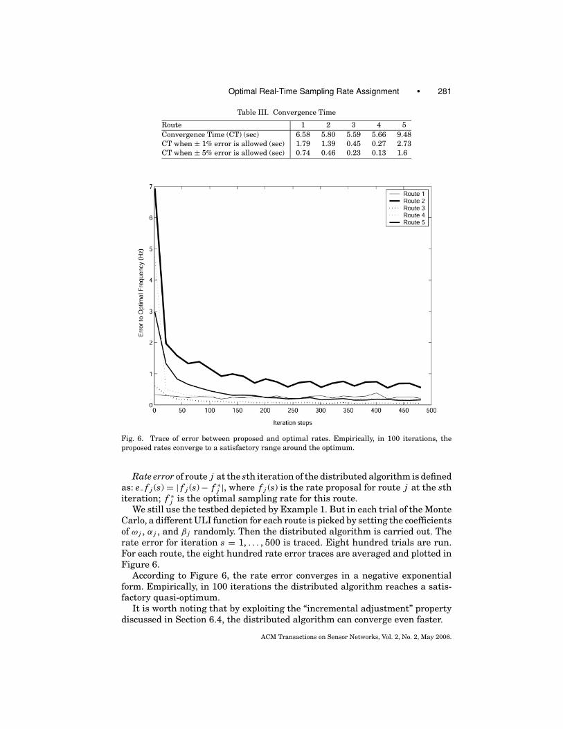
Fig. 6. Trace of error between proposed and optimal rates. Empirically, in 100 iterations, the

proposed rates converge to a satisfactory range around the optimum.

Rate error of route j at the sth iteration of the distributed algorithm is definedas: e f j (s) = | f j (s) − f ∗

j |, where f j (s) is the rate proposal for route j at the sthiteration; f ∗

j is the optimal sampling rate for this route.We still use the testbed depicted by Example 1. But in each trial of the Monte

Carlo, a different ULI function for each route is picked by setting the coefficientsof ω j , α j , and β j randomly. Then the distributed algorithm is carried out. Therate error for iteration s = 1, . . . , 500 is traced. Eight hundred trials are run.For each route, the eight hundred rate error traces are averaged and plotted inFigure 6.

According to Figure 6, the rate error converges in a negative exponentialform. Empirically, in 100 iterations the distributed algorithm reaches a satis-factory quasi-optimum.

It is worth noting that by exploiting the “incremental adjustment” propertydiscussed in Section 6.4, the distributed algorithm can converge even faster.



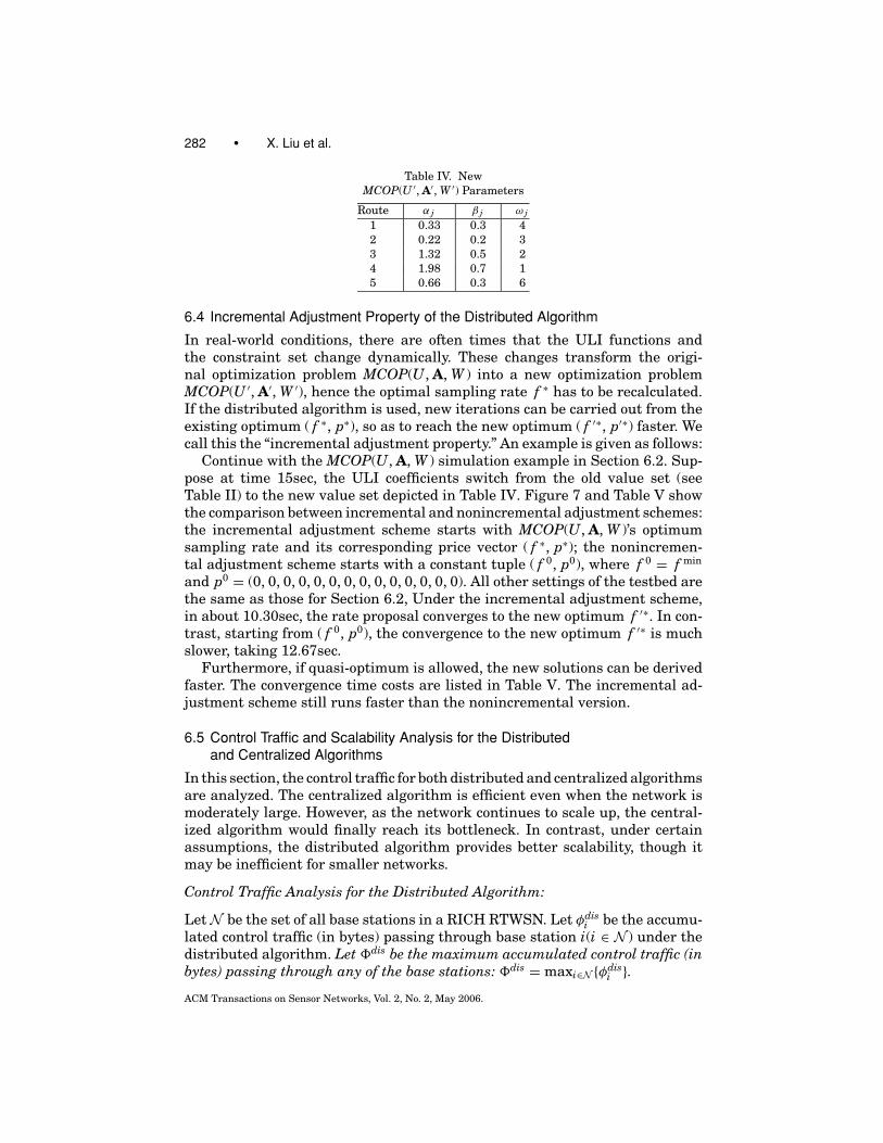
Table IV. New

MCOP(U ′, A′, W ′) Parameters

Route α j β j ω j

1 0.33 0.3 4

2 0.22 0.2 3

3 1.32 0.5 2

4 1.98 0.7 1

5 0.66 0.3 6

6.4 Incremental Adjustment Property of the Distributed Algorithm

In real-world conditions, there are often times that the ULI functions andthe constraint set change dynamically. These changes transform the origi-nal optimization problem MCOP(U, A, W ) into a new optimization problemMCOP(U ′, A′, W ′), hence the optimal sampling rate f ∗ has to be recalculated.If the distributed algorithm is used, new iterations can be carried out from theexisting optimum ( f ∗, p∗), so as to reach the new optimum ( f ′∗, p′∗) faster. Wecall this the “incremental adjustment property.” An example is given as follows:

Continue with the MCOP(U, A, W ) simulation example in Section 6.2. Sup-pose at time 15sec, the ULI coefficients switch from the old value set (seeTable II) to the new value set depicted in Table IV. Figure 7 and Table V showthe comparison between incremental and nonincremental adjustment schemes:the incremental adjustment scheme starts with MCOP(U, A, W )’s optimumsampling rate and its corresponding price vector ( f ∗, p∗); the nonincremen-tal adjustment scheme starts with a constant tuple ( f 0, p0), where f 0 = f min

and p0 = (0, 0, 0, 0, 0, 0, 0, 0, 0, 0, 0, 0, 0, 0). All other settings of the testbed arethe same as those for Section 6.2, Under the incremental adjustment scheme,in about 10.30sec, the rate proposal converges to the new optimum f ′∗. In con-trast, starting from ( f 0, p0), the convergence to the new optimum f ′∗ is muchslower, taking 12.67sec.

Furthermore, if quasi-optimum is allowed, the new solutions can be derivedfaster. The convergence time costs are listed in Table V. The incremental ad-justment scheme still runs faster than the nonincremental version.

6.5 Control Traffic and Scalability Analysis for the Distributedand Centralized Algorithms

In this section, the control traffic for both distributed and centralized algorithmsare analyzed. The centralized algorithm is efficient even when the network ismoderately large. However, as the network continues to scale up, the central-ized algorithm would finally reach its bottleneck. In contrast, under certainassumptions, the distributed algorithm provides better scalability, though itmay be inefficient for smaller networks.

Control Traffic Analysis for the Distributed Algorithm:

Let N be the set of all base stations in a RICH RTWSN. Let φdisi be the accumu-

lated control traffic (in bytes) passing through base station i(i ∈ N ) under thedistributed algorithm. Let dis be the maximum accumulated control traffic (inbytes) passing through any of the base stations: dis = maxi∈N {φdis

i }.ACM Transactions on Sensor Networks, Vol. 2, No. 2, May 2006.


Fig. 7. Illustration of incremental adjustment property.

Table V. Convergence Time of MCOP(U ′, A′, W ′)

Route 1 2 3 4 5

starts with Convergence Time (CT) (sec) 8.67 7.68 6.98 7.32 10.30

( f ∗, p∗) CT when ±1% error is allowed (sec) 0.01 1.13 0.25 0.07 1.24

CT when ±5% error is allowed (sec) 0.01 0.05 0.03 0.02 0.15

starts with Convergence Time (CT) (sec) 11.04 10.05 9.35 9.69 12.67

( f 0, p0) CT when ±1% error is allowed (sec) 0.002 3.51 1.25 1.61 3.61

CT when ±5% error is allowed (sec) 0.002 1.93 0.03 0.39 2.01

Let R be the set of all routers (RICH base stations that serve as routers) inthe same RICH RTWSN. Let dr be the number of routes passing through routerr(r ∈ R): the out-degree of router r. Let D be the maximum number of routespassing through any routers: D = maxr∈R{dr}.

During each iteration, in Step 1, totally dr control packets pass throughrouter r. In Step 2, totally dr packets pass through router r. Without loss ofgenerality, we assume all control packets have 12 bytes of headers. As men-tioned previously, each packet’s payload length is 4 bytes. Therefore the total



control traffic passing through each router r during each iteration is 32dr bytes,we therefore have the following proposition:

PROPOSITION 6.1. For any base station i ∈ N , during each distributed al-gorithm iteration, the number of control packets-passing through it is no morethan 32D bytes.

According to our simulation results in Section 6.3, the distributed algorithmusually converges or reaches a very good approximation in K ≤ 100 steps(exploiting the incremental adjustment property discussed in Section 6.4, orallowing quasi-optimum, the number of iterations may be even less). Henceafter all the iterations, the accumulated control traffic passing through anyrouter is no more than 32K D. That is, for any node i ∈ N , φdis

i ≤ 32K D ≤32 × 100D = 3200D (byte). Therefore we have:

dis ≤ 3200D (23)

dis = O(D). (24)

Traffic Load Analysis for Centralized Algorithm:

Let N be the set of all base stations in a RICH RTWSN. Let φceni be the accumu-

lated control traffic passing through base station i(i ∈ N ) under the centralizedalgorithm. Let cen be the maximum accumulated control traffic passing throughany of the base stations: cen = maxi∈N {φcen

i }.Suppose the total number of routes in a RICH RTWSN is total. Under the

centralized algorithm, each route at least needs to send the central computingnode C its ULI information together with at least one constraint. Without lossof generality, we suppose each ULI function is expressed by 3 floating pointnumbers (12 bytes) and each constraint is at least represented by 2 floatingpoint numbers (8 bytes). To be consistant, we still assume the control packetheader has 12 bytes. Thus the accumulated control traffic payload at node C isφcen

C ≥ 32total; φcenC = �(total). Because cen ≥ φcen

C , we have:

cen = �(total). (25)

One may argue that the routes in a RICH RTWSN may not be all directlyor indirectly connected, but rather partitioned into several disjoint maximalsubgraphs (routes within each maximal subgraph are directly or indirectly con-nected). So that there need not be ONE central computing node. Each maximalsubgraph can elect its own central computing node, which takes charge of theoptimal sampling rate planning for, and only for, the routes within that max-imal subgraph. In this case, let G be the set of all maximal subgraphs, for aspecific maximal subgraph g ∈ G, let g be the number of routes in g . Let Cg

be the elected central computing node for g . Because of the same reasoningwith which we derived (25), we have φcen

Cg≥ 32g . By the definition of cen,

we still have cen ≥ φcenCg

≥ 32g . That is: ∀g ∈ G, cen ≥ 32g , which implies

cen ≥ maxg∈G{32g }. Let = maxg∈G{g }, the maximum number of directly



or indirectly connected routes of the whole RTWSN; then we have:

cen ≥ 32

i.e. cen = �(). (26)

In the following simulation for wide area monitoring, we shall show ≈ total,(26) is empirically equivalent to (25). We shall also show dis is empirically in-sensitive to the scale of the RICH RTWSN while cen increases at least quadrati-cally with the scale of the RICH RTWSN. This means the centralized algorithm’scentral computing node is a control message exchanging bottleneck. Hence thecentralized algorithm does not scale up well while the distributed algorithmdoes.

Comparison of the Distributed and Centralized Algorithms:

In many cases, even for moderately large networks, the centralized algorithm isefficient enough. But there are certain cases where the distributed algorithm ismore scalable than the centralized algorithm. An example scenario is as follows:

Suppose all routes are desseminated in a square area of l × l km2, where lis the square edge length. The square area deploys a RICH RTWSN cellulardivision with a hexagon cell edge length of 0.1km. All routes between basestations are unicast, and we assume the network diameter is upper boundedby a fixed constant, which, without loss of generality, is set to 10. Specifically,the source end base stations of all routes are uniformly distributed across thesquare area with density ρ = 10/km2; and the destination end is also uniformlydistributed within 10 hops from the source end. This also implies the totalnumber of routes is ρl2. The route is determined by the source/destination endand a simple geographical routing protocol that always forwards the packetcloser to the destination in each hop.

For each RICH RTWSN scale (l = 5, . . . , 100(km)), thirty trials are carriedout. In each trial, ρl2 routes are generated according to the previous descrip-tion; then the maximum number of routes passing through any router (D),and the maximum number of directly or indirectly connected routes () arecounted. The results are shown in Table VI. For ease of comparision, we plotthe same data in Figure 8. We can see from Figure 8, D is bounded by a relativelysmall constant, insensitive to the network scale l , while rises in a roughly l2

speed.7

According to (24) and (26), dis = O(D) and cen = �(). Therefore for thedistributed algorithm, the maximum per-base station accumulated control traf-fic (dis) is upper bounded by D, and D is insensitive to the scale of the network.In contrast, for the centralized algorithm, the maximum per-base station accu-mulated control traffic (cen) is lower bounded by , and is growing quadrat-ically with the network scale l . The underlying reason is that for the cen-tralized algorithm, the control traffic is bottlenecked at the central computingnode, while for the distributed algorithm, the control traffic is evenly the dis-tributed among all the nodes. Hence, the distributed algorithm shows betterscalability.

7In other scenarios, the sensitivity analysis of D to network scale is left for future research.



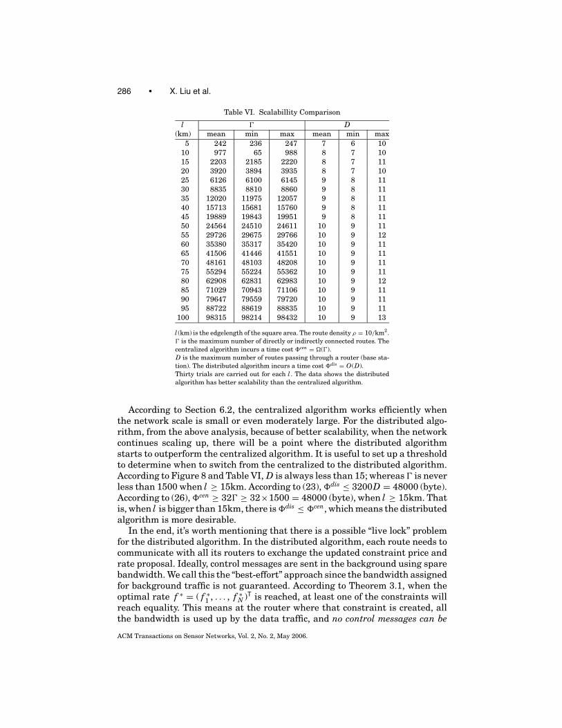
Table VI. Scalabillity Comparison

l D(km) mean min max mean min max

5 242 236 247 7 6 10

10 977 65 988 8 7 10

15 2203 2185 2220 8 7 11

20 3920 3894 3935 8 7 10

25 6126 6100 6145 9 8 11

30 8835 8810 8860 9 8 11

35 12020 11975 12057 9 8 11

40 15713 15681 15760 9 8 11

45 19889 19843 19951 9 8 11

50 24564 24510 24611 10 9 11

55 29726 29675 29766 10 9 12

60 35380 35317 35420 10 9 11

65 41506 41446 41551 10 9 11

70 48161 48103 48208 10 9 11

75 55294 55224 55362 10 9 11

80 62908 62831 62983 10 9 12

85 71029 70943 71106 10 9 11

90 79647 79559 79720 10 9 11

95 88722 88619 88835 10 9 11

100 98315 98214 98432 10 9 13

l (km) is the edgelength of the square area. The route density ρ = 10/km2.

is the maximum number of directly or indirectly connected routes. The

centralized algorithm incurs a time cost cen = �().

D is the maximum number of routes passing through a router (base sta-

tion). The distributed algorithm incurs a time cost dis = O(D).

Thirty trials are carried out for each l . The data shows the distributed

algorithm has better scalability than the centralized algorithm.

According to Section 6.2, the centralized algorithm works efficiently whenthe network scale is small or even moderately large. For the distributed algo-rithm, from the above analysis, because of better scalability, when the networkcontinues scaling up, there will be a point where the distributed algorithmstarts to outperform the centralized algorithm. It is useful to set up a thresholdto determine when to switch from the centralized to the distributed algorithm.According to Figure 8 and Table VI, D is always less than 15; whereas is neverless than 1500 when l ≥ 15km. According to (23), dis ≤ 3200D = 48000 (byte).According to (26), cen ≥ 32 ≥ 32×1500 = 48000 (byte), when l ≥ 15km. Thatis, when l is bigger than 15km, there is dis ≤ cen, which means the distributedalgorithm is more desirable.

In the end, it’s worth mentioning that there is a possible “live lock” problemfor the distributed algorithm. In the distributed algorithm, each route needs tocommunicate with all its routers to exchange the updated constraint price andrate proposal. Ideally, control messages are sent in the background using sparebandwidth. We call this the “best-effort” approach since the bandwidth assignedfor background traffic is not guaranteed. According to Theorem 3.1, when theoptimal rate f ∗ = ( f ∗

1 , . . . , f ∗N )T is reached, at least one of the constraints will

reach equality. This means at the router where that constraint is created, allthe bandwidth is used up by the data traffic, and no control messages can be



Fig. 8. Scalability Comparison. l (km) is the edgelength of the square area. The route density

ρ = 10/km2. is the maximum number of directly or indirectly connected routes. The centralized

algorithm incurs a time cost cen = �(). D is the maximum number of routes passing through

any router (base station). The distributed algorithm incurs a time cost dis = O(D). Thirty trials

are carried out for each l . The results shows the distributed algorithm has better scalability than

the centralized algorithm.

sent through that router any more! This causes a “live lock” problem since ifthere is future need for exchanging control messages, the saturated router canno longer participate.

A solution to the “live lock” problem is to preserve a small amount of dedicatedbandwidth for exchanging the control messages. According to Proposition 6.1,the maximum amount of control message payload bytes passing through eachRICH RTWSN node during each iteration is no more than 32D, where D is themaximum number of routes passing through any router in the whole RTWSN.Figure 8 and Table VI show when the maximum route length and density ofroutes in the RTWSN are fixed, and the end points of routes are uniformly thedistributed; empirically, D is bounded by a constant, which can be estimatedvia simulation. Therefore, the bandwidth to be reserved for control messageexchange can be planned accordingly. For example, according to Figure 8 andTable VI, D is empirically bounded by 15. Therefore each iteration causes a con-trol traffic of 32 × 15 = 480 bytes. If 100 iterations are needed to get the result,and the distributed algorithm is supposed to finish in 4 seconds, then the con-trol traffic bandwidth should be 480 × 8 × 100/4 = 96 (kbps). Note according toSection 6.1, a RICH base station can achieve 1.8Mbps transmitting bandwidthwith lightweight hardware. Also note the above bound is based on worst caseanalysis. In practical applications, if more detailed network information, suchas the number of routes passing through each router is available, then differentrouter nodes can reserve different bandwidth based on this information.



Fig. 9. DSSS modulation/demodulation process: a simplified view.

7. CONCLUSIONS AND FUTURE WORK

In this article, we study the optimal sampling rate assignment in RTWSN, andformalize it into a nonlinear optimization problem. By using the state-of-artmethods in optimization, two solutions are given. One is in a the centralizedfashion, the other is in a the distributed fashion. Our solutions can handlemulti-hop routing scenarios, which are not covered by previous research. Wecompare the trade-offs between the centralized and the distributed algorithmsunder different situations. Specifically, we quantitatively analyze the node-wisecontrol traffic under both algorithms. We show that though the centralizedalgorithm works efficiently with small and even moderately large RTWSNs,it has a bottleneck problem, which limits its scalability. On the other hand,the distributed algorithm is a better choice for large-scale RTWSN and hasthe desirable incremental adjustment property. Also, the convergence of thedistributed algorithm is guaranteed and empirically shown to be fast. Notethat using the GPS for synchronization in the distributed algorithm is not anobligation; an asynchronous algorithm can be designed, for example, similar tothe asynchronous flow control algorithm in Low and Lapsley [1999]. However,an asynchronous algorithm usually converges, more slowly.

Our ongoing research topics include: (1) Integrating QoS optimization anderror modeling for WSN; (2) Theoretical analysis of the distributed algorithm’sconvergence rate for specific WSN applications; (3) ULI function formulationbased on stochastic models.

A. A BRIEF TUTORIAL ON DSSS-CDMA

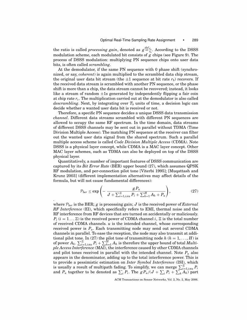
DSSS is a physical layer baseband modulation/demodulation scheme for dig-ital communication. Without loss of generality, we assume digital “1” and “0”are represented by +1 and −1 (volt) rectangular pulses. Unlike conventionalbaseband modulation schemes, where each bit is represented with a single +1or −1 pulse, DSSS multiplies a Pseudo Noise (PN) sequence onto the stream ofuser data bits, as shown in Figure 9.

The PN sequence is also a sequence of ±1 rectangular pulses, with a +1 pulserepresenting digit “1” and a −1 pulse for digit “0”. Each digit of a PN sequenceis called a chip. The number of PN chips generated per second is called chiprate, represented by rc; chip duration Tc is defined as Tc

def= 1rc

. Correspondingly,

the number of data bits generated per second is called bit rate, represented

by rb, and bit duration Tbdef= 1

rb. Usually rc is a positive integer multiple of rb;



the ratio is called processing gain, denoted as gdef= rc

rb. According to the DSSS

modulation scheme, each modulated bit consists of g chips (see Figure 9). Theprocess of DSSS modulation: multiplying PN sequence chips onto user databits, is often called scrambling.

At the demodulator, if the same PN sequence with 0 phase shift (synchro-nized, or say, coherent) is again multiplied to the scrambled data chip stream,the original user data bit stream (the ±1 sequence at bit rate rb) recovers. Ifthe received data stream is scrambled with another PN sequence, or the phaseshift is more than a chip, the data stream cannot be recovered; instead, it lookslike a stream of random ±1s generated by independently flipping a fair coinat chip rate rc. The multiplication carried out at the demodulator is also calleddescrambling. Next, by integrating over Tb units of time, a decision logic candecide whether a wanted user data bit is received or not.

Therefore, a specific PN sequence decides a unique DSSS data transmissionchannel. Different data streams scrambled with different PN sequences areallowed to occupy the same RF spectrum. In the time domain, data streamsof different DSSS channels may be sent out in parallel without TDMA (TimeDivision Multiple Access). The matching PN sequence at the receiver can filterout the wanted user data signal from the shared spectrum. Such a parallelmultiple access scheme is called Code Division Multiple Access (CDMA). NoteDSSS is a physical layer concept, while CDMA is a MAC layer concept. OtherMAC layer schemes, such as TDMA can also be deployed on top of the DSSSphysical layer.

Quantitatively, a number of important features of DSSS communication arecaptured by its Bit Error Rate (BER) upper bound (27), which assumes QPSKRF modulation, and per-connection pilot tone [Viterbi 1995]; [Muqattash andKrunz 2003] (different implementation alternatives may affect details of theformula, but will not cause fundamental differences):

Pber ≤ exp

(− g Pu

J + ∑ i=1,i �=u Pi + ∑H

h=1 Ah + Pu

), (27)

.where Pber is the BER; g is processing gain; J is the received power of ExternalRF Interference (EI), which specifically refers to EMI, thermal noise and theRF interference from RF devices that are turned on accidentally or maliciously.Pi (i = 1 . . . ) is the received power of CDMA channel i, is the total numberof received CDMA channels. u is the intended channel, whose correspondingreceived power is Pu. Each transmitting node may send out several CDMAchannels in parallel. To ease the reception, the node may also transmit at addi-tional pilot tone. In (27) the pilot tone of transmitting node h (h = 1, . . . , H) isof power Ah.

∑ i=1,i �=u Pi + ∑H

h=1 Ah is therefore the upper bound of total Multi-ple Access Interference (MAI), the interference caused by other CDMA channelsand pilot tones received in parallel with the intended channel. Note Pu alsoappears in the denominator, adding up to the total interference power. This isto provide a pessimistic estimation on Inter Symbol Interference (ISI), whichis usually a result of multipath fading. To simplify, we can merge

∑ i=1,i �=u Pi

and Pu together to be denoted as∑

i Pi. The g Pu/(J + ∑i Pi + ∑

h Ah) part



shows the effective SNR for the intended channel, where J + ∑i Pi + ∑

h Ah

represents the upper bound of noise power and g Pu represents effective signalpower. The bigger the SNR, the smaller the probability of bit error Pber. WhenPber is below a certain threshold �ber, the wireless communication is acceptablefor real-time communication. Therefore, to maintain a real-time DSSS-CDMAchannel in fact means to maintain the SNR of the channel from dropping belowan acceptable threshold �snr.

(27) implies that the SNR of the intended channel can be raised by increas-ing the processing gain g . Meanwhile, g is defined as the ratio of chip rate

and bit rate: gdef= rc/rb. Usually, chip rate rc is fixed by hardware because of the

multipath effect and hardware cost constraints [Price and Green 1958]; [Viterbi1995], therefore raising processing gain means slowing down user data bit raterb. DSSS hereby provides a mechanism to leverage between SNR and data bitrate.

B. PROOF OF THEOREM 3.1

Using Lagrangian multipliers λ j , j = 1, . . . , N , and μi, i = 1, . . . , M + N , wecan write the Kuhn-Tucker condition of MCOP(U, A, W ) as:

dU j ( f ∗j )

df j+ μ1A′

1 j + . . . + μ(M+N )A′(M+N ) j − λ j = 0, (28)

where ( j = 1, . . . , N )

f minj − f ∗

j ≤ 0 (29)

λ j(

f minj − f ∗

j

) = 0 (30)

N∑j=1

A′i j f ∗

j ≤ W ′i , (i = 1, . . . , M + N ) (31)

μi

(N∑

j=1

A′i j f ∗

j − W ′i

)= 0 (32)

μi ≥ 0, λ j ≥ 0, (i = 1, . . . , M + N , j = 1, . . . , N ) (33)

Suppose for all i = 1, . . . , M + N ,∑N

j=1 A′i j f ∗

j < W ′i , then from (32), we know

μi = 0. ThendU j ( f ∗

j )

df j+μ1A′

1 j + . . .+μ(M+N )A′(M+N ) j −λ j = dU j ( f ∗

j )

df j−λ j < 0, since

dU j ( f ∗j )

df j< 0. This contradicts equation (28). So we know Theorem 3.1 holds.

C. CONVERSION OF MCOP TO COPL LC

The original COPL LC package is used to solve the problem of equality con-straints as follows:

min g (x)

such that: T x = b, x ≥ 0

where A ∈ Rm×n, b ∈ R

m



This is NOT the form of our problem formulation of MCOP. We have to dosome transformations to transform MCOP into the framework of COPL LC.Here, we use the combined constraints set (17) of MCOP:

min( f1,... , f N )

N∑j=1

U j ( f j ) (10)

such that: A′ f ≤ W ′ (17)

where A′ =[AI

](M+N )×N

, W ′ =[

Wf max

](M+N )×1

.

f ≥ f min (13)

First, we let f j = f j − f minj , so that the constraints f j ≥ f min

j ⇔ f j ≥ 0.

We also add a slack variable y = ( y1, . . . , yM+N )T, so that

A′ f ≤ W ′ ⇔ A′ f + y = W ′, y ≥ 0

⇔ A′ f + y = W ′ − A′ f min, y ≥ 0.

MCOP is thereby transformed to the following form:

min( f1,..., f N )

N∑j=1

U j ( f j )

such that: f j ≥ 0( j = 1, . . . , N )

y ≥ 0N∑

j=1

A′i j f j + yi = W ′

i −N∑

j=1

A′i j f min

j ,

(where i = 1, . . . , M + N ).

This is in the form of COPL LC. To see this, simply let x = [ f1, . . . ,f N , y1, . . . , yM+N ]T, T = [A′

(M+N )×N |I(M+N )×(M+N )], where I(M+N )×(M+N ) is the

(M + N ) × (M + N ) identity matrix and b = W ′ − A′ f min.

D. PROOF OF THEOREM 5.1

First by defining I j = [ f minj , f max

j ] and V (•) = −U (•), we can rewrite theMCOP(U, A, W ) as:

Primary: max f j ∈I j

∑Nj=1 Vj ( f j ) (34)

such that:∑N

j=1 Ai j f j ≤ Wi (i = 1, . . . , M ). (35)

We call this constraint optimization problem the Primary problem. The fol-lowing proof follows Low and Lapsley’s result in Low and Lapsley [1999] withmodifications for our problem.



Let’s first convert the Primary problem to its dual form.Define the Lagrangian with multipliers vector p for the Primary problem as:

L( f , p) =N∑

j=1

Vj ( f j ) −M∑

i=1

pi

(N∑

j=1

Ai j f j − Wi

)

=N∑

j=1

(Vj ( f j ) − f j

M∑i=1

Ai j pi

)+

M∑i=1

piWi.

Notice the first term is separable in f j , and hence:

maxf j ∈I j

N∑j=1

(Vj ( f j ) − f j

M∑i=1

Ai j pi

)=

N∑j=1

maxf j ∈I j

(Vj ( f j ) − f j

M∑i=1

Ai j pi

). (36)

Then, by defining the objective function:

D(p) = maxf j ∈I j

L( f , p)

=N∑

j=1

Bj (pj ) +M∑

i=1

piWi,

where

Bj (pj ) = maxf j ∈I j

(Vj ( f j ) − f j p j ), (37)

pj =M∑

i=1

Aij pi. (38)

The dual problem is:

Dual: minp≥0

D(p). (39)

We call the unique optimizer of (37), f j (pj ). From the Kuhn-Tucker theorem,it is easy to see:

f j (pj ) = [V ′−1

j (pj )] f max

j

f minj

, (40)

where [z]ba = min{max{z, a}, b}, V ′−1

j (•) represents the inverse of derivativefunction V ′

j (•) (with respect to f j ).The three Lemmas given below are used in the proof of Theorem 5.1.

LEMMA D.1. Under assumptions A1 and A2, the dual objective function D(p)is convex, lower bounded, and continuously differentiable.



PROOF. Directly follow assumption A1, A2.

For any price vector p, define β j (p) by

β j (p) ={

1−V ′′

j ( f j (p))if V ′

j

(f max

j

) ≤ pj ≤ V ′j

(f min

j

)0 otherwise.

(41)

Here, f j (p) is the unique maximizer of (37), which is defined in equation(40). Let B(p) = Diag (β j (p)), ( j = 1, . . . , N ) be the N × N diagonal matrix.

Note from assumption A3, we know for ∀p ≥ 0, 1−V ′′

j ( f j (p))= 1

U ′′j ( f j (p))

≤ α j , so

0 ≤ β j (p) ≤ α j ≤ ∞. (42)

LEMMA D.2. Under assumption A1, A2, the Hessian matrix of D is given by∇2 D(p) = AB(p)AT, where it exists.

PROOF. Let ∂ f∂p (p) denote the N × M Jacobian matrix whose ( j , i) element is

∂ f j

∂pi(p). When it exists,

∂ f j

∂pi(p) =

{ Ai j

V ′′j ( f j (p))

if V ′j

(f max

j

) ≤ pj ≤ V ′j

(f min

j

)0 otherwise

.

using (42), we have: [∂ f j

∂pi

]= −B(p)AT. (43)

We know ∂ D∂pi

(p) = Wi − ∑Nj=1 Ai j f j (p), i.e. ∇D(p) = W − A f (p), hence

∇2 D(p) = −A[

∂ f∂p (p)

]; (44)

substituting equation (43) into (44) yields the results.

LEMMA D.3. Under conditions A1 ∼ A3, ∇D is Lipschitz with ‖∇D(q) −∇D(p)‖2 ≤ αLS, for ∀p, q ≥ 0.

PROOF. Using Lemma D.2, we will show that ∇2 D(p) = ‖AB(ω)AT‖2 ≤ αLS.The lemma then follows from Rudin [1976]. We know:

‖AB(ω)AT‖22 ≤ ‖AB(ω)AT‖∞‖AB(ω)AT‖1;

‖AB(ω)AT‖2 is upper bounded by the product of the maximum row sum andthe maximum column sum of the M × M matrix AB(ω)AT. Since AB(ω)AT issymmetric, ‖AB(ω)AT‖1 = ‖AB(ω)AT‖∞, and hence:

‖AB(ω)AT‖2 ≤ ‖AB(ω)AT‖∞= max

l

∑l ′

[AB(ω)AT]ll ′

= maxl

∑l ′

∑j

β j (ω)Al j Al ′ j

= maxl

∑j

β j (ω)Ai j |L( j )|.



By definition |L( j )| ≤ L, β j (ω) ≤ α, and hence ‖AB(ω)AT‖2 ≤αL maxl

∑j |Al j | ≤ αLS.

Proof of Theorem 5.1: The dual objective function D is lower bounded and∇D is Lipschitz from Lemma D.1 and D.3. Then any accumulation point p∗

of the sequence {p(s)} generated by the gradient projection algorithm (thedistributed algorithm) for the dual problem is dual optima [Bertsekas andTsitsiklis 1989].

Let {p(s)}, s = 1, 2, . . . be a subsequence converging to p∗. At least one existssince the level set {p ≥ 0|D(p) ≤ D(p(0))} of D is compact and that the sequence{D(p(s))} is decreasing in s and hence in the level set, provided 0 < γ < 2/(αLS).To show that the subsequence { f (s) = f (p(s))}, s = 1, 2, . . . converges to theprimal optimal node rate f ∗ = f (p∗), note that V ′

j ( f j ) is defined on a com-pact set I j . Moreover it is continuous and one-to-one, and hence its inverseis continuous on [ f min

j , f maxj ] [Rudin 1976]. From (40), f (p) is continuous.

Therefore lims→∞ f (s) = f (p∗). Because our Primal problem is the same asMCOP(U, A, W ), so Theorem 5.1 holds.

ACKNOWLEDGMENTS

The authors would like to thank Jiawei Zhang and Professor Yinyu Ye atStanford University for providing and giving helpful advice on the COPL LCpackage. We would also like to thank Professor Steven Low at CalTech for thediscussion on the distributed algorithm.

REFERENCES

AKKAYA, K. AND YOUNIS, M. 2005. A survey of routing protocols in wireless sensor networks. Else-vier Ad Hoc Network Journal 3, 3.

BERTSEKAS, D. 1995. Nonlinear Programming. Athena Scientific, Belmont, MA.

BERTSEKAS, D. AND TSITSIKLIS, J. 1989. Parallel and the Distributed Computation. Prentice Hall.

BOLOT, J.-C., TURLETTI, T., AND WAKEMAN, I. 1994. Scalable feedback control for multicast video

distribution in the internet. In SIGCOMM. 58–67.

BRAGINSKY, D. AND ESTRIN, D. 2002. Rumor routing algorithm for sensor networks. In InternationalConference on the Distributed Computing Systems.

BUTTAZZO, G. C. 1997. Hard Real-Time Computing Systems: Predictable Scheduling Algorithmsand Applications. Kluwer Academic Publishers.

CACCAMO, M., ZHANG, L., SHA, L., AND BUTTAZZO, G. 2002. An implicit prioritized access protocol

for wireless sensor networks. In Proceedings of IEEE Real-Time Systems Symposium’02.

DRCL. 2004. Drcl j-sim [online]. Available at: http://www.j-sim.org.

EXIT CONSULTING. 2004. Gps synchronization clock—model 200. Available at: http://www.gpsclock.

com/specs.html.

GETTING, I. A. 1993. Perspective/navigation-the global positioning system. Spectrum, IEEE 30,

36–38, 43–47.

GHOSH, S., RAJKUMAR, R., HANSEN, J., AND LEHOCZKY, J. 2003. Scalable resource allocation for multi-

processor qos optimization. In Proceedings of the 23rd IEEE International Conference on theDistributed Computing Systems (ICDCS 2003). Providence, RI.

GIANNECCHINI, S., CACCAMO, M., AND SHIH, C. 2004. Collaborative resource allocation in wireless

sensor networks. In IEEE Euromicro Conference on Real-Time Systems. Catania, Italy.

HE, T., STANKOVIC, J. A., LU, C., AND ABDELZAHER, T. 2003. Speed: A stateless protocol for real-time

communication in sensor networks. In International Conference on the Distributed ComputingSystems (ICDCS 2003). Providence, RI.



HEINZELMAN, W., KULIK, J., AND BALAKRISHNAN, H. 1999. Adaptive protocols for information dis-

semination in wireless sensor networks. In 5th ACM/IEEE Mobicom Conference.

KARP, B. AND KUNG, H. 2000. Greedy perimeter stateless routing for wireless networks. In SixthAnnual ACM/IEEE International Conference on Mobile Computing and Networking (MobiCom2000). Boston, MA.

KELLY, F. 1997. Charging and rate control for elastic traffic. European Tran. on Telecommunica-tions 8.

KELLY, F., MAULLOO, A., AND TAN, D. 1998. Rate control in communication networks: shadow prices,

proportional fairness and stability. J. Oper. Res. Soc. 49, 237–252.

KUROSE, J. F. AND SIMHA, R. 1989. A microeconomic approach to optimal resource allocation in

the distributed computer systems. IEEE Trans. Comput. 38, 5, 705–717.

LEE, C., LEHOCZKY, J., SIEWIOREK, D., RAJKUMAR, R., AND HANSEN, J. 1999. A scalable solution to the

multi-resource qos problem. In Proceedings of the IEEE Real-Time Systems Symposium.

LOW, S. H. AND LAPSLEY, D. E. 1999. Optimization flow control, i: Basic algorithm and convergence.

IEEE/ACM Tran. Netw. 7, 6 (Dec.), 861–875.

LUENBERGER, D. 1984. Linear and Nonlinear Programming. Addison-Wesley, Reading,

Massachusetts.

MUQATTASH, A. AND KRUNZ, M. 2003. Cdma-based mac protocol for wireless ad hoc networks.

In Proceedings of the 4th ACM International Symposium on Mobile Ad Hoc Networking andComputing (MobiHoc 2003). Annapolis, Maryland, USA, 153–164.

NESTEROV, Y. AND NEMIROVSKY, A. 1994. Interior Point Polynomial Methods in Convex Program-ming. SIAM.

PRICE, R. AND GREEN, JR., P. E. 1958. A communication technique for multipath channels. Pro-ceedings of the IRE 46, 555–570.

QUALCOMM. 2004a. Csm2000 cell site modem [online]. Available at: http://www.cdmatech.

com/solutions/products/csm2000.jsp.

QUALCOMM. 2004b. Csm5000 cell site modem [online]. Available at: http://www.cdmatech.


QUALCOMM. 2004c. Csm5500 cell site modem [online]. Available at: http://www.cdmatech.


RAJKUMAR, R., LEE, C., LEHOCZKY, J., AND SIEWIOREK, D. 1997. A resource allocation model for qos

management. In Proceedings of IEEE Real-Time Systems Symposium.

RUDIN, W. 1976. Principles of Mathematical Analysis. McGraw-Hill Inc.

SETO, D., LEHOCZKY, J. P., SHA, L., AND SHIN, K. G. 1996. On task schedulability in real-time control

systems. In Proceedings of IEEE Real-Time Systems Symposium’96.

SHA, L., LIU, X., CACCAMO, M., AND BUTTAZZO, G. 2000. Online control optimization using load

driven scheduling. In Proceedings of the 39th IEEE Conference on Decision and Control.STOICA, I., ABDEL-WAHAB, H., JEFFAY, K., BARUAH, S., GEHRKE, J., AND PLAXTON, C. G. 1996. A Pro-

portional Share Resource Allocation Algorithm for Real-Time, Time-Shared Systems. In IEEEReal-Time Systems Symposium.

VITERBI, A. J. 1995. CDMA: Principles of Spread Spectrum Communication. Prentice Hall.

WALDSPURGER, C. A. AND WEIHL, W. E. 1994. Lottery scheduling: Flexible proportional-share re-

source management. In Operating Systems Design and Implementation. 1–11.

XU, Y., HEIDEMANN, J., AND ESTRIN, D. 2001. Geography-informed energy conservation for ad hoc

routing. In International Conference on Mobile Computing and Networking. Rome, Italy.

YE, Y. 1997a. Interior Point Algorithms: Theory and Analysis. Wiley.

YE, Y. 1997b. User’s guide of copl lc, computational optimization program library: Linearly con-

strained convex programming. Available at: http://www.stanford.edu/∼yyye/Col.html.

ZHAO, J. AND GOVINDAN, R. 2003. Understanding packet delivery performance in dense wireless

sensor networks. In First international conference on Embedded networked sensor systems. LA,

CA.

ZHOU, G., HE, T., KRISHNAMURTHY, S., AND STANKOVIC, J. A. 2004. Impact of radio irregularity on

wireless sensor networks. In Proceedings of the 2nd international conference on Mobile systems,applications, and services (MobiSys ’04). ACM Press, 125–138. Boston, MA, USA.

Received February 2005; revised August 2005; accepted January 2006


Optimal Real-Time Sampling Rate Assignment for Wireless ...

Documents

Transcript of Optimal Real-Time Sampling Rate Assignment for Wireless ...