Optimal Rates and Tradeoffs in Multiple Testing

Maxim Rabinovich†, Aaditya Ramdas∗,†

Michael I. Jordan∗,†, Martin J. Wainwright∗,†

{rabinovich,aramdas,jordan,wainwrig}@berkeley.edu

Departments of Statistics∗ and EECS†, University of California, Berkeley

May 12, 2017

Abstract

Multiple hypothesis testing is a central topic in statistics, but despite abundant work onthe false discovery rate (FDR) and the corresponding Type-II error concept known as the falsenon-discovery rate (FNR), a fine-grained understanding of the fundamental limits of multipletesting has not been developed. Our main contribution is to derive a precise non-asymptotictradeoff between FNR and FDR for a variant of the generalized Gaussian sequence model. Ouranalysis is flexible enough to permit analyses of settings where the problem parameters vary withthe number of hypotheses n, including various sparse and dense regimes (with o(n) and O(n)signals). Moreover, we prove that the Benjamini-Hochberg algorithm as well as the Barber-Candes algorithm are both rate-optimal up to constants across these regimes.

1 Introduction

The problem of multiple comparisons has been a central topic in statistics ever since Tukey’s in-fluential 1953 book [27]. In broad terms, suppose that one observes a sequence of n independentrandom variables X1, . . . , Xn, of which some unknown subset are drawn from a null distribution,corresponding to the absence of a signal or effect, whereas the remainder are drawn from a non-null distribution, corresponding to signals or effects. Within this framework, one can pose threeproblems of increasing hardness: the detection problem of testing whether or not there is at leastone signal; the localization problem of identifying the positions of the nulls and signals; and theestimation problem of returning estimates of the means and/or distributions of the observations.Note that these problems form a hierarchy of difficulty: identifying the signals implies that we knowwhether there is at least one of them, and estimating each mean implies we know which are zeroand which are not. The focus of this paper is on the problem of localization.

There are a variety of ways of measuring type I errors for the localization problem, includingthe family-wise error rate, which is the probability of incorrectly rejecting at least one null, and thefalse discovery rate (FDR), which is the expected ratio of incorrect rejections to total rejections.An extensive literature has developed around both of these metrics, resulting in algorithms gearedtowards controlling one or the other. Our focus is the FDR metric, which has been widely studied,but for which relatively little is known about the behavior of existing algorithms in terms of thecorresponding Type-II error concept, namely the false non-discovery rate (FNR).1 Indeed, it is onlyvery recently that Arias-Castro and Chen [2], working within a version of the sparse generalizedGaussian sequence model, established asymptotic consistency for the FDR-FNR localization prob-lem. Informally, in this framework, we receive n independent observations X1, . . . , Xn, out of which

1We follow Arias-Castro and Chen [2] in defining the FNR as the ratio of undiscovered to total non-nulls, whichdiffers from the definition of Genovese and Wasserman [15].

1

n− n1−βn are nulls, and the remainder are non-nulls. The null variables are drawn from a centereddistribution with tails decaying as exp

(− |x|γγ

), whereas the remaining n1−βn non-nulls are drawn

from the same distribution shifted by (γrn log n)1/γ . Using this notation, Arias-Castro and Chen[2] considered the setting with fixed problem parameters rn = r and βn = β, and showed that whenr < β < 1, all procedures must have risk FDR+FNR→ 1. They also showed that in the achievableregime r > β > 0, the Benjamini-Hochberg (BH) is consistent, meaning that FDR + FNR→ 0. Fi-nally, they proposed a new “distribution-free” method inspired by the knockoff procedure by Barberand Candes [13], and they showed that the resulting procedure is also consistent in the achievableregime.

These existing consistency results are asymptotic. To date there has been no study of theimportant non-asymptotic questions that are of interest in comparing procedures. For instance,for a given FDR level, what is the best possible achievable FNR? What is the best-possible non-asymptotic behavior of the risk FDR + FNR attainable in finite samples? And, perhaps mostimportantly, non-asymptotic questions regarding whether or not procedures such as BC and BHare rate-optimal for the FDR+FNR risk—remain unanswered. The main contributions of thispaper are to develop techniques for addressing such questions, and to essentially resolve them inthe context of the sparse generalized Gaussians model.

Specifically, we establish the tradeoff between FDR and FNR in finite samples (and hence alsoasymptotically), and we use the tradeoff to determine the best attainable rate for the FDR + FNRrisk. Our theory is sufficiently general to accommodate sequences of parameters (rn, βn), andthereby to reveal new phenomena that arise when rn − βn = o(1). For a fixed pair of parameters(r, β) in the achievable regime r > β, our theory leads to an explicit expression for the optimal rateat which FDR+FNR can decay. In particular, defining the γ-“distance” Dγ (a, b) : =

∣∣a1/γ − b1/γ∣∣γbetween pairs of positive numbers, we show that the equation

κ = Dγ (β + κ, r)

has a unique solution κ∗, and moreover that the combined risk of any threshold-based multipletesting procedure I is lower bounded as Rn(I) & n−κ∗ . Moreover, by direct analysis, we are ableto prove that both the Benjamini-Hochberg (BH) and the Barber-Candes (BC) algorithms attainthis optimal rate.

At the core of our analysis is a simple comparison principle, and the flexibility of the resultingproof strategy allows us to identify a new critical regime in which rn − βn = o(1), but the prob-lem is infeasible, meaning that if the FDR is driven to zero, then the FNR must remain boundedaway from zero. Moreover, we are able to study some challenging settings in which the fraction ofsignals is a constant π1 ∈ (0, 1) and not asymptotically vanishing, which corresponds to the setting

βn = log(1/π1)logn , so that βn → 0. Perhaps surprisingly, even in these regimes, the BH and BC algo-

rithms continue to be optimal, though the best rate can weaken from polynomial to subpolynomialin the number of hypotheses n.

1.1 Related work

As noted above, our work provides a non-asymptotic generalization of recent work by Arias-Castroand Chen [2] on asymptotic consistency in localization, using FDR + FNR as the notion of risk.It should be noted that this notion of risk is distinct from the asymptotic Bayes optimality undersparsity (ABOS) studied in past work by Bogdan et al. [7] for Gaussian sequences, and morerecently by Neuvial and Roquain [23] for binary classification with extreme class imbalance. TheABOS results concern a risk derived from the probability of incorrectly rejecting a single null sample(false positive, or FP for short) and the probability of incorrectly failing to reject a single non-null

2

sample (false negative, or FN for short). Concretely, one has RABOSn = w1 · FP + w2 · FN for

some pair of positive weights (w1, w2) that need not be equal. As this risk is based on the errorprobability for a single sample, it is much closer to misclassification risk or single-testing risk thanto the ratio-based FDR + FNR risk studied in this paper.

Using the notation of this paper, the work of Neuvial and Roquain [23] can be understoodas focusing on the particular setting r = β, a regime referred to as the “verge of detectability”by these authors, and with performance metric given by the Bayes classification risk, rather thanthe combination of FDR and FNR studied here. In comparison, our results provide additionalinsight into models that are close to the verge of detectability, in that even when βn = β is fixed,we can provide quantitative lower and upper bounds on the FDR/FNR ratio as rn → β fromabove; moreover, these bounds depend on how quickly rn approaches β. These conclusions actuallymake it clear that a further transition in rates occurs in the case where r = β exactly for all n,though we do not explore the latter case in depth. We suspect that the methods developed inthis paper may have sufficient precision to answer the non-asymptotic minimaxity questions posedby Neuvial and Roquain [23] as to whether any threshold-based procedure can match the Bayesoptimal classification error rate up to an additive error � 1

logn .

The above line of work is complementary to the well-known asymptotic results by Donoho andJin [9, 11] on phase transitions in detectability using Tukey’s higher-criticism statistic, employing thestandard type-I and type-II errors for testing of the single global null hypothesis. Note that Donohoand Jin use the generalized Gaussian assumption directly on the PDFs, while our assumption (5)is on the survival function. Just as in Arias-Castro and Chen [2], Donoho and Jin also consider theasymptotic setting2 with rn = r and βn = β, which they sometimes call the ARW (asymptotic, rareand weak) model.

Our paper is also complementary to work on estimation, the most notable result being the asymp-totic minimax optimality of BH-derived thresholding for denoising an approximately-sparse high-dimensional vector [1, 10]. The relevance of our results on the minimaxity of BH for approximately-sparse denoising problems lies primarily in the use of deterministic thresholds as a useful proxy forBH and other procedures that determine their threshold in a manner that has complex dependenceon the input data [10]. Unlike the strategy of Donoho and Jin [10], which depends on establishingconcentration of the empirical threshold around the population-level value, we use a more flexiblecomparison principle. Deterministic approximations to optimal FDR thresholds are also studiedby Chi [8] and Genovese et al. [16]. Other related papers are discussed in Section 5, when discussingdirections for future work.

The remainder of this paper is organized as follows. In Section 2, we provide background onthe multiple testing problem, as well as the particular model we consider. In Section 3, we providean overview of our main results: namely, optimal tradeoffs between FDR and FNR, which implylower bounds on the FDR+FNR risk, and optimality guarantees for the BH and BC algorithms. InSection 4, we prove our main results, focusing first on the lower bounds and then using the ideaswe have developed to provide matching upper bounds for the well-known and popular Benjamini-Hochberg (BH) procedure and the recent Barber-Candes (BC) algorithm for multiple testing withFDR control. Proofs of some technical lemmas are given in the apepndices.

2 Problem formulation

In this section, we provide background and a precise formulation of the problem under study.

2We are not aware of any non-asymptotic results for detection akin to the results that the current paper providesfor localization.

3

2.1 Multiple testing and false discovery rate

Suppose that we observe a real-valued sequence Xn1 : = {X1, . . . , Xn} of n independent random

variables. When the null hypothesis is true, Xi is assumed to have zero mean; otherwise, it isassumed that the mean of Xi is some unknown number µn > 0. We introduce the sequence ofbinary labels {H1, . . . ,Hn} to encode whether or not the null hypothesis holds for each observation;the setting Hi = 0 indicates that the null hypothesis holds. We define

H0 : = {i ∈ [n] | Hi = 0}, and H1 : = {i ∈ [n] | Hi = 1}, (1)

corresponding to the nulls and signals, respectively. Our task is to identify a subset of indices thatcontains as many signals as possible, while not containing too many nulls.

More formally, a testing rule I : Rn → 2[n] is a measurable mapping of the observation sequenceXn

1 to a set I(Xn1 ) ⊆ [n] of discoveries, where the subset I(Xn

1 ) contains those indices for whichthe procedure rejects the null hypothesis. There is no single unique measure of performance for atesting rule for the localization problem. In this paper, we study the notion of the false discoveryrate (FDR), paired with the false non-discovery rate (FNR). These can be viewed as generalizationsof the type-I and type-II errors for single hypothesis testing.

We begin by defining the false discovery proportion (FDP), and false non-discovery proportion(FNP), respectively, as

FDPn(I) : =card(I(Xn

1 ) ∩H0)

card(I(Xn1 )) ∨ 1

, and FNPn(I) : =card(I(Xn

1 ) ∩H1)

card(H1). (2)

Since the output I(Xn1 ) of the testing procedure is random, both quantities are random variables.

The FDR and FNR are given by taking the expectations of these random quantities—that is

FDRn(I) : = E[card(I(Xn

1 ) ∩H0)

card(I(Xn1 )) ∨ 1

], and FNRn(I) : = E

[card(I(Xn1 ) ∩H1)

card(H1)

], (3)

where the expectation is taken over the random samples Xn1 . In this paper, we measure the overall

performance of a given procedure in terms of its combined risk

Rn(I) : = FDRn(I) + FNRn(I). (4)

Finally, when the testing rule I under discussion is clear from the context, we frequently omitexplicit reference to this dependence from all of these quantities.

2.2 Tail generalized Gaussians model

In this paper, we describe the distribution of the observations for both nulls and non-nulls in termsof a tail generalized Gaussians model. Our model is a variant of the generalized Gaussian sequencemodel studied in past work [2, 9]; the only difference is that whereas a γ-generalized Gaussian

has a density proportional to exp(− |x|γγ

), we focus on distributions whose tails are proportional

to exp(− |x|γγ

). This alteration is in line with the asymptotically generalized Gaussian (AGG)

distributions studied by Arias-Castro and Chen [2], with the important caveat that our assumptionsare imposed in a non-asymptotic fashion.

For a given degree γ ≥ 1, a γ-tail generalized Gaussian random variable with mean 0, writtenas G ∼ tGGγ(0), has a survival function Ψ(t) : = P

(G ≥ t

)that satisfies the bounds

e−|t|γγ

Z`≤ min{Ψ(t), 1−Ψ(t)} ≤ e

−|t|γγ

Zu, (5)

4

for some constants Z` > Zu > 0. (Note that t 7→ Ψ(t) is a decreasing function, and becomes smallerthan 1−Ψ(t) at the origin.) As a concrete example, a γ-tail generalized Gaussian with Z` = Zu = 1can be generated by sampling a standard exponential random variable E and a Rademacher random

variable ε and putting G = ε(γE)1/γ

. We use the terminology “tail generalized Gaussian” becauseof the following connection: the survival function of a 2-tail Gaussian random variable is on the orderof exp(−|x|2/2), whereas that of a Gaussian is on the order of 1

poly(x) exp(−x2/2). In particular, thisobservation implies a tGG2 random variable has tails that are equivalent to a Gaussian in terms oftheir exponential decay rates.

In terms of this notation, we assume that each observation Xi is distributed as

Xi ∼{

tGGγ(0) if i ∈ H0

tGGγ(0) + µn if i ∈ H1,(6)

where our notation reflects the fact that the mean shift µn is permitted to vary with the number ofobservations n. See Section 3.1 for further discussion of the scaling of the mean shift.

2.3 Threshold-based procedures

Following prior work [2, 9], we restrict attention to testing procedures of the form

I(Xn1 ) =

{i ∈ [n] | Xi ≥ Tn(Xn

1 )}, (7)

where Tn(Xn1 ) ∈ R+ is a data-dependent threshold. We refer to such methods as threshold-based

procedures. The BH and BC procedures both belong to this class. Moreover, from an intuitivestandpoint, the observations are exchangeable in the absence of prior information, and we areconsidering testing between a single unimodal null distribution and a single positive shift of thatdistribution. In this setting, it is hard to imagine that an optimal procedure would ever reject thehypothesis corresponding to one observation while rejecting a hypothesis with a smaller observationvalue. Threshold-based procedures therefore appear to be a very reasonable class to focus on.

It will be convenient to reason about the performance metrics associated with rules of the form

It(Xn1 ) =

{i ∈ [n] | Xi ≥ t

}, (8)

where t > 0 is a pre-specified (fixed, non-random) threshold. In this case, we adopt the notationFDRn(t), FNRn(t) and Rn(t) to denote the metrics associated with the rule Xn

1 7→ It(Xn1 ).

2.4 Benjamini-Hochberg (BH) and Barber-Candes (BC) procedures

Arguably the most popular threshold-based procedure that provably controls FDR at a user-specified level qn is the Benjamini-Hochberg (BH) procedure. More recently, Arias-Castro andChen [2] proposed a method that we refer to as the Barber-Candes (BC) procedure. Both algo-rithms are based on estimating the FDPn that would be incurred at a range of possible thresholdsand choosing one that is as large as possible (maximizing discoveries) while satisfying an upperbound linked to qn (controlling FDRn). Further, they both only consider thresholds that coincidewith one of the values Xn

1 , which we denote as a set by Xn ={X1, . . . , Xn

}. The data-dependent

threshold for both can be written as

tn(X1, . . . , Xn

)= max

{t ∈ Xn : FDPn

(t)≤ qn

}. (9)

5

The two algorithms differ in the estimator FDPn(t)

they use. The BH procedure assumes accessto the true null distribution through its survival function Ψ and sets

FDPBH

n

(t)

=Ψ(t)

#(Xi ≥ t

)/n, for t ∈ Xn. (10)

The BC procedure instead estimates the survival function Ψ(t) from the data and therefore doesnot even need to know the null distribution. This approach is viable when #

(Xi ≤ −t

)/n is a

good proxy for Ψ(t), which our upper and lower tail bounds guarantee; more typically, the BC

procedure is applicable when the null distribution is (nearly) symmetric, and the signals are shiftedby a positive amount (as they are in our case). Then, the BC estimator is given by

FDPBC

n

(t)

=

[#(Xi ≤ −t

)+ 1]/n

#(Xi ≥ t

)/n

, for t ∈ Xn. (11)

With these definitions in place, are now ready to describe our main results.

3 Main results

We now turn to a statement of our main results, along with some illustrations of their consequences.Our first main result (Theorem 1) characterizes the optimal tradeoff between FDR and FNR forany testing procedure. By optimizing this tradeoff, we obtain a lower bound on the combined FDRand FNR of any testing procedure (Corollary 1). Our second main result (Theorem 2), shows thatBH achieves the optimal FDR-FNR tradeoff up to constants and that BC almost achieves it. Inparticular, our result implies that with the proper choice of target FDR, both BH and BC canachieve the optimal combined FDR-FNR rate (Corollary 2).

3.1 Scaling of sparsity and mean shifts

We study a sparse instance of the multiple testing problem in which the number of signals is assumedto be small relative to the total number of hypotheses. In particular, motivated by related work inmultiple hypothesis testing [2, 9, 11, 21], we assume that the number of signals scales as

card(H1) = mn = n1−βn for some βn ∈ (0, 1). (12)

Note that to the best of our knowledge, all previous results in the literature assume that βn = βis actually independent of n. In this case, the sparsity assumption (12) implies that all but apolynomially vanishing fraction of the hypotheses are null. In contrast, as indicated by our choiceof notation, the set-up in this paper allows for a sequence of parameters βn that can vary with thenumber of hypotheses n. In this way, our framework is flexible enough to handle relatively denseregimes (e.g., those with n

logn or even O(n) signals).The non-null hypotheses are distinguished by a positively shifted mean µn > 0. It is natural to

parameterize this mean shift in terms of a quantity rn > 0 via the relation

µn =(γrn log n

)1/γ. (13)

As shown by Arias-Castro and Chen [2], when the pair (β, r) are fixed such that r < β, the problemis asymptotically infeasible, meaning that there is no procedure such that Rn(I) → 0 as n → ∞.Accordingly, we focus on sequences (βn, rn) for which rn > βn. Further, even though the asymptoticconsistency boundary of r < β versus r > β is apparently independent of γ, we will see that therate at which the risk decays to zero is determined jointly by r, β and γ.

6

3.2 Lower bound on any threshold-based procedure

In this section, we assume :

βn(i)

≥ log 2

log n⇐⇒ n1−βn ≤ n/2, and (14a)

max{βn,1

logγ−1/2γ n

}(ii)< rn

(iii)< rmax for some constant rmax < 1. (14b)

Condition (i) requires that the proportion π1 of non-nulls is at most 1/2. Condition (ii) asserts thatthe natural requirement of rn > βn is not enough, but further insists that rn cannot approach zerotoo fast. The constants log 2 and γ−1/2

γ are somewhat arbitrary and can be replaced, respectively,

by log 1πmax

for any 0 < πmax < 1 and γ−1+ργ for any ρ > 0, but we fix their values in order not

to introduce unnecessary extra parameters. As for condition (iii), although the assumption rn < 1is imposed because the problem becomes qualitatively easy for rn ≥ 1, the assumption that it isbounded away from one is a technical convenience that simplifies some of our proofs.

Our analysis shows that the FNR behaves differently depending on the closeness of the parameterrn to the boundary of feasiblity given by βn. In order to characterize this closeness, we define

rmin = rmin(κn) : =

βn + κn +log 1

6Z`logn if κn ≤ 1− βn −

log 3log 16

logn ,

1 +log 1

24Z`logn otherwise.

(15)

Here κn is to be interpreted as the “exponent” of a target FDR rate qn, in the sense that qn = n−κn .The rate qn may differ from the actual achieved FDRn, but it is nonetheless useful for parameterizingthe quantities that enter into our analysis. When we need to move between qn and κn, we shallwrite κn = κn(qn) = log(1/qn)

logn and qn = qn(κn) = n−κn . For mathematical convenience, we wishto have the target FDR qn to be bounded away from one, and we therefore impose one furthertechnical but inessential assumption in this section:

qn ≤ min{ 1

24,

1

6Z`

}⇐⇒ κn ≥

log max{

24, 6Z`}

log n. (16)

The theorem that follows will apply to all sample sizes n > nmin,` (subscript ` for lower), where

nmin,` := min

{n ∈ N : exp

(− n1−rmax

24(Z` ∨ 1)

)≤ 1

4

}=⌊[24(Z` ∨ 1) log 4]

11−rmax

⌋. (17)

Finally, for γ ∈ [1,∞) and non-negative numbers a, b > 0, let us define the associated γ-“distance”:

Dγ (a, b) : =∣∣a1/γ − b1/γ∣∣γ . (18)

Our first main theorem states that for rn > rmin(κn), the FNR decays as a power of 1/n, withexponent specified by the γ-distance.

Theorem 1. Consider the γ-tail generalized Gaussians testing problem with sparsity βn and signallevel rn satisfying conditions (14a), and (14b), and with sample size n > nmin,` from definition (17).Then, for any choice of exponent κn ∈ (0, 1) satisfying condition (16), there exists a minimumsignal strength rmin(κn) from definition (15), such that any threshold-based procedure I that satisfiesFDRn(I) ≤ n−κn must have its FNR lower bounded as

FNRn(I) ≥{

132 if rn ∈

[βn, rmin

]c(βn, γ) n−Dγ(βn+κn,rn) otherwise,

(19)

7

0.10 0.15 0.20 0.25 0.30

κ

0.1

0.15

κ∗0.2

0.25

β = 0.1, r = 0.9, γ = 2

0.04 0.06 0.08 0.10 0.12

κ

0.04

0.06κ∗

0.08

0.1

0.12

β = 0.1, r = 0.9, γ = 3

κ

Dγ(β + κ, r)

Sides of Fixed Point Equation

0.2 0.4 0.6 0.8

β

0.2

0.4

0.6

0.8

r

γ = 1

0.0

0.1

0.2

0.3

0.4

κ∗

0.2 0.4 0.6 0.8

β

0.2

0.4

0.6

0.8

r

γ = 2

0.00

0.05

0.10

0.15

0.20

κ∗

0.2 0.4 0.6 0.8

β

0.2

0.4

0.6

0.8

r

γ = 3

0.000

0.025

0.050

0.075

0.100

κ∗

0.2 0.4 0.6 0.8

β

0.2

0.4

0.6

0.8

r

γ = 4

0.00

0.01

0.02

0.03

0.04

0.05

κ∗

Optimal Exponent κ∗

(a) (b)

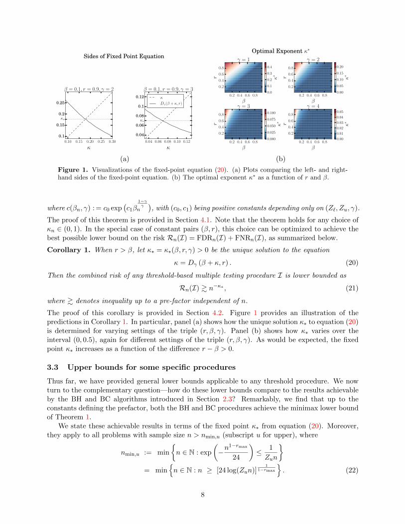
Figure 1. Visualizations of the fixed-point equation (20). (a) Plots comparing the left- and right-hand sides of the fixed-point equation. (b) The optimal exponent κ∗ as a function of r and β.

where c(βn, γ) : = c0 exp(c1β

1−γγ

n

), with (c0, c1) being positive constants depending only on (Z`, Zu, γ).

The proof of this theorem is provided in Section 4.1. Note that the theorem holds for any choice ofκn ∈ (0, 1). In the special case of constant pairs (β, r), this choice can be optimized to achieve thebest possible lower bound on the risk Rn(I) = FDRn(I) + FNRn(I), as summarized below.

Corollary 1. When r > β, let κ∗ = κ∗(β, r, γ) > 0 be the unique solution to the equation

κ = Dγ (β + κ, r) . (20)

Then the combined risk of any threshold-based multiple testing procedure I is lower bounded as

Rn(I) & n−κ∗ , (21)

where & denotes inequality up to a pre-factor independent of n.

The proof of this corollary is provided in Section 4.2. Figure 1 provides an illustration of thepredictions in Corollary 1. In particular, panel (a) shows how the unique solution κ∗ to equation (20)is determined for varying settings of the triple (r, β, γ). Panel (b) shows how κ∗ varies over theinterval (0, 0.5), again for different settings of the triple (r, β, γ). As would be expected, the fixedpoint κ∗ increases as a function of the difference r − β > 0.

3.3 Upper bounds for some specific procedures

Thus far, we have provided general lower bounds applicable to any threshold procedure. We nowturn to the complementary question—how do these lower bounds compare to the results achievableby the BH and BC algorithms introduced in Section 2.3? Remarkably, we find that up to theconstants defining the prefactor, both the BH and BC procedures achieve the minimax lower boundof Theorem 1.

We state these achievable results in terms of the fixed point κ∗ from equation (20). Moreover,they apply to all problems with sample size n > nmin,u (subscript u for upper), where

nmin,u := min

{n ∈ N : exp

(−n

1−rmax

24

)≤ 1

Zun

}= min

{n ∈ N : n ≥ [24 log(Zun)]

11−rmax

}. (22)

8

In order to state our results cleanly, let us introduce the constants

cBH :=Zu

36Z`, cBC :=

Zu48Z`

, and ζ := max{

6Z`,1

6Z`

}, (23)

and require in particular that rn ≥ rmin (κn (cAqn)) for algorithm A ∈ {BH,BC}. Note that cA < 1since Z` ≥ Zu by definition, and that the introduction of cA into the argument of rmin only changesthe minimum allowed value of rn by a conceptually negligible amount of O

(1

logn

).

Lastly, we note that BC requires an additional mild condition that the number of non-nullsn1−βn is large relative to the target FDR qn = n−κn (otherwise, in some sense, the problem is toohard if there are too few non-nulls and a very strict target FDR). Specifically, we need that bothquantities cannot simultaneously be too small, formalized by the assumption:

∃nmin,BC such that for all n ≥ nmin,BC we have3cBC

4· qn

log 1qn

· n1−βn ≥ 1. (24)

We note that when rn = r and βn = β are constants, this decay condition is satisfied by qn = n−κ∗ .Our second main theorem delivers an optimality result for the BH and BC procedures, showing

that under some regularity conditions, their performance achieves the lower bounds in Theorem 1up to constant factors.

Theorem 2. Consider the βn-sparse γ-tail generalized Gaussians testing problem with target FDRlevel qn upper bounded as in condition (16).

(a) Guarantee for BH procedure: Given a signal strength rn ≥ rmin(κn(cBHqn)) and sample sizen > nmin,u as in condition (22), the BH procedure satisfies the bounds

FDRn ≤ qn and FNRn ≤2ζ2β

1−γγ

n

BH

Zu· n−Dγ(βn+κn,rn), where ζBH := ζ

cBH. (25)

(b) Guarantee for BC procedure: Given a signal strength rn ≥ rmin(κn(cBCqn)) and sample sizen > max{nmin,BC, nmin,u} as in condition (24), the BC procedure satisfies the bounds

FDRn ≤ qn and FNRn ≤2ζ2β

1−γγ

n

BC

Zu· n−Dγ(βn+κn,rn) + qn, where ζBC := ζ

cBC. (26)

The proof of the theorem can be found in Section 4.3. For constant pairs (r, β), Theorem 2can be applied with a target FDR proportional to n−κ∗ to show that both BH and BC achieve theoptimal decay of the combined FDR-FNR up to constant factors, as stated formally below.

Corollary 2. For β < r and q∗ = c∗n−κ∗ with 0 < c∗ ≤ min

{124 ,

16Z`

}, the BH and BC procedures

with target FDR q∗ satisfy

Rn . n−κ∗ . (27)

To help visualize the result of Corollary 2, Figure 2 displays the results of some simulations of theBH procedure that show correspondence between its performance and the theoretically predictedrate of n−κ∗ . Despite the optimality, Figures 1 and 2 paint a fairly dark picture from a practicalpoint of view: while asymptotic consistency can be achieved when r > β, the convergence of therisk to zero can be extremely slow, exhibiting nonparametric rates far slower than n−1/2. Figure 2

9

0 50000 100000 150000 200000 250000

n

0.2

0.3

0.4

0.5

0.6

0.7C

ombi

ned

Ris

kActual (β = 0.6, r = 0.75)Predicted (β = 0.6, r = 0.75)Actual (β = 0.6, r = 0.825)Predicted (β = 0.6, r = 0.825)Actual (β = 0.6, r = 0.9)Predicted (β = 0.6, r = 0.9)

(a) γ = 1

0 50000 100000 150000 200000 250000

n

0.5

0.6

0.7

0.8

0.9

1.0

Com

bine

dR

isk

Actual (β = 0.6, r = 0.75)Predicted (β = 0.6, r = 0.75)Actual (β = 0.6, r = 0.825)Predicted (β = 0.6, r = 0.825)Actual (β = 0.6, r = 0.9)Predicted (β = 0.6, r = 0.9)

(b) γ = 2

Figure 2. Results of simulations comparing the predicted combined risk with the actualexperimentally-observed risk for the BH procedure. Agreement is good across the board and im-proves as the gap (r − β) increases. We believe the latter phenomenon arises because the samplingerror is a smaller fraction of the risk as the separation increases.

shows in particular that the decay to zero may be barely evident even for sample sizes as large asn = 250, 000, even with comparatively strong signals.

The nonparametric nature may arise because the dimensionality of the decision space increaseslinearly with sample size, and asymptotically, the upside of having increasing data seems to justovercome the downside of having to make an increasing number of decisions. However, non-asymptotically, one cannot hope to drive both FDR and FNR to zero at any practical samplesize in this general setting, at least when the mean signal lies below the maximum of the nulls (i.e.,rn < 1).

Regime of linear sparsity: We turn to the regime of linear sparsity—that is, when the numberof signals scales as π1n for some scalar π1 ∈ (0, 1). Recalling that we have parameterized the number

of signals as n1−βn , some algebra leads to βn =log 1

π1logn , so both Theorem 1 and Theorem 2 predict

an upper and lower bound on the risk of the form

c0 exp(c1

[log n

log 1π1

] γ−1γ )· n−κ∗ . (28)

Note that here we overload the exponent κ∗ to the case when it is nonconstant. In order tointerpret this result, observe that if rn = r is constant, then κ∗ = r

2γ − o(1), so the rate is n−r/2γ

upto subpolynomial factors in n. On the other hand, if rn = 1

logγ−1/2γ n

is at the extreme lower limit

permitted by the lower bound (ii) in (14b), then it is not hard to see that κ∗ ≈ log− γ−1/2

γ n, which

ensures that nκ∗ � exp(

logγ−1γ n

), so that the risk (28) still approaches zero asymptotically, albeit

subpolynomially in n.

4 Proofs

We now turn to the proofs of our main results, namely Theorems 1 and 2, along with Corollary 1.

10

4.1 Proof of Theorem 1

The main idea of the proof is to reduce the problem of lower bounding the FNRn of threshold-basedprocedures that use random, data-dependent thresholds Tn, to the easier problem of lower boundingthe FNRn of threshold-based procedures that use a deterministic, data-independent threshold tn.We refer to the latter class of procedures as fixed threshold procedures, and we parameterize them bytheir target FDR qn = n−κn . Concretely, we define the critical threshold, derived from the criticalregime boundary rmin from equation (15), by

τmin(κn) : =(γrmin

(κn)

log n)1/γ ≡ τmin(qn) : =

(γrmin

(log(1/qn)

log n

)log n

)1/γ

. (29)

Here and throughout the proof, we express τmin and rmin as functions of qn rather than κn; thisformulation turns out to make certain calculations in the proof simpler to express.

From data-dependent threshold to fixed threshold: Our first step is to reduce the analysisfrom data-dependent to fixed threshold procedures. In particular, consider a threshold procedure,using a possibly random threshold Tn, that satisfies the FDR uppper bound FDRn(Tn) ≤ qn. Weclaim that the FNR of any such procedure must be lower bounded as

E[FNPn(Tn)] ≥ FNRn

(τmin

(4qn))

16. (30)

This lower bound is crucial, as it reduces the study of random threshold procedures (LHS) to studyof fixed threshold procedures (RHS). In order to establish the claim (30), define the events

E1 : ={Tn ≥ τmin

(4qn)}, and E2 : =

{FNPn

(τmin

(4qn))≥ FNRn

(τmin

(4qn))

2

}.

The following lemma guarantees that both of these events have a non-vanishing probability:

Lemma 1. For any threshold Tn such that FDRn(Tn) ≤ qn, we have

P[E1](a)

≥ 3/8, and P[E2](b)

≥ 3/4. (31a)

The proof of this lemma can be found in Appendix A. Using this result, we now complete the proofof claim (30). Define the event

E : =

{FNPn(Tn) ≥ FNRn

(τmin(4qn)

)2

}.

The monotonicity of the function t 7→ FNPn(t) ensures that the inclusion E ⊇ E1 ∩ E2 must hold.Consequently, we have

P[E ] ≥ P[E1 ∩ E2] ≥ P[E2]− P[Ec1](i)

≥ 3

4− 5

8= 1/8,

where step (i) follows by applying the probability bounds from Lemma 1.Finally, by Markov’s inequality, we have

FNRn(Tn) = E[FNPn(Tn)] ≥ P[E ]FNRn

(τmin(4qn)

)2

≥ FNRn

(τmin(4qn)

)16

,

which establishes the claim (30).Our next step is to lower bound the FNR for choices of the threshold t ≥ τmin(qn):

11

Lemma 2. For any t ≥ τmin(qn), we have

FNRn(t) ≥

ζ2β1−γγ

n

Z`· n−Dγ(βn+κn,r) if r > rmin

(κn(qn)

),

12 otherwise,

(32)

where ζ was previously defined (23).

The proof of this lemma can be found in Appendix B. Armed with Lemma 2 and the lowerbound (30), we can now complete the proof of Theorem 1. We split the argument into two cases:

Case 1: First, suppose that r ≤ rmin(κn(4qn)). In this case, we have

FNRn(Tn)(i)

≥ FNRn

(τmin

(4qn))

16

(ii)

≥ 1

32,

where step (i) follows from the lower bound (30), and step (ii) follows by lower bounding the FNRby 1/2, as is guaranteed by Lemma 2 in the regime r ≤ rmin(κn(4qn)).

Case 2: Otherwise, we may assume that r > rmin(4qn). In this case, we have

FNRn(Tn)(i)

≥ FNRn

(τmin

(4qn))

16

(ii)

≥(4ζ)2β 1−γ

γn

Z`· n−Dγ(βn+κn,r).

Here step (i) follows from the lower bound (30), whereas step (ii) follows from applying Lemma 2in the regime r > rmin(κn(4qn)). With some further algebra, we find that

FNRn(Tn) ≥ 1

Z`exp

(2 log

(4ζ)· β

1−γγ

n

)n−Dγ(β+κn,r) = c0 exp

(c1β

1−γγ

n

)n−Dγ(β+κn,r),

where c0 : = 1Z`

and c1 : = 2 log(4ζ). Note that since Z` > 0 and ζ ≥ 1, both of the constants c0

and c1 are positive, as claimed in the theorem statement.

4.2 Proof of Corollary 1

We now turn the proof of Corollary 1. Although it can be proved from the statement of Theorem 1,we instead prove it more directly, as this allows us to reuse parts of the proof of Lemma 2, therebysaving some additional messy calculations.

First, we verify that there is indeed a unique solution κ∗ to the fixed point equation (20). Define

the function as g(κ) : = Dγ (β + κ, r)1/γ −κ1/γ . Clearly the solutions to (20) are the roots of g. Wewould like to argue that any such root must occur in [0, r−β) and that in fact g has a unique rootin this interval. For the first claim, note that g(r − β) = −(r − β)1/γ < 0. On the other hand, wehave

g′(κ) =

−1γ

[(β + κ)

− γ−1γ + κ

− γ−1γ

]if 0 ≤ κ < r − β,

1γ

[(β + κ)

− γ−1γ − κ−

γ−1γ

]if κ > r − β.

It is immediately clear that g′(κ) < 0 for 0 ≤ κ < r − β and, since β + κ > κ, we may also deducethat g′(κ) < 0 for κ > r − β, so g is decreasing on its domain. Therefore, g(κ) < g(r − β) < 0 for

12

all κ > r − β.3 We conclude that any root of g must occur on [0, r − β). To finish the argument,note that g(0) > 0 > g(r − β), so that g does indeed have a root on [0, r − β).

Turning now to the proof of the lower bound (21), let I be an arbitrary threshold-based multipletesting procedure. We may assume without loss of generality that

FDRn(I) ≤ min{n−κ∗ ,

1

24

}≤ c(β, γ)n−κ∗ , (33)

where the quantity c(β, γ) ≥ 1 was defined in the statement of Theorem 1 (otherwise, the claimedlower bound (21) follows immediately).

Applying the second part of Lemma 2 and defining c = 4c(β, γ) , we conclude that

FNRn

(Tn)≥ FNRn

(τmin

(cn−κ∗

))16

≥(cζ)2β 1−γ

γ

Z`· n−Dγ(β+κ∗,r)

=

(cζ)2β 1−γ

γ

Z`· n−κ∗

= c′n−κ∗ .

4.3 Proof of Theorem 2

We now aim to show that the Benjamini-Hochberg (BH) and Barber-Candes (BC) algorithmsachieve the minimax rate (19) when rn > rmin(κn(cAqn)), where A ∈ {BH, BC} and cA is thealgorithm-dependent constant defined in (23). The proof strategy for both algorithms is essentiallythe same. Given a target FDR rate qn, we apply each algorithm qn as the target FDR level and provethat the resulting threshold satisfies tA ≤ τmin(cAqn) with high probability. The known propertiesof the algorithms guarantee the required FDR bounds [as studied by the authors of 2, 13, 3], whilethe following converse to Lemma 2 provides the requisite upper bounds on the FNR.

Lemma 3. If rn > rmin

(cqn)

and t ≤ τmin(cqn) for some c > 0, then we have

FNRn

(t)≤(

max{c, 1/c

}· ζ)2β 1−γ

γn

Zu· n−Dγ(βn+κn,r),

where constant ζ is defined in (23).

4.3.1 Achievability result for the BH procedure

In this section, we prove that BH achieves the lower bound whenever rn > rmin

(cBHqn

). Specifically,

we prove the claim (25) stated in Theorem 2.As described in the previous section, the key step is to compare tBH, the random threshold set

by BH with target FDR of qn, to the critical value τmin,BH := τmin(cBHqn). To this end, we arguethat

P(tBH > τmin,BH

)≤ exp

(− n1−rmax

24

). (34)

3Note that we have suppressed the issue of non-differentiability of g at κ = r− β. We may do so because it is left-and right-differentiable at this point, and we argue separately for the intervals [0, r − β) and [r − β, ∞).

13

We begin by showing how to derive the upper bound (25) from the probability bound (34).Note that since BH is a valid FDR control procedure, we necessarily have FDRn(tBH) ≤ qn. Tobound the FNR, first let E = {tBH ≤ τmin,BH} and let FNRn(· | E) and FNRn(· | Ec) denote theFNRn conditional on the event and its complement, respectively. In this notation, the bound (34),together with Lemma 3, implies that

FNRn(tBH) ≤ P(E)· FNRn

(τmin,BH | E

)+ P

(Ec)

≤ FNRn

(τmin,BH

)+ P

(Ec)

≤ FNRn

(τmin,BH

)+ exp

(− n1−rmax

24

)≤ ζ2β

1−γγ

n

BH

Zu· n−Dγ(βn+κn,rn) + exp

(− n1−rmax

24

)≤ 2ζ2β

1−γγ

n

BH

Zu· n−Dγ(βn+κn,rn),

where the final step uses the definition (22) of nmin,u, and the fact that 1Zun≤ ζ

2β

1−γγ

nBHZu·n−Dγ(βn+κn,rn),

which is easily verified by noting that ζ2β1−γγ

n

BH ≥ 1 and Dγ (βn + κn, rn) ≤ 1.

We now prove the bound (34) with an argument using p-values and survival functions that par-allels that of Arias-Castro and Chen [2] but sidesteps CDF asymptotics. We study the relationshipbetween the population survival function Ψ and the empirical survival function Ψ, defined by

Ψ(t)

=(1− 1

nβn

)· Ψ0

(t)

+1

nβn· Ψ1

(t), (35)

where Ψ0

(t)

=1

n− n1−βn∑i∈H0

1(Xi ≥ t

)and Ψ1

(t)

=1

n1−βn

∑i/∈H0

1(Xi ≥ t

).

Now, sort the observations in decreasing order, so that X(1) ≥ X(2) ≥ · · · ≥ X(n), and define p-values

p(i) = Ψ(X(i)

)and Ψ

(X(i)

)=i

n, (36)

so that p(1) ≤ p(2) ≤ · · · ≤ p(n) are in increasing order. Then, we may characterize the indicesrejected by BH as those satisfying Xi ≥ X(iBH), where

iBH = max{

1 ≤ i ≤ n : Ψ(X(i)

)≤ qnΨ

(X(i)

) }. (37)

Moving tBH within(X(iBH+1), X(iBH)

]if necessary, we may therefore assume Ψ(tBH) = qnΨ(t)

whenever t < tBH, and combining this knowledge with (35), we obtain the chain of inclusions

Ec = {tBH ≤ τmin,BH} ⊃{

Ψ(τmin,BH

)≤ qnΨ

(τmin,BH

)}⊃{

Ψ(τmin,BH

)≤ qnnβn· Wn

n1−βn

}=: E , (38)

where Wn =∑

i/∈H01(Xi ≥ τmin,BH

)∼ Bin

(Ψ(τmin,BH − µn

), n1−βn

).

14

We now argue that Ψ(τmin,BH

)≤ qn

4nβn, so that P (E) ≥ P

(Wn >

n1−βn4

). For this, observe that

by the definition of rmin in (15) and the upper tail bound (5), we have

log Ψ(τmin,BH

)≤ −rmin (cBHqn) log n+ log

1

Zu

≤ −βn log n+ log(cBHqn)− log1

6Z`+ log

1

Zu

= −βn log n+ log qn + log6cBHZ`Zu

= logqn

6nβn< log

qn4nβn

.

We conclude

P (tBH > τmin,BH) ≤ 1− P(E)≤ 1− P

(Wn >

n1−βn

4

)= P

(Wn ≤

n1−βn

4

).

Finally, by a Bernstein bound, we find

P(Wn ≤

n1−βn

4

)≤ P

(Wn ≤

E [Wn]

2

)≤ exp

(− E [Wn]

12

)≤ exp

(− n1−βn

24

)≤ exp

(− n1−rmax

24

),

where we have used the fact that τmin,BH ≤ µn to conclude that Ψ (τmin,BH − µn) ≥ 12 and therefore

E[Wn] ≥ n1−βn2 . We have therefore established the required claim (34), concluding the proof of

optimality of the BH procedure.

4.3.2 Achievability result for the BC procedure

Our overall strategy for analyzing BC procedure resembles the one we used for the BH procedure. Aswith our analysis of the BH procedure, we define τmin,BC := τmin(cBCqn) and derive the bound (25)by controlling the algorithm’s threshold as

P (tBC > τmin,BC) ≤ qn + exp(− n1−rmax

24

). (39)

Since the proof of equation (26) from the bound (39) is essentially identical to the correspondingderivation for the BH procedure, we omit it. We now prove the bound (39) by an argumentsomewhat different than that used in analyzing the BH procedure. Define the integers

N+

(t)

=

n∑i=1

1(Xi ≥ t

)and N−

(t)

=

n∑i=1

1(Xi ≤ −t

).

Then, the definition of the BC procedure gives

tBC = inf{t ∈ R :

1 +N−(t)

1 ∨N+(t)≤ qn

}.

15

To prove (39), it therefore suffices to show that

P

(1 +N−(τmin,BC)

1 ∨N+(τmin,BC)> qn

)≤ qn + exp

(− n1−rmax

24

). (40)

We prove the bound (40) in two parts:

P(1 ∨N+(τmin,BC) <

n1−βn

4

)≤ exp

(− n1−rmax

24

), (41a)

P

(1 +N−(τmin,BC) > qn ·

n1−βn

4

)≤ qn. (41b)

These bounds are a straightforward consequence of elementary Bernstein bounds, and together theyimply the claim (40). We explain them below.

The lower bound (41a) follows because 1 ∨N+(τmin,BC) ≥ N+(τmin,BC) and N+(τmin,BC) is thesum of two binomial random variables, corresponding to nulls and signals, respectively, and thelatter has a Ψ

(τmin,BC−µ

)≥ 1

2 probability of success. More precisely, we may write N+ (τmin,BC) =

Nnull+ +N signal

+ , with

Nnull+ ∼ Bin

(Ψ (τmin,BC) , n− n1−βn

)and N signal

+ ∼ Bin(

Ψ (τmin,BC − µn) , n1−βn),

implying N+ (τmin,BC) ≥ N signal+ , whence

E[N+(τmin,BC)

]≥ E

[N signal

+

]= n1−βn ·Ψ

(τmin,BC − µn

)≥ n1−βn

2,

where we have used the fact that τmin,BC ≤ µn. With this bound in hand, a Bernstein bound yields

P(N+(τmin,BC) <

n1−βn

4

)≤ P

(N+(τmin,BC) ≤ E [N+(τmin,BC)]

2

)≤ exp

(− n1−βn

24

)≤ exp

(− n1−rmax

24

),

as required to prove equation (41a). The proof of equation (41b) follows a similar pattern. Here,we note that N−(τmin,BC) is a sum of two binomial random variables, with a total of n trials, suchthat—using the definition (15) of rmin and the upper bound on the tail (5)—each one has probabilityof success upper bounded by 1−Ψ

(− τmin,BC

)≤ 6Z`

Zu· cBCqnn

−βn = 18 · qnn−βn . Formally, we may

write N−(τmin,BC) = Nnull− +N signal

− , with

Nnull− ∼ Bin

(1−Ψ (−τmin,BC) , n− n1−βn

)and N signal

− ∼ Bin(

1−Ψ (−τmin,BC − µ) , n1−βn).

Since 1−Ψ (−τmin,BC − µ) ≤ 1−Ψ (−τmin,BC), we deduce

E[N−(τmin,BC)

]≤[1−Ψ (−τmin,BC)

]· n ≤ qn

2· n

1−βn

4.

On the other hand, using the lower bound in (5), we find 1−Ψ(− τmin,BC

)≥ 6cBCqnn

−βn . Usingthe additional fact that n− n1−βn ≥ n

2 by (14a), we may conclude that

E[N−(τmin,BC)

]≥ E

[Nnull−]

=(n− n1−βn

)·[1−Ψ

(− τmin,BC

)]≥ n

2· 6cBCqnn

−βn

≥ 3cBCqnn1−βn .

16

By a Bernstein bound, it follows that

P

(N−(τmin,BC) ≥ qn ·

n1−βn

4

)≤ P

(N−(τmin,BC) ≥ 2E

[N−(τmin,BC)

])

≤ exp

(− E

[N−(τmin,BC)

]4

)≤ exp

(− 3cBC

4· qnn1−βn

)≤ qn,

where we have invoked the decay condition (24) for the last step.

4.4 Proof of Corollary 2

The corollary is a nearly immediate consequence of Theorem 2. We will prove it for both algorithmssimultaneously. Observe that

rmin(κn(cAq∗)) = β + κ∗ +log 1

6c∗cAZ`

log n. (42)

Suppose for now that the decay condition (24) holds for q∗ and some choice of nmin,BC. Then,using (42) and the fact that r > β + κ∗, we may choose n′min ≥ nmin,BC large enough so thatr > rmin(κn(cAq∗)) for all n ≥ n′min and A ∈ {BH, BC}. From Theorem 2, we conclude that thereexists a constant c′ such that both algorithms satisfy

n ≥ n′min =⇒ Rn ≤ c′n−κ∗ .

By replacing c′ by c = max {c′, (n′min)κ∗} (and recalling Rn ≤ 1 always), we obtain Rn ≤ cn−κ∗

for all n ≥ 1, obtaining the claimed result.In order to check the decay condition (24), note that, as κ∗ ≤ r − β ≤ 1 − β, we have for

sufficiently large n that

qn

log 1qn

=n−κ∗

κ∗ log n≥ 4

3cBC· n−(1−β),

which completes the proof.

5 Discussion

Despite considerable interest in multiple testing with false discovery rate (FDR) control, therehas been relatively little understanding of the non-asymptotic trade-off between controlling FDRand the analogous measure of power known as the false non-discovery rate (FNR). In this paper,we explored this issue in the context of the sparse generalized Gaussians model, and derived thefirst non-asymptotic lower bounds on the sum of FDR and FNR. We complemented these lowerbounds by establishing the non-asymptotic minimaxity of both the Benjamini-Hochberg (BH) andBarber-Candes (BC) procedures for FDR control. The theoretical predictions are validated insimple simulations, and our results recover recent asymptotic results [2] as special cases. Ourwork introduces a simple proof strategy based on reduction to deterministic and data-obliviousprocedures. We suspect this core idea may apply to other multiple testing settings: in particular,

17

since our arguments do not depend on CDF asymptotics in the way that many classical analyses ofboth global null testing and FDR control procedures do, we hope they will be possible to adapt forother problems described below.

As mentioned after the statement of Theorem 2, the practical implications of our results aresomewhat pessimistic. Even for rather simple problems having r−β of constant order, the resultingrate at which the risk tends to zero can be far slower than n−1/2. (Indeed, it seems like such aparametric rate is only achievable when γ = 1, rn → 1, βn → 0.) Hence, in practice, one mustcarefully consider whether good FDR or good FNR is more important, as achieving both may notbe possible unless most of the signals to be identified are rather large.

Future work

A large part of the multiple testing literature focuses on the development of valid FDR control pro-cedures that can gain power or precision by explicitly using prior knowledge such as null-proportionadaptivity [25, 26], groups or partitions of hypotheses [14, 19], prior or penalty weights [4, 16],or other forms of structure [22, 24], and it would be of great interest to extend our techniquesto such structured settings. It is also important to handle the cases of positive or arbitrary de-pendence [5, 6, 24], hence this is another natural direction in which to extend our work. (Suchextensions were explored by [17, 21, 18] for the higher criticism statistic for the detection problem.)Lastly, all of the discussed literature is in the offline setting, and it could be of interest to developtight lower and upper bounds for online FDR procedures [12, 20].

A general proof technique for establishing non-asymptotic lower bounds in multiple testing re-mains an important direction for future work. As our arguments are based on analytical calculations,they are sensitive to the particular observation model under consideration. It would be desirable tobuild on our approach to identify the key properties of multiple testing problems that make themdifficult or easy, and establish lower bounds in terms of these properties. We hope our work willhelp lay the foundation for progress in understanding the limits of multiple testing more generally.

Acknowledgements

This work was partially supported by Office of Naval Research Grant DOD-ONR-N00014, Air ForceOffice of Scientific Research Grant AFOSR-FA9550-14-1-0016, and Office of Naval Research grantW911NF-16-1-0368NSF. In addition, MR was supported by an NSF Graduate Research Fellowshipand a Fannie and John Hertz Foundation Google Fellowship.

A Proof of Lemma 1

This appendix is devoted to the proof of Lemma 1, which was involved in the proof of Theorem 1.Our proof makes use of the following auxiliary lemma:

Lemma 4. For qn ∈ (0, 1/24), we have

P[FDPn

(t)≥ 8qn for all t ∈ [0, τmin(4qn)]

]≥ 1

2. (43)

We return to prove this claim in Appendix A.1. For the moment, we take it as given and completethe proof of Lemma 1.

18

Control of E1: Let us now prove the first bound in Lemma 1, namely that P[E1] ≥ 38 where

E1 : ={Tn ≥ τmin(4qn)

}. So as to simplify notation, let us define the event

D : ={

FDPn(t)≥ 8qn for all t ∈ [0, τmin(4qn)]

}. (44a)

Now observe that

P[Tn ≥ τmin

(4qn)]≥ P

[Tn ≥ τmin

(4qn)

and D]

= P[D]− P[Tn ≤ τmin

(4qn)

and D]. (44b)

Now by the definition (44a) of the event D, we have the inclusion{Tn ≤ τmin

(4qn)

and D}⊆{

FDPn(Tn) ≥ 8qn

}.

Combining with our earlier bound (44b), we see that

P[Tn ≥ τmin

(4qn)]≥ P[D]− P

[FDPn(Tn) ≥ 8qn

].

It remains to control the two probabilities on the right-hand side of this bound. Applying Lemma 4guarantees that P[D] ≥ 1

2 . On the other hand, by Markov’s inequality, the assumed lower bound

FDRn

(Tn)≤ qn implies that P

[FDPn

(Tn)≥ 8qn

]≤ 1

8 . Putting together the pieces, we conclude

that

P[E1] = P[Tn ≥ τmin

(4qn)]≥ 1

2− 1

8=

3

8,

as claimed.

Control of E2: Let us now prove the lower bound P[E2] ≥ 3/4. We split our analysis into twocases.

Case 1: First, suppose that rn > rmin. In this case, we can write

FNPn(t) =Fn(t)

n1−βn, where Fn

(t)∼ Bin

(1−Ψ

(t− µ

), n1−βn

).

Since rmin > βn, we have

µ− τmin ≥(γ log n

)1/γ[r1/γn − β1/γn

]≥(γ log n

)1/γ · (rn − βn)1/γ ,from which it follows that

E[Fn] = 1−Ψ(t− µ

)≥ nβn−rn

Z`. (45)

Now by applying the Bernstein bound to the binomial random variable Fn, we have

1− P[E2] = P[Fn ≤

E[Fn]

2

]≤ exp

(− E[Fn]

12

)(i)

≤ exp(− n1−rn

12Z`

)(ii)

≤ exp(− n1−rmax

12Z`

), (46)

where step (i) follows from the lower bound (45), and step (ii) follows since rn < rmax by assumption.

19

Case 2: Otherwise, we may assume that rn ∈(βn, r

−1n

). In this regime, we have the lower bound

τmin − µ ≥ 0, so that the binomial random variable Fn stochastically dominates a second binomialdistributed as Fn ∼ Bin

(12 , n

1−βn). By this stochastic domination condition, it follows that

1− P[E2]≤ P

[Fn ≤

n1−βn

4

]≤ P

[Fn ≤

E[Fn

]2

].

By applying the Bernstein bound to Fn, we find that

1− P[E2]≤ exp

(− n1−βn

24

)≤ exp

(− n1−rmax

24

), (47)

where the final step follows since rmax > βn.

Putting together the two bounds (46) and (47), we conclude that P[E2] ≥ 34 for all sample sizes n

large enough to ensure that

max{

exp(− n1−rmax

24Z`

), exp

(− n1−rmax

24

)}≤ 1

4, (48)

as was claimed. Note that condition (48) is identical to condition (17), so that our definition ofnmin guarantees that (48) is satisfied. This completes the proof.

A.1 Proof of Lemma 4

It remains to prove our auxiliary result stated in Lemma 4. For notational economy, let τ = τmin(s)and let β = βn. The FDP at a threshold t can be expressed in terms of two binomial randomvariables

Ln(t)

=∑i∈H0

1(Xi ≥ t

)and Wn

(t)

=∑i/∈H0

1(Xi ≥ t

)≤ n1−β.

Here Ln(t) and Wn(t) correspond (respectively) to the number of nulls, and the number of signalsthat exceed the threshold t. In terms of these two binomial random variables, we have the expression

FDPn(t) =Ln(t)

Ln(t) +Wn(t)≥ Ln(t)

Ln(t) + n1−β.

Note that the inequality here follows by replacing Wn(t) by the potentially very loose upper boundn1−β; doing so allows us to reduce the problem of bounding the FDP to control of Ln(t) uniformlyfor t ∈ [0, τ ]. By definition of Ln(t), we have the lower bound

Ln(t)

Ln(t) + n1−β≥ Ln(τ)

Ln(τ) + n1−βfor all t ∈ [0, τ ].

Moreover, observe that

3s

1 + 3s≥ 12

5s ≥ 2s for all s ∈ (0, 1/6).

Combining these bounds, we find that

P[FDPn(t) ≥ 2s for all t ∈ [0, τ ]

]≥ P

[ Ln(τ)

Ln(τ)

+ n1−β≥ 3s

1 + 3s

]= P

[Ln(τ) ≥ 3sn1−β

].

20

Consequently, the remainder of our proof is devoted to proving that

P[Ln(τ) ≥ 3sn1−β

]≥ 1/2. (49)

We split our analysis into two cases:

Case 1: First, suppose that qn ≥ 2 log 43n1−β In this case, we have

α : = Ψ(τ)≥ 6s

nβ>

16 log 4

n. (50)

A simple calculation based on this inequality yields

αn− 3sn1−β ≥ αn

2≥√(

4 log 4)α(1− α

)n : = aσ, (51)

where a =√

4 log 4 and σ =√α(1− α

)n. Notice that σ2 = Var [Ln(τ)].

We now apply the Bernstein inequality to Ln(τ) to obtain

P(Ln ≤ 3sn1−β

)≤ P

(Ln ≤ π1n− aσ

)≤ 2 · exp

(− a2σ2

2[σ2 + aσ

])≤ 2 · exp

(− a2

2(1 + a

σ

)).≤ exp

(− a2

4

)=

1

4,

where we have used the fact that a < σ. We conclude that

P(Ln ≥ 3sn1−β

)≥ 1

2,

as desired.

Case 2: Otherwise, we may assume that qn <2 log 43n1−β . The definition of τ implies that

α ≥ 24

nand 3sn1−β ≤ 8 log 4.

It follows that E[Ln(τ)] ≥ 24. On the other hand, given that 8 log 4 < 12, it suffices to prove that

P[Ln(τ) ≤ 12

]≤ 1

2.

This is straightforward, however, since Bernstein’s inequality gives

P[Ln(τ) ≤ 12

]= P

[Ln(τ) ≤ E[Ln(τ)]

2

]≤ exp

(− 24

12

)= e−2

<1

2,

which completes the proof.

21

B Proof of Lemmas 2 and 3

This appendix is devoted to the proofs of Lemmas 2 and 3. We combine the proofs, since these twolemmas provide lower and upper bounds, respectively, on the because they are matching lower andupper bounds, respectively, on the FNR for a fixed threshold procedure, and their proofs involveextremely similar calculations.

So as to simplify notation, we make use of the convenient shorthands let τ = τmin(qn), β = βn,

and µ = µn throughout the proof. Recall that the FNP can be written as the ratio FNPn(t) = Fn(t)n1−β ,

where

Fn(t) =∑i/∈H0

1(Xi ≤ t

)∼ Bin

(1−Ψ

(t− µ

), n1−β

)(52)

is a binomial random variable. We split the remainder of the analysis into two cases.

Case 1: First, suppose that τ ≥ µ. In this case, we only seek to prove a lower bound. For this,observe that Ψ (τ − µ) ≤ Ψ (0) = 1

2 , so 1−Ψ (τ − µ) ≥ 12 . Thus,

FDRn (τ) =E [Fn]

n1−β= 1−Ψ (τ − µ) ≥ 1

2,

as claimed.

Case 2: Otherwise, we may assume that µ > τ . Recall the parameterization (13) of µ in terms ofr, the definition (15) of rmin, and the definition (18) of the Dγ distance. In terms of these quantities,we have

µ− τ =(γ log n

)1/γ {r1/γ − rmin(κn)

}1/γ={γDγ

(rmin(κn), r

)log n

}1/γ

=[γDγ

(β + κn +

log 16Z`

log n, r)

log n]1/γ

,

which shows how the quantity Dγ determines the rate. In order to complete the proof, we need toshow that the additional order of 1

logn term inside Dγ can be removed.

More precisely, it suffices to establish the sandwich relation

ζ2β1−γγ

Zu· n−Dγ(β+κn,r) ≥ 1−Ψ

(τ − µ

)≥ ζ2β

1−γγ

Z`· n−Dγ(β+κn,r),

where ζ = max{

6Z`,1

6Z`

}as in (23). But now note that

τ − µ =(γ log n

)1/γ[(rmin

)1/γ − r] = −[γDγ (rmin, r) log n

]1/γ,

allowing us to deduce that

1

Zu· n−Dγ(rmin,r) ≥ 1−Ψ

(τ − µ

)≥ 1

Z`· nDγ(rmin,r),

22

so we need only show

∣∣Dγ (β + κn, r)−Dγ (rmin, r)∣∣ ≤ β

1−γγ log ζ

log n.

To prove this, we let

r : = min(β + κn, rmin

)and note that by (16), we must have r ∈ [β, r]. Under this definition, we consider the functionf(x) = Dγ (r + x, r). A simple calculation shows that for x ≥ 0, we have

f ′(x) =

−(r + x

) 1−γγ Dγ (r + x, r)

γ−1γ if r + x ≤ r,(

r + x) 1−γ

γ Dγ (r + x, r)γ−1γ o.w.

We observe that we only need to allow 0 ≤ x ≤ max(β + κn, rmin

)− r =: R − r, so in particular,

we will always have r + x ≤ R ≤ 2. This, together with the lower bound r ≥ β, yields

sup0≤x≤R−r

∣∣f ′(x)∣∣ ≤ 2β

1−γγ .

Applying this result, we find∣∣Dγ (β + κn, r)−Dγ (rmin, r)∣∣ =

∣∣Dγ

(R, r

)−Dγ (r, r)

∣∣≤ 2β

1−γγ ·

(R− r

)= 2β

1−γγ · log ζ

log n.

If we now consider q′n = cqn, we can recover the more refined statements in Lemmas 2 and 3,simply by noting that the same reasoning as above shows

∣∣Dγ (β + κn, r)−Dγ

(β + κ′n, r

) ∣∣ ≤ 2β1−γγ ·

∣∣ log c∣∣

log n,

concluding the argument.

References

[1] F. Abramovich, Y. Benjamini, D. Donoho, and I.M. Johnstone. Adapting to unknown sparsityby controlling the false discovery rate. Annals of Statistics, 34(2):584–653, 2006.

[2] E. Arias-Castro and S. Chen. Distribution-free multiple testing. arXiv preprintarXiv:1604.07520, 2016.

[3] Y. Benjamini and Y. Hochberg. Controlling the false discovery rate: A practical and powerfulapproach to multiple testing. Journal of the Royal Statistical Society: Series B (StatisticalMethodology), 57(1):289–300, 1995.

[4] Y. Benjamini and Y. Hochberg. Multiple hypotheses testing with weights. ScandinavianJournal of Statistics, 24(3):407–418, 1997.

23

[5] Y. Benjamini and D. Yekutieli. The control of the false discovery rate in multiple testing underdependency. Annals of Statistics, 29(4):1165–1188, 2001.

[6] G. Blanchard and E. Roquain. Two simple sufficient conditions for FDR control. ElectronicJournal of Statistics, 2:963–992, 2008.

[7] M. Bogdan, A. Chakrabarti, F. Frommlet, and J.K. Ghosh. Asymptotic Bayes-optimality undersparsity of some multiple testing procedures. Annals of Statistics, 39(3):1551–1579, 2011.

[8] Z. Chi. On the performance of FDR control: Constraints and a partial solution. Annals ofStatistics, 35(4):1409–1431, 2007.

[9] D. Donoho and J. Jin. Higher criticism for detecting sparse heterogeneous mixtures. Annalsof Statistics, 32(3):962–994, 2004.

[10] D. Donoho and J. Jin. Asymptotic minimaxity of false discovery rate thresholding for sparseexponential data. Annals of Statistics, 34(6):2980–3018, 2006.

[11] D. Donoho and J. Jin. Higher criticism for large-scale inference, especially for rare and weakeffects. Statistical Science, 30(1):1–25, 2015.

[12] D.P. Foster and R.A. Stine. α-investing: A procedure for sequential control of expected falsediscoveries. Journal of the Royal Statistical Society: Series B (Statistical Methodology), 70(2):429–444, 2008.

[13] R. Foygel Barber and E.J. Candes. Controlling the false discovery rate via knockoffs. Annalsof Statistics, 43(5):2055–2085, 2015.

[14] R. Foygel Barber and A. Ramdas. The p-filter: Multi-layer FDR control for grouped hypotheses.Journal of the Royal Statistical Society: Series B (Statistical Methodology), 2016.

[15] C.R. Genovese and L. Wasserman. Operating characteristics and extensions of the false discov-ery rate procedure. Journal of the Royal Statistical Society: Series B (Statistical Methodology),64(3):499–517, 2002.

[16] C.R. Genovese, K. Roeder, and L. Wasserman. False discovery control with p-value weighting.Biometrika, 93(3):509–524, 2006.

[17] P. Hall and J. Jin. Properties of higher criticism under strong dependence. Annals of Statistics,36(1):381–402, 2008.

[18] P. Hall and J. Jin. Innovated higher criticism for detecting sparse signals in correlated noise.Annals of Statistics, 38(3):1686–1732, 2010.

[19] J. Hu, H. Zhao, and H. Zhou. False discovery rate control with groups. Journal of the AmericanStatistical Association, 105(491):1215–1227, 2010.

[20] A. Javanmard and A. Montanari. On online control of false discovery rate. arXiv preprintarXiv:1502.06197, 2015.

[21] J. Jin and T. Ke. Rare and weak effects in large-scale inference: Methods and phase diagrams.arXiv preprint arXiv:1410.4578, 2014.

24

[22] A. Li and R. Foygel Barber. Multiple testing with the structure adaptive Benjamini-Hochbergalgorithm. arXiv preprint arXiv:1606.07926, 2016.

[23] Pierre Neuvial and Etienne Roquain. On false discovery rate thresholding for classificationunder sparsity. Annals of Statistics, 40(5):2572–2600, 2012.

[24] A. Ramdas, R. Foygel Barber, M.J. Wainwright, and M.I. Jordan. A unified treatment ofmultiple testing with prior knowledge. arXiv preprint arXiv:1703.06222, 2017.

[25] J. Storey. A direct approach to false discovery rates. Journal of the Royal Statistical Society:Series B (Statistical Methodology), 64(3):479–498, 2002.

[26] J. Storey, J. Taylor, and D. Siegmund. Strong control, conservative point estimation andsimultaneous conservative consistency of false discovery rates: A unified approach. Journal ofthe Royal Statistical Society: Series B (Statistical Methodology), 66(1):187–205, 2004.

[27] J.W. Tukey. The Problem of Multiple Comparisons: Introduction and Parts A, B, and C.Princeton University, 1953.

25