OPTIMAL PRODUCT LINE DESIGN WHEN CONSUMERSEXHIBIT CHOICE SET DEPENDENT PREFERENCES

A.YESIM ORHUN

Preliminary, Comments Welcome

September 2005Haas School of Business, University of California at Berkeley

Abstract. Research in Marketing and Psychology has shown that a product’srelative standing in a choice set can influence its utility. Consequently, theindependence of irrelevant alternatives assumption is frequently violated. Thispaper incorporates this robust empirical regularity into a model of product linedesign in order to investigate how a firm’s product positioning and portfoliostrategies change if the potential customers exhibit such preferences. To thisend, a general reference-dependent utility framework that incorporates lossaversion is employed, where the reference point is endogenous to the choiceset.

The optimal product line width and the product positions differ from thoseof the standard model. Specifically, the extended model yields three sharp pre-dictions in regards to market outcomes when consumer preferences are choiceset dependent:

Compression Effect : Compared to the strategy recommendations of stan-dard economic models, the optimal product positions are such that the rangesof the attributes are compressed towards the reference point. Given a productwidth, the extent of compression is increased by the degree of loss aversion.

Pooling Effect : A further implication of the compression effect is the poolingeffect where the firm offers only a single product to serve multiple segments ofcustomers even though it is costless to introduce a product. This finding runscounter to the standard model predictions.

Augmentation Effect : The firm manages its product line such that it mayintroduce or delete a product simply to augment utilities of other products.The “augmenting” product portfolio improves the perceived reference point ofkey consumer segments, a market phenomenon that could not be accountedfor by the standard model.

The results show that it is important for the firm to quantify the degree ofchoice set dependency of preferences in formulating the optimal product linestrategy.

1

2 A.YESIM ORHUN

1. Introduction

Product line design is one of the most important marketing-mix decisions. In

order to decide on the number and positioning of products in its product line, a

firm must understand the manner in which consumers evaluate and choose prod-

ucts. Existing methods frequently adopt utility specifications that assume that

consumer preferences are independent of the choice set. However there is ample

evidence that customers often violate this assumption of independence. Some of

the evidence include extremeness aversion, asymmetric dominance, asymmetric

advantage, detraction, and enhancement effects (Huber, Payne and Puto (1982),

Simonson(1989), Simonson and Tversky(1992)). It is important to capture these

observed violations to the standard utility framework in order to develop optimal

product line strategies for a firm which faces vertically differentiated consumer

segments.

To this end, this paper develops a general utility model that is flexible enough

to allow for various patterns of choice set dependent preferences. Choice set de-

pendency refers to the violation of the principle that the preference structure is

independent of the choice set. This dependence is captured by a model that is

based on the concept of reference dependence and loss aversion, where reference

levels are determined by the choice set the consumer is presented with. The pro-

posed utility specification extends the loss aversion concept to multi dimensions,

includes the consumption utility as well as comparative utility. This comparative

utility captures the importance of the relative standing of a product with respect

to others in the choice set. It depends on the valuation of the departures of

attribute levels of a product from the reference point where the reference point

is endogenously determined by the products in the choice set. This formulation

allows us to separately study the effects of the sensitivity to losses and the sensi-

tivity to gains on the product line strategies of the firm. The presented framework

is psychologically richer than the standard framework and it reduces to the latter

when choice set dependency is not present.

Having specified a utility framework that captures the co-movement of prefer-

ences and the choice set, this paper proceeds to study how the product line design

3

changes as a result. If consumer preferences are choice set dependent, a firm of-

fering a menu of products should not only consider the substitution between

alternatives and the selection motives, but also take into account how each prod-

uct’s demand will be affected by its relative standing among the other products.

As a result of this consideration, the firm responds with different strategies. Thus

the proposed model is used to derive new implications for optimal firm strategies

in regards to the product line design.

Conditional on the number of products, the firm introduces distortions in qual-

ity provisions, due to the influence of each product’s position on the demand of

others in the product line. Thus, contrary to the standard models, the consumer

segment with the highest value for quality with respect to price, may receive less

than the quality provided if this segment were the only one in the market. On

the other hand, the lowest-end consumer segment will receive a higher quality

provision compared to the standard model. Therefore, the range of the quality

offered will be narrower, as the end quality provisions are compressed towards

the reference point, a result labelled as the “compression effect” in this paper.

The extent of this compression depends on the degree of loss aversion. In general,

the degree of quality distortion for any segment is proportional to the influence

of the segment’s product on the relative standing of other products.

Since the existence as well as the positioning of a product affects the relative

standing of other products, the product line length also is a tool for profit man-

agement. The firm may trim the product line to serve all consumers with the

same product, if the increase in profits due to separation is outweighed by the

loss in profits due to loss aversion induced by comparisons. This result is called

the “pooling effect”. The intuition behind the pooling effect is that by offering

several products the firm may make consumers worse off since this introduces

perceived losses in comparative evaluations. Consequently, the firm is better off

by serving some or all consumers with just one product instead of going after

the extra rents that could be extracted by separation. This finding provides an

explanation to why some firms target the low-end and the high-end segments

with the same product, even when the standard framework would predict that

the firm leaves money on the table by not separating the high-end consumers. By

4 A.YESIM ORHUN

targeting the high-end consumers with a different offering, the firm may lower its

profits because the product offering meant for high-end customers will decrease

low-end consumers’ utility for any given product. Therefore the firm may pool

the types even if segmentation is costless.

Another finding that cannot be predicted by the standard model is that the

firm may change the number of products carried and the choice of segments

served, simply to increase profits from key segments in the market by influencing

their perceived relative standing. The “augmentation effect” refers to this finding

where the firm may manage the reference point by the addition or the deletion of

products, and thus enhances the utility that the key segments derive from their

offerings. Although these trimming or extension strategies may not be profitable

on their own, they increase the total profits derived from the product line. For

example, the firm may find it profitable to stop serving a segment, if the absence

of the product for that segment moves the reference point in a favorable fashion

for the profits extracted from other key segments. Alternatively, the firm may add

a product to manage the reference point. In such a case, the additional product

serves a consumer segment that would not have been served otherwise, since that

segment would not be profitable on its own. This phenomenon, while occurring

frequently in the real world, cannot be explained by the standard framework.

In sum, this paper proposes a general utility framework that is descriptive

of the consumer behavior which has been documented to violate the standard

framework. Based on this general framework, new strategy recommendations

are derived for firms facing vertically differentiated consumer segments which

cannot be identified a priori. To arrive at these managerial recommendations,

the paper builds on the findings and strengths of research across different fields.

Consequently, it fills the gap between our understanding of the actual behavior of

consumers and the strategy recommendations regarding the product line design.

The rest of the paper is organized as follows. Section 2 provides an overview of

the related literature and presents the utility framework that extends the standard

model to account for choice set dependency. Section 3 analyzes the outcomes in

the marketplace with two vertically differentiated consumer segments and Section

4 discusses the extensions of the model such as increasing the number of segments

5

and studying the effect of excess utility from gains as well as loss aversion. Section

5 concludes.

2. Previous Literature and a Choice Set Dependent Utility

Specification

Robust findings of local context effects provide evidence for the violation of

the assumption of independence of preferences and the choice set. Some of these

context effects have been documented by Simonson and Tversky (1992), Simonson

(1989), Huber, Payne and Puto (1982), to name a few. I would refer the interested

reader to Drolet, Simonson and Tversky (2000) for a more complete overview of

how choice set influences choice. It is clear from the findings of the literature that

consumers may violate the Independence of Irrelevant Alternatives assumption

at the individual level and that their preferences may depend on the choice set.

Simonson and Tversky (1992) show that the intermediate options fare better

than extreme options and label this effect as “extremeness aversion”. When

people exhibit extremeness aversion toward both attributes, this effect is called

the “compromise effect”. We can represent these findings, in Figure 1, where

alternative L will fare better if presented in the choice set of {K,L,M} than

in the choice set of {L,M,N}. The opposite will be true for alternative M. In

the same article, Simonson and Tversky also demonstrate “enhancement” and

“detraction” effects. Enhancement effect labels the observation that option F in

Figure 2 does better when presented with both A and B, than when presented

with either A or B. Detraction effect labels the observation that option G does

worse when presented with both A and B than when presented with either of

the two. Moreoever, Huber, Payne and Puto (1982) and Simonson (1989) have

demonstrated “asymmetric dominance” and “asymmetric advantage” effects, as

depicted in Figure 3. The addition of alternative D to the choice set of {A,B},increases the share of B compared to A, and the addition of alternative E to the

choice set {A,B} increases the relative share of A.

Just as Drolet, Simonson and Tversky (2000) put, this empirical evidence sug-

gests that preferences “travel” with the choice set. This paper aim to propose

a utility framework that captures this observation and systematically explains

6 A.YESIM ORHUN

the directional deviations of these findings from the standard utility framework.

Previous work by Tversky and Simonson (1993) and Kivetz, Netzer and Srini-

vasan (2004a, 2004b) aimed at capturing observed deviations with different util-

ity models. The former work employs a tournament model to capture context

dependency. The proposed model pairwise compares each alternative to other

alternatives in the choice set and weighs losses more than gains. The latter work

empirically tests alternative theories that may explain compromise effect and also

discusses how proposed models can explain other context effects. This research

finds empirical evidence that modeling the local choice context leads to better

predictions and fit compared to that of the traditional models. The authors find

support for models that use a single reference point over tournament models.

Their proposed model rests on loss aversion and reference dependence, where

the reference point for each attribute is the mid-point of the observed range of

that attribute. Wernerfelt (1995) explains the existence of the compromise effect

with a setup where consumers do not know their preferences, except for their

place in the distribution and can infer their types from what the firm offers, who

is assumed to know the distribution of tastes. However Prelec, Wernerfelt and

Zettelmeyer (1997) show that the compromise effect can only be explained in part

with the proposed theory. Although many behavioral theories are proposed for

the context effects documented, the common concept underlying all these mod-

els is that consumers make comparative evaluations and care about the relative

standing of a product.

This paper proposes a utility framework which incorporates the evidence on

the local context effects with the use of reference dependent preferences. The

proposed model uses a novel reference point formation, where the reference point

travels with the choice set. This is how the effects of the choice set on the prefer-

ence structure is captured. This framework is a psychologically richer version of

the standard utility framework and reduces back to it when there is no reference

dependence.

This formulation extends the reference dependent utility model of Kahneman

and Tversky (1991) to include both the consumption utility and gain-loss utility,

as in Koszegi and Rabin (2005). This approach allows the researcher to compare

7

the relative importance of two sources of utility, while extending the standard

framework. It rests on the observation that both the departures from the refer-

ence point matter for utility, as well as the levels of consumption. Furthermore

this approach allows us to study the effects of the different aspects of compar-

ative evaluations separately, namely loss sensitivity and gain sensitivity. This

feature is essential in identifying the way in which the gain sensitivity and the

loss sensitivity influence firm’s strategies in different ways.

The total valuation for a given product is assumed to be separately additive

over all attributes of the product as well as the utility types. Let the products in

a choice set be indexed by j = {1, 2, ..., J} and the attributes of the products be

indexed by k = {1, 2, ..., K}. Then the individual i’s utility for product j can be

expressed as

uij =K∑

k=1

vi(xjk) +K∑

k=1

fk(vi(xjk)− vi(rk))

where vi(xjk) is the choice set independent consumption utility and fk(vi(xjk)−vi(rk)) is the comparative utility. In this formulation, if y > y′ > 0, then fk(y) +

fk(−y) < fk(y′)+fk(−y′), which captures the main intuition of loss aversion that

the same change in the attribute levels matter more when the consumer perceives

to be in losses in that attribute than when she perceives to be in gains in that

attribute. Around the reference point fk(·) has a local kink,limx→0 f ′k(−|x|)limx→0 f ′k(|x|) ≡

δk > 1. Fixing δk, the importance of the comparative utility is increasing in

limx→0 f ′k(|x|).Using the following function is sufficient to capture the effects of gain and loss

sensitivity 1,

fk(v(xjk)− v(rk)) =

{λk · [v(xjk)− v(rk)] if xjk < rk

γk · [v(xjk)− v(rk)] if xjk ≥ rk

1When taking this model to data one may want to allow and test for diminishing sensitivity inthe comparative utility.

8 A.YESIM ORHUN

where λk ≥ γk ≥ 0 ∀k and rk = g(x1k, x2k, ..., xJk). In order for this model to

capture choice set dependency, the reference point for each attribute is designed

to be a function of the attribute levels of products in the choice set. A reason-

able assumption on g(·) is that the reference point is a weighted average of the

attribute levels in the choice set2, rk =∑J

j=1 ρjxjk where∑J

j=1 ρj = 1. This

formulation is general enough to allow for any reference point within the convex

hull of the observed attributes.

In sum, both the absolute level of consumption as well as the relative standing

of a product matter for the overall utility of a product. This approach enables

us to measure how important comparative evaluations are with respect to the

utility from consumption alone. Moreover it allows us to study different aspects

of comparative evaluations. The loss parameter, λk, captures the dis-utility of

being in the losses compared to the reference point. When the losses are zero,

the total utility equals the consumption utility. To capture the intuition of loss

aversion, this parameter alone is sufficient. The gain parameter, γk, on the other

hand, captures the increase in utility of being in the gains compared to the

reference point. For example, in the price dimension, this reflects the increased

utility due to knowing that one paid less than one expected, in other words,

some sort of a “deal effect”. When both the gain and the loss parameters are

considered, the ratio of these parameters capture the degree to which the gains

are weighed less than the losses in the comparative evaluations.

We can illustrate how the changes in the comparative evaluations affect the

indifference curves, given a reference point. Consider, as an example, a consumer

with linear indifference curves over two attributes labelled as x1 and x2 in the

illustration in the next page. In this example, the indifference curves of a con-

sumer under the standard model are labelled with the letter A. The indifference

curves labelled as B represent the same utility level as their A counterparts in

a model which accounts for the consumer’s sensitivity towards losses. At the

reference point and in the domain of gains in both attributes, the indifference

2The reference point can alternatively be formed such that the linear combination is not takenover attributes but the valuation of attributes. The two approaches are equivalent when utilityis linear in attributes.

9

curves coincide. However, the level of utility decreases in regions of loss due to

the introduction of loss aversion. Also, since the attribute sensitivities increase

in the domain of losses, the slope of the indifference curves change across regions.

In the domain of losses in both attributes, the indifference curves reflect the

overall decreased utility. If the loss sensitivities are the same for both attributes,

the indifference curve in this domain is parallel to the standard one. However this

does not need to be the case, as depicted by the dashed line, where the impact of

losses in attribute x is lower than the impact of losses in attribute y. In regions

where the consumer perceives to be in losses only in one of the attributes, the

consumer is more sensitive towards that attribute. The change of slopes across

regions of gain and loss reflect this phenomenon. When the consumer is sensitive

towards losses, the level of utility of the consumer is lower than or equal to that in

the standard case, resulting in the indifference curves to be enveloped by standard

indifference curves.

The effect of gains in the comparative utility is twofold. The attribute sen-

sitivities in regions of gain increase as gain sensitivities increase. Also the level

of utility increases for any given product, except those that are perceived to be

in losses in both dimensions. Therefore the slopes of indifference curves deviate

less from those in the standard model, and the utility levels are more than those

in the standard model in the region of gains in both dimensions. The second

10 A.YESIM ORHUN

illustration depicts an example of how the indifference curves may look under

a model that considers gains as well as losses in the comparative utility. The

indifference curves labelled as C illustrate how the utility changes compared to

the standard model (A) or compared to a model with only loss sensitivity (B).

These examples demonstrated how the indifference curves change across regions

of gain and loss and how the intensity of this change depended on the difference in

the sensitivities towards losses versus gains. These examples depicted indifference

curves where the reference point was given exogenously, and the choice set did

not affect the reference point. However, in the proposed model, the way in which

choice set dependency gets factored into the model is through the reference point

formation. Although the preferences are stable within the choice set, changes in

the choice set may lead to preference reversals. We can show how changing the

choice set leads to unstable preferences with a simplified example, demonstrated

in the following page. Consider two choice sets where the position of the products

denoted with A and B are the same across choice sets, but the third product is

shifted along the vertical dimension. To the extent that the third alternative in

the choice set, H, affects the reference point3, the reference point is shifted along

3Assume for simplicity of demonstration that only the presented choice set affects the referencepoint.

11

the vertical dimension as well. As a result of this change in the third alternative,

ranking of alternatives A and B change.

This is due to the fact that losses loom larger than gains. Therefore the increase

in losses (in the vertical dimension) for alternative B decreases its utility more

than the same amount of decrease in gains does for alternative A. Due to changes

in the reference point, across choice sets, indifference curves may cross and thus

preference reversals may occur.

Therefore the preferences will travel with the choice set, to the extent that

changes in the choice set reflect on the reference point. This approach translates

12 A.YESIM ORHUN

the classical utility model into a psychologically richer one without changing the

core formulation, so if the consumers do not exhibit any context dependence in

their preferences, the model reduces back to the standard model.

The model captures the empirical regularities labelled as extremeness aver-

sion, asymmetric dominance and advantage effects, enhancement and detraction

effects. It also explains the changes in the shares of two extreme options, as a

result of local changes in the middle option, which does not change the range

of the attributes. Please see the Appendix for more details on how this utility

framework captures the mentioned local context effects.

3. Optimal Menu Design with Vertically Differentiated

Consumers

Profit maximizing firms will take into account the fact that the alternatives

in the menu which are not targeted to a particular consumer are still going to

influence her valuation of the alternative that is targeted to her, since it will define

the relative standing of that alternative. This will result in a rich interaction of

substitution, selection and spill-over effects. The following model incorporates

these considerations, and offers an explanation to some product line strategies

that are not in line with the current models.

Consider the case where a firm faces different consumer segments with differ-

ent attribute sensitivities, however does not have information about a specific

consumer’s sensitivity. The firm can offer a menu of products, which leads the

consumers to self-select into buying one of them. This problem has been stud-

ied extensively under the standard utility framework (Mussa and Rosen, 1978,

Maskin and Riley, 1984).

Assume that the firm is offering one type of good with two attributes, which

can be quality and price. Assume there are two segments of consumers; segment

h has a higher valuation of quality over price compared to segment l. The firm

wants to choose a menu of products that will elicit the types of consumers and

extract the highest possible surplus.

13

Let ql, qh be the qualities that types l and h respectively buy, and pl, ph be the

prices they pay for these alternatives. Then the firm’s objective is to maximize

Π =∑

i∈L,H

αi(pi − c(qi))

where αi is the proportion of type i ∈ L, H consumers in the population. The

marginal cost function c(·) equals zero when q = 0 and is assumed to be twice

differentiable and strictly convex. Firm chooses the most profitable (pl, ql) and

(ph, qh) it will offer if it finds it optimal to serve both segments. The utility of

each type i = l, h is

Ui(q, p|qr, pr) = θiq − p + fq(θiq − θiqr) + fp(pr − p)

where

fq(θiq − θiqr) =

{0 if q ≥ qr

−λqθi(qr − q) if q < qr

and

fp(p− pr) =

{0 if p < pr

−λp(p− pr) if p > pr

The reference point for an attribute is a linear combination of all the level of

attributes in the choice set4.

pr = ηlpl + ηhph

where ηl + ηh = 1. The reference quality is formed similarly

qr = µlql + µhqh

where µl + µh = 1.

4This is a uni-reference model, where the reference point is formed by some weighting of theattribute levels observed in the choice set. The model can be extended to allow for differ-ent reference point formations for the evaluation of each alternative, if such an extension isbehaviorally warranted.

14 A.YESIM ORHUN

If the consumers can be ordered in their relative valuations of quality versus

money5, then the optimal quality provisions are increasing in these valuations.

Thus in equilibrium, ql < qr < qh and pl < pr < ph.

The consumers’ outside utility is normalized to zero. If a consumer buys a

product, it should be the case that the product provides at least zero utility.

This is known as the Individual Rationality (IR) constraint. Also in equilibrium

the firm wants each consumer to find the product intended for his/her type the

most desirable in the product line. This is known as the Incentive Compatibility

(IC) constraint. The firm maximizes its profits subject to these constraints. The

IR constraint for the low type and the IC constraint for the high type are binding6.

The Individual Rationality (IR) constraint for the low type is

Ul(ql, pl|qr, pr) ≥ 0

⇒ θl[ql − λq(qr − ql)]− pl ≥ 0

Note that the utility of the low type consumer is reduced for any given quality

level due to the dis-utility she incurs from being in losses in quality.

The Incentive Compatibility (IC) constraint for the high type is

Uh(qh, ph|qr, pr) ≥ Uh(ql, pl|qr, pr)

⇒ θhqh − ph − λp(ph − pr) ≥ θh[ql − λq(qr − ql)]− pl

which reflects decreased utility of consuming the high end product due to losses

in the price dimension. On the other hand, the utility of consuming the low

end product decreases in the loss aversion in quality. Therefore as the disutility

associated with losses in the quality dimension increases, the IC constraint is

easier to satisfy and the firm can charge a higher price to the high type for the

same quality offering at the high end.

The prices that can be charged to the type l and type h consumers are de-

termined by the IC constraint binding for the high type and the IR constraint

5For this ordering to be preserved across the parameter space, the choice set dependency ofpreferences should not overwhelm type differences, Particularly, I assume that θh/θl > (1 +λpηl)(1 + λqµh)6Please see appendix for why these sets of constraint are the only ones that bind.

15

binding for the low type. Equilibrium prices are

pl = θl[ql − λq(qr − ql)]

and

ph =1

1 + λpηl

[θhqh − [θh − (1 + λpηl)θl](ql − λq(qr − ql))]

When we introduce disutility due to losses to the standard model, the price

that can be charged for the low end product is decreasing in the loss parameter for

the quality dimension. Due to the disutility that the high type consumer would

incur if she consumed the lower end product, the price that can be charged for

the high end product is increasing in the loss aversion in quality. In other words,

it is easier to convince the high type not to pretend, without having to give a high

information rent7. Therefore, compared to the standard model, the IC constraint

becomes easier to satisfy, at given quality levels, because the high type would

hate losses in quality more than the low type does. Consequently, loss sensitivity

in quality decreases information rent.

One important feature of this model is that the attribute sensitivities are not

only type but also consumption instance specific. For example, the high type

consumer cares more about marginal changes in the quality when she deviates

and consumes the low end product, but her valuation of quality does not change

for the product that is targeted to her. Therefore this model makes it easier for

the firm to separate the high type without leaving too much rent on the table.

This is an important difference between decreasing the differentiation between

two types in the standard model and a model with loss aversion. The underlying

preference structure of types shift with respect to their relative offers. A firm that

has a naive model of context-independent preferences, and observes the relative

valuation of types, will leave too much rent on the table, assuming that the high

type will have the same high valuation if it deviated to the low type’s product.

However the firm can use the existence of loss aversion to its advantage if it has

the right model in mind.

7The information rent of the high type, (θh − θl)ql − λq(θh − θl)[qr − ql], decreases in the lossaversion for quality.

16 A.YESIM ORHUN

Losses in prices, λp, can effectively be seen to make the high type consumers

more price sensitive, thus reducing the price that can be charged for any given

quality level.

The total profits of the firm decrease with relative losses in the price dimension.

Given how the prices and profits change with the model parameters, we can now

examine the optimal quality provisions.

The firm’s problem is to maximize profits with respect to quality levels for high

and low types,

maxql,qh

Π =∑

i∈L,H

αi(pi − c(qi))

s.t.IR = 0, IC = 0

Proposition 3.1. The sensitivity for losses results in an increase in the optimal

quality provision of the low type, due to the increased quality sensitivity of the

low type and the negative influence of its price on the profits extracted from the

high type.

Proof. We can characterize the optimal quality provision to type l implicitly as

c′(ql) =(1 + µhλq)(θl − αhθh

1+λpηl)

αl

Since the marginal cost function is convex in q, we can see that the quality

provision for the low type will be higher than the standard case and will increase

in both loss aversion parameters. �

Distortion at the bottom in this model is a result of several considerations on

the firm’s side. The firm decreases the quality provision to the low type in order

to minimize the information rent left to the high type. This makes deviation less

attractive for the high type, therefore the high type is willing to pay more for his

quality provision. However this effect is dimmed by the loss aversion in prices,

which increases the effective price sensitivity of the high type, and decreases the

price that can be charged to this segment. As a result of this effective decrease

in the marginal valuation of the high type, the level of distortion at the bottom

is decreased. Moreover, the firm realizes that the utility of the high type can be

17

increased by increasing the reference price. To the extent that the price of the

low type’s quality provision affects the reference price, the firm finds it profitable

to increase the low type’s quality provision.

Furthermore, to the extent that the low type cares about losses in quality, the

quality sensitivity of the low type increases. Therefore, the firm faces an upward

pressure in the quality provision for the low type.

Proposition 3.2. The sensitivity for losses results in a decrease in the optimal

quality provision of the high type, due to the increased price sensitivity of the high

type and the negative influence of its quality provision on the profits extracted

from the low type.

Proof. We can describe the quality provision to the high type as

c′(qh) =

αhθh

1+λpηl− µhλq(θl − αhθh

1+λpηl)

αh

�

Loss aversion in quality reduces qh since the firm realizes that, to the extent

that the high type’s quality provision affects the reference quality, it increases the

utility of the low type consumer by decreasing the quality provision to the high

type. As long as the firm finds it profitable to serve both segments in equilibrium,

this effect will overwhelm the reduction of the information rent. Therefore, an

increase in the loss aversion in quality will decrease the quality provision to the

high type. Furthermore, the loss aversion in price reduces qh since the effective

price sensitivity of the high type is increased by loss aversion.

Combining the results on quality provisions for both types, we see that the

inclusion of loss sensitivity compresses the range of quality provided in the mar-

ketplace. Loss aversion in each dimension contributes to the result independently.

The “compression effect” is based on two main forces. One is the fact that con-

sumers become more sensitive for the attribute they perceive to be in losses. The

other is the realization of the firm that the positioning of each product has an

influence on the relative standing of the other product, and therefore its valua-

tion. Thus the firm finds it profitable to move the attribute levels towards the

18 A.YESIM ORHUN

reference point. The compression effect gets more pronounced with the degree

of loss aversion compared to the consumption utility. When the loss aversion is

very important, the distance between the offerings may collapse.

Proposition 3.3. If the loss aversion in quality is large enough, then the firm

will find it profitable to pool the two types.

Proof.

c′(qh)− c′(ql) =αh(

θh

1+λpηl− θl)− µhλq(θl − αhθh

1+λpηl)

αlαh

this difference will be positive only if

µhλq <αh(θh − θl(1 + λpηl))

θl(1 + λpηl)− αhθh

Since c(·) is convex, this shows that qh > ql only when the above condition holds.

If the loss aversion is big enough, quality provision to both types will be equal.

Therefore in equilibrium, the two types may be pooled, even when separation is

costless. �

In the standard framework, the quality provision of the high type is strictly

bigger than that of the low type, which is a result of the monopolist finding

serving both types of consumers with different products always more profitable

than serving all types with one product. However the loss aversion decreases the

differentiation of two products. When the loss aversion in quality is large enough,

µhλq > αh(θh−θl(1+λpηl))

θl(1+λpηl)−αhθh, the firm may find it profitable to serve all segments only

with one product. Although under the standard model for all parameters f ′(qh)−f ′(ql) > 0, it may not be the case under this model due to loss aversion. Unlike

the standard framework, loss aversion in quality might result in this “pooling

effect” in equilibrium. This is due to the fact that serving the high type with

a separate product creates a negative influence on the utility of the low type.

Existence of price loss aversion makes this even more severe, by decreasing the

revenues extracted from the high type in the case of separation. Therefore the

19

firm may find that the decrease in the rents that can be extracted overwhelms

the profits from separation.

Now let us examine the decision of whether to serve both types of consumers

in equilibrium, or only to serve the high type consumers. The existence of loss

aversion in prices which makes the high type more price sensitive and less prof-

itable may suggest that the firm will serve the low type in more circumstances.

However this intuition is wrong, since the influence of the low type’s price offer

to the high type’s utility disappears when the low type is not served. This result

highlights why this model is different than a model that simply changes the rela-

tive valuations of segments. If in equilibrium, the low type is not served, the firm

can charge a much higher price to the high type, not only because there would

be no need for information rent, but also because the high type would not be in

losses in the price.

Proposition 3.4. When the firm separates the low and high type, its profit de-

creases in the loss parameters, and is lower than its counterpart in the standard

model.

Proof. Loss aversion in both attributes decrease profits when the firm finds it

profitable that both types consume positive amounts in equilibrium.

dΠ

dλp

= − θhαhηl

(1 + λpηl)2[qh − ql + λq(qr − ql)]

dΠ

dλq

= −(qr − ql)(θl −αhθh

1 + λpη)

When the firm serves only the high type, its profit is

Πh = αh(θhq∗h − c(q∗h))

where q∗h is the socially optimal quality provision, s.t. c′(q∗2) = θh

c. This is the

same profit as in the standard case, due to the fact that choice set dependency

disappears when there is just one product offered.

20 A.YESIM ORHUN

When the firm serves both types, its profit is

Πl,h =αh[θh

1 + λpη1

qh − (θh

1 + λpηl

− θl)(ql + λq(qr − ql)− c(qh))]

+ αl[θl(ql − λq(qr − ql))− c(ql)]

where the optimal quality provisions are as above. The firm will serve both

segments only if Πl,h > Πh.

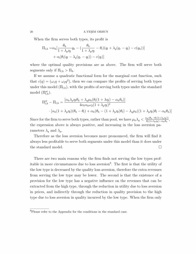
If we assume a quadratic functional form for the marginal cost function, such

that c(q) = (ω1q + ω2q2), then we can compare the profits of serving both types

under this model (Πl,h), with the profits of serving both types under the standard

model (Πstl,h).

Πstl,h − Πl,h =

[αhλpηlθh + λqµh(θl(1 + ληl)− αhθh)]

4αlαhω2(1 + λpηl)2

· [αh(1 + λpηl)(θh − θl) + αh(θh − (1 + λpηl)θl)− λqµh((1 + λpηl)θl − αhθh)]

Since for the firm to serve both types, rather than pool, we have µhλq < αh(θh−θl(1+λpηl))

θl(1+λpηl)−αhθh,

the expression above is always positive, and increasing in the loss aversion pa-

rameters λq and λp.

Therefore as the loss aversion becomes more pronounced, the firm will find it

always less profitable to serve both segments under this model than it does under

the standard model. �

There are two main reasons why the firm finds not serving the low types prof-

itable in more circumstances due to loss aversion8. The first is that the utility of

the low type is decreased by the quality loss aversion, therefore the extra revenues

from serving the low type may be lower. The second is that the existence of a

provision for the low type has a negative influence on the revenues that can be

extracted from the high type, through the reduction in utility due to loss aversion

in prices, and indirectly through the reduction in quality provision to the high

type due to loss aversion in quality incurred by the low type. When the firm only

8Please refer to the Appendix for the conditions in the standard case.

21

offers a product to the high segment, the high segment’s relative quality valua-

tion is augmented compared to the case where the firm provides also a lower end

product. This is why this type of strategy is called the “augmentation effect”.

This result demonstrates that choice set dependent preferences differ from the

standard framework in an important way. It highlights the observation that

the relevant utility functions are different under different choice scenarios for

the same type of consumers. This insight has been presented before regarding

how the firm can make more money by understanding that the preference of a

high type consumer will change if she were to deviate and consume the low end

product. The structure which leads the firm to charge more to the high type due

to increased punishment of deviation, also is the same structure that provides

incentives to stop serving the low type or to pool the two types.

A higher price sensitivity of the high type and a higher quality sensitivity of

the low type would also result in less differentiation. However this change in

the attribute sensitivities would not result in non-stable valuation rules across

alternatives and choice sets. The existence of the comparative utility results in

a preference structure that changes across regions of gain and loss. Therefore

preferences are consumption specific as well as type specific. This means that

the high type will not have the same valuation of quality when consuming the

product offered to the low type. Similarly, the consumer will not have the same

preferences if they were presented with only one option rather than a menu. The

first effect, as we discussed, leads to the firm leaving less information rent to the

high type. The second effect, may result in pooling since the existence of another

product makes both segments incur loss disutility. Similarly, this effect may also

decrease the incentives to serve the low type, since providing a positive quality

option to the low type, with a lower price, induces price loss aversion for the high

type, which would not happen with one option.

The compression effect is a result of two main forces. The first is the fact that

the consumers are more sensitive towards attributes that they perceive to be in

losses in. The second is the fact that the firm realizes the influence of each prod-

uct’s position onto other product’s evaluation and manages these comparisons in

its favor. The pooling effect, in the example with two segments, is strengthened by

22 A.YESIM ORHUN

the fact that when there is only one product in the choice set, that product is the

reference point, and therefore the choice set dependency disappears. However,

as we will see, this effect carries onto cases with more consumer segments. The

main reason behind the pooling effect is that the firm can eliminate unwanted

comparisons which increases the rents from key segments. It is a result of the firm

using the effect of the existence of products to its favor. This is one of the ways

in which the firm can manage profits by managing the reference point. Similarly,

the augmentation effect is a result of the firm’s ability to enhance the utility of

its consumers by managing the reference point through the existence of products

in the choice set. In the case with two segments, we saw that the firm may stop

serving the low type segment, since not having a lower price point makes the

high type consumers much happier about the price they are paying. Studying an

extension with more than two types will give us richer interactions of this sort.

4. Extensions

The framework with two segments of consumers demonstrates the main forces

that affects the optimal product line design. There are two important extensions

to the current model. The first is to examine how the generalization of the model

to more than two types contributes to our understanding. Second is to study the

different strategies a firm can take if its consumers also have excess utility from

perceived gains in an attribute, over and beyond the consumption utility.

4.1. Three Segments of Vertically Differentiated Consumers. The main

forces that drive the product line strategies in the two segment case extend to

cases with more consumer segments although the spill-over structure becomes

more complex. A special feature of the two segment framework is that pooling

or serving one segment less, both lead to elimination of choice set dependency,

since the choice set reduces to one option. Moreover, in the framework with two

segments, whether a product is in the loss or the gain region with respect to the

reference point is stable. However, in a framework of three segments, the product

targeted to the middle segment might be in the gain region for quality when there

is a product targeted to the low segment, but will be in the loss region for quality

23

if the firm does not serve the low segment. These differences will result in a richer

set of product positioning possibilities.

It can be seen from the optimal quality provisions in a framework with three

segments in the Appendix that when the firm serves more than one segment,

the influence of one product’s positioning onto other products’ evaluations follow

the same intuition as in the two-segment case. The firm may pool the middle

and the high type consumers, which would never be the case in the standard

model. This “pooling effect” extends from the two segment case, due to negative

influence the higher types’ quality provisions have on the lower types’ utilities.

There is also more of an incentive to pool the middle type consumers with the

low type consumer as this would increase the utility of the high type if the high

type cares about losses in the price dimension. In general, the distortions in the

quality provision to each segment is proportional to the effect of the segment’s

quality and price provision onto the reference points in these dimensions. If the

segment’s product is highly influential, the distortion will be higher. Also the

distortions increase with loss aversion parameters as before.

Studying more than two types contributes to our intuition about the results of

choice set dependency, since dropping only one type or pooling only two types

does not bring us back to the standard model. It highlights strategies of firms that

may seem unprofitable, if the choice set dependency is not taken into account,

such as carrying products solely for the purposes of perception management,

which we labelled as the “augmentation effect”.

In the previous section we’ve seen that the firm may manage choice set depen-

dent valuations by dropping the low segment. However, the following stylized

example demonstrates how the choice set dependency might in fact incentivise

the firm to serve more segments, in order to augment the utility of other seg-

ments. In particular, as this example will show, when the loss aversion in quality

is significant and the proportion of middle types is large, the firm might drop the

low type less often than it would in the standard case, if serving the low type

decreases the middle type’s losses in quality.

Assuming a quadratic cost function, we can compare the decision to stop serv-

ing the low type under the standard framework, and compare it to a specialized

24 A.YESIM ORHUN

case of this framework. We will concentrate on the effect of loss aversion in

quality. Assume that when the firm offers three products, the reference point

for quality is perceived to be below the quality provision of the middle type.

Assume that type’s quality sensitivities are such that an equal proportion of con-

sumer segments lead to the firm serving all segments if costs are zero, thus equal

proportion of consumer segments is assumed.

In the standard framework, the firm will serve the low type if K ≡ Πstl,m,h −

Πstm,h > 0, and similarly in our framework if N ≡ Πl,m,h−Πm,h > 0. Please see the

appendix for the derivation of profits when the middle type’s quality level is above

the reference point. If the firm would serve the low types in our framework in

cases where the firm would have stopped serving them in the standard framework,

we expect N > K. We find that

N −K =λq

6γ2

· ((3θl − 2θm)(θh(µm − µh)− 2θmµm+

(3θl − 2θm)(µh(1 + λqµh) + βµhµm + µm(1 + λqµm)))

+ νh(2θm − θh)[2(θh − θm)− λqνh(2θm − θh)])

where νh is the weight of the high type’s quality provision on the reference quality

when the low type buys no good in equilibrium. This expression increases in the

loss aversion parameter λq, as well as νh. The bigger the νh, the higher the losses

the middle type would be incurring if the firm did not serve the low type segment.

When the weight of the low type’s offer on the reference quality is approaching

one, this expression will always be positive.

This example shows that in cases where the profits from the low type consumers

are too small for the firm to find it profitable to serve them in the standard case,

for example due to fixed costs of introduction of a product, the firm may serve

them in our framework. The firm provides a low quality product because its

existence augments the utility of the middle type. This example of the augmen-

tation effect parallels the compromise effect findings in the empirical literature.

This can often be seen in the marketplace, as the cheapest wine induces sales

of the second cheapest, and the worst cell phone option induces the sales of the

25

next ones up. The basic reason behind such an augmentation effect is that the

firm can manage the relative standing of a product, or in other words, where the

reference point is, by the addition of another product in the menu. In the cases

where this strategy actually results in a segment’s perception to change regions

(from losses to gains), as in this example, the profits from such a move is even

more profitable. However, even in cases where the perceived distance from the

reference point is reduced in the loss domain, rather than elimination of losses,

this strategy may be useful.

For example, similar effect can be found for the positive influence the high end

product has on the middle product, due to the decreased perceived losses in price,

if not the elimination of such losses. This influence increases the quality provision

of the high type (see Appendix). When there are fixed costs to introducing

products, a firm that may not find it profitable to serve the high type in the

standard model, may do so due to its positive externalities on the middle type,

if the proportion of the middle segment is very large.

4.2. Studying Gain Sensitivity. Having studied the results of loss aversion, let

us extend the comparative utility to include utility from gains. It is an advantage

that the model can incorporate the effects of introducing loss aversion and gain

sensitivity separately, since these phenomena may occur independently. It is

an empirical question whether the gain sensitivity is large enough to change

the direction of the strategies of the firms. This section extends the strategy

recommendations of the paper in cases where the firm can profit by managing

the perceived gains of consumer segments. Since the effect of gains are smaller

than the effect of losses, in many scenarios, this inclusion may not change the

directional results in optimal quality provisions. In cases where the directional

results do not change, the magnitude of the discrepancy of the results from those

of the standard model will be decreased.

26 A.YESIM ORHUN

The utility of each type i = l, h is

Ui(q, p|qr, pr) = θiq − p + fq(θiq − θiqr) + fp(pr − p)

where

fq(θiq − θiqr) =

{γqθi(q − qr) if q ≥ qr

−λqθi(qr − q) if q < qr

and

fp(p− pr) =

{γp(pr − p) if p < pr

−λp(p− pr) if p > pr

In this setup, the Individual Rationality (IR) constraint for the low type is

Ul(ql, pl|qr, pr) ≥ 0

⇒ θl[ql − λq(qr − ql)]− pl + γp(pr − pl) ≥ 0

Note that the utility of the low type consumer is reduced for any given quality

level due to the dis-utility she incurs from being in losses in quality. On the other

hand, to the extent that being in gains in the price dimension makes consumers

happier about their purchase, the utility is enhanced.

The Incentive Compatibility (IC) constraint for the high type is

Uh(qh, ph|qr, pr) ≥ Uh(ql, pl|qr, pr)

⇒ θh[qh + γq(qh − qr)]− ph − λp(ph − pr) ≥ θh[ql − λq(qr − ql)]− pl + γp(pr − pl)

which reflects increased utility from consuming the high end product due to gains

in quality, and decreased utility due to losses in prices. Although the loss aversion

in quality makes the IC constraint easier to satisfy, the gains in price and quality

weaken this effect.

The prices that can be charged to the type l and type h consumers are

pl =[1 + λpηl + γpηh]−1{(1 + λpηl)θl[ql − λq(qr − ql)]

+ γpηh[θh(qh + γq(qh − qr))− (θh − θl)(ql − λq(qr − ql))]}

27

and

ph =[ 1 + λpηl + γpηh]−1{θh(1 + γpηh)(qh + γq(qh − qr))

− [θh − (1 + λpηl)θl + γpηh(θh − θl)](ql − λq(qr − ql))}

The inclusion of gains parameters, in both dimensions, increase the price

charged to the high type. It is straightforward that when the consumers care

a lot about being in gains in quality, the high-end product will seem more at-

tractive, and consumers will be willing to pay more for the same item. The gains

in the price dimension puts an upward pressure on the prices charged for the

high end product, to the extent that this product influences the reference price,

in order to increase the utility of the low-type consumer for any given quality

level. The net effect of gains in prices is positive on the price of the high end

product. Although the IC constraint is harder to satisfy as γp increases, this

effect is outweighed by the utility increase of the low type.

The inclusion of gain parameters affect the utility of the low type through the

gain parameter in prices. The direct effect of γp on the price that can be extracted

from the low type is positive, since it increases this segment’s utility for any given

quality-price bundle. The gain sensitivity in quality, γq, also increases the low end

price. This is an indirect effect through γp. Since the gains in quality increase

the high end product’s price, to the extend that the high price contributes to

the reference price, the reference price is increased. This increases the perceived

gains in prices for the low type consumer, thus increasing the price that can be

extracted from them. Similarly, an increase in the loss aversion in prices, λp, will

decrease the price that can be charged to the high type, which also decreases pl.

These effects only exist to the extent that γp is significant. The effect of losses

in quality has a more intricate effect on the price of the low end product. It

has a negative influence through the decreased utility due to losses in quality,

as discussed above, which makes the IR constraint harder to satisfy. However,

on the other hand, since the losses in quality makes the IC constraint easier to

satisfy for the high type, ph increases, resulting in an increase in utility for the

low type, to the extent that γp is significant. Therefore the net effect will depend

28 A.YESIM ORHUN

on the sign of the term [γpηh(θh − θl)− θl(1 + λpηl)]. As long as the loss aversion

in prices is large enough compared to the difference in types or the effect of the

high type’s product on the reference price is small enough, 1+λpηl

γpηh> θh−θl

θl, losses

in quality will decrease pl.

The total profits of the firm decrease with relative losses in the price dimension,

and increase with relative importance of gains in both dimensions.

The optimal quality provisions can be described as

c′(ql) =(1 + µhλq)θl(1 + λpηl + γpηh)− (αh + γpηh)θh(1 + λqµh + γqµl)

αl(1 + λpηl + γpηh)

c′(qh) =(αh + γpηh)θh(1 + λqµh + γqµl)− θl(µhλq)(1 + λpηl + γpηh)

αh(1 + λpηl + γpηh)

Keeping the loss parameters constant, the quality provision of the high type

increases with both gain parameters, and the quality provision of the low type

decreases with both gain parameters.

As long as (θlµhλq +αhθh)(1+λpηl +γpηh) > (αh+γpηh)θh(1+λqµh+γqµl), the

previous findings that the low type will receive more and the high type will receive

less quality than they would under the standard model and that profits will be

lower will carry through. If this condition is reversed, these observations will be

reversed. Studying the effects of comparisons in each dimension separately, we

find that this condition implies that the loss aversion parameters should be large

enough compared to the gain parameters. In a case where the only comparisons

are made on the quality dimension, the quality provisions will be compressed

towards the reference point if λq

γq> µlαhθh

µh(θl−αhθh). Similarly, in a case where only the

comparisons in the price dimension matter, the quality range will be compressed

as long as the loss to gain ratio in prices is large enough compared to the ratio of

consumer segments and the influence of their price on the reference price, λp

γp>

αlηh

αhηl. The difference between the quality provisions can be implicitly described

as

f ′(qh)− f ′(ql) =[αlαh(1 + λpηl + γpηh)]−1{(αh + γpηh)θh(1 + λqµh + γqµl)

− θl(αh + µhλq)(1 + λpηl + γpηh)}

29

Compared to a model with only the loss parameters, this difference is greater.

The firm will find it profitable to pool both types if the loss aversion in quality

is large enough. In a case where only the comparisons in quality matter, this

translates to the condition that µhλq(θl − αhθh) > αh(θh − θl) + αhθhµlγq. Due

to the gains parameter in quality dimension, this condition will be satisfied less

easily than in the case with just loss parameters. In general, the condition for

pooling is, θl(αh +µhλq)(1+λpηl +γpηh) ≥ (αh +γpηh)θh(1+λqµh +γqµl), which

is made easier by the loss aversion in the price dimension, if λp

γp> αlηh

αhηl.

An intuitive result when the gain sensitivity in the quality dimension as well as

the proportion of the high type segment is high is that the firm may keep serving

the low end segment in cases where under the standard model it would not have

found it optimal to do so.

5. Discussion and Conclusion

The goal in this paper was to fill the gap between our understanding of the

actual behavior of consumers and our optimal product line strategies. To this

end, a fully specified model of choice set dependent preferences which can accom-

modate existing evidence was suggested. The building block of the utility model

is that the consumers care about comparative utility as well as consumption util-

ity and that the comparative utility is defined with respect to a reference point

which is endogenously formed by the choice set. The focal point of the paper is

the proposal that a firm facing different segments of consumers it would like to

separate, should realize the potential to manage the utility of consumers through

the product line it offers.

The model provides insight into optimal mechanism design problems, where the

principal is offering a list of options to induce self-selection of agents, who have

choice set dependent preferences. The paper highlights new strategies provided

by this model which depart from the predictions of the standard model.

Contrary to a model which does not consider choice set dependency, it suggests

that the quality provision for the highest types will be different depending on

whether this segment is served alone or with other segments. This effect is due

to the negative influence of the high types’ product on the utility of types that

30 A.YESIM ORHUN

are in losses in quality. This distortion at the top is a novel effect. Following the

same spill-over reasoning, the quality provision to the low types will be higher as

the loss aversion parameters increase. This “compression effect” increases as the

loss aversion in choice set dependency becomes stronger.

The firms might find pooling to be profitable if the disutility from loss aver-

sion is high enough. This result is also contradictory to the standard strategy

recommendations, since pooling is never optimal under the standard model.

It also provides insight to when the choice set dependency will result in more

or less products in a product line. It finds support for carrying products whose

only purpose is to manage the relative standing of key segments’ products in a

favorable way. For the same reason, those products that have a negative influence

on the relative standing of important segments may be dropped. This “augmen-

tation effect”” underlines how the firm can increase the profits it can extract from

some segments by managing the existence of products for other segments.

The model provides evidence that choice set dependence of preferences can

lead to marketplace outcomes that are distinct and highlights the importance

and need to take such effects into account when studying demand or strategic

decisions of firms. For example, allowing for such effects will be crucial when

a firm knows the attribute sensitivities in a given choice set and would like to

predict behavior in other choice sets. The firm would leave money on the table

if it naively projects the local tradeoff in attributes to other regions of gain

and loss. The model provides a profitable tools for firms in their product line

decisions. It also demonstrates how the marketplace changes as a result of choice

set dependency on the consumers’ side.

The suggested utility framework captures local context effects, however does

not aim to model the process behind the observed consumer behavior. As long as

this framework is successful in capturing the changes in consumer choice behavior

as a result of changes in the choice set, the implications for the firm strategies

are robust to the underlying behavioral mechanisms.

It should be noted that the way in which the model introduces the sensitivity

towards losses and gains does not keep a normalization of utility levels compared

to those under the standard model. The loss aversion leads to overall lowering

31

of the utility, for example. However the interesting comparisons for the firm

concerning its profits are between two different scenarios; one where the firm

is facing consumers with choice set dependent preferences, and naively uses the

standard model to design its menu, and another where it uses the proposed model.

An example of this sort was demonstrated in the case of the firm making more

profits by realizing that the IC constraint is easier to satisfy as a result of losses

in the quality dimension. Therefore the results should be interpreted keeping this

normalization problem in mind.

Several aspect of the model fall short of an ideal formulation, since some of the

assumptions are based on intuition rather than direct evidence. These aspects

can be refined with further empirical evidence. For example, the reference point

formation is modelled as a linear combination of the alternatives in the choice

set. This formulation can be extended to take past experiences or expectations

into account. As long as the firm knows where the reference point is and how it

moves with the changes in the choice set, the reference point does not have to be

in the convex hull of the alternatives for the general results of the model to go

through.

Another assumption on the reference point formation is that the reference point

is perceived to be the same for each segment and the weights are exogenously de-

termined. If the reference point is determined by the product that sells the most,

or if it is determined by the products the consumer did not buy, this assumption

will not hold. Although the details of the model will change, the qualitative re-

sults will be similar. For example, a model that constructs the reference point by

the products a consumer did not buy (counterfactual thinking) will exaggerate

the effects. If the reference point is the product that most of the consumers buy,

then all the mentioned effects will carry through, and moreover the firm will have

more incentives to pool certain segments together in order to move the reference

point to a more favorable position. The way people construct the reference point

is an important research question. The exact strategy implications for a firm will

depend on the actual reference point formation. On the other hand, the cur-

rent specification captures the main intuitions about how the results will change

32 A.YESIM ORHUN

as context dependency is more pronounced, which was the main interest of this

paper.

Finally, the model also assumes that the sensitivity to the comparative utility

in an attribute with respect to the comparative utility in other attributes for

a given consumer, is proportional to the attribute sensitivity ratios. In other

words, a consumer that is more quality sensitive than other consumers is also

more sensitive to losses and gains in quality than other consumers. Although

this assumption follows the common intuition behind earlier work, it was not

based on direct evidence in this paper. This is another area of empirical research

that has direct implications for the assumptions of this model.

References

[1] Drolet, Aimee L., Itamar Simonson, and Amos Tversky (2000), “Indifference Curves ThatTravel with the Choice Set,” Marketing Letters, 11 (3), 199-209.

[2] Huber, Joel, John W. Payne, and Christopher P. Puto (1982), “Adding AsymmetricallyDominated Alternatives: Violations of Regularity and the Similarity Hypothesis,” Journalof Consumer Research, 9 (June), 90–98.

[3] Kivetz, Ran, Oded Netzer and V. Srinivasan (2004), “Alternative Models for Capturingthe Compromise Effect,” Journal of Marketing Research, 41 (August), 237-57.

[4] Kivetz, Ran, Oded Netzer and V. Srinivasan (2004), “Extending Compromise Effect Mod-els,” Journal of Marketing Research, 41 (August), 262-68.

[5] Koszegi, Botond and Mathhew Rabin (2005), “ A Model of Reference-Dependent Prefer-ences”, Working Paper, University of California, Berkeley.

[6] Maskin, Eric and John Riley (1984), “Monopoly with Incomplete Information,” RANDJournal of Economics, 15 (2), Summer, 171-96.

[7] Mussa, M. and S. Rosen (1978), “Monopoly and Product Quality,” Journal of EconomicTheory, 18, 301-17.

[8] Orhun, Yesim (2005), “Experimental Investigation of choice set dependency,” workingpaper, University of California, Berkeley.

[9] Prelec, Drazen, Birger Wernerfelt, and Florian Zettelmeyer (1997), “The Role of Infer-ence in Context Effects: Inferring What You Want from What Is Available,” Journal ofConsumer Research, 24 (June), 118-25.

[10] Simonson, Itamar (1989), “Choice Based on Reasons: The Case of Attraction and Com-promise Effects,” Journal of Consumer Research, 16(2), 158-74.

33

[11] Simonson, Itamar and Amos Tversky (1992), “Choice in Context: Tradeoff Contrast andExtremeness Aversion,” Journal of Marketing Research, 29(August), 281-95.

[12] Tversky, Amos and Daniel Kahneman (1991), “Loss Aversion in Riskless Choice: AReference-Dependent Model,” Quarterly Journal of Economics, 106 (November), 1039-61.

[13] Tversky, Amos and Itamar Simonson (1993), “Context Dependent Preferences,” Manage-ment Science, 39(10), 1179-89.

[14] Wernerfelt, Birger (1995), “A Rational Reconstruction of the Compromise Effect: UsingMarket Data to Infer Utilities,” Journal of Consumer Research, 21 (March), 627-33.

6. Appendix

6.1. How the proposed utility framework captures local context effects.

Compromise effect can be captured with a model that uses the average of ob-

served attributes in the choice set, which will set the reference point closer to

the intermediate option than the extreme options. Since losses loom larger than

gains, the consumer would prefer to incur very small losses (or none at all) and

very small gains around the reference point, rather than to incur a big loss and

a big gain. When extremeness aversion is exhibited only towards one attribute,

this effect is called polarization, which can be captured by allowing the loss aver-

sion parameters to be attribute specific. The way that the model captures the

extremeness aversion findings is in the same spirit of the loss aversion model

proposed by Kivetz, Netzer, and Srinivasan (2004).

Detraction and Enhancement effects can also be explained by the proposed

model. In Figure 2, F is likely to be in the gain region for both attributes

compared to the reference point generated by the choice set {A,B,F}, and G is

in the loss region (albeit small) for both attributes compared to the reference

point generated by {A,B,G}, where are A and B have losses in one attribute and

gains in another. However in binary comparisons, for example {A,F}, both A

and F have losses in one attribute and gains in another. The fact that F fares

better in {A,B,F} than in both binary comparisons suggests that the consumers

exhibit loss aversion in both attributes. The fact that detraction is observed

34 A.YESIM ORHUN

suggests that the small losses on both dimensions are causing bigger disutility

than a bigger loss and a bigger gain in either dimension, which calibrates the

model’s parameters. This effect cannot be captured with a linear comparative

utility, and rests on the degree of its concavity.

Asymmetric advantage and asymmetric dominance effects can also be captured

by this model. For example, in Figure 3, the addition of E pulls the reference point

in ”attribute y” up, and slightly decreases the reference point in ”attribute x”.

This reduces the perceived losses in ”attribute x” associated with the purchase of

A, and increases the perceived losses in ”attribute y” associated with purchasing

B. Similarly, the addition of D decreases the reference point in ”attribute y”,

which decreases B’s losses, and this decrease is more utility enhancing than the

increase in gains in the same dimension for alternative A. Therefore B’s relative

share increases.

In a recent study (Orhun, 2005), consumers demonstrated sensitivity to the

position of the intermediate option when evaluating the relative attractiveness of

the extreme options, as depicted in Figure 4. Alternative A’s relative share to

alternative B was increased when the intermediate option was either X or S, and

decreased when the intermediate option was Y or T. This finding supports the

proposed model that weights all the attributes present in a choice set, rather than

using the range to determine the reference point. As demonstrated, the proposed

utility function is flexible enough to capture the documented context effects, and

can be used for estimation of how the consumer preferences are affected by the

choice set.

6.2. IR constraint for the high type is slack. Information rent is positive.

6.3. IC constraint for the low type with respect to the high type’s

product is slack. We need to show that

θl[(1+λq)ql−λqqr]−pl+γp(pr−pl) > θl[(1+γq)qh−γqqr]−ph−λp(ph−pr)

Note that pr = ηlpl + ηhph.Therefore equivalently we need to show that

(ph − pl)(1 + γpηh + λpηl) > θl([(1 + γq)qh − γqqr]− [(1 + λq)ql − λqqr])

35

Due to IRl and IC lh,

pl =(1 + λpηl)θl[ql − λq(qr − ql)]− γpηh[θh(qh + γq(qh − qr))− (θh − θl)((1 + λq)ql − λqqr)]

1 + λpηl + γpηh

and

ph =θh(1 + γpηh)(qh + γq(qh − qr))− [θh − (1 + λpηl)θl + γpηh(θh − θl)]((1 + λq)ql − λqqr)

1 + λpηl + γpηh

We have

(1 + λpηl + γpηh)(ph − pl) = θh(qh + γq(qh − qr)− (ql − λq(qr − ql)))

By assumption on the type ordering,

θh(qh+γq(qh−qr)−(ql−λq(qr−ql))) > θl(qh+γq(qh−qr)−(ql−λq(qr−ql)))

6.4. Standard Model, 2 segments.

pl = θlql

ph = θhqh − (θh − θl)ql

c′(ql) =(θl − αhθh)

αl

c′(qh) = θh

6.5. Standard Model, 3 segments.

pl = θlql

pm = θmqm − (θm − θl)ql

ph = θhqh − (θh − θm)qm − (θm − θl)ql

c′(ql) =(θl − (αh + αm)θm)

αl

c′(qm) =((αh + αm)θm − αhθh)

αl

c′(qh) = θh

36 A.YESIM ORHUN

6.6. Three Segments, Choice set dependency. The IC constraints are down-

ward binding, and IR of the lowest type binds, as long as the order of valuations

are preserved, similar to before.

When qm < qr, and pm < pr we can characterize the prices that each type is

charged as

pl =θl(ql − λq(qr − ql))

pm = θm(qm − λq(qr − qm))− (θm − θl)(ql − λq(qr − ql))

ph =1

(1 + λp(1− ηh))[θhqh + (θh − θm(1 + λpηm))(qm − λq(qr − qm))

+ (θm(1 + λpηm)− θl(1 + λp(1− ηh)))(ql − λq(qr − ql))]

and when qm > qr, and pm > pr the prices are

pl =θl(ql − λq(qr − ql))

pm =1

(1 + λpηl)(1 + λp)[(1 + λp)θmqm + θhηhλp(qh − qm)

− (1 + λp)(θm − θl(1 + λpηl))(ql − λq(qr − ql))]

ph =1

(1 + λpηl)(1 + λp)[θh(1 + λp(1− ηm))qh − θmqm(1 + λp)

− (θm − θl(1 + λpηl))(ql − λq(qr − ql))]

When qm < qr and pm < pr, the optimal quality provisions can be implicitly

expressed as

c′(ql) =1

αl(1 + λp(1− ηh)){θl(1 + λp(1− ηh))(1 + λq(1− µl))

+ θhαhµlλq − θm(1 + λq)[αh(1 + λpηm) + αm(1 + λp(1− ηh))]}

c′(qm) =1

αm(1 + λp(1− ηh)){θm(1 + λq)[αh(1 + λpηm) + αm(1 + λp(1− ηh))]

− θlλqµm(1 + γp)(1 + λp(1− ηh))− θhαh(1 + λq(1− µm))}

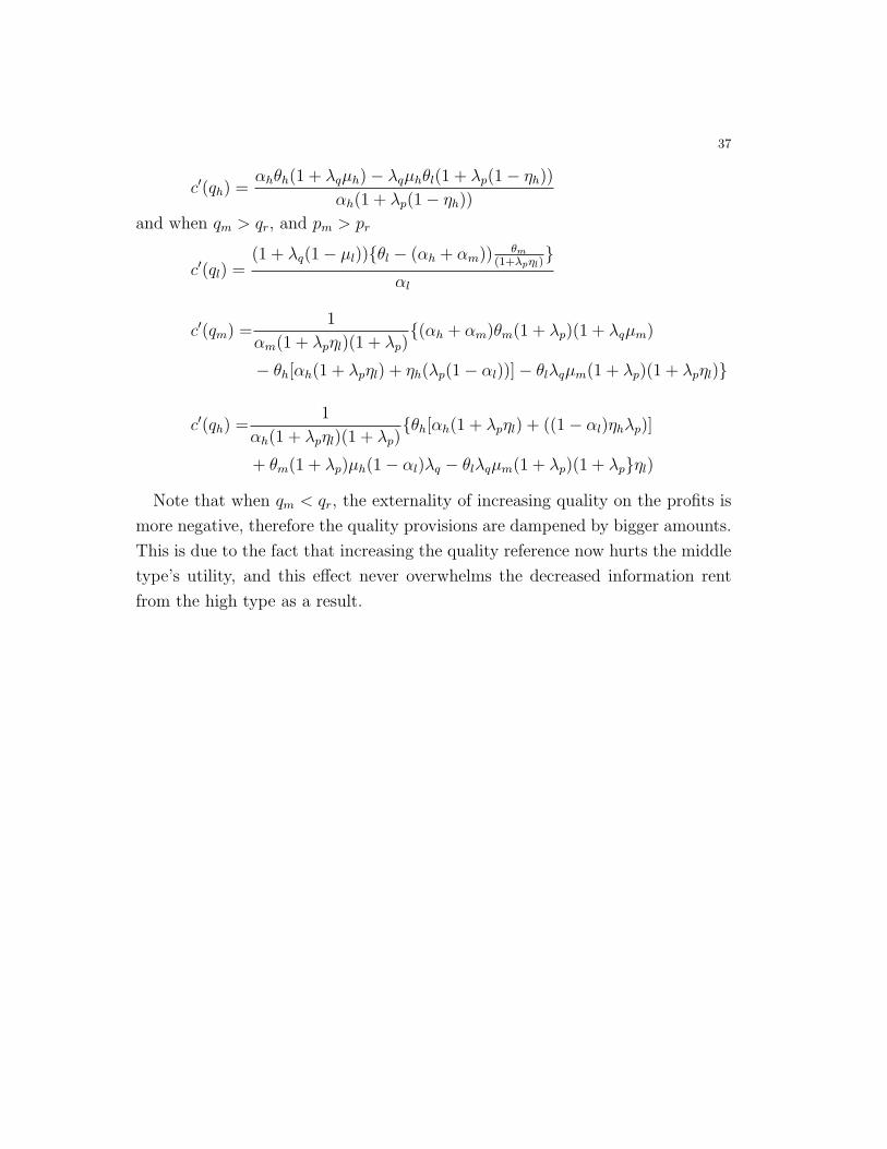
37

c′(qh) =αhθh(1 + λqµh)− λqµhθl(1 + λp(1− ηh))

αh(1 + λp(1− ηh))

and when qm > qr, and pm > pr

c′(ql) =(1 + λq(1− µl)){θl − (αh + αm)) θm

(1+λpηl)}

αl

c′(qm) =1

αm(1 + λpηl)(1 + λp){(αh + αm)θm(1 + λp)(1 + λqµm)

− θh[αh(1 + λpηl) + ηh(λp(1− αl))]− θlλqµm(1 + λp)(1 + λpηl)}

c′(qh) =1

αh(1 + λpηl)(1 + λp){θh[αh(1 + λpηl) + ((1− αl)ηhλp)]

+ θm(1 + λp)µh(1− αl)λq − θlλqµm(1 + λp)(1 + λp}ηl)

Note that when qm < qr, the externality of increasing quality on the profits is

more negative, therefore the quality provisions are dampened by bigger amounts.

This is due to the fact that increasing the quality reference now hurts the middle

type’s utility, and this effect never overwhelms the decreased information rent

from the high type as a result.

38 A.YESIM ORHUN

Figure 1. Compromise Effect

Figure 2. Capturing Compromise Effect

39

Figure 3. Enhancement and Detraction

Figure 4. Capturing Enhancement

40 A.YESIM ORHUN

Figure 5. Asymmetric Dominance and Asymmetric Advantage

Figure 6. Capturing Asymmetric Dominance

41

Figure 7. Local Changes in the Intermediate Option