Queueing Dynamics and State Space Collapse inFragmented Limit Order Book Markets

Costis MaglarasGraduate School of Business

Columbia Universityemail: c.maglaras@gsb.columbia.edu

Ciamac C. Moallemi∗Graduate School of Business

Columbia Universityemail: ciamac@gsb.columbia.edu

Hua ZhengGraduate School of Business

Columbia Universityemail: hzheng14@gsb.columbia.edu

Current Version: July 10, 2017

Abstract

In modern equity markets, participants have a choice of many exchanges at which to trade.Exchanges typically operate as electronic limit order books under a “price-time” priority ruleand, in turn, can be modeled as multi-class FIFO queueing systems. A market with multipleexchanges can be thought as a decentralized, parallel queueing system. Heterogeneous tradersthat submit limit orders select the exchange, i.e., the queue, in which to place their orders bytrading off financial considerations against anticipated delays until their orders may fill. Theselimit orders can be thought as jobs waiting for service. Simultaneously, traders that submitmarket orders select which exchange, i.e., queue, to direct their order. These market orderstrigger instantaneous service completions of queued limit orders. In this way, the “server” is theaggregation of self-interested, atomistic traders submitting market orders.

Taking into account the effect of investors’ order routing decisions across exchanges, wefind that the equilibrium of this decentralized market exhibits a state space collapse property,whereby: (a) the queue lengths at different exchanges are coupled in an intuitive manner; (b) thebehavior of the market is captured through a one-dimensional process that can be viewed as aweighted aggregate queue length across all exchanges; and (c) the behavior at each exchange canbe inferred via a mapping of the aggregated market depth process that takes into account theheterogeneous trader characteristics. The key driver of this coupling phenomenon is anticipateddelay, as opposed to the queue lengths themselves. Analyzing a TAQ dataset for a sample ofstocks over a one month period, we find empirical support for the predicted state space collapse.Separately, using the data before and after Nasdaq’s natural fee-change experiment from 2015we again find agreement between the observed market behavior and the model’s predictionsaround the fee change.

1. Introduction

Motivation. Modern equity markets are highly fragmented. In the United States alone there are

over a dozen exchanges and about forty alternative trading systems where investors may choose∗The second author acknowledges the support of NSF Grant CMMI–1235023.

1

to trade. Market participants, including institutional investors, market makers, and opportunistic

investors, interact within today’s high-frequency, fragmented marketplace with the use of electronic

algorithms that differ across participants and types of trading strategies. At a high level, they

dynamically optimize where, how often, and at what price to trade, seeking to achieve their own

best execution objectives while taking into account short term differences or opportunities across

the various exchanges. Exchanges function as electronic limit order books, typically operating under

a “price-time” priority rule: resting orders are prioritized for trade first based on their respective

prices, and then, at a given price, according to their time of arrival, i.e., in first-in-first-out (FIFO)

order. The dynamics of an exchange can be understood as that of a multi-class system of queues,

where each queue is associated with a price level. Job arrivals into these queues correspond to new

limit orders posted at the respective prices. Market orders trigger executions which, in queueing

system parlance, correspond to service completions.

The market, consisting of multiple exchanges, can be viewed as a stochastic network that evolves

as a collection of parallel, multi-class queueing systems. Figure 1 depicts one side of the market at

one price level. Heterogeneous, self-interested traders optimize where to route their limit and market

orders, coupling the dynamics of these parallel queues. Studying the interaction effects between

market fragmentation and high-frequency, optimized order routing decisions is an important issue

in understanding market behavior and trade execution, and is the main focus of this paper.1

At a point in time, conditions at the exchanges may differ with respect to the best bid and offer2

price levels, the market depth at various prices, recent trade activity, etc. Exchanges publish real-

time information for each security that allow investors to know or compute these quantities. These,

in turn, imply differences in a number of execution metrics across exchanges, such as the probability

that an order will be filled, the expected delay until such a fill, or the adverse selection associated

with a fill. Exchanges also differ with respect to their underlying economics. Under the “make-take”

pricing that is common, exchanges typically offer a rebate to liquidity providers, i.e., investors that

submit limit orders that “make” markets when their orders get filled; simultaneously, exchanges

charge a fee to “takers” of liquidity that initiate trades using marketable orders that transact

against posted limit orders. Fees range in magnitude, and are typically between −$0.00103 and1This paper will adopt the terminology encountered in financial markets, both to help describe this domain that

may be of independent interest to the stochastic modeling community, and to highlight the close connection betweenthe model, the associated results, and the underlying application.

2The bid is the highest price level at which limit orders to buy stock of a particular security are represented atan exchange; the offer or the ask is the lowest price level at which limit order to sell stock are represented at theexchange; the bid price is less than the offered price. The difference between the offer and the bid is referred to asthe spread. Exchanges may differ in their bid and offer price levels, and at any point in time the highest bid and thelowest offer among all exchanges, comprise the National Best Bid and Offer (NBBO).

3Negative fees occur on “inverted” exchanges where payments are made to liquidity takers.

2

$0.0030 per share traded. Since the typical bid-offer spread in a liquid stock is $0.01, the fees

and rebates are a significant fraction of the overall trading costs, and material in optimizing over

routing decisions. Most retail investors do not have access to this information, but essentially all

institutional investors and market makers — that, taken together, account for almost all trading

activity — have access and do make use of this information. They employ so-called “smart order

routers” that take into account real-time state information and formulate an order routing problem

that considers various execution metrics in order to decide whether to place a limit order or trade

immediately with a market order, and accordingly to which venue(s) to direct their order. Investors

are heterogeneous; specifically they differ with respect to the way that they trade off metrics such

as price, rebates, and delays, primarily driven by their intrinsic patience until they fill their order.

From a stochastic modeling viewpoint, the aforementioned system consists of parallel multi-class

queues (the exchanges) that differ in their economics and anticipated delays. These subsystems

are decentralized. Moreover, service capacity is neither centrally controlled nor dedicated as is

typical in production or service systems. Instead, it emerges by aggregating individual market

orders (service completions) directed to different queues, themselves optimizing over heterogeneous

trade-offs between economics and operational metrics related to queueing effects.

Summary of results. First, the paper offers a novel model for order routing in fragmented

markets that takes into account queueing phenomena in limit order books, as well as the atomistic

limit order placement and market order (service completions) routing decisions. This model ex-

plicitly leverages ideas for the economics of queues literature to capture the tradeoff between delay

and rebate capture in the routing decision of limit orders. It also incorporates, in a reduced-form,

the self-interested routing decisions of marker orders that comprise the service completion process.

The resulting model is a two-sided parallel queue system. The self-interested nature of the ser-

vice completion process may be of independent interest; e.g., one possible application might be in

modeling personnel that work in retailing that may strategize over which customer to help next,

or self-interested drivers in a ride hailing network that can select where to drive their car when

they are not serving customers. The formulation of the limit order routing problem, importantly,

incorporates the heterogeneous preferences of the various market participants with respect to the

way they trade off delays (time) with the anticipated rebate (money).4

Second, from a methodological viewpoint, we study a deterministic and continuous fluid model

associated with the above system, that takes into account the routing decisions of atomistic limit4 Investors differ in the urgency with which they seek to execute their orders, which is, in turn, captured by the

parameters of their selected execution algorithm, e.g., an algorithm with a target participation rate, say 5%, 10% or20% of the market volume. Such an urgency parameter affects how long will a trader be willing to wait until a limitorder would be filled, which would affect the order placement decision.

3

order placements and market orders (service completions). The key result is to characterize the

structural form of the equilibrium state of this fluid model and derive a form of state space collapse

(SSC) property.The market equilibrium and SSC are not the result of the price protection mecha-

nism5 imposed in the U.S. equities market. Rather, they arise out of order routing decisions among

exchanges that offer to trade at the same price level but at different (rebate, delay) combinations.

We characterize this coupling effect that yields a strikingly simplifying property whereby the be-

havior of the multi-dimensional market reduces to that of a one-dimensional system expressed in

terms of what we refer to as workload, which is an aggregate measure of the total available liquid-

ity. In equilibrium, the workload is a sufficient statistic that summarizes the state of the market.

The expected delay at each exchange is proportional to the workload, where the proportionality

constant depends on exchange specific parameters. In equilibrium, if one exchange is experiencing

long delays, then the other exchanges will also be experiencing proportionally long delays. Con-

versely, if (out of equilibrium) one exchange has temporarily an atypically small associated delay

relative to its cost structure, the new order flow will quickly take advantage of that delay/cost

opportunity and erase that difference.6 For N = 2 exchanges, we use a geometric argument to

prove that the fluid model transient starting from an arbitrary initial condition converges to the

equilibrium state in finite time. We conjecture that a similar argument carries through when there

are N > 2 exchanges. The specific form of our SSC result depends on our assumptions regarding

the routing of limit and market orders, as is typical of such results. The parameters that describe

the heterogeneity of trader preferences and the fees and rebates at the various exchanges dictate

the resulting equilibrium state.

Third, we empirically verify the state space collapse property for a sample of TAQ data for

the month of 9/2011 for the 30 securities that comprise the Dow Jones Index. While all being

liquid stocks, these securities differ in their trading volumes, price, volatility, and spread. Our

methodological results suggest certain testable hypotheses, most notably regarding the effective

dimensionality of the market dynamics, the linear relation between the expected delays across

exchanges, and the relation between expected delays and market-wide workload. These empirical

findings are summarized in § 4 and find statistical support for the SSC prediction of our model,

despite its stylized assumptions. To our knowledge, this seems to be one of the first empirical

verifications of SSC in a real and complex stochastic processing system.

The 1-dimensional workload characterization seems to offer a tractable model for downstream5Regulation NMS, see http://www.sec.gov/spotlight/regnms.htm.6 A simpler version of this effect is the familiar picture we encounter in highway toll booths or supermarket

checkout lines, where people join the shortest queue; in our model choice behavior is more intricate, and depends oneconomics, anticipated delays, as well as trader heterogeneity.

4

analysis of questions that pertain to exchange competition (e.g., how to set fees or associated

volume tiers), policy questions that may affect the routing decision problem or impose exogenous

transaction costs (e.g., a transaction tax), and market design questions (e.g., whether the co-

existence of competing, differentially priced exchanges is beneficial from a welfare perspective).

To that effect, one of its predictions is that if a high-rebate exchange were to lower its rebate and

fee, the market response would be such that the queues and trading volumes would equilibriate

in such a way so as to reduce the anticipated delay for limit orders placed in that exchange when

compared to the delays encountered in other exchanges. Lower fees would make the exchange

more attractive for the submission of market orders, possibly increasing volume. On the other

hand, lower rebates would reduce the attractiveness of the exchange for placing limit orders, which

would, all other things kept constant, leading to a reduction in queue sizes. Small queues, in turn,

discourage market order activity. Our model predicts the above opposing effects would balance

out through their effect on trading delays, which should decrease, as traders will be willing to wait

less to receive the smaller rebate. In 2015, NASDAQ ran a pilot experiment to precisely explore

this issue for a sample of 14 stocks. In § 4.4 we find strong statistical support for our model’s

prediction. Our study complements several industry reports that studied market data before and

after this natural experiment, e.g., Hatheway (2015a,b); Pearson (2015) that had primarily focused

on descriptive statistics and ex-ante / ex-post comparisons of volume and depth comparisons.

Literature Survey. There are two strands of literature that we briefly review. The first is

on market microstructure and financial engineering, and focuses on the structure and behavior of

limit order books. Apart from the classical market microstructure models, such as those proposed

by Kyle (1985), Glosten and Milgrom (1985) and Glosten (1987), our paper is related to several

strands of work. First is the set of papers that report on empirical analyses of the dynamics of

exchanges that operate as electronic limit order books, such as Bouchaud et al. (2004), Griffiths

et al. (2000), and Hollifield et al. (2004) and the review article Parlour (2008). Related to the above

work, there is a body of literature that studies the effect of adverse selection, which factors in order

placement decisions; c.f., Keim and Madhavan (1998), Dufour and Engle (2000), Holthausen et al.

(1990), Huberman and Stanzl (2004), Gatheral (2010), and Sofianos (1995).

Second, there are several papers that study market fragmentation, exchange competition and

their effect on market outcomes dating back to the work of Hamilton (1979), Glosten (1994, 1998),

and, more recently, Bessembinder (2003) and Barclay et al. (2003). A number of papers, including

O’Hara and Ye (2011), Jovanovic and Menkveld (2011), and Degryse et al. (2011), empirically

study the impact of exchange competition on available liquidity and market efficiency. Biais et al.

(2010) and Buti et al. (2011) consider the impact of differences in tick-size on exchange compe-

5

tition, while in the markets we consider, the tick-size is uniform. Foucault et al. (2005) describe

a theoretical model to understand make-take pricing when monitoring the market is costly. Mali-

nova and Park (2010) empirically study the introduction of make-take rebates and fees in a single

market. Foucault and Menkveld (2008) studies the impact of smart order routing on market be-

havior in a setting with two exchanges and focusing, however, on smart order routing decisions by

traders submitting market orders aiming to optimize their execution price (i.e., in a setting where

exchanges operate without a price protection mechanism, like Reg NMS that applies to the U.S.

equities market, that would eliminate the opportunity from such routing decisions); their paper

does not consider the routing decisions of limit orders, and disregards queueing effects. van Kervel

(2012) considers the impact of order routing in a setting where market makers place limit orders on

multiple exchanges simultaneously so as to increase execution probabilities. Their analysis ignores

economic and execution delay differences between venues. Sofianos et al. (2011) discuss smart order

placement decisions in relation to their all-in cost, introducing similar considerations to the ones

explored in this paper. More recently, Cont and Kukanov (2013) studied a smart order routing

control problem, where a trader decides how to split a non-infinitesimal order size across multiple

venues, taking into account the delay and rebate differences across exchanges and operating under a

control horizon T . Our model considers traders that submit infinitesimal order sizes, so the decision

of how to split their order is not relevant, but they are heterogeneous in terms of how they trade off

delay with rebates; our model also considers the routing of market orders and tries to characterize

the (stylized) market equilibrium.

Third, there is a growing body of work that develops models of limit order book dynamics

and studies optimal execution problems. Obizhaeva and Wang (2006), Rosu (2009), Alfonsi et al.

(2010), Parlour (1998), treat the market as one limit order book and use a model of market impact

and abstracts away queueing effects. The high-frequency behavior of limit order books can probably

be best modeled and understood as that of a queueing system. This connection has been explored

in recent work, starting with Cont et al. (2010); see also Maglaras et al. (2014), Cont and Larrard

(2013), Lakner et al. (2013), Blanchet and Chen (2013), Stoikov et al. (2011), Guo et al. (2013),

and Lakner et al. (2014); this set of papers does not consider fragmentation.

The second strand of literature related to our work is on stochastic modeling and relates to the

asymptotic analysis tools that motivate our method of analysis and the area of queueing systems

with strategic consumers. So-called equivalent workload formulations and the associated idea of

state space collapse arise in stochastic network theory in the context of their approximate Brownian

model formulations. This idea has been pioneered by the work of Harrison (1988) and Harrison

(2000). Workload fluid models were introduced in Harrison (1995). The condition that guarantees

6

that parallel server systems exhibit SSC down to one-dimensional systems was introduced by Har-

rison and Lopez (1999), and two papers that establish SSC results with optimized routing of order

arrivals are Stolyar (2005) and Chen et al. (2010). We model market order routing decisions via a

reduced form state dependent service rate process. Mandelbaum and Pats (1995) derive fluid and

diffusion approximations for such queues. Our analysis is itself deterministic, building on ideas and

tools from the asymptotic analysis of queues. We do not provide a limit theorem to justify the

deterministic fluid model we postulate as the system model, but instead focus on its analysis and

implications. SSC results tend to be pathwise properties, established via an asymptotic analysis

after an appropriate rescaling of time. In our system, arrival rates of limit and market orders vary

stochastically over time on a slower time scale than that of the transient fluid model dynamics.

An asymptotic analysis on the slower time scale of the event rate variations, in the spirit of the so

called Pointwise-Stationary-Fluid-Models (PSFM), would establish such a pathwise SSC property

by exploiting the transient fluid model results of this paper. Standard machinery for establishing

such results either exploit the work by Bramson (1998) or Bassamboo et al. (2004). Our model

seems to satisfy the key requirements that one would need to derive the PSFM and as a result the

sample path version of the SSC property, but we will not pursue this in this paper apart from a

short discussion in §3.5.

Optimal order placement decisions are made according to an atomistic choice model as per

Mendelson and Whang (1990). In the context of queueing models with pricing and service com-

petition, there are several papers including those of Luski (1976), Levhari and Luski (1978), and

Li and Lee (1994). and Lederer and Li (1997). Cachon and Harker (2002) and So (2000) analyze

customer choice models that divert from the lowest cost supplier under M/M/1 system models.

Allon and Federgruen (2007) studied the competing supplier game in a setting where the offered

services are partial substitutes. An extensive survey is provided in Hassin and Haviv (2003).

Most of the above papers look at static rules, where consumers make decisions based on steady-

state expected delays. Chen et al. (2010) considers competing suppliers and arriving consumers

making decisions based on real-time information, like in our model, but where each supplier has his

own dedicated processing capacity; the resulting dynamics are different and only couple through

order arrivals. The nature of the service completion process that emerges as the aggregation of

infinitesimal self-interested contributions appears novel viz the existing literature. Finally, Plam-

beck and Ward (2006) study an assemble-to-order system, that involves a two-sided market fed by

product requests on one side and raw materials on the other, but such systems allow queueing on

both sides and the flow of material is controlled by the system manager. Caldentey et al. (2009);

Gurvich and Ward (2014) study the dynamics of matching queues.

7

2. Model

We propose a stylized model of a fragmented market consisting of N distinct electronic limit order

books simultaneously trading a single underlying asset. The model will take the form of a system of

parallel FIFO queues; new price and delay sensitive jobs arrive over time and optimize their routing

decisions; self-interested agents arrive over time and optimize where to route their market order

that triggers an instantaneous service completion at the respective queue (i.e., this routing decision

happens at the “end of the service time”). Our focus is to understand the effect of optimized order

routing decisions on the interaction between multiple limit order books. We make a number of

simplifying assumptions that aid the tractability of our model studied in Sections 2–3.

One-sided market. We model one side of the market, which, without loss of generality, choose

to be the bid side, where investors post limit orders to buy the stock and wait to execute against

market orders directed by sellers.

Top-of-book only. Limit orders are distinguished by their limit price. We only consider limit

orders at each exchange posted at the national best bid price, the highest bid price available across

all exchanges – the “top-of-book.” A profit-maximizing seller would only choose to trade at the top

of book, and, in fact, in the United States, this is enforced de jure by SEC Regulation NMS.

Fluid model. We consider a deterministic fluid model, or “mean field” model, where the discrete

and stochastic order arrival processes are replaced by continuous and deterministic analogues,

where infinitesimal orders arrive continuously over time at a rate that is equal to the instantaneous

intensity of the underlying stochastic processes. This model can be justified as an asymptotic limit

using the functional strong law of large numbers in settings where the rates of order arrivals grow

large but the size of each individual order is small relative to the overall order volume over any

interval of time. It is well suited for characterizing transient dynamics in such systems, which is the

time scale over which queue lengths drain or move from one configuration to another; this is also

the relevant time scale in order routing decisions. For liquid securities, orders arrive on a time scale

measured in milliseconds to seconds, while queueing delays are of the order of seconds to minutes.

Constant arrival rates. Market activity exhibits strong time-of-day effects, typically over longer

time scales (e.g., minutes to hours) than what we focus on. The analysis of the next section assumes

that arrival rates are constant, and do not depend on time or the state at the exchanges.

Our model is illustrated in Figure 1. For each of the N exchanges, there is a (possibly empty)

queue of resting limit orders at the national best bid price. The vector of queue lengths at time t

is denoted by Q(t) ,(Q1(t), Q2(t), . . . , QN (t)

)∈ RN+ .

8

exchange 1

exchange 2

exchange N

Λ ?

market order(“exchange 0”)

optimizedlimit order flow

λ1

λ2

λn

dedicatedlimit order flow

µ?

market order flow

Figure 1: A one-sided, top-of-book model of multiple limit order books. Limit orders (i.e., jobs) arriveto each exchange (modeled by the respective queues) in (a) dedicated streams and (b) optimized limitorder placement decisions. Liquidity is removed through the arrival of decentralized, self-interestedmarket orders, acting as service completions.

2.1. Limit Order Routing

A continuous and deterministic flow of investors arrives to the market with the intent of posting

an infinitesimal limit order. This flow consists of two types:

Dedicated limit order flow arrives at rate λi ≥ 0 and is destined to exchange i, independent of

the state Q(t) at the various exchanges. This flow could represent, for example, investors that may

not have the ability to route orders to all exchanges, or to make real-time order routing decisions.

Optimized limit order flow arrives at a rate Λ > 0. Each infinitesimal investor observes the

state of the market, Q(t), and optimizes over where to route the associated infinitesimal order, or,

if conditions are unfavorable, not to leave a limit order and to trade instead with a market order

at the offered (other) side of the market; this option is denoted by i = 0.

Once a limit order is posted at a particular exchange, it remains queued until it is executed

against an arriving market order. This disregards order cancellations. Cancellations occur, for

example, when time sensitive orders “deplete” their patience and cancel to cross the spread and

trade with a market order; when investors perceive an increased risk of adverse selection; etc. This

assumption simplifies the order routing decision and leads to a tractable analysis.7

7Cancellations are common. Typical models of cancellations assume either that orders cancel according to anexponential alarm clock leading to a cancelation process that is proportional to the queue length, or that there isconstant drift out of the bid queue due to cancelations, independent of the queue length. The first offers a reasonablemodel for orders generated by algorithmic trading strategies used by institutional investors, such as VWAP, POV,etc., but it is not a good way to model the behavior of orders posted by market makers. The latter account for most ofthe orders in the queue, and, indeed, they tend to cancel using a state-dependent criterion as opposed to a time-based

9

Expected delay. All things being equal, an investor would prefer a shorter delay until an order

gets executed. Apart from price risk considerations, this is often due to exogenous constraints on

the speed at which the order needs to get filled; in many instances, a limit order may be a “child

order” that is part of the execution plan of a larger “parent order,” which itself needs to be filled

within a limited time horizon and under some constraints on its execution trajectory defined by its

“strategy.” As will be seen in Section 4, the expected delays vary in the range of 1 to 1000 seconds.

Given Qi(t) and a market order arrival rate µi > 0, the expected delay in exchange i is

(1) EDi(t) ,Qi(t)µi

.

The µi’s are assumed to be known, and, indeed, in practice, they can be approximated by observing

recent real-time trading activity at each exchange. When the investor decides not to place a limit

order but instead trade with a market order, the order is immediately executed and ED0 , 0.

Rebates. Exchanges provide a monetary incentive to add liquidity by providing rebates for each

limit order that is executed. Over time, these have varied by exchange from −$0.0010 (a negative

liquidity rebate is, in fact, a fee charged to liquidity providers) to $0.0030 per share traded. As

mentioned earlier, they are significant in magnitude when compared to the bid-ask spread of a

typical liquid stock of $0.01 per share, and represent an important part of the trading costs that

influence the order routing decisions. All things being equal, investors prefer higher rebates.

We denote the liquidity rebate of exchange i by ri. In the case where the investor chooses to

take liquidity (i = 0), a market order will, relative to a limit order, involve both paying the bid-offer

spread and paying a liquidity-taking fee. The sum of these payments is denoted by r0 < 0.

In practice, order placement decisions depend on various factors in addition to the ones described

above. For example, an investor may have explicit views on the short-term movement of prices

(“short-term alpha”), and these can be relevant for the placement of limit orders; be sensitive to

adverse selection, or the anticipated price movement after the execution of a limit order; etc. In

order to maintain tractability, we will focus on the direct trade-off between financial benefits and

delays. We will denote the financial benefit per share traded associated with exchange i by ri and

refer to it as the effective rebate; this includes the direct exchange rebate but possibly incorporates

other financial considerations. All else being equal, a higher effective rebate is preferable.

We denote the opportunity set of effective rebate and delay pairs encountered by an investor

arriving at time t by E(t) ,{(ri,EDi(t)) : 0 ≤ i ≤ N

}. Investors are heterogeneous with respect to

one. The simple cancellation models described above would underestimate the expected delay until an order will getfilled in liquid securities. The incorporation of the different cancellation behaviors, timer-based and state-dependent,complicates the dynamics of the queue but leads to better agreement with data; Kukanov and Maglaras (2015).

10

their way of trading off rebate against delay. Each investor is characterized by its type, denoted by

γ ≥ 0, that is assumed to be an independent identically distributed (i.i.d.) draw from a cumulative

distribution function F (·), that is differentiable and has a continuous density function, and selects

a routing decision i∗(γ) so as to maximize his “utility” according to the rule 8

(2) i∗(γ) ∈ argmaxi∈{0,1,...,N}

γri − EDi(t).

In other words, γ is a trade-off coefficient between price and delay, with units of time per dol-

lar, that characterizes the type of the heterogeneous investors. Given the range of rebates and

expected delays, this trade-off coefficient should roughly be in the range of 1 to 104 seconds per

$.01. Heterogeneity in γ across investors is an important feature of our model, which captures the

practical reality that investors differ in their urgency to execute their orders, which, in turn, affects

their patience and limit order placement behavior, implicitly or explicitly (through their choice of

algorithmic trading strategy and associated parameters; cf. Footnote 4). If at the time of an order

arrival the prevailing delays are long, then some investors may choose not to post a limit order

altogether but instead cross the spread and execute their order with a market order (the exchange

designated “0” in our model.

An equivalent formulation to (2), commonly used in the economic analysis of queues, is to

convert the delay into a monetary cost by multiplying it with a delay sensitivity parameter. Yet

another alternative interpretation would assume that investors differ in terms of their expected

delay tolerance, i.e., the maximum length of time they are willing to wait for an order to be filled.

Given an estimate of the anticipated delays, investors with relatively longer delay tolerance would

try to place orders in high rebate exchanges, whereas others with shorter delay tolerance would

sacrifice high rebates and place their orders in exchanges with shorter delays (and lower rebates)

so as to maximize the probability that their order will get filled in time. Such a reformulation of

(2) would still involve a fundamental trade-off between monetary rebate weighed against measures

of delay or execution risk. Overall, while (2) is a simplified criterion, it captures the fundamental

trade-off between time and money, and it will ultimately yield structural results that are consistent

with our empirical analysis.

2.2. Market Order Routing

Investors arrive to the market continuously at an aggregate rate µ > 0, seeking to sell an infinites-

imal quantity of stock instantaneously via a market order. For an investor who arrives to the8The criterion (2) is “static.” In practice, order routing decisions are “dynamic,” i.e., done and updated over the

lifetime of the order in the market.

11

market at time t when the queue length vector is Q(t), the routing decision is restricted to the set

of exchanges {i : Qi(t) > 0}. One important factor influencing this decision is that each exchange

charges a fee for taking liquidity, and these fees vary across exchanges. Typically the fee at an

exchange is slightly higher than the rebate, and the exchange pockets the difference as a profit.

Fee and rebate data is given in Section 4. For the purposes of this discussion, we assume that the

fee on exchange i is equal to the rebate ri. Since a market order executes without any delay, it is

natural to route it to exchange i∗ so as to minimize the fee paid:

(3) i∗ ∈ argmini∈{1,...,N}

{ri : Qi(t) > 0}.

In practice, routing decisions may differ from those predicted by fee minimization for a number

of reasons: (a) Real order sizes are not infinitesimal, and to trade a significant quantity one may

need to split an order across many exchanges. (b) If an investor observes that liquidity is available

at an exchange, due to latency in receiving market data information or in transmitting the market

order to the exchange, that liquidity may no longer be present by the time the investor’s market

order reaches the exchange. This is accentuated if there are only a few limit orders posted at an

exchange. Both (a) and (b) create a preference for longer queue lengths. (c) If an exchange has

very little available liquidity, “clearing” the queue of resting limit orders is likely to result in greater

price impact. (d) There may be other considerations involved in the order routing decision, such

as different economic incentives between the agent making the order routing decision and the end

investor. All of these effects point to a more nuanced decision process than the fee minimization

suggested by (3), which we will capture through a reduced form “attraction” model that is often

used in marketing to capture consumer choice behavior. Specifically, given Q(t), the instantaneous

rate at which market orders to sell arrive at exchange i is denoted by µi(Q(t)) given by

(4) µi(Q(t)) , µ fi(Qi(t))∑Nj=1 fj(Qj(t))

.

Equation (4) specifies that the fraction of the total order flow µ that goes to exchange i is propor-

tional to the attraction function fi(Qi(t)), with fi(0) = 0, i.e., market orders will not route to an

exchange i with no liquidity. The discussion above suggests that fi(·) is an increasing function of

the queue length Qi, and a decreasing function of the size of the fee charged by the exchange.

In the remainder of this paper, we use a basic linear model of attraction that specifies

(5) fi(Qi) , βiQi,

12

where βi > 0 is a coefficient that captures the attraction of exchange i per unit of available

liquidity. We posit (but our model does not require) that the βi’s be ordered inversely to the fees

of the corresponding exchanges. We will revisit this empirically in Section 4.

2.3. Fluid Model

The deterministic fluid model equations are the following: for each exchange i,

(6) Qi(t) = Qi(0) + λit+ Λ∫ t

0χi(Q(s)

)ds−

∫ t

0µi(Q(s)

)ds.

The quantity χi(Q(·)

)denotes the instantaneous fraction of arriving limit orders that are placed

into exchange i, defined as

(7) χi(Q(t)

),∫Gi(Q(t)

) dF (γ),

where Gi(Q(t)

)denotes the set of optimizing limit order investor types γ that would prefer exchange

i, i.e., the set of all γ ≥ 0 with γri− EDi(t) ≥ γrj − EDj(t) for all j 6= i, given the expected delays

ED0(t) = 0 and EDj(t) = Qj(t)/µj(Q(t)

), for j = 1, . . . , N , implied9 by Q(t).

3. Equilibrium Analysis

Suppose that at some point in time a high rebate exchange has a very short expected delay relative

to other exchanges. Then, the routing logic in (2) will direct many arriving limit orders towards

this exchange, increasing delays and erasing its relative advantage viz the other exchanges. This

type of argument suggests that queue lengths will evolve over time and eventually converge into

some equilibrium configuration where no exchange seems to have a relative advantage with respect

to its rebate/delay trade-off taking into account the investors’ heterogeneous preferences and the

differences in the fees and rebates across exchanges.

Expressing (6) in differential form, we have that Qi(t) = λi + Λχi(Q(t)

)− µi

(Q(t)

), for i =

1, . . . , N . Denoting such an equilibrium queue length vector by Q∗, we have that:

(8) λi + Λχi(Q∗) = µi(Q∗), i = 1, . . . , N.9Here, we employ a “snapshot” estimate of expected delays that is consistent with our definition (1) and is often

used in practice. This disregards the fact that Q(t) and, as a result µi(Q(t)), may change over time, which wouldnaturally affect the delay estimate. In what follows, we will mainly be concerned with the behavior of the system inequilibrium, where Q(t) is constant and this distinction is not relevant.

13

These equations are coupled through the market order rates µi(Q∗) and the aggregated routing

decisions given by χi(Q∗) that take into account investor heterogeneity.

3.1. Equilibrium Definition

For each possible price-delay trade-off coefficient γ ≥ 0, πi(γ) denotes the fraction10 of type γ

investors who post limit orders to an exchange if i ∈ {1, . . . , N}, or choose to use a market order if

i = 0. We require that the routing decision vector π(γ) ,(π0(γ), π1(γ), . . . , πN (γ)

)satisfy

(9) πi(γ) ≥ 0, ∀ i ∈ {0, 1, . . . , N};N∑i=0

πi(γ) = 1.

Denote by π ,(πi(γ)

)γ∈R+

a set of routing decisions across all investor types, and let P denote

the set of all π where π(γ) is feasible for (9), for all γ ≥ 0, and where each πi(·) is a measurable

function over R+. We have suppressed the dependence of π on the rate parameters (λ,Λ, µ) and

the queue length vector. We propose the following definition of equilibrium:

Definition 1 (Equilibrium). An equilibrium (π∗, Q∗) ∈ P×RN+ is a set of routing decisions and queue

lengths that satisfies:

(i) Individual Rationality: For all γ ≥ 0, the routing decision π∗(γ) for type γ investors is an

optimal solution for

(10)maximize

π(γ)π0(γ) γr0 +

N∑i=1

πi(γ)(γri −

Q∗iµi(Q∗)

)

subject to πi(γ) ≥ 0, ∀ i ∈ {0, 1, . . . , N};N∑i=0

πi(γ) = 1.

(ii) Flow Balance: For each exchange i ∈ {1, . . . , N}, the total flow of arriving market orders

equals the flow of arriving limit orders, i.e.,

(11) λi + Λ∫ ∞

0π∗i (γ) dF (γ) = µi(Q∗).

Assuming that queue lengths are constant and given by Q∗, the expected delay on each ex-

change i is given by Q∗i /µi(Q∗). The individual rationality condition (i) ensures that limit or-

ders are routed in a way that is consistent with (2). The flow balance condition, (ii), ensures

that inflows and outflows at each exchange are balanced and that the queue length vector Q∗

10We will typically expect that πi(γ) ∈ {0, 1}, i.e., all type γ investors will prefer a single exchange, unless thereare ties between exchanges.

14

remains stationary. Definition 1 is consistent11 with the informal system of equations (8) since

χi(Q∗) =∫∞

0 π∗i (γ) dF (γ).

3.2. State Space Collapse

Given a vector of queue lengths Q, define the workload to be the scaled sum of queue lengths

given by W ,∑Ni=1 βiQi. The workload captures the aggregate market depth across all exchanges,

weighted by the attractiveness of each exchange. Orders queued at attractive exchanges (high βi,

typically corresponding to low ri) are weighted more since these orders have greater priority to get

filled first, and, therefore, more greatly impact the delays experienced by arriving limit orders at

all exchanges. In fact, from (1) and (4), the expected delay on exchange i is given by

(12) EDi = W

µβi.

That is, the 1-dimensional workload is sufficient to determine delays at every exchange. Theorem 1

below establishes something stronger: in equilibrium, the queue length vector Q∗, which is the state

of the N -dimensional system can be inferred from the equilibrium workload W ∗. This is a notion

of state space collapse.

Theorem 1 (State Space Collapse). Suppose that the pair (π∗,W ∗) ∈ P × R+ satisfy

(i) π∗ is an optimal solution for

(13)

maximizeπ

∫ ∞0

{π0(γ) γr0 +

N∑i=1

πi(γ)(γri −

W ∗

µβi

)}dF (γ)

subject to πi(γ) ≥ 0, ∀ i ∈ {0, 1, . . . , N}, ∀ γ ≥ 0,N∑i=0

πi(γ) = 1, ∀ γ ≥ 0.

(ii) π∗ satisfies

(14)N∑i=1

(λi + Λ

∫ ∞0

π∗i (γ) dF (γ))

= µ.

11Strictly speaking, the informal definition (8) may not deal properly with situations where agents are indifferentbetween multiple routing decisions, while the formal Definition 1 handles this correctly. Under mild technical con-ditions we will adopt shortly (Assumption 1 and the hypothesis of Theorem 3) however, the mass of such agents iszero and the two definitions coincide.

15

Then, (π∗, Q∗) is an equilibrium, where for each exchange i 6= 0, Q∗ is defined by

(15) Q∗i ,(λi + Λ

∫ ∞0

π∗i (γ) dF (γ))W ∗

µβi.

Conversely, if (π∗, Q∗) is an equilibrium, define W ∗ , β>Q∗. Then, (π∗,W ∗) satisfy (i)–(ii).

Proof. Suppose that (π∗,W ∗) satisfy (i)–(ii). For Q∗ given by (15), we have that

β>Q∗ =∑i 6=0

W ∗

µ

(λi + Λ

∫ ∞0

π∗i (γ) dF (γ))

= W ∗.

Thus,

(16) W ∗

µβi= β>Q∗

µβi= Q∗iµi(Q∗)

.

Combining this with the fact that optimization problem in (i) is separable with respect to γ (i.e.,

it can be optimized over each π(γ) separately), it is clear that (π∗, Q∗) satisfies the individual

rationality condition (10). Further, rewriting (15),

λi + Λ∫ ∞

0π∗i (γ) dF (γ) = µ

βiQ∗i

W ∗= µ

βiQ∗i

β>Q∗= µi(Q∗).

Thus, (π∗, Q∗) satisfies flow balance condition (11), and (π∗, Q∗) is an equilibrium.

For the converse, suppose that (π∗, Q∗) is an equilibrium and W ∗ , β>Q∗. Then,

W ∗

µβi= β>Q∗

µβi= Q∗iµi(Q∗)

.

Given that (π∗, Q∗) satisfies (10), this implies that (π∗,W ∗) satisfy (i). Further, if we sum up all

N equations in (11), it is clear that (π∗,W ∗) satisfy (ii). �

Condition (i) of Theorem 1 implies individual rationality when faced with delays implied by the

workload W ∗, cf. (10) and (12). Condition (ii), is a market-wide flow balance equation. Given a

pair (π∗,W ∗) satisfying (i) and (ii), Q∗ is determined as a function of workload W ∗ through the

lifting map (15) that distributes the workload across exchanges in a way that takes into account

rebates, delays, and investor heterogeneity through the distribution F (·) of the trade-off coefficient

γ. The lifting map corresponds to Little’s Law: each queue length is equal to the corresponding

aggregate arrival rate (dedicated and optimized) times the equilibrium expected delay.

16

3.3. Equilibrium Characterization

Theorem 1 allows us to characterize the equilibrium behavior of N decentralized limit order books

through their 1-dimensional workload. The following assumption will turn out to be sufficient for

the existence of an equilibrium:

Assumption 1. Assume that

(i) The cumulative distribution function F (·) over the price-delay trade-off coefficients γ is non-

atomic with a continuous and strictly positive density on the non-negative reals.

(ii) The arrival rates (λ,Λ, µ) satisfy∑Ni=1 λi < µ < Λ +

∑Ni=1 λi.

(iii) Each exchange i ∈ {1, . . . , N} satisfies ri > r0.

The dedicated flow∑Ni=1 λi is not delay sensitive. Condition (ii) ensures that the queueing

system is stable (∑Ni=1 λi < µ) and leads to a non-trivial equilibrium where queue lengths are

non-zero (µ < Λ +∑Ni=1 λi). Condition (iii) says that if delays are zero, then the effective rebate

of a limit order is always preferable to the cost of crossing the spread and paying a fee to trade

with a market order, r0. Returning to condition (ii), given that µ < Λ +∑Ni=1 λi, one would expect

non-zero queue lengths to build up in the system to discourage some optimizing investors from

placing a limit order and instead trade with a market order. Intuitively, one expects this to be the

most impatient investors, i.e., those of type γ ≤ γ0, for some γ0, chosen to satisfy (14),

(17) Λ(1− F (γ0)

)+

N∑i=1

λi = µ.

Under conditions (i)–(ii) of Assumption 1, γ0 satisfying (17) exists and is uniquely determined by

(18) γ0 , F−1(

1− µ−∑Ni=1 λi

Λ

).

In order for all types γ ≤ γ0 not to submit limit orders, the routing criterion (2) requires that

(19) maxi 6=0

γ(ri − r0)− W ∗

µβi≤ 0,

for all γ ≤ γ0. Under Assumption 1(iii), the left side of (19) is increasing in γ. Hence, (19) is

satisfied if we ensure that type γ0 investors are indifferent between market orders and limit orders.

17

Lemma 1. Under Assumption 1, suppose that (π∗,W ∗) is an equilibrium and define γ0 by (18).

Then,

(20) maxi 6=0

γ0(ri − r0)− W ∗

µβi= 0.

Further, suppose that for a given W ∗, (20) holds, and for each exchange i, define

(21) κi , βi(ri − r0).

Then, an exchange i achieves the maximum in (20) if and only if i ∈ argmaxj 6=0 κj.

(The proof of the Lemma is provided in Appendix.) The quantity κi is related to the desirability

of exchange i from the perspective of a limit order investor; κi is high when βi is high (resulting in

low delay) or when ri is high (resulting in a high rebate). Lemma 1 suggests that maximizing κicharacterizes the behavior of type γ0 (the marginal) investors that are indifferent between choosing

between a market order and a limit order. We refer to exchanges that achieve this maximum as

marginal exchanges. Thus, given a marginal exchange i ∈ argmaxj 6=0 κj , according to Lemma 1,

γ0(ri − r0)− W ∗

µβi= 0,

and therefore the equilibrium workload is W ∗ = γ0µκi. Theorem 2, whose proof can be found in

the Appendix, summarizes the discussion above and characterizes the equilibrium.

Theorem 2 (Equilibrium Characterization). Under Assumption 1, define γ0 by (18). Suppose that

the pair (π∗,W ∗) ∈ P × R+ satisfy

(22) W ∗ , γ0µmaxi 6=0

κi,

and

(23)π∗0(γ) = 1, for all γ < γ0,

π∗i (γ0) = 0, for all i /∈ A∗(γ0) ∪ {0},

π∗i (γ) = 0, for all γ > γ0, i /∈ A∗(γ),

where A∗(γ) , argmaxi 6=0 γri−W ∗/µβi. Then, (π∗,W ∗) is an equilibrium, i.e., satisfies (13)-(14).

Conversely, suppose that (π∗,W ∗) ∈ P × R+ is an equilibrium, i.e., satisfies (13)-(14). Then,

W ∗ must satisfy (22) and π∗ must satisfy (23), except possibly for γ in a set of F -measure zero.

This characterization of the workload process and its dependence on model parameters can be

18

used as a point of departure to analyze market structure and market design issues, and competition

and welfare implications of the presence of many differentiated exchanges. Theorem 2 implies that

the equilibrium workload is unique, and that equilibrium routing policies are unique up to ties.

3.4. Convergence of Fluid Model to Equilibrium Configuration

We first establish uniqueness of the equilibrium queue length vector Q∗ in the next Theorem (its

proof is available in an extended version of the paper available at the authors’ websites), under the

following mild assumption:

Assumption 2. Assume that the effective rebates {ri, i 6= 0} are distinct, and, without loss of

generality, that the exchanges are labeled in an increasing order, i.e., r0 < r1 < · · · < rN .

Theorem 3 (Uniqueness of Equilibria). Under Assumptions 1 and 2, there is a unique equilibrium

queue length vector Q∗.

Next we establish that the fluid model queue length vector Q(t) converges to the unique equi-

librium vector Q∗ as t → ∞. As in Section 2.3, define Gi(W (t)

)⊂ R+ to be the set of optimizing

limit order investor types γ that would prefer exchange i given a workload level12 of W (t), i.e., the

set of all γ ≥ 0 with

γri −W (t)µβi

≥ γrj −W (t)µβj

, for all j /∈ {0, i}; γri −W (t)µβi

≥ γr0,

and the instantaneous fraction of arriving limit orders that are placed into exchange i as

(24) χi(W (t)

),∫Gi(W (t)

) dF (γ).

Under Assumptions 1 and 2, (24) can be rewritten as

(25) χi(W ) =

F

(WΓ+

i

µ

)− F

(WΓ−iµ

)if Γ+

i ≥ Γ−i ,

0 otherwise,

12Note that in Section 2.3, Gi(·) and χi(·) were defined to be functions of the vector of all queue lengths. However,since they depend on the queue length of each exchange only through the expected delay and therefore the workload,we will abuse notation and define these as functions of workload here.

19

where the constants Γ+i ,Γ

−i are defined by

Γ+i ,

minj>i

β−1j − β

−1i

rj − riif i < N ,

∞ if i = N ,Γ−i , max

{β−1i

ri − r0, max

0<j<i

β−1i − β

−1j

ri − rj

}.

Assumption 3. Suppose that, for all W > 0,

(26)N∑i=1

βidχi(W )dW

< 0.

Assumption 3 is essentially a local stability drift condition13 that is easy to verify, and takes

the form of a tail condition on F (·). Specifically, using (25), we have that:

(27)N∑i=1

βidχi(W )dW

=N∑i=1

(Γ+i

µf

(WΓ+

i

µ

)− Γ−i

µf

(WΓ−iµ

))I{Γ+

i ≥Γ−i },

where f is the density associated with F . A sufficient condition for Assumption 3 is that

(28) tΓ+i f(tΓ+

i ) < tΓ−i f(tΓ−i ),

for all t > 0 and 1 ≤ i ≤ N such that Γ+i > Γ−i . This expression can be easily verified in a particular

problem instance, and it is satisfied for sufficiently broad class of distributions.

Definition 2 (Elastic Distribution). The cumulative distribution function F is elastic if γf(γ) is a

strictly decreasing function over γ ≥ 0.

Examining (28), it is clear that elastic distributions will always satisfy Assumption 3. As an

example, note that decreasing generalized failure rate distributions; see, e.g., Lariviere (2006), are

included in the class of elastic distributions.

In general, even under Assumptions 1 and 2, the queue lengths Q(t) need not converge to

the unique equilibrium Q∗ — it is easy to construct numerical counterexamples. However, the13The workload process evolves according to the differential equation W (t) =

∑N

i=1 βiQi(t) =∑N

i=1 βiλi +Λ∑N

i=1 βiχi(W (t)

)−∑N

i=1 βiµi(Q(t)

), which is itself a function of W (t). In equilibrium, where W (t) = W ∗,

we have W (t) = 0, i.e., 0 =∑N

i=1 βiλi + Λ∑N

i=1 βiχi(W ∗)−∑N

i=1 βiµi(Q∗). Now, consider a small deviation from

equilibrium of the form Q(t) = (1 + ε)Q∗ where ε is a small constant. Using the fact that µi((1 + ε)Q∗

)= µi(Q∗),

the expression for W (t), and a Taylor approximation for small ε we get that W (t) =∑N

i=1 βiλi + Λ∑N

i=1 βiχi((1 +

ε)W ∗)−∑N

i=1 βiµi(Q∗)≈ ΛεW ∗

∑N

i=1 βidχi

(W∗)

dW. Assumption 3 guarantees that W (t) < 0 when ε > 0 and that

W (t) > 0 when ε < 0. That is, it is a necessary condition for local stability around W ∗. (Note that it not a sufficientcondition, since we only consider a restrictired form of perturbation in this discussion.) Assumption 3 extends thatcondition to the entire state space.

20

following theorem illustrates that the additional condition of Assumption 3 is sufficient to guarantee

convergence to equilibrium when there are N = 2 exchanges:

Theorem 4. Suppose that there are N = 2 exchanges. Under Assumptions 1–3, given arbitrary

initial conditions Q(0) ∈ RN+ , the queue lengths converge to the unique equilibrium Q∗.

(The proof of Theorem 4 is available in an extended version of the paper available at the

authors’ websites.) For N > 2, condition (26) is necessary for local stability of the equilibrium Q∗.

We conjecture that, as for N = 2, Assumption 3 is, in fact, also a sufficient condition when N > 2.

The state-space collapse result and its functional form hinge on the formulation of the order

routing models described in Sections 2.1 and 2.2. The primary drivers of the dimension reduction

are: (a) the desirability to place an order at a given queue is decreasing in its anticipated delay, and

(b) that the attractiveness of an exchange for an incoming market order is increasing in its queue

length. Both drivers seem plausible even under different models of order routing optimization logic

on both sides of the market, and one might expect these to lead to some form of state space collapse:

long queues would discourage new orders from joining while attracting more service completions,

thus reducing queue size; small queues would attract more arrivals but fewer service completions,

thus increasing queue size. For example, the same rationale holds if we replace the market order

routing model (4) with a model of the form µi(Q) , Mi + fi(Q), for each exchange i. Here,

each Mi ≥ 0 represents “dedicated” market order flow to exchange i that does not react to the

state of the system, while the fi(Q) term captures optimized order flow. The detailed form of the

equilibrium of such a system would not coincide with the one derived here, however, at a high level,

one would expect similar results under different modeling assumptions that satisfy (a)–(b).

3.5. Sketch of Pointwise Stationary Fluid Model

In the preceding analysis we have assumed that the event rate parameters (Λ, λ, µ) are constant

over time. In such a setting, our results show that the queue length configuration converges into an

equilibrium state, which is a function of the underlying rate parameters. A quick look at the data

will show that the underlying model parameters exhibit significant variation over time. This could

result, for example, from the superposition of different institutional (parent) orders that enter and

exit the market over time. Such changes in the underlying order flow will translate into changes

in the arrival rates of limit and market orders into the order book, which, in turn, will affect the

resulting equilibrium state. Table 1 studies the time scale of such parameter changes for a sample of

liquid stocks that comprise the Dow Jones Industrial Average (DJIA). Specifically, for each interval

length τ , we compute the average trading rate µt, for an interval of length τ indexed by t. We

21

Interval Length % obs. in ±2σt % obs. in ±3σt % obs. outside ±3σt

1 min 63.33% 79.23% 20.77%3 min 32.56% 50.39% 49.61%5 min 27.27% 35.06% 64.94%10 min 13.16% 31.58% 68.42%

Table 1: The percentage of time that market order arrival rates estimated over an inverval of time fallwithin the confidence interval of what would have been predicted given the prior interval of time, acrossthe 30 DJIA stocks. These results suggest considerable variation in arrival rates past a few minutes.

Expected Delay (minutes)Mean Std. Dev. 1st Quartile 3rd Quartile

1.0884 0.8223 0.5510 1.3756

Table 2: Summary statistics of expected delay across the 30 names that comprise the DJIA and acrossthe 6 major exchanges listed in Table 4. Expected delay is measured according to (29) in Section 4.1.

then consider the average trading rate µt+1 over the subsequent interval, and test how often µt+1 is

within the confidence interval µt± kσt, for k = 2, 3. Assuming that market orders arrive according

to a Poisson process with rate µt, we set σt = √µt. The data suggests that the trading rate

exhibits significant fluctuations after 5 or 10 minutes, but more consistent over the span of 1 to 3

minutes. Similar findings apply for the rates of limit order submissions. To interpret these results it

is instructive to recognize that the average queueing delays across liquid stocks (we will study later

on the 30 stocks that comprise the DJIA) is of the order of 1 minute, as illustrated by the summary

statistics in Table 2. Queueing delays are of the order of magnitude of the queueing transients, so

the parameters may be assumed to be constant in the time scale of the fluid transients but exhibit

fluctuations over longer time horizons.

The results above suggest an analysis over two time scales: a fast time scale, which is the nominal

clock of the system at which orders arrive at the market, and over which model parameters appear

to be constant, and a slower time scale over which parameters fluctuate stochastically. Consider

a market where event rates are proportional to some constant n (e.g., the number of trades per

minute). Moreover assume that

µn(t) = nµ(t/an), λn(t) = nλ(t/an) and Λn(t) = nΛ(t/an)

where an → ∞ and an/n → 0 as n → ∞. So, rates grow large, and fluctuate according to

µ(·), λ(·),Λ(·), but these fluctuations occur in slower time scale. These rate processes are themselves

stochastic with sufficient continuity to allow for a tractable analysis. Let Qn(t) denote the queue

22

length process associated with the market of speed n. As n grows large, an argument based on

the results by Kurtz (1977/78) would establish that the queue length process, when rescaled by n,

Qn(t)/n converges to a deterministic limit that satisfies the fluid model equations we have analyzed

thus far, and over which the model primitives (µ, λ,Λ) appear constant. If one where to study the

same model on the slower time scale over which rates fluctuate, by studying the queue length

process over stretches of time proportional to an one would see that the queue length process seems

to always be equal to the equilibrium state that would correspond to the triple (µ(t), λ(t),Λ(t)).

The resulting model is a so-called “Pointwise-Stationary-Fluid-Model,” which is stochastic but

whose queue length configuration appears (on the slower time scale) to be always in its equilibrium

state. In that sense, the SSC property established earlier can be shown to be a “pathwise” property

as opposed to a point in time result. (We will empirically explore this pathwise result in the next

section.) We will not fully flush out the requisite analysis for establishing the above assertions, as

this would be lengthy and would not add to the emphasis of this paper. Standard machinery for

establishing such results either exploit the work by Bramson (1998) (an application of which for

the above parameter scaling can be found in Besbes and Maglaras (2009)), or Bassamboo et al.

(2004). Our model seems to satisfy the key requirements that one would need to derive the PSFM

and as a result the sample path version of the SSC property, but we will not pursue this in this

paper.

4. Empirical Results

Motivated by our analysis and the fact that for liquid securities the markets experience high volumes

of flow per unit time, one would expect the market to behave as if it is near its equilibrium state most

of the time, which would manifest itself as a strong coupling between the quote depths and dynamics

of competing exchanges. More precisely, the expected delay trajectories across exchanges and over

time should exhibit strong linear relationships, and behave like a lower dimensional process. Our

model suggests the coupling of the dynamics across exchanges should be best explained through

the relation of the respective expected delays as opposed to the queue lengths themselves. The

expected delay in exchange i is of the form Qi/µi(Q), from which we see that the queue length

affects the delay in a non-linear way that should likely result in a worse fit in the data according to

our model. Moreover, the workload process (a measure of weighted aggregate depth) should offer

accurate estimates of delays and queue depths at different exchanges, as stated in (12).

The precise form of our predictions is, of course, predicated on the structure of (2) and (4)–

(5) and the deterministic and stationary nature of the model we studied. In the sequel we will

23

explore whether our predictions are supported through empirical evidence from a representative

sample of market data that incorporates actual trading behaviors that are more complex, and its

dynamics are stochastic and non-stationary. We will also examine data of long periods of time,

thus empirically exploring the SSC predictions in a pathwise sense; cf., the short discussion in the

introduction and §3.5.

The first few subsections will estimate our model primitives and empirically explore the pre-

dicted SSC result on a data set for all 30 constituent stocks of the DJIA over the duration of a one

month period in 2011 . In §4.4 we will explore a more recent sample of data in the beginning of

2015 where the Nasdaq run a natural experiment of reducing the rebates and fees for a sample of

stocks. In that context we will verify the validity of our model predictions around this exogenous

parameter change, and illustrate how our model could prove useful in studying such market design

and policy questions.

4.1. Overview of the Data Set

We use trade and quote (TAQ) data, which consists of sequences of quotes (price and total available

size, expressed in number of shares, at the best bid and offer on each exchange) and trades (price and

size of all market transactions, again expressed in number of shares), with millisecond timestamps.

Our trade and quote data is from the nationally consolidated data feeds (i.e., the CTS, CQS,

UTDF, and UQDF). We treat the depth at the bid or the ask at each exchange as if it is made up

of individual infinitesimal orders, and we ignore the fact that the quantity actually arises from a

collection of discrete, non-infinitesimal orders.

We consider the 30 component stocks of the DJIA over the 21 trading days in the month of

September 2011. A list of the stocks and some basic descriptive statistics are given in Table 3. In

§4.4 we will study a more recent, different data set.

We restrict attention to the N = 6 most liquid U.S. equity exchanges: NASDAQ, NYSE,14

ARCA, EDGX, BATS, and EDGA. Smaller, regional exchanges were excluded as they account for

a small fraction of the composite daily volume and are often not quoting at the NBBO level. The

associated fees and rebates during the observation period of September 2011 are given in Table 4.

Throughout the observation period of our data set, the exchange fees and rebates were constant,

and similarly we will assume in our subsequent analysis that the effective rebates {ri} and attraction

coefficients {βi} for each stock were also constant throughout.

In contrast, the arrival rates (λ,Λ, µ) are time-varying. We will estimate these rates for each14Note that the NASDAQ listed stocks in our sample (CSCO, INTC, MSFT) do not trade on the NYSE, hence for

these stocks only N = 5 exchanges were considered.

24

Symbol ListingExchange

Price AverageBid-AskSpread

VolatilityAverageDaily

VolumeLow High($) ($) ($) (daily) (shares, ×106)

Alcoa AA NYSE 9.56 12.88 0.010 2.2% 27.8American Express AXP NYSE 44.87 50.53 0.014 1.9% 8.6

Boeing BA NYSE 57.53 67.73 0.017 1.8% 5.9Bank of America BAC NYSE 6.00 8.18 0.010 3.0% 258.8

Caterpillar CAT NYSE 72.60 92.83 0.029 2.3% 11.0Cisco CSCO NASDAQ 14.96 16.84 0.010 1.7% 64.5

Chevron CVX NYSE 88.56 100.58 0.018 1.7% 11.1DuPont DD NYSE 39.94 48.86 0.011 1.7% 10.2Disney DIS NYSE 29.05 34.33 0.010 1.6% 13.3

General Electric GE NYSE 14.72 16.45 0.010 1.9% 84.6Home Depot HD NYSE 31.08 35.33 0.010 1.6% 13.4

Hewlett-Packard HPQ NYSE 21.50 26.46 0.010 2.2% 32.5IBM IBM NYSE 158.76 180.91 0.060 1.5% 6.6Intel INTC NASDAQ 19.16 22.98 0.010 1.5% 63.6

Johnson & Johnson JNJ NYSE 61.00 66.14 0.011 1.2% 12.6JPMorgan JPM NYSE 28.53 37.82 0.010 2.2% 49.1

Kraft KFT NYSE 32.70 35.52 0.010 1.1% 10.9Coca-Cola KO NYSE 66.62 71.77 0.011 1.1% 12.3McDonalds MCD NYSE 83.65 91.09 0.014 1.2% 7.9

3M MMM NYSE 71.71 83.95 0.018 1.6% 5.5Merck MRK NYSE 30.71 33.49 0.010 1.3% 17.6

Microsoft MSFT NASDAQ 24.60 27.50 0.010 1.5% 61.0Pfizer PFE NYSE 17.30 19.15 0.010 1.5% 47.7

Procter & Gamble PG NYSE 60.30 64.70 0.011 1.0% 11.2AT&T T NYSE 27.29 29.18 0.010 1.2% 37.6

Travelers TRV NYSE 46.64 51.54 0.013 1.6% 4.8United Tech UTX NYSE 67.32 77.58 0.018 1.7% 6.2

Verizon VZ NYSE 34.65 37.39 0.010 1.2% 18.4Wal-Mart WMT NYSE 49.94 53.55 0.010 1.1% 13.1

Exxon Mobil XOM NYSE 67.93 74.98 0.011 1.6% 26.2

Table 3: Descriptive statistics for the 30 stocks over the 21 trading days of September 2011. Theaverage bid-ask spread is a time average computed from our TAQ data set. The volatility is an averageof daily volatilities over Sept 2011. All the other statistics were retrieved from Yahoo Finance.

Exchange Code Rebate Fee($ per share, ×10−4) ($ per share, ×10−4)

BATS Z 27.0 28.0DirectEdge X (EDGX) K 23.0 30.0

ARCA P 21.0† 30.0NASDAQ OMX T 20.0† 30.0

NYSE N 17.0 21.0DirectEdge A (EDGA) J 5.0 6.0

Table 4: Rebates and fees of the 6 major U.S. stock exchanges during the September 2011 period, pershare traded. †Rebates on NASDAQ and ARCA are subject to “tiering”: higher rebates than the onesquoted may be available to traders that contribute significant volume to the respective exchange.

25

stock by averaging the event activity over one hour time intervals between 9:45am and 3:45pm

(i.e., excluding the opening 15 minutes and the closing 15 minutes).15 This yields T = 126 time

slots over the 21 day horizon of our data set. For each time slot t, exchange i, stock j, and side

s ∈ {BID,ASK}, we estimated the corresponding queue length as the average number of shares

available at the NBBO, denote this by Q(s,j)i (t). Similarly, denote by µ

(s,j)i (t) the arrival rate of

market orders to side s on exchange i for security j, in time slot t. The rates µs,ji (t) are estimated

by classifying trades to be bid or ask side of the market, by matching trade time stamps with the

prevailing quote at the same time, i.e., using a zero time shift in the context of the well known

Lee-Ready algorithm. Given these parameters, we compute the following measure of expected delay

(29) ED(s,j)i (t) , Q

(s,j)i (t)

µ(s,j)i (t)

.

The above expression disregards the effect of order cancellations from the bid and ask queues, as

well as the non-infinitesimal nature of the order flow; cf., the remarks in Footnote 6 on cancellations.

It serves as a practical proxy for expected delay that is commonly used in trading systems. For

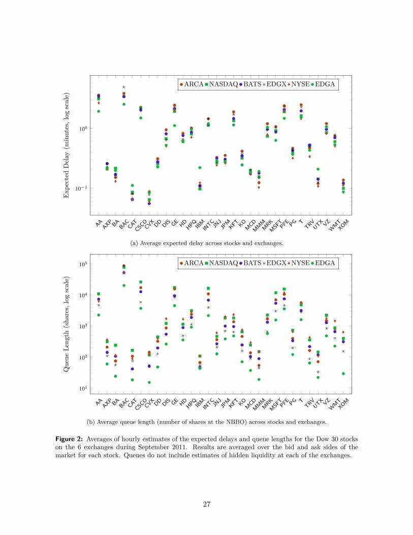
each stock and each exchange, Figure 2(a) shows the expected delay, averaged across time slots and

the bid and ask sides of the market. Delays range from 5 seconds to about 5 minutes across the 30

stocks we studied, and we observe 2x to 3x variation in the delay estimates at different exchanges

for the same security. Similarly, for each stock and each exchange, Figure 2(b) shows the average

queue lengths, or, the number of shares available at the NBBO, averaged across time slots and the

bid and ask sides of the market. Queue lengths range from 10 to 100,000 shares across securities,

and exhibit about a 10x variation in the queue sizes across exchanges for the same security. Deeper

queues correspond to longer delays.

Principle component analysis (PCA). The state space collapse result of our model predicts

that delays are coupled across exchanges and are restricted to a 1-dimensional subspace. Define the

empirically observed expected delay vector trajectories{

ED(s,j)(t) : t = 1, . . . , T ; s = BID,ASK},

where ED(s,j)(t) was estimated in (29) and the trajectories consider all one hour time slots in

the 21 days of our observation period. A natural way to test the effective dimensionality of this

vector of trajectories is via PCA by examining the number of principle components necessary to

explain the variability of the expected delay trajectories across exchanges and over time. The

output of the PCA analysis is summarized in Table 5: the first principle component explains15The time intervals should be sufficiently long so as to get reliable estimates of the event rates, and also long when

compared to the event inter-arrival times, so that one could expect that the transient dynamics of the market due tochanges in these rates settle down during these time intervals.

26

AAAXP BA

BACCAT

CSCOCVX DD DIS GE HD

HPQIB

MIN

TCJN

JJP

MKFT KO

MCDMMM

MRKMSF

TPFE PG T

TRVUTX VZ

WMT

XOM

10−1

100

Expe

cted

Del

ay(m

inut

es,l

ogsc

ale)

ARCA NASDAQ BATS EDGX NYSE EDGA

(a) Average expected delay across stocks and exchanges.

AAAXP BA

BACCAT

CSCOCVX DD DIS GE HD

HPQIB

MIN

TCJN

JJP

MKFT KO

MCDMMM

MRKMSF

TPFE PG T

TRVUTX VZ

WMT

XOM

101

102

103

104

105

Que

ueLe

ngth

(sha

res,

log

scal

e)

ARCA NASDAQ BATS EDGX NYSE EDGA

(b) Average queue length (number of shares at the NBBO) across stocks and exchanges.

Figure 2: Averages of hourly estimates of the expected delays and queue lengths for the Dow 30 stockson the 6 exchanges during September 2011. Results are averaged over the bid and ask sides of themarket for each stock. Queues do not include estimates of hidden liquidity at each of the exchanges.

27

% of Variance Explained % of Variance ExplainedOne Factor Two Factors One Factor Two Factors

Alcoa 80% 88% JPMorgan 90% 94%American Express 78% 88% Kraft 86% 92%

Boeing 81% 87% Coca-Cola 87% 93%Bank of America 85% 93% McDonalds 81% 89%

Caterpillar 71% 83% 3M 71% 81%Cisco 88% 93% Merck 83% 91%

Chevron 78% 87% Microsoft 87% 95%DuPont 86% 92% Pfizer 83% 89%Disney 87% 91% Procter & Gamble 85% 92%

General Electric 87% 94% AT&T 82% 89%Home Depot 89% 94% Travelers 80% 88%

Hewlett-Packard 87% 92% United Tech 75% 88%IBM 73% 84% Verizon 85% 91%Intel 89% 93% Wal-Mart 89% 93%

Johnson & Johnson 87% 91% Exxon Mobil 86% 92%

Table 5: Results of PCA: how much variance in the data can the first two principle components explain.

around 80% of the variability of the expected delays across exchanges, and the first two principle

components explain about 90%. This is consistent with the hypothesis of low effective dimen-

sion. In contrast, when we conduct PCA for the vector trajectories of observed queue lengths{Q(s,j)(t) : t = 1, . . . , T ; s = BID,ASK

}, we find relatively weaker evidence for a low effective di-

mensionality. In this test, the first principle component explains about 65% of the variability of

the queue lengths across exchanges, and the first two principle components explain less than 80%.

A detailed report of the results can be found in Table 17 in the Appendix.

Intuitively, in the high flow environment of our observation universe, i.e., where Λ and µ are

large, expected delay deviations from the equilibrium configuration would be quickly erased by

optimized arriving limit and market orders. The equilibrium state itself changes over time as the

rates of events change, but the coupling across exchanges remains strong, and persists even if we

shorten the time period over which market statistics are averaged from 1 hour down to 15 minutes.16

4.2. Estimation of the Market Order Routing Model

Define µ(s,j)i (t) to be the total arrival rate of market orders for security j and side s ∈ {BID,ASK}

in time slot t directed to exchange i, and let µ(s,j)(t) be the total arrival rate across all exchanges16For example, with 15 minute periods, the first principle component still explains 69% of the overall variability

of the vector of delay trajectories (that are themselves four times longer), while the first two principle componentsexplains 82% of the variability.

28

for (s, j) in time t. The attraction model of Section 2.2 for market orders suggests the relationship

(30) µ(s,j)i (t) = µ(s,j)(t) β

(j)i Q

(s,j)i∑N

i′=1 β(j)i′ Q

(s,j)i′

,

where β(j)i is the attraction coefficient for security j on exchange i. Note that our market order

routing model is invariant to scaling of the attraction coefficients, hence we normalize so that the

attraction coefficient for each stock on its listing exchange is 1. Given that {µ(s,j)i (t)}, {µ(s,j)(t)},

and {Q(s,j)i (t)} are observable, we estimated the β(j)

i ’s using a nonlinear regression on (30). The

results are given in Table 6. Note that all attraction coefficient estimates are statistically significant.

4.3. Empirical Evidence of State Space Collapse

Our model postulates the investors make order placement decisions by trading off delay against

effective rebates, and concludes that delays across exchanges, as measured by Q(s,j)i /µ

(s,j)i are

linearly related. It gives an expression for estimating delays in each exchange in terms of an

aggregate measure of market depth, which we call workload.

Verification of linear dependence of expected delays via regression analysis. Denote by

W (s,j)(t) the workload for side s of security j in time slot t, i.e.,

(31) W (s,j)(t) ,N∑i=1

β(j)i Q

(s,j)i (t),

and observe that using (30) the vector of expected delays can be written as

(32) ED(s,j)(t) = W (s,j)(t)µ(s,j)(t)

(1β

(j)1, . . . ,

1β

(j)N

).

In other words, the expected delays across different exchanges are linearly related, and specifically,

for each security j, exchanges i, i′, and market side s,

(33) ED(s,j)i (t) =

β(j)i′

β(j)i

ED(s,j)i′ (t),

for each time slot t. Testing the pairwise linear relations in (33) explores whether (ED1, . . . ,EDN )

live on a 1-dimensional space; this statistical test is based on the expected delay measurements

in (29), obtained by dividing the average observed queue size in each exchange with its respective

observed rate of trading, for all time slots, both sides of the market, and all the 30 component stocks

of the Dow Jones Industrial Average. For each stock and each exchange we have 126 measurements

29

Attraction CoefficientARCA NASDAQ BATS EDGX NYSE EDGA

Alcoa 0.73 0.87 0.76 0.81 1.00 1.33(0.01) (0.01) (0.01) (0.01) (0.00) (0.03)

American Express 1.19 1.08 0.99 0.94 1.00 0.94(0.02) (0.02) (0.04) (0.03) (0.00) (0.06)

Boeing 0.95 0.67 0.81 0.74 1.00 0.73(0.02) (0.01) (0.01) (0.02) (0.00) (0.04)

Bank of America 0.94 1.04 1.01 0.77 1.00 1.43(0.01) (0.02) (0.02) (0.01) (0.00) (0.04)

Caterpillar 0.82 0.78 1.13 0.70 1.00 0.58(0.01) (0.01) (0.03) (0.02) (0.00) (0.04)

Cisco 0.95 1.00 1.06 0.98 - 1.45(0.01) (0.00) (0.01) (0.02) - (0.03)

Chevron 0.70 0.93 1.17 0.65 1.00 0.75(0.01) (0.01) (0.02) (0.01) (0.00) (0.05)

DuPont 0.90 0.98 0.98 1.03 1.00 1.00(0.01) (0.01) (0.02) (0.02) (0.00) (0.06)

Disney 0.69 0.88 0.78 0.88 1.00 1.04(0.01) (0.01) (0.02) (0.03) (0.00) (0.03)

General Electric 0.79 1.01 0.94 0.73 1.00 1.63(0.01) (0.01) (0.02) (0.01) (0.00) (0.03)

Home Depot 0.76 0.98 0.79 0.84 1.00 1.02(0.01) (0.01) (0.01) (0.02) (0.00) (0.03)

Hewlett-Packard 1.04 1.04 1.02 0.68 1.00 0.82(0.02) (0.01) (0.02) (0.02) (0.00) (0.03)

IBM 1.25 1.20 1.20 1.05 1.00 0.54(0.02) (0.02) (0.03) (0.02) (0.00) (0.02)

Intel 0.83 1.00 0.96 0.84 - 1.04(0.01) (0.00) (0.01) (0.02) - (0.03)

Johnson & Johnson 0.80 0.94 0.86 0.92 1.00 0.77(0.01) (0.01) (0.01) (0.02) (0.00) (0.03)

JPMorgan 0.78 0.99 0.93 0.84 1.00 0.91(0.01) (0.01) (0.01) (0.01) (0.00) (0.02)

Kraft 0.72 0.89 0.83 0.73 1.00 1.06(0.01) (0.01) (0.01) (0.02) (0.00) (0.03)

Coca-Cola 0.68 0.84 0.79 0.76 1.00 0.88(0.01) (0.01) (0.02) (0.02) (0.00) (0.05)

McDonalds 0.90 0.86 1.03 0.82 1.00 0.82(0.01) (0.01) (0.02) (0.02) (0.00) (0.04)

3M 0.89 0.67 0.62 0.66 1.00 0.57(0.02) (0.01) (0.01) (0.02) (0.00) (0.04)

Merck 0.68 1.01 0.83 0.90 1.00 0.81(0.01) (0.01) (0.01) (0.02) (0.00) (0.02)

Microsoft 0.83 1.00 1.02 0.95 - 1.41(0.01) (0.00) (0.01) (0.02) - (0.03)

Pfizer 0.84 1.01 0.96 0.87 1.00 1.29(0.01) (0.01) (0.02) (0.02) (0.00) (0.03)

Procter & Gamble 0.79 0.89 0.88 0.89 1.00 0.89(0.01) (0.01) (0.01) (0.02) (0.00) (0.03)

AT&T 0.62 0.94 0.75 0.59 1.00 1.00(0.01) (0.01) (0.01) (0.01) (0.00) (0.03)

Travelers 0.80 0.69 0.69 0.84 1.00 0.80(0.01) (0.01) (0.01) (0.03) (0.00) (0.03)

United Tech 1.18 0.89 0.79 0.87 1.00 0.53(0.02) (0.01) (0.01) (0.03) (0.00) (0.04)

Verizon 0.77 0.95 0.88 0.72 1.00 0.85(0.01) (0.01) (0.01) (0.02) (0.00) (0.03)

Wal-Mart 0.72 0.88 0.79 0.71 1.00 0.91(0.01) (0.01) (0.01) (0.02) (0.00) (0.03)

Exxon Mobil 0.89 1.13 0.97 0.89 1.00 1.35(0.01) (0.01) (0.01) (0.02) (0.00) (0.10)

Table 6: Estimates of the attraction coefficients βi from nonlinear regression. Note that the attractioncoefficient of the listing exchange is normalized to be 1. We note that exchanges with lower fees (andrebates) tend to have higher attraction coefficients β.

30

in the respective time series per side of the market. The quality of the fit of these linear regressions

will be an indirect indication of the goodness of fit in (30). In more detail, we will perform a

cross-sectional regression. We will normalize the expected delay measurements at each exchange

by dividing them by the median expected delay of that security on a benchmark exchange (ARCA)

across all time slots and both sides of the market as follows

(34) ED(s,j)i (t) , ED(s,j)

i (t)median

τ=1,...,T ; s=BID,ASK

(ED(s,j)

ARCA(τ)) ,

where ED(s,j)i (t) was estimated in (29). We will perform a linear regression of the normalized left

side of (33), as a function of the normalized right side of (33), rescaled by the ratio of the attraction

coefficients of the two exchanges.

Dependent Variable: EDexchangeNASDAQ OMX BATS DirectEdge X NYSE DirectEdge A

Intercept 0.27∗∗∗ 0.28∗∗∗ 0.24∗∗∗ 0.28∗∗∗ 0.36∗∗∗(0.01) (0.01) (0.01) (0.01) (0.01)

Rescaled EDARCA 0.70∗∗∗ 0.72∗∗∗ 0.72∗∗∗ 0.63∗∗∗ 0.60∗∗∗(0.01) (0.01) (0.01) (0.01) (0.01)

R2 70% 70% 52% 60% 52%Note: ∗p < 0.1; ∗∗p < 0.05; ∗∗∗p < 0.01

Table 7: Linear regressions of the normalized expected delay on a particular exchange, versus that of thebenchmark exchange (ARCA) rescaled by the ratio of the attraction coefficients of the two exchanges.

The results of these regressions are summarized in Table 7. The R2 varies between 52% and

70% across the five exchanges. The results are statistically significant and we are able to reject

the null hypothesis that the delay on a particular exchange has a zero regression coefficient relative

to the rescaled delay on ARCA. These results statistically verify the linear dependence of delays

across different exchanges suggested by (33).

While the regressions in Table 7 were performed cross-sectionally across all securities, similar

results hold if the analysis is performed on a security by security basis. Figure 3 depicts the delay

relationships in the case of Bank of America. It illustrates the strong linear relationship across all

exchanges over time and across significant variations in prevailing market conditions; the latter is

manifested in the roughly two orders of magnitude variation in estimated expected delays.

A competing hypothesis is that queue lengths across exchanges are linearly related, that is, for

each security j, exchanges i, i′, and market side s,

(35) Q(s,j)i (t) = cii′Q

(s,j)i′ (t),

31

0 300 600 900 1,2000

300

600

900

1,200

rescaled ARCA delay (seconds)

NA

SDA

Qde

lay

(sec

onds

)

(a) slope = 0.88, intercept = 6× 10−3, R2 = 84%

0 300 600 900 1,2000

300

600

900

1,200

rescaled ARCA delay (seconds)

BAT

Sde

lay

(sec

onds

)

(b) slope = 0.80, intercept = 9× 10−3, R2 = 79%

0 300 600 900 1,2000

300

600

900

1,200

rescaled ARCA delay (seconds)

EDG

Xde

lay

(sec

onds

)

(c) slope = 1.04, intercept = 9× 10−4, R2 = 71%

0 300 600 900 1,2000

300

600

900

1,200

rescaled ARCA delay (seconds)

NY

SEde

lay

(sec

onds

)

(d) slope = 1.11, intercept = −4× 10−3, R2 = 63%

0 300 600 900 1,2000

300

600

900

1,200

rescaled ARCA delay (seconds)

EDG

Ade

lay

(sec

onds

)

(e) slope = 0.90, intercept = 4× 10−3, R2 = 73%

Figure 3: Scatter plots of the expected delay for Bank of America (BAC) on each exchange, versus thedelay on ARCA rescaled by the ratio of the attraction coefficients of the two exchanges. The black linescorrespond to linear regressions with intercept.

32

for each time slot t. The following test explores such an alternative hypothesis. According to (35),

predicated on queue length estimates obtained in Section 4.1, i.e., Q(s,j)i (t) as the average number

of shares available at the NBBO for time slot t, exchange i, stock j, and side s ∈ {BID,ASK},

we perform a cross-sectional linear regression of the queue length of each security on a particular

exchange, as a function of that on a benchmark exchange (ARCA). As before, we normalize the

queue lengths by dividing them by the median queue length of that security on a benchmark

exchange (ARCA) across all time slots and both sides of the market, i.e., we use

Q(s,j)i (t) , Q

(s,j)i (t)

medianτ=1,...,T ; s=BID,ASK

(Q

(s,j)ARCA(τ)

)as the queue length measure in the regression. Our model would predict that queue lengths will not

exhibit such a strong linear dependence as we show earlier in terms of delays. Indeed, the results

provided in Table 8 show that the R2 we found was significantly lower than that in Table 7, varying

between 13% and 26%.

Dependent Variable: QexchangeNASDAQ OMX BATS DirectEdge X NYSE DirectEdge A

Intercept 0.84∗∗∗ 0.39∗∗∗ 0.25∗∗∗ 0.57∗∗∗ 0.05∗∗∗(0.02) (0.01) (0.01) (0.02) (0.01)

QARCA 0.74∗∗∗ 0.45∗∗∗ 0.29∗∗∗ 0.96∗∗∗ 0.24∗∗∗(0.02) (0.01) (0.01) (0.02) (0.00)

R2 19% 20% 13% 26% 26%Note: ∗p < 0.1; ∗∗p < 0.05; ∗∗∗p < 0.01

Table 8: Linear regressions of the normalized queue length on a particular exchange versus that of thebenchmark exchange (ARCA).

Residual analysis and accuracy of delay estimates based on the aggregate workload. The

SSC result culminated in relationship (32) that makes expected delay predictions in each exchange

based on the 1-dimensional aggregated workload process. Specifically, given the market model

coefficients β(j)i and a measurement of the queue sizes at the various exchanges, Q(s,j)

i (t), one

can compute the workload via (31), and then construct estimates for the expected delays at the

various exchanges via (32). We denote the resulting delay estimates by ED(s,j)(t), where the ˆ

notation denotes in this context the estimate obtained via the one-dimensional workload process,

as opposed to measuring the actual expected delay ED(s,j)(t) via (29). This prediction can be

tested again through a set of linear regressions between the workload delay estimate and the delay

estimate that uses information about the state of the exchange (queue length and trading rate). All

these regressions are statistically significant and are accompanied with high R2 values. We do not

report on these results, instead we pursue a more detailed analysis of the residuals, i.e., the errors

33

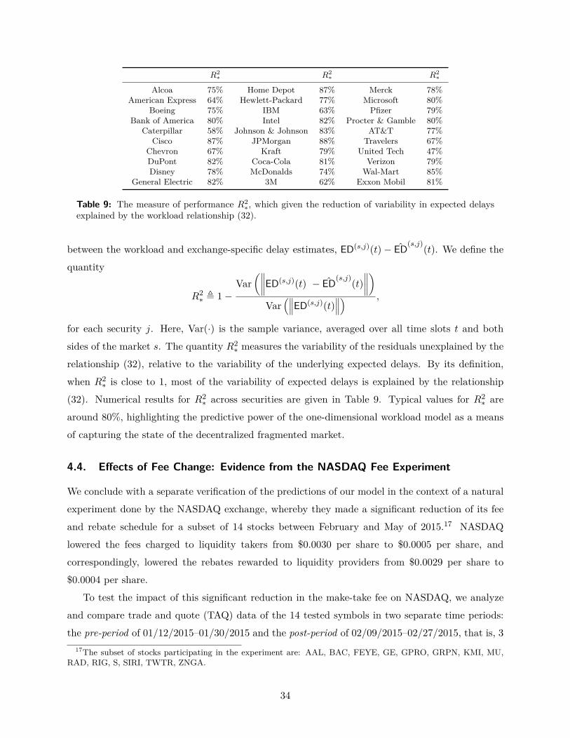
R2∗ R2

∗ R2∗

Alcoa 75% Home Depot 87% Merck 78%American Express 64% Hewlett-Packard 77% Microsoft 80%

Boeing 75% IBM 63% Pfizer 79%Bank of America 80% Intel 82% Procter & Gamble 80%

Caterpillar 58% Johnson & Johnson 83% AT&T 77%Cisco 87% JPMorgan 88% Travelers 67%

Chevron 67% Kraft 79% United Tech 47%DuPont 82% Coca-Cola 81% Verizon 79%Disney 78% McDonalds 74% Wal-Mart 85%

General Electric 82% 3M 62% Exxon Mobil 81%

Table 9: The measure of performance R2∗, which given the reduction of variability in expected delays

explained by the workload relationship (32).

between the workload and exchange-specific delay estimates, ED(s,j)(t)− ED(s,j)(t). We define the

quantity

R2∗ , 1−

Var(∥∥∥∥ED(s,j)(t) − ED(s,j)(t)

∥∥∥∥)Var

(∥∥∥ED(s,j)(t)∥∥∥) ,

for each security j. Here, Var(·) is the sample variance, averaged over all time slots t and both

sides of the market s. The quantity R2∗ measures the variability of the residuals unexplained by the

relationship (32), relative to the variability of the underlying expected delays. By its definition,

when R2∗ is close to 1, most of the variability of expected delays is explained by the relationship

(32). Numerical results for R2∗ across securities are given in Table 9. Typical values for R2

∗ are

around 80%, highlighting the predictive power of the one-dimensional workload model as a means

of capturing the state of the decentralized fragmented market.

4.4. Effects of Fee Change: Evidence from the NASDAQ Fee Experiment

We conclude with a separate verification of the predictions of our model in the context of a natural

experiment done by the NASDAQ exchange, whereby they made a significant reduction of its fee

and rebate schedule for a subset of 14 stocks between February and May of 2015.17 NASDAQ

lowered the fees charged to liquidity takers from $0.0030 per share to $0.0005 per share, and

correspondingly, lowered the rebates rewarded to liquidity providers from $0.0029 per share to

$0.0004 per share.

To test the impact of this significant reduction in the make-take fee on NASDAQ, we analyze

and compare trade and quote (TAQ) data of the 14 tested symbols in two separate time periods:

the pre-period of 01/12/2015–01/30/2015 and the post-period of 02/09/2015–02/27/2015, that is, 317The subset of stocks participating in the experiment are: AAL, BAC, FEYE, GE, GPRO, GRPN, KMI, MU,

RAD, RIG, S, SIRI, TWTR, ZNGA.

34

weeks before and after the initiation of the program at the beginning of February 2015, respectively.

Table 10 contains the fees charged on the 6 major exchanges in the tested periods, during which

only that of NASDAQ changed.

Exchange Fee($ per share, ×10−4)

NASDAQ OMX: January 2015 30.0February 2015 5.0

BATS 30.0DirectEdge X (EDGX) 30.0ARCA 30.0NYSE 27.0DirectEdge A (EDGA) -2.0

Table 10: Fees of the 6 major U.S. stock exchanges, per share traded, in January-February 2015 aroundthe time of the NASDAQ access fee experiment. Note that the fees here are different from previousfigures in table 4 because they are in different time periods.

A change in the per share fee and rebate will affect the attractiveness of the exchange for traders

placing limit orders and traders sending aggressive market orders. Our model of market and limit

order routing makes some direct predictions on market outcomes, specifically suggesting that the

fee change will affect both the trading rate and displayed depth at the exchange through their

impact on the expected delay experienced by limit orders.

In what follows, we will first estimate the exchange attraction coefficients before and after the fee

change. We will propose a structural model for the attractiveness of each exchange that explicitly

incorporates its prevailing fee. From this model, we expect that the attractiveness of NASDAQ is

increased after the fee reduction, and we verify this prediction. We then study the effect of the fee

change in the routing of limit orders. In this case, our model predicts that the equilibrium expected

delay for limit orders to get filled on NASDAQ will decrease after the fee change. The empirical

analysis will again verify this prediction.

Put together these observations suggest that the impact of the fee change is best understood

through its structural impact to limit and market order routing policies, and their impact on

trading delays. The agreement of our predictions with the observed market response suggests that

our model could be useful in addressing either policy related questions or questions of exchange

competition that often involves changes in pricing (fee/rebate) decisions. Our findings complement

those reported by Hatheway (2015a,b) and Pearson (2015) on the impact of this fee change; these

studies are not predicated on an underlying model of order routing, and primarily focused on market

share and depth comparisons, before and after the fee change.

Attraction coefficient βNASDAQ. The discussion in Section 2.2 suggested that the attrac-

tiveness of an exchange for market orders is a decreasing function of its fee. Our earlier analysis

35

focused on an observation period where fees were constant, which implied that the attractiveness

coefficients of the exchanges were themselves constant throughout that time period. The NASDAQ

fee experiment allows us to proceed with a more nuanced analysis to examine the effect of the

exchange fees on market order flow. We postulate the following structural model for the routing of

market orders:

(36) µ(s,j)i (t) = µ(s,j)(t)

[ea

(j)i +ri,tb(j)

]Q

(s,j)i (t)

∑Nk=1

[ea

(j)k

+rk,tb(j)]Q

(s,j)k (t)

.

In other words, we are postulating the attractiveness coefficients take the form β(j)i = ea

(j)i +ri,tb(j) ,

given parameters a(j)i , b(j) that we estimate using 3 weeks of data before and after the fee change.

Our hypothesis is that the parameter b(j) is negative, i.e., an higher fee makes an exchange less

desirable, all other things being equal. The corresponding {µ(s,j)i (t)}, {µ(s,j)(t)}, and {Q(s,j)

i (t)}

are estimated from the two trade and quote data samples as outlined in Section 4.1.

We normalize the results so that the parameter a(j)ARCA of the benchmark exchange ARCA is

0. Finally, b(j) is estimated using nonlinear regressions on (36), based on the combined sample for

each security. Results are in Table 11. Indeed, the estimated {b(j)} coefficients are negative for all

14 tested securities; 12 of these estimated coefficients are statistically significant at the 5% level of

the corresponding 1-sided test. This agrees with our hypothesis.

b(j) a(j)NASDAQ a

(j)EDGX a

(j)BATZ a

(j)NYSE a

(j)EDGA b NEGATIVE? 1-sided 5% test

AAL -4.92 0.11 -0.02 0.27 0.09 YES NOBAC -179.50 0.42 0.20 0.26 0.13 0.46 YES YESFEYE -98.65 -0.30 -0.20 0.10 -0.32 YES YESGE -93.50 0.15 -0.04 0.13 -0.01 0.27 YES YES

GPRO -50.15 -0.07 -0.21 0.07 -0.07 YES YESGRPN -94.41 0.12 -0.07 0.25 0.00 YES YESKMI -113.10 0.09 0.06 0.13 -0.18 -0.02 YES YESMU -89.02 0.06 -0.02 0.14 0.19 YES YESRAD -138.46 -0.05 -0.22 0.07 -0.29 -0.09 YES YESRIG -76.56 -0.02 -0.02 0.04 -0.14 0.10 YES YESS -162.59 -0.22 -0.29 0.04 -0.26 -0.38 YES YES

SIRI -69.31 0.13 -0.13 0.17 0.33 YES YESTWTR -87.33 -0.14 -0.16 -0.01 -0.27 -0.23 YES YESZNGA -17.66 0.14 -0.28 0.14 0.41 YES NO

Table 11: Estimates of b and ai in the attraction model (36) and hypothesis testing results on whetherthe coefficient b is negative. For each stock, the results are based on a combined sample that includesboth the pre-period and the post-period of the fee experiment.

We also directly estimate the βNASDAQ coefficients before and after the fee change and compare.

This estimation is non-parametric in the sense that it is not predicated on (36), and estimates

36

βNASDAQ via nonlinear regressions the following:

(37) µ(s,j)i (t) = µ(s,j)(t) β

(j)i Q

(s,j)i∑N

i′=1 β(j)i′ Q

(s,j)i′

,

based on the pre-period sample and the post-period sample, respectively. Our market order routing

model is invariant to scaling of the attraction coefficients and in this section we normalize so that

the attraction coefficient for each stock on the benchmark exchange ARCA is 1. Table 12 reports

and compares the estimated attraction coefficients before and after the NASDAQ fee experiment

for individual stocks. Note that β(j)NASDAQ - post is greater than β

(j)NASDAQ - pre for 12 out of the

14 tested securities. For all of these 12 names, the increments are statistically significant under a

1-sided test at the 5% level. This is again consistent with our prediction.

β(j)NASDAQ - pre Std. Dev. β

(j)NASDAQ - post Std. Dev. INCREASE? 1-sided 5% test

AAL 1.1478 0.0152 1.0787 0.0189 NO NOBAC 1.4516 0.0297 2.5617 0.0647 YES YESFEYE 0.6958 0.0136 0.9543 0.0156 YES YESGE 1.1339 0.0244 1.5250 0.0386 YES YES

GPRO 0.9285 0.0196 1.0557 0.0250 YES YESGRPN 1.1035 0.0253 1.4288 0.0258 YES YESKMI 1.0814 0.0163 1.4780 0.0267 YES YESMU 1.0314 0.0124 1.3862 0.0186 YES YESRAD 0.9515 0.0302 1.3530 0.0368 YES YESRIG 0.9775 0.0230 1.1925 0.0239 YES YESS 0.9905 0.0453 1.0957 0.0429 YES YES

SIRI 1.1787 0.0265 1.3045 0.0347 YES YESTWTR 0.9093 0.0235 1.0623 0.0269 YES YESZNGA 1.2111 0.0337 1.1939 0.0332 NO NO

Table 12: Estimates of the attraction coefficient of individual stocks on NASDAQ before and after thefee experiment, and hypothesis testing results on whether the attraction coefficient increases under thefee change.

Expected delay EDNASDAQ. Our limit order routing model suggests that traders tradeoff

expected delay with rebate, and that in equilibrium, exchanges that offer lower rebates will also

offer lower expected delays for limit orders placed in the back of the queue at the best bid (top of

book) until they get filled.

As stated in (12), the expected delay satisfies EDi = Wµβi

. We expect the workload W to remain

the same after NASDAQ reduces its make-take fee, as the equilibrium value of W depends on the

“marginal” exchange, which is likely to be the one with the lowest rebate, which is not NASDAQ;

we are assuming that the remaining model parameters remain the same. As described above, we

anticipate the attraction coefficient βNASDAQ to increase after the fee change, which would result

in a lower expected delay EDNASDAQ after NASDAQ reduced its make-take fee. An alternative

37

justification is that traders submitting orders into NASDAQ would expect lower expected delays

given that they are compensated with a lower rebate when their orders trade. In equilibrium, patient

traders will submit orders to higher rebate exchanges, which would result in a lower equilibrium

delay at NASDAQ after the fee change.

To test this hypothesis we will compare the normalized expected delay at NASDAQ before and

after the fee change. We first compute the measure of expected delay along the lines of Section 4.1,

as

(38) ED(s,j)i (t) , Q

(s,j)i (t)

µ(s,j)i (t)

,

for side s, security j, on exchange i, in time slot t. We then use these measures to calculate an

aggregate, normalized estimate of the expected delay on NASDAQ, as follows:

(39) ED(j)NASDAQ = 1

2T∑

s∈{BID,ASK}

T∑t=1

ED(s,j)NASDAQ(t)∑N

k=1 ED(s,j)k (t)

.

For each stock, we can obtain two estimates ED(j)NASDAQ - pre and ED(j)

NASDAQ - post based on the

pre-period sample and the post-period sample, respectively. Table 13 reports on these two statistics

for individual securities. We observe that the normalized expected delay on NASDAQ decreases

for all 14 tested securities; in 13 of these 14 cases, the reduction is statistically significant. This

agrees with the prediction of our model.

ED(j)NASDAQ - pre Std. Err. ED(j)

NASDAQ - post Std. Err. DECREASE? 1-sided 5% test

AAL 0.1978 0.0023 0.1886 0.0027 YES YESBAC 0.1556 0.0022 0.0963 0.0020 YES YESFEYE 0.2282 0.0037 0.1964 0.0031 YES YESGE 0.1688 0.0026 0.1265 0.0023 YES YES

GPRO 0.2262 0.0053 0.2145 0.0057 YES NOGRPN 0.2030 0.0034 0.1700 0.0035 YES YESKMI 0.1646 0.0018 0.1265 0.0018 YES YESMU 0.2062 0.0023 0.1683 0.0024 YES YESRAD 0.1750 0.0038 0.1027 0.0030 YES YESRIG 0.1721 0.0022 0.1401 0.0024 YES YESS 0.1765 0.0063 0.1305 0.0034 YES YES

SIRI 0.2150 0.0072 0.1558 0.0077 YES YESTWTR 0.1813 0.0026 0.1453 0.0035 YES YESZNGA 0.1831 0.0062 0.1515 0.0054 YES YES

Table 13: Estimates of the normalized expected delay on NASDAQ of individual stocks before and afterthe fee experiment, and hypothesis testing results on whether the normalized expected delay decreasesunder the fee change.

Linear relation EDNASDAQ = βARCA/βNASDAQ · EDARCA. Last we examine how the

38

ED(j)NASDAQ - pre Std. Err. ED(j)

NASDAQ - post Std. Err. DECREASE? 1-sided 5% test

AAL 1.0029 0.0109 0.9681 0.0139 YES YESBAC 0.9293 0.0121 0.5895 0.0137 YES YESFEYE 1.2431 0.0202 1.0567 0.0164 YES YESGE 1.0267 0.0160 0.7863 0.0169 YES YES

GPRO 1.1619 0.0336 1.0842 0.0360 YES NOGRPN 1.0468 0.0191 0.8941 0.0168 YES YESKMI 0.9938 0.0100 0.7622 0.0108 YES YESMU 1.0318 0.0114 0.8699 0.0127 YES YESRAD 1.1165 0.0303 0.6757 0.0195 YES YESRIG 1.0361 0.0128 0.8614 0.0142 YES YESS 1.2665 0.0711 0.8699 0.0218 YES YES

SIRI 1.4101 0.1685 1.4559 0.4852 NO NOTWTR 1.1077 0.0166 0.9034 0.0260 YES YESZNGA 1.0337 0.0404 0.8984 0.0308 YES YES

Table 14: Results in parallel to those in Table 13 when the expected delays are normalized by mediandelay instead of by sum of delays.

fee change affects the linear relation (33) in Section 4.3, which is one of the major conclusions

arising from our model,

(40) ED(s,j)i (t) =

β(j)i′

β(j)i

ED(s,j)i′ (t).

Specially, we want to test that when considering the above linear relation between NASDAQ and

the benchmark exchange, ARCA, the slope of that linear relation before and after the fee change

will decrease, since we expect that the attraction coefficient βNASDAQ should increase in response

to that change. We perform linear regressions for each security between the expected delays on

NASDAQ against that on the benchmark exchange ARCA before and after the fee change and report

the results in Table 15. We observe that the resulting slopes decrease for all 14 tested securities,

among which 8 are statistically significant under a one-sided test at the 5% level. In addition, in a

cross-sectional linear regression the slope before the fee change was 0.78564∗∗∗(0.01571), R2 = 58%,

and 0.66384∗∗∗(0.01221), R2 = 62% after the fee change; the decrease in the slope is statistically

significant.

References

A. Alfonsi, A. Fruth, and A. Schied. Optimal execution strategies in limit order books with generalshape functions. Quantitative Finance, 10:143–157, 2010.

G. Allon and A. Federgruen. Competition in service industries. Operations Research, 55(1):37–55,2007.

39

slope (before) Std. Err. slope (after) Std. Err. DECREASE? 1-sided 5% test

AAL 0.6742 0.0308 0.5981 0.0392 YES NOBAC 0.6176 0.0299 0.3245 0.0269 YES YESFEYE 0.8773 0.0761 0.7950 0.0543 YES NOGE 0.7851 0.0384 0.4859 0.0349 YES YES

GPRO 0.3744 0.0458 0.3314 0.0624 YES NOGRPN 0.9570 0.0418 0.8223 0.0234 YES YESKMI 0.8764 0.0289 0.5400 0.0255 YES YESMU 0.8313 0.0277 0.5741 0.0274 YES YESRAD 0.9439 0.0611 0.3090 0.0482 YES YESRIG 0.6571 0.0286 0.5360 0.0282 YES YESS 0.5740 0.1151 0.5406 0.0395 YES NO

SIRI 1.3337 0.2686 (0.0001) 0.0135 YES YESTWTR 0.8406 0.0679 0.7470 0.0724 YES NOZNGA 0.0546 0.0087 0.0425 0.0174 YES NO

Table 15: Linear regression results of equation (40) and hypothesis testing results on whether the slopedecreases after the fee change on NASDAQ.

slope (before) Std. Err. slope (after) Std. Err. DECREASE? 1-sided 5% test

AAL 0.7960 0.0149 0.8121 0.0188 NO NOBAC 0.6774 0.0154 0.3789 0.0138 YES YESFEYE 1.3292 0.0428 1.0828 0.0288 YES YESGE 0.8285 0.0221 0.5942 0.0194 YES YES

GPRO 0.7147 0.0375 0.6852 0.0453 YES NOGRPN 0.9706 0.0294 0.8040 0.0207 YES YESKMI 0.9253 0.0150 0.6436 0.0123 YES YESMU 0.9034 0.0152 0.6440 0.0140 YES YESRAD 1.0516 0.0440 0.4285 0.0366 YES YESRIG 0.7851 0.0199 0.6453 0.0177 YES YESS 0.6519 0.1113 0.6650 0.0299 NO NO

SIRI 1.4071 0.2435 0.0017 0.0134 YES YESTWTR 1.1070 0.0354 0.8970 0.0390 YES YESZNGA 0.0584 0.0091 0.0550 0.0178 YES NO

Table 16: Results in parallel to those in Table 15 when the linear regressions are performed withoutintercept.

M. J. Barclay, T. Hendershott, and T. D. McCormick. Competition among trading venues: Infor-mation and trading on electronic communications networks. Journal of Finance, 58:2637–2666,2003.

A. Bassamboo, J.M. Harrison, and A. Zeevi. Dynamic routing in large call centers: Asymptoticanalysis of an LP-based method. Operations Research, 10:1074–1099, 2004.

O. Besbes and C. Maglaras. Revenue optimization for a make-to-order queue in an uncertain marketenvironment. Operations Research, 57(6):1438–1450, 2009.

H. Bessembinder. Quote-based competition and trade execution costs in NYSE listed stocks. Jour-nal of Financial Economics, 70:385–422, 2003.

40

B. Biais, C. Bisière, and C. Spatt. Imperfect competition in financial markets: An empirical studyof Island and Nasdaq. Management Science, 56(12):2237–2250, 2010.

J. Blanchet and X. Chen. Continuous-time modeling of bid-ask spread and price dynamics in limitorder books. Working paper, 2013.

J.-P. Bouchaud, Y. Gefen, M. Potters, and M. Wyart. Fluctuations and response in financialmarkets: The subtle nature of ‘random’ price changes. Quantitative Finance, 4:176–190, 2004.

M. Bramson. State space collapse with applications to heavy-traffic limits for multiclass queueingnetworks. QUESTA, 30:89–148, 1998.

S. Buti, B. Rindi, Y. Wen, and I.M. Werner. Tick size regulation, intermarket competition andsub&penny trading. Working paper, 2011.

G. Cachon and P. Harker. Competition and outsourcing with scale economies. Management Science,48:1314–1333, 2002.

R. Caldentey, E. Kaplan, and G. Weiss. Fcfs infinite bipartite matching of servers and customers.Adv. of Applied Probability, 41(3):695–730, 2009.

Y-J. Chen, C. Maglaras, and G. Vulcano. Design of an aggregated marketplace under congestioneffects: Asymptotic analysis and equilibrium characterization. Working paper, 2010.

R. Cont and A. Kukanov. Optimal order placement in limit order markets. Working paper, 2013.

R. Cont and A. De Larrard. Price dynamics in a markovian limit order market. SIAM Journal ofFinancial Mathematics, 4(1):1–25, 2013.

R. Cont, S. Stoikov, and R. Talreja. A stochastic model for order book dynamics. OperationsResearch, 58:549–563, 2010.

H. Degryse, F. de Jong, and V. van Kervel. The impact of dark trading and visible fragmentationon market quality. Working paper, 2011.

A. Dufour and R. F. Engle. Time and the price impact of a trade. Journal of Finance, 55:2467–2498,2000.

T. Foucault and A. J. Menkveld. Competition for order flow and smart order routing systems.Journal of Finance, 63:119–158, 2008.

T. Foucault, O. Kadan, and E. Kandel. Limit order book as a market for liquidity. Review ofFinancial Studies, 18:1171–1217, 2005.

41

J. Gatheral. No-dynamic-arbitrage and market impact. Quantitative Finance, 10:749–759, 2010.

L. Glosten. Is the electronic order book inevitable? Journal of Finance, 49:1127–1161, 1994.

L. Glosten. Competition, design of exchanges and welfare. Working paper, 1998.

L. R. Glosten. Components of the bid/ask spread and the statistical properties of transactionprices. Journal of Finance, 42:1293–1307, 1987.

L. R. Glosten and P. R. Milgrom. Bid, ask, and transaction prices in a specialist market withheterogeneously informed traders. Journal of Financial Economics, 14:71–100, 1985.

M. D. Griffiths, B. F. Smith, D. A. S. Turnbull, and R. W. White. The costs and the determinantsof order aggressiveness. Journal of Financial Economics, 56:65–88, 2000.

X. Guo, A. De Larrard, and Z. Ruan. Optimal placement in a limit order book. Working paper,2013.

I. Gurvich and A. Ward. On the dynamic control of matching queues. Stochastic Systems, 4(2):479–523, 2014.

J. L. Hamilton. Marketplace fragmentation, competition, and the efficiency of the stock exchange.Journal of Finance, 34:171–187, 1979.

J. M. Harrison. Brownian models of queueing networks with heterogeneous customer populations.In W. Fleming and P. L. Lions, editors, Stochastic Differential Systems, Stochastic Control Theoryand Applications, volume 10 of Proceedings of the IMA, pages 147–186. Springer-Verlag, New York,1988.

J. M. Harrison. Balanced fluid models of multiclass queueing networks: a heavy traffic conjecture.In F. Kelly and R. Williams, editors, Stochastic Networks, volume 71, pages 1–20. Proceedings ofthe IMA, 1995.

J. M. Harrison. Brownian models of open processing networks: Canonical representation of work-load. Ann. Appl. Prob., 10:75–103, 2000.

J. M. Harrison and M. J. Lopez. Heavy traffic resource pooling in parallel- server systems. QueueingSystems, 33:339–368, 1999.

R. Hassin and M. Haviv. To Queue or not to Queue: Equilibrium Behavior in Queueing Systems.Kluwer Academic Publishers, Boston, MA, 2003.

F. Hatheway. Nasdaq access fee experiment. Nasdaq, Technical report, 2015a.

42

F. Hatheway. Nasdaq access fee experiment. Nasdaq, Technical report, 2015b.

B. Hollifield, R. A. Millerz, and P. Sandas. Empirical analysis of limit order markets. Review ofEconomic Studies, 71:1027–1063, 2004.

R. W. Holthausen, R. W. Leftwich, and D. Mayers. Large-block transactions, the speed of response,and temporary and permanent stock-price effects. Journal of Financial Economics, 26:71–95,1990.

G. Huberman and W. Stanzl. Price manipulation and quasi-arbitrage. Econometrica, 72:1247–1275,2004.

B. Jovanovic and A. J. Menkveld. Middlemen in limit-order markets. Working paper, 2011.

D. B. Keim and A. Madhavan. The cost of instituional equity trades. Financial Analysts Journal,54:50–59, 1998.

A. Kukanov and C. Maglaras. A limit order queue model with traders with heterogeneous behaviors.Working paper, Columbia University, 2015.

Thomas G. Kurtz. Strong approximation theorems for density dependent Markov chains. StochasticProcesses Appl., 6(3):223–240, 1977/78. ISSN 0304-4149.

A. S. Kyle. Continuous auctions and insider trading. Econometrica, 53:1315–1335, 1985.

P. Lakner, J. Reed, and S. Stoikov. High frequency asymptotics for the limit order book. Workingpaper, 2013.

P. Lakner, J. Reed, and F. Simatos. Scaling limit of a limit order book model via the regenerativecharacterization of lévy trees. Working paper, 2014.

M. A Lariviere. A note on probability distributions with increasing generalized failure rates. Op-erations Research, 54(3):602–604, 2006.

P. Lederer and L. Li. Pricing, production, scheduling and delivery -time competition. OperationsResearch, 45:407–420, 1997.

D. Levhari and I. Luski. Duopoly prcing and waiting lines. European Economic Review, 11:17–35,1978.

L. Li and Y. Lee. Pricing and delivery-time performance in a competitive environment. ManagementScience, 40:633–646, 1994.

43

I. Luski. On partial equilibrium in a queueing system with two servers. The Review of EconomicStudies, 43:519–525, 1976.

C. Maglaras, C. Moallemi, and H. Zheng. Optimal execution in a limit order book and an associatedmicrostructure market impact model. Working paper, 2014.

K. Malinova and A. Park. Liquidity, volume, and price behavior: The impact of order vs. quotebased trading. Working paper, 2010.

A. Mandelbaum and G. Pats. State-dependent queues: approximations and applications. In F. Kellyand R. Williams, editors, Stochastic Networks, volume 71, pages 239–282. Proceedings of the IMA,1995.

H. Mendelson and S. Whang. Optimal incentive-compatible priority pricing for the m/m/1 queue.Oper. Res., 38(5):870–883, 1990.

A. Obizhaeva and J. Wang. Optimal trading strategy and supply/demand dynamics. Workingpaper, 2006.

M. O’Hara and M. Ye. Is market fragmentation harming market quality? Journal of FinancialEconomics, 100(3):459–474, June 2011.

C. Parlour. Limit order markets: A survey. Handbook of Financial Intermediation & BankingA.W.A. Boot and A. V. Thakor eds., 2008.

C. A. Parlour. Price dynamics in limit order markets. Review of Financial Studies, 11:789–816,1998.

P. Pearson. Takeways from the NASDAQ pilor program. ITG Technical Report, 2015.

E. L. Plambeck and A. R. Ward. Optimal control of a high-volume assemble-to-order system. Math.Oper. Res., 31(3):453–477, 2006.

I. Rosu. A dynamic model of the limit order book. Review of Financial Studies, 22:4601–4641,2009.

K. So. Price and time competition for service delivery. Manufacturing & Service OperationsManagement, 2(4):392–409, 2000.

G. Sofianos. Specialist gross trading revenues at the New York Stock Exchange. Working paper,1995.

44

G. Sofianos, J. Xiang, and A. Yousefi. Smart order routing: All-in shortfall and optimal orderplacement. Goldman Sachs, Equity Executions Strats, Street Smart, 42, 2011.

S. Stoikov, M. Avellaneda, and J. Reed. Forecasting prices from level-i quotes in the presence ofhidden liquidity. Algorithmic Finance, Forthcoming, 2011.

A. L. Stolyar. Optimal routing in output-queued flexible server systems. Probability in the Engi-neering and Informational Sciences, 19:141 – 189, 2005.

V. van Kervel. Liquidity: What you see is what you get? Working paper, 2012.

S. H. Zak. Systems and Control. Oxford University Press, 2003.

A. Proofs: Equilibrium Characterization

Proof of Lemma 1. For γ ≥ 0, define L(γ) , maxi 6=0 γ(ri − r0) − W ∗

µβi. Clearly L is a continuous

function, and under Assumption 1(iii), it is also increasing. We wish to show that L(γ0) = 0.

Suppose that L(γ0) < 0. Then, there exists γ > γ0 with L(γ) < 0 for all γ ∈ [0, γ]. Thus, in

equilibrium, investors with types γ ∈ [0, γ] strictly prefer placing market orders, i.e., π∗i (γ) = 0 for

i 6= 0. Then,

N∑i=1

(λi + Λ

∫ ∞0

π∗i (γ) dF (γ))

=N∑i=1

λi + Λ∫ ∞γ0

(N∑i=1

π∗i (γ))dF (γ) ≤

N∑i=1

λi + Λ(1− F (γ)

)< µ,

where the last inequality follows from (17) and Assumption 1(i). This contradicts the flow balance

equation (14).

Alternatively, suppose that L(γ0) > 0. Then, there exists γ < γ0 with L(γ) > 0 for all

γ ∈ [γ,∞). Thus, in equilibrium, investors with types γ ∈ [γ,∞) strictly prefer not placing market

orders, i.e., π∗0(γ) = 0. Then,

N∑i=1

(λi + Λ

∫ ∞0

π∗i (γ) dF (γ))

=N∑i=1

λi + Λ∫ ∞

0(1− π∗0(γ)) dF (γ)

≥N∑i=1

λi + Λ(1− F (γ)

)> µ,

where the last inequality follows from (17) and Assumption 1(i). This contradicts the flow balance

equation (14). Thus, we must have L(γ0) = 0 and (20) holds.

45

Now, suppose exchange i achieves the maximum in (20). Then, from the right side of (20), it

follows that κi = βi(ri− r0) = W ∗

µγ0. Further, for any exchange j, (20) implies that κj = βj(rj− r0) ≤

W ∗

µγ0= κi. For the converse, if

(A.1) κi = maxj 6=0

κj ,

and there exists an exchange j satisfying

0 = γ0(rj − r0)− W ∗

µβj> γ0(ri − r0)− W ∗

µβi,

then

κj = βj(rj − r0) = W ∗

µγ0> βi(ri − r0) = κi,

which contradicts with (A.1). �

Proof of Theorem 2. Suppose (π∗,W ∗) satisfies (22)–(23). We want to show that (π∗,W ∗) is an

equilibrium, i.e., it must satisfy (13)–(14).

We first establish (13). In particular, we will establish that for any π ∈ P and all γ,

π0(γ)γr0 +N∑i=1

πi(γ)(γri −

W ∗

µβi

)≤ π∗0(γ)γr0 +

N∑i=1

π∗i (γ)(γri −

W ∗

µβi

).

Equivalently,

(A.2)N∑i=1

πi(γ)(γ (ri − r0)− W ∗

µβi

)≤

N∑i=1

π∗i (γ)(γ (ri − r0)− W ∗

µβi

).

If γ ≤ γ0 and i 6= 0, using (22) and Assumption 1(iii), we have that

γ (ri − r0)− W ∗

µβi= γκi − γ0 maxj 6=0 κj

βi≤ γ0κi − γ0 maxj 6=0 κj

βi≤ 0(A.3)

Since, by (23), π∗i (γ) = 0 for i 6= 0, we have that (A.2) holds for all γ < γ0. For γ = γ0, note

that equality holds in (A.3) iff κi = maxj 6=0 κj , i.e., i ∈ A∗(γ0). Thus, (A.2) also holds for γ = γ0.

Finally, if γ > γ0 and i 6= 0,

(A.4) γ (ri − r0)− W ∗

µβi= γκi − γ0 maxj 6=0 κj

βi≥ γκi − γmaxj 6=0 κj

βi≥ 0.

Thus, (A.2) continues to hold.

46

Next, we establish (14). By (23), 1− π∗0(γ) = 0 when γ < γ0 and 1− π∗0(γ) = 1 when γ > γ0.

Thus, ∫ ∞0

(1− π∗0(γ)

)dF (γ) =

∫ ∞γ0

dF (γ) = 1− F (γ0).

Using this and (17),

µ =N∑i=1

λi + Λ∫ ∞

0

(1− π∗0(γ)

)dF (γ)

=N∑i=1

λi + Λ∫ ∞

0

(N∑i=1

π∗i (γ))dF (γ)

=N∑i=1

(λi + Λ

∫ ∞0

π∗i (γ) dF (γ)).

Thus, (π∗,W ∗) satisfies (14) as well and is an equilibrium.

Now suppose (π∗,W ∗) is an equilibrium. We would like to show that (π∗,W ∗) must satisfy

(22)–(23), except possibly for γ in a set of F -measure zero.

First, by Lemma 1, we have that

γ0r0 = maxi 6=0

γ0ri −W ∗

µβi= γ0ri −

W ∗

µβi,

where i ∈ argmaxj 6=0 κj . By solving for W ∗, (22) follows immediately.

Next, we verify (23). Define M to be the set of γ ≥ 0 such that π∗(γ) does not satisfy (23).

Define π ∈ P to be a set of routing decisions such that (π,W ∗) satisfies (23), such a π can easily

be constructed by solving the optimization problem for A∗(γ) for each γ ≥ 0. Define

∆(γ) , π∗0(γ)r0 +N∑i=1

π∗i (γ)(γri −

W ∗

µβi

)− π0(γ)r0 −

N∑i=1

πi(γ)(γri −

W ∗

µβi

)

=N∑i=1

π∗i (γ)(γ (ri − r0)− W ∗

µβi

)−

N∑i=1

πi(γ)(γ (ri − r0)− W ∗

µβi

),

for γ ≥ 0. Following the same arguments as in (A.3)–(A.4), it is easy to see that

(A.5)∆(γ) = 0 if γ /∈M,

∆(γ)< 0 if γ ∈M and γ 6= γ0.

47

On the other hand, Since π∗ is optimal for the program (13), we have that

(A.6) 0 ≤∫ ∞

0∆(γ) dF (γ) =

∫M

∆(γ) dF (γ) =∫M∩[0,γ0)

∆(γ) dF (γ) +∫M∩(γ0,∞)

∆(γ) dF (γ),

where, for the final equality, we use the fact that the point {γ0} has F -measure zero under As-

sumption 1(i). Together, (A.5)–(A.6) imply thatM has F -measure 0. �

B. Proofs: Equilibrium Convergence

In this appendix, we prove the convergence of the queue length process Q(t) to the unique equilib-

rium vector Q∗ at t→∞, in the two-dimensional case.

We first provide the proof of Theorem 3, which establishes uniqueness of the equilibrium queue

length vector Q∗.

Proof of Theorem 3. Suppose(π(1), Q(1)) and

(π(2), Q(2)) are both equilibria. Define W (`) ,

β>Q(`), for ` ∈ {1, 2}. By Theorem 1, both(π(1),W (1)) and

(π(2),W (2)) satisfy (13)-(14). By

Theorem 2, we have that

(B.1) W (1) = W (2) = W ∗ , γ0µmaxi 6=0

κi.

Now, suppose that γ < γ0. Theorem 2 states that π(1)i (γ) = π

(2)i (γ) = 0 for i 6= 0, except

possibly on a set of γ of F -measure zero. On the other hand, if γ > γ0, by Theorem 2, π(1)(γ) and

π(2)(γ) can only differ when A∗(γ) contains at least two exchanges (ignoring a set of γ of at most

F -measure zero). Suppose {i, j} are two exchanges such that {i, j} ⊂ A∗(γ), i.e., a type-γ investor

is indifferent between exchanges i and j. Then,

(B.2) γ(ri − rj) = W ∗

µβi− W ∗

µβj.

The right hand side of (B.2) is independent of γ, and ri − rj 6= 0, by the assumption that the

effective rebates are distinct. Then, {i, j} ⊂ A∗(γ) for at most a single value of γ. As there are

only finitely many pairs of exchanges, we have that |A∗(γ)| = 1 except for possibly finitely many

γ > γ0. Then, under Assumption 1(i), π(1)(γ) and π(2)(γ) differ on a set of γ of at most F -measure

zero.

48

Combining these facts with the flow balance condition (11), we have that

Q(1)i = Q

(1)i ×

µβiµβi× W ∗

β>Q(1) = µi(Q(1))W ∗

µβi

=(λi + Λ

∫ ∞0

π(1)i (γ) dF (γ)

)W ∗

µβi

=(λi + Λ

∫ ∞0

π(2)i (γ) dF (γ)

)W ∗

µβi

= Q(2)i ,

for i = 1, . . . , N , i.e., the equilibrium queue lengths are unique. �

Next we prove the convergence of the queue length process Q(t) to the unique equilibrium vector

Q∗ at t→∞, in the two-dimensional case.

As in Section 2.3, define χi(W (t)) to be the instantaneous fraction of arriving limit orders that

are placed into exchange i. The evolution of the queue length process Q(t) is characterized by the

following system of ordinary differential equations,

(B.3) Qi(t) = λi + Λχi(W (t))− µi(Q(t)), i = 1, . . . , N.

In the remainder of this appendix, we focus on the two dimensional cases, i.e., N = 2. Also, without

loss of generality, we assume λi = 0, for i = 1, 2.18

The fact that the equilibrium queue length vector exhibits state space collapse and leads us

to consider a new coordinate system in which workload W , β>Q is one of the new coordinates.

In the two dimensional case, the workload W together with the sum of queue lengths S , 1>Q

characterize the individual queue lengths and vice versa. Thus, the convergence of (W (t), S(t))

to (W ∗, S∗) where W ∗ , β>Q∗ and S∗ , 1>Q∗, is equivalent to the convergence of the queue

length process Q(t) to the unique equilibrium vector Q∗. We perform the change of coordinates

and rewrite the original ordinary differential equations in terms of W and S as follows:

(B.4)

W (t) = Λβ>χ(W (t))− µ(β1 + β2) · I{W (t) 6=0} + µ

β1β2S(t)W (t) · I{W (t)6=0},

˙S(t) = Λ1>χ(W (t))− µ · I{S(t)6=0}.

We will restrict attention to this new (W,S) coordinate system for the remainder of this appendix.18The proof that follows can be easily adapted to all other cases where λ1, λ2 > 0 and, λ1 + λ2 < µ.

49

B.1. Overview of the Proof for (W (t), S(t)) Convergence

In the following we prove that under Assumptions 1–3, given arbitrary initial conditions (W (0), S(0)) ∈

R2+, the process (W (t), S(t)) converges to the unique equilibrium (W ∗, S∗) at t→∞.

Define the set W+ , {(W,S) : W = W ∗, S > S∗}, i.e., the upper half of the vertical line

W = W ∗ in R2. We will show that (W (t), S(t)) either hits the set W+ or enters a local stability

region within a finite time, starting from any initial point. This will imply that (W (t), S(t))

returns to set W+ with finite inter-arrival times, if it has not entered the local stability region.

Each recurrence corresponds to a point on the upper half of the vertical line W = W ∗ in R2, i.e.,

to a value of S ≥ S∗. We then show that each recurrence has a smaller (closer to S∗) S value than

the previous appearance in set W+. Moreover, the step size is bounded away from zero as long

as the trajectory is outside the local stability region. This ensures there are finite iterations until

(W (t), S(t)) enters the local stability region, and thus has to converge.

Accordingly, the proof will be organized around the following main steps, each of which corre-

sponds to one of Lemmas 3-5 in the following subsection:

1. Lemma 3 (Local Stability). There exists ε > 0, such that if (W (0), S(0)) is in the set

Wlocal , {(W,S) : |W −W ∗| < ε, |S − S∗| < ε},

then (W (t), S(t)) converges to (W ∗, S∗).

2. Lemma 4 (Finite Inter-arrival Time). Starting from any initial point, a sample path either

enters the local stability region Wlocal or hits the set W+ in finite time; in the latter case,

starting from any point in W+ the sample path must, in finite time, either

(i) reach the set Wlocal,

(ii) return to the set W+.

3. Lemma 5 (Guaranteed Decay). There exists ϕ > 0, such that if τ1 < τ2 are times where

(W (τ1), S(τ1)), (W (τ2), S(τ2)) ∈W+ and (W (t), S(t)) 6∈Wlocal for t ∈ [τ1, τ2],

then S(τ2) ≤ S(τ1)− ϕ.

This method of proving (W (t), S(t)) convergence shows that each sample path is a decaying

spiral in R2 centered around the unique equilibrium point (W ∗, S∗). Analyzing the spiral, we show

50

that each rotation takes finite time, and has a guaranteed decay towards the equilibrium along the

S coordinate at times when the set W+ is hit.

Therefore, the spiral enters the local stability region after finite iterations and within finite time,

at which point it much converge to the unique equilibrium.

B.2. Proving (W (t), S(t)) Convergence

We begin with a lemma that provides a series of bounds on the trajectory. First, we postulate that

(W (t), S(t)) should be within the first quadrant R2+, since both components are positive weighted

sum of the queue lengths. Second, the ratio S(t)/W (t) is bounded by the largest and smallest of

{1/βi}i=1,2. Recall that we assume attraction coefficients are distinct. Without loss of generality,

assume that β1 > β2 and define C , {(W,S) : S/W ∈ [1/β1, 1/β2]}. The trajectory should be

confined within this cone. Third, we provide a lower bound W and an upper bound W on the

workload W (t) and argue that after finite time the workload will be restricted within that range.

As a result, after finite time an inequality with respect to the vector of routing fractions χ(W (t))

holds, which will be useful in proving convergence later on.

Lemma 2 (Bounded Trajectory). There exists ζ ∈ (0, µβ2) and W,W ∈ [0,+∞) with W < W , such

that given initial conditions S(0) = 1>Q(0) and W (0) = β>Q(0) where Q(0) ∈ R2+, there exists

finite time Tb ∈ [0,+∞) such that at any time t > Tb,

(1) the trajectory is contained within R2+⋂C⋂B where B , {(W,S) : W ∈ [W,W ]};

(2) Λβ>χ(W (t))− µ(β1 + β2) ≤ −ζ.

Proof. Since Q(t) ∈ R2+, it is obvious that (S(t),W (t)) ∈ R2

+. Moreover, for all Q = Q(t) ∈ R2+,

(B.5)1>Q ≤ β1

β2Q1 +Q2 = 1

β2

(β>Q

),

1>Q ≥ Q1 + β2β1Q2 = 1

β1

(β>Q

).

Therefore 1/β1 ≤ S(t)/W (t) ≤ 1/β2.

For the third bound, we will use the following definitions of W and W : Pick an arbitrary

0 < ζ < µβ2. Because of the monotonicity assumption, and that Λβ>χ(0)− µβ2 ≥ Λβ2 − µβ2 > 0,

Λβ>χ(W )−µβ2 → −µβ2 as W →∞, there will be a unique workload value satisfying Λβ>χ(W )−

µβ2 = −ζ, which we denote as W . Also because of the monotonicity assumption, and the fact that

Λβ>χ(W )− µ(β1 + β2)→ −µ(β1 + β2) as W →∞, if Λβ>χ(0)− µ(β1 + β2) ≥ −ζ, there will be a

51

unique workload value satisfying Λβ>χ(W )−µ(β1 + β2) = −ζ, which we denote as W . Otherwise,

we define W = 0. In both cases, Λβ>χ(W )− µ(β1 + β2) ≤ −ζ.

For W ≥W ,

(B.6)W = Λβ>χ(W )− µ(β1 + β2) + µβ1β2

S

W

≤ −ζ − µβ1 + µβ1β21β2

= −ζ.

So if the trajectory starts with W (0) > W , it decreases and goes under W within finite time

(W (0) −W )/ζ. And since at W = W , W ≤ −ζ, as soon as the trajectory goes below W , it will

stay below W .

If W = 0, then we always have W ≥W . If W > 0, for W ≤W ,

(B.7)W = Λβ>χ(W )− µ(β1 + β2) + µ

β1β2S

W

≥ ζ + µβ1β21β1

= ζ + µβ2.

So if the trajectory starts with W (0) < W , it increases and goes above W within finite time

(W − W (0))/(ζ + µβ2). And since at W = W , W ≥ ζ + µβ2, as soon as the trajectory goes

above W , it will stay above W . Therefore, (W (t), S(t)) ∈ B after finite time Tb = max{0, (W (0)−

W )/ζ, (W −W (0))/(ζ + µβ2)}.

When (W (t), S(t)) ∈ B, W (t) ≥W . Because of the monotonicity assumption,

(B.8) Λβ>χ(W (t))− µ(β1 + β2) ≤ Λβ>χ(W )− µ(β1 + β2) ≤ −ζ.

�

The bounded region of R2+⋂C⋂B is divided into four quadrants according to the signs of W

and S as follows:

First, the vertical line W = W ∗ divides the space into two half-spaces in which S is monotoni-

cally changing. This is because

(B.9)1>χ(W ) = χ1(W ) + χ2(W )

= P(

maxi=1,2

γri −W

µβi> γr0

),

52

is strictly decreasing in W , and, at the equilibrium,

(B.10) S = Q1 + Q2 = Λ1>χ(W ∗)− µ = 0.

Thus,S > 0, when W < W ∗,

S = 0, when W = W ∗,

S < 0, when W > W ∗.

Second, denote by S(W ) for which W = 0 at a given workload W , in other words,

(B.11) S(W ) , W

µβ1β2

(µ(β1 + β2)− Λβ>χ(W )

).

Because of the monotonicity assumption, S(W ) > 0 for all W > W . We can rewrite W in terms of

S(W ) as

(B.12)W = Λβ>χ(W )− µ(β1 + β2) + µ

β1β2S(W )W

+ µβ1β2(S − S(W ))

W

= µβ1β2(S − S(W ))

W.

Thus,W > 0, when S > S(W ),

W = 0, when S = S(W ),

W < 0, when S < S(W ).

For later reference, we clockwise index the four quadrants by even numbers and the bordering

regions in between by odd numbers, as listed below and illustrated in the following figure. These

nine regions are mutually exclusive and collectively exhaustive:

• Region 1: W = W ∗, S > S(W ),

• Region 2: W > W ∗, S > S(W ),

• Region 3: W > W ∗, S = S(W ),

• Region 4: W > W ∗, S < S(W ),

• Region 5: W = W ∗, S < S(W ),

• Region 6: W < W ∗, S < S(W ),

• Region 7: W < W ∗, S = S(W ),

53

• Region 8: W < W ∗, S > S(W ),

• Region 9: W = W ∗, S = S(W ).

As indicated by the following lemma, the system of ordinary differential equations in (B.4) is

locally asymptotically stable. So there exists a local stability region around the equilibrium such

that all points inside the region converge.

Lemma 3 (Local Stability). There exists ε > 0, such that if (W (0), S(0)) is in the set

Wlocal , {(W,S) : |W −W ∗| < ε, |S − S∗| < ε},

then (W (t), S(t)) converges to (W ∗, S∗).

Proof. For W > 0, S > 0, the Jacobian matrix corresponding to the system of ordinary differential

equations in (B.4) is

J(W,S) =

Λβ> ∂χ(W )∂W − µβ1β2

SW 2 µβ1β2

1W

Λ1> ∂χ(W )∂W 0

Denote λ1, λ2 as its two eigenvalues, then

(B.13) λ1 + λ2 = tr(J(W,S)) = Λβ>∂χ(W )∂W

− µβ1β2S

W 2 < 0.

(B.14) λ1 · λ2 = det(J(W,S)) = −Λµβ1β21>∂χ(W )∂W

> 0.

So both of the eigenvalues have negative real parts and the system is locally asymptotically stable

(Zak, 2003). �

Now we are ready to set out the argument for convergence. As laid out in the overview of

Section B.1, the next step is to show that the trajectory returns to the set W+ and thus to region 1

with finite inter-arrival time as long as it does not enter the local stability region.

Lemma 4 (Finite Interarrival Time). There exists finite time Tr ∈ (0,+∞), such that for any

(W (0), S(0)) ∈ R2+⋂C⋂B, there exists time 0 < t < Tr where (W (t), S(t)) ∈W+ or (W (t), S(t)) ∈

Wlocal.

Proof. To prove that the trajectory starting from time t and with any initial point will reach

region 1 after finite time, we will show that, starting from any point in any of the nine regions,

54

unless the trajectory enters the local stability region, it will reach the next numbered region within

finite time, and thus the trajectory has to return to region 1 within finite time. Therefore the

trajectory will keep returning to region 1 with a finite interval of time (unless it enters the local

stability region). In the following we discuss the cases region by region:

• Region 1: W = W ∗, S > S(W ), then W > 0, S = 0. So the trajectory instantly exits

region 1 and reaches region 2.

• Region 2: W > W ∗, S > S(W ), then W > 0, S < 0. So the trajectory can only reach

region 3 if the trajectory leaves region 2.

Since S(W ) is continuous and S(W ∗) = S∗, for ε− ∈ (0, ε), there exists a small δε− > 0

such that for W ∈ (W ∗,W ∗ + δε−), |S(W ) − S∗| < ε−. For W ∈ (W ∗,W ∗ + min{δε− , ε}),

if S − S∗ < ε, then the trajectory converges because of local stability. Otherwise, without

entering the local stability region, for these W values, W = µβ1β2S−S(W )

W > µβ1β2ε−ε−W ∗+ε . So

the trajectory will exceed W ∗ + min{δε− , ε} within finite time.

For W > W ∗ + min{δε− , ε}, denote

(B.15) Sδ(S,W ) , S − S(W ).

Since W > W ,

(B.16) S′(W ) = 1µβ1β2

(µ(β1 + β2)− Λβ>χ(W )

)− W

µβ1β2Λβ>∂χ(W )

∂W> 0.

Then,

(B.17) Sδ = S − S′(W ) · W < Λ1>χ(W )− Λ1>χ(W ∗), W > W ∗ + min{δε− , ε}.

We know 1>χ(W ) is strictly decreasing and W is bounded away from W ∗, therefore Sδ will

decrease to 0, i.e., the trajectory will reach region 3, within finite time.

• Region 3: W > W ∗, S = S(W ), then W = 0, S < 0. So the trajectory instantly exits

region 3 and reaches region 4.

• Region 4: W > W ∗, S < S(W ), then W < 0, S < 0. So the trajectory can can only reach

regions 3, 5, or 9 if the it leaves region 4.

For W ∈ (W ∗,W ∗+min{δε− , ε}), if −ε < S−S∗ < ε−, then the trajectory converges because

55

of local stability. Otherwise for these W values, W = µβ1β2S−S(W )

W < −µβ1β2ε−ε−W ∗+ε . The

trajectory will go to W = W ∗ and reach region 5 within finite time.

For W > W ∗ + min{δε− , ε},

(B.18) S = Λ1>χ(W )− Λ1>χ(W ∗), W > W ∗ + min{δε− , ε}.

Since 1>χ(W ) is strictly decreasing, W is bounded away from W ∗, and S is bounded below

by the line S = 1β1W ∗, the trajectory will leave this region within finite time.

• Region 5: W = W ∗, S < S(W ), then W < 0, S = 0. So the trajectory instantly exists

region 5 and reaches region 6.

• Region 6: W < W ∗, S < S(W ), then W < 0, S > 0. Thus, the trajectory can only reach

region 7 if it leaves region 6.

Since S(W ) is continuous and S(W ∗) = S∗, for ε− ∈ (0, ε), there exists a small δ′ε− > 0

such that for W ∈ (W ∗ − δ′ε− ,W∗), |S(W )− S∗| < ε−. For W ∈ (W ∗ −min{δ′ε− , ε},W

∗), if

0 > S−S∗ > −ε, then the trajectory converges because of local stability. Otherwise, without

entering the local stability region, for these W values, W = µβ1β2S−S(W )

W < −µβ1β2ε−ε−W ∗ . So

the trajectory will go below W ∗ −min{δ′ε− , ε} within finite time.

For W < W ∗ −min{δ′ε− , ε},

(B.19) Sδ = S − S′(W ) · W > Λ1>χ(W )− Λ1>χ(W ∗), W < W ∗ −min{δ′ε− , ε}.

Since 1>χ(W ) is strictly decreasing and W is bounded away from W ∗, Sδ will increase to 0,

i.e., the trajectory will reach region 7, within finite time.

• Region 7: W < W ∗, S = S(W ), then W = 0, S > 0. So the trajectory instantly exists

region 7 and reaches region 8.

• Region 8: W < W ∗, S > S(W ), then W > 0, S > 0. The trajectory can only reach

regions 1, 7, or 9 if it leaves region 8.

For W ∈ (W ∗ −min{δ′ε− , ε}), if −ε− < S − S∗ < ε, then the trajectory converges because of

local stability. Otherwise for these W values, W = µβ1β2S−S(W )

W > µβ1β2εW ∗ . The trajectory

will exceed W ∗ within finite time.

56

For W < W ∗ −min{δ′ε− , ε},

(B.20) S = Λ1>χ(W )− Λ1>χ(W ∗), W < W ∗ −min{δ′ε− , ε}.

Since 1>χ(W ) is strictly decreasing, W is bounded away from W ∗, and S is bounded above

by the line S = 1β2W ∗, the trajectory will leave this region within finite time.

• Region 9: If (W (t), S(t)) is in region 9, then the trajectory has already converged.

�

The final step is to show that between two successive times when the trajectory returns to

region 1, the S coordinate gets closer to the equilibrium value S∗. Furthermore, the step size is

bounded away from zero as long as the trajectory does not enter the local stability region.

Lemma 5 (Guaranteed Decay). There exists ϕ > 0, such that for any (W (0), S(0)) ∈W+⋂R2+⋂C⋂B,

If t1 > 0 is a time with (W (t1), S(t1)) ∈W+/Wlocal, then S(0)− S(t1) > ϕ.

Proof. If (W (t1), S(t1)) ∈W+/Wlocal, the trajectory has cycled back to region 1 without entering

the local stability region. Along its path, trajectory will first reaches the lower half of the vertical

line W = W ∗, i.e., region 5, and then return to region 1. We denote the time that the trajectory

hits region 5 as t5 , inf{s > t : W = W ∗, S < S(W )}.

The idea of the proof is to first show that the trajectory gets closer to the equilibrium when

it reaches region 5, i.e., (S(0) − S∗) − (S∗ − S(t5)) > ϕr for some ϕr > 0; and then make an

analogous claim about the other half of the journey; and thus prove that the trajectory, when

keeping returning to region 1, always moves closer to the equilibrium with a positive step size.

Denote t3 , inf{s > t : S = S(W )}, i.e., the time that the trajectory reaches region 3. For

any W ∈ [0,W (t3)], since W is first strictly increasing in region 2 and then strictly decreasing in

region 4, it should be passed by the trajectory twice, once in region 2 and once in region 4. We

denote

(B.21) t4(W (τ)) , inf{s > t3 : W (s) = W (t)}, τ ∈ [0, t3].

Since W (τ) = W (t4(W (τ))),

(B.22) W (τ) = W (t4(W (τ))) · t′4(W (τ)) · W (τ), τ ∈ [0, t3].

57

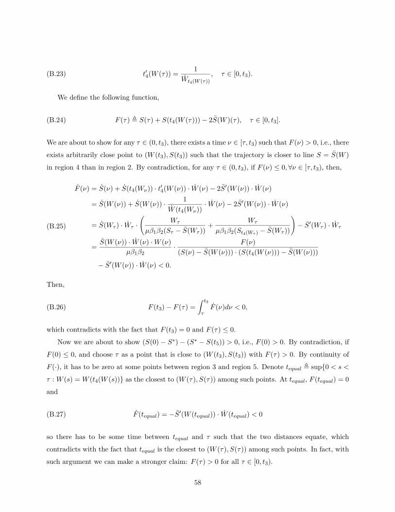
(B.23) t′4(W (τ)) = 1Wt4(W (τ))

, τ ∈ [0, t3).

We define the following function,

(B.24) F (τ) , S(τ) + S(t4(W (τ)))− 2S(W )(τ), τ ∈ [0, t3].

We are about to show for any τ ∈ (0, t3), there exists a time ν ∈ [τ, t3) such that F (ν) > 0, i.e., there

exists arbitrarily close point to (W (t3), S(t3)) such that the trajectory is closer to line S = S(W )

in region 4 than in region 2. By contradiction, for any τ ∈ (0, t3), if F (ν) ≤ 0, ∀ν ∈ [τ, t3), then,

(B.25)

F (ν) = S(ν) + S(t4(Wν)) · t′4(W (ν)) · W (ν)− 2S′(W (ν)) · W (ν)

= S(W (ν)) + S(W (ν)) · 1W (t4(Wν))

· W (ν)− 2S′(W (ν)) · W (ν)

= S(Wτ ) · Wτ ·(

Wτ

µβ1β2(Sτ − S(Wτ ))+ Wτ

µβ1β2(St4(Wτ ) − S(Wτ ))

)− S′(Wτ ) · Wτ

= S(W (ν)) · W (ν) ·W (ν)µβ1β2

· F (ν)(S(ν)− S(W (ν))) · (S(t4(W (ν)))− S(W (ν)))

− S′(W (ν)) · W (ν) < 0.

Then,

(B.26) F (t3)− F (τ) =∫ t3

τF (ν)dν < 0,

which contradicts with the fact that F (t3) = 0 and F (τ) ≤ 0.

Now we are about to show (S(0)− S∗)− (S∗ − S(t5)) > 0, i.e., F (0) > 0. By contradiction, if

F (0) ≤ 0, and choose τ as a point that is close to (W (t3), S(t3)) with F (τ) > 0. By continuity of

F (·), it has to be zero at some points between region 3 and region 5. Denote tequal , sup{0 < s <

τ : W (s) = W (t4(W (s))} as the closest to (W (τ), S(τ)) among such points. At tequal, F (tequal) = 0

and

(B.27) F (tequal) = −S′(W (tequal)) · W (tequal) < 0

so there has to be some time between tequal and τ such that the two distances equate, which

contradicts with the fact that tequal is the closest to (W (τ), S(τ)) among such points. In fact, with

such argument we can make a stronger claim: F (τ) > 0 for all τ ∈ [0, t3).

58

We still need to show that not only F (0) > 0, but also there exists a ϕr > 0 such that F (0) > ϕr

as long as the trajectory does not enter the local stability region, i.e., either |W (t) −W ∗| > ε or

|S(t)− S(W (t))| > ε for any (W (t), S(t)).

Recall from equation (B.25) that

(B.28)F (τ) = S(τ) · W (τ) ·W (τ)

µβ1β2· F (τ)

(S(τ)− S(W (τ))) · (S(t4(W (τ)))− S(W (τ)))

− S′(W (τ)) · W (τ).

Define

(B.29) G(τ) , S(τ) · W (τ) ·W (τ)µβ1β2(S(τ)− S(W (τ))) · (S(t4(W (τ)))− S(W (τ)))

, τ ∈ [0, t3].

Then,

(B.30) F (τ) = G(τ) · F (τ)− S′(W (τ)) · W (τ).

Note that G(0) = 0, and because of continuity of G(·), for a small εG such that

(B.31) 0 < εG <β2ζ(ε− ε−)W ∗(W ∗ + ε) −

β2∆W ∗

where 0 < ∆ < ζ(ε−ε−)W ∗+ε , there exists tG > 0 such that for t ∈ [0, tG), |G(t)| < εG.

Recall that for W ∈ [W ∗,W ∗ + min{δε, ε}), W > µβ1β2(ε−ε−)W ∗+ε . At the same time, the starting

position in region 1 satisfies S(0) ≤ W ∗/β2. S(τ) ≤ S(0) ≤ W ∗/β2 for all τ ∈ [0, t1], because

the trajectory first decreases until it reaches region 5 and then increases to return to region 1 at a

lower level. Therefore, we also have W < µβ1β2(W ∗/β2+ε−)W ∗ . Then for time τ ∈ [0, (W ∗+min{δ,ε})W ∗

µβ1β2(W ∗/β2+ε−)),

W ∈ [W ∗,W ∗ + min{δ, ε}).

F (τ) < S(τ) ≤ W ∗/β2 is bounded. So is S′(W (τ)) > 1µβ1β2

(µ(β1 + β2)− Λβ>χ(W )

)≥

ζ/µβ1β2.

For τ ∈ [0,min{tG, (W ∗+min{δ,ε})W ∗µβ1β2(W ∗/β2+ε−)}),

(B.32)

F (τ) < εGF (τ)− ζ∗µβ1β2

µβ1β2(ε− ε−)W ∗ + ε

<

(β2ζ(ε− ε−)W ∗(W ∗ + ε) −

β2∆W ∗

)· W

∗

β2− ζ(ε− ε−)

W ∗ + ε

= −∆.

59

Therefore,

(B.33)

F (0) > F (0)− F(

min{tG,

(W ∗ + min{δ, ε})W ∗

µβ1β2ε

})> ∆ ·min

{tG,

(W ∗ + min{δ, ε})W ∗

µβ1β2ε

}.

We can make analogous claims on (S∗ − S(t5)) − (S(t1) − S∗), i.e., on the other half of the

trajectory from region 5 back to region 1, and thus prove that in each cycle the trajectory gets

closer to the equilibrium with a positive step size as long as it does not enter the local stability

region and therefore has to converge. �

C. Auxiliary empirical results

% of Variance Explained % of Variance ExplainedOne Factor Two Factors One Factor Two Factors

Alcoa 62% 77% JPMorgan 68% 82%American Express 68% 80% Kraft 74% 84%

Boeing 52% 66% Coca-Cola 71% 82%Bank of America 73% 84% McDonalds 64% 76%

Caterpillar 31% 51% 3M 31% 51%Cisco 76% 87% Merck 76% 86%

Chevron 38% 59% Microsoft 74% 90%DuPont 59% 74% Pfizer 76% 84%Disney 74% 83% Procter & Gamble 72% 81%

General Electric 80% 91% AT&T 69% 81%Home Depot 85% 92% Travelers 75% 85%

Hewlett-Packard 71% 84% United Tech 39% 55%IBM 27% 53% Verizon 76% 87%Intel 74% 86% Wal-Mart 77% 85%

Johnson & Johnson 71% 82% Exxon Mobil 54% 69%

Table 17: Results of PCA for queue lengths trajectories: how much variance in the data can the firsttwo principle components explain.

60