Optimal Monetary Policy with Labor Market Frictions: The ...
39
* † * †
Transcript of Optimal Monetary Policy with Labor Market Frictions: The ...

Optimal Monetary Policy with Labor Market Frictions:
The Role of the Wage Channel∗
Takeki Sunakawa†
Abstract
This paper introduces right-to-manage bargaining into a labor search model with
sticky prices instead of standard e�cient bargaining and examines the Ramsey-optimal
monetary policy. Without real wage rigidity, even when the steady state is ine�-
cient, price stability is nearly optimal in response to technology or government shocks.
Right-to-manage bargaining creates the wage channel to in�ation, as there is a direct
relationship between real wages and real marginal cost. In the presence of the wage
channel, price markups consist of only real marginal cost, and real wages and hours per
worker are determined such as in the Walrasian labor market.
Keywords: Ramsey-optimal monetary policy; Right-to-manage bargaining; Wage chan-
nel; Real wage rigidity; Wage markups
JEL codes: E52; E24
∗This paper is originally a part of the dissertation by the author at The Ohio State University. Theauthor is especially grateful to Bill Dupor and Paul Evans for valuable guidance and support. The authoralso appreciates the comments and discussions from anonymous referees, Hiroki Arato, Ippei Fujiwara,Naohisa Hirakata, Ryoichi Imai, Masaru Inaba, Aubhik Khan, Kengo Nutahara, Pau Rabanal, PaulinaRestrepo-Echavarria, Murat Tasci, Julia Thomas, Kenneth West (the editor), Alexander Wolman, WillemVan Zandweghe, and Francesco Zanetti, as well as seminar participants at The Ohio State University, theCanon Institute for Global Studies, Kansai University, Econometric Society Meetings 2011, the Bank ofEngland, Shinshu University, and University of Tsukuba. Any remaining errors are the author's.†Assistant Professor at Graduate School of Public Policy, the University of Tokyo. E-mail address:
1

1 Introduction
In the study of the Ramsey-optimal monetary policy in models with sticky prices and search
frictions in the labor market, it is usually assumed that real wages and hours per worker are
determined by e�cient bargaining (EB) between �rms and workers.1 Under EB, when the
steady state is e�cient (i.e., the Hosios (1990) condition is met and there is a subsidy to
o�set the distortion stemming from monopolistic competition), price stability to technology
shocks is exactly optimal (Thomas, 2008). The further we deviate from the e�cient steady
state, the more deviation from price stability becomes optimal, as endogenous price markups
stemming from the net hiring cost lead to a tradeo� between in�ation and unemployment
(Faia, 2009).
However, in actual practice, �rms have the right to manage workers; typically, hours
per worker are unilaterally picked by �rms rather than determined by bargaining between
�rms and workers. Then, real wages are determined by bargaining given the labor demand
schedule of �rms. Nickell and Andrews (1983) and Trigari (2006) introduced right-to-manage
(RTM) bargaining into labor search models instead of EB, based on empirical backgrounds.2
This paper studies the Ramsey-optimal monetary policy in a labor search model with
sticky prices and compares the two bargaining schemes, EB and RTM. The results under
RTM contrast starkly with the ones under EB. Even when the steady state is ine�cient,
price stability is nearly optimal under RTM, as opposed to Faia (2009). This is in line with
previous studies of optimal monetary policy in models with sticky prices and the Walrasian
labor market.3 Also, when the steady state is e�cient, the price stability result does not
exactly hold under RTM, as opposed to Thomas (2008).
Under RTM, there is a direct transmission from real wages to real marginal cost, hence
leading to in�ation. This is called the wage channel to in�ation (Christo�el and Kuester,
2008). In the presence of the wage channel, price markups consist of only real marginal cost,
and real wages and hours per worker are determined such as in the Walrasian labor market
with variable wage markups.
Some papers have argued that real wage rigidity is important in explaining empirical
regularities in labor search models.4 With real wage rigidity, deviation from price stability
becomes optimal under both EB and RTM, although the reasons are quite di�erent. When
real wages are sluggish and cannot respond immediately to a positive technology shock,
�rms want to increase labor input. Under RTM, as �rms can adjust labor input at the
intensive margin (hours per worker) and hours per worker are more volatile than real wages,
wage markups become countercyclical and volatile; therefore, deviation from price stability is
optimal. Under EB, �rms mainly adjust labor input at the extensive margin (employment),
which generates �uctuations in the net hiring cost and price markups.
2

Recently, a few papers have studied the Ramsey-optimal monetary policy in labor search
models with sticky prices under EB. Faia (2009) used a similar setting to the one presented
in this paper in terms of the timing of events and quadratic price adjustment, but with only
the extensive margin. She found that deviation from price stability was optimal with the
ine�cient steady state. In contrast, Thomas (2008) introduced both of the intensive and
extensive margins and showed that price stability is optimal with the e�cient steady state.
When nominal wage bargaining is staggered, the case against price stability arises. Blan-
chard and Galí (2010) presented a simpler framework and demonstrated the price stability
result. Real wage rigidity à la Hall (2005) creates the case against price stability. Ravenna
and Walsh (2011) derived the objective function of monetary policy by using second-order
approximation of the household's utility and gap terms of unemployment, as well as in�a-
tion and consumption. They explicitly showed how gap terms are related to welfare costs of
search and matching frictions.
This paper examines both cases with an ine�cient and an e�cient steady state, and
compares di�erent methodologies to compute the Ramsey-optimal monetary policies: the
Lagrange and linear-quadratic (LQ) methods. The Lagrange method can be applied even
when the steady state is ine�cient, whereas the LQ method, with �rst-order approximation
of the equilibrium conditions and second-order approximation of the household's utility, is
usually used only when the steady state is e�cient.5 Faia (2009) used the Lagrange method,
whereas Thomas (2008); Blanchard and Galí (2010); Ravenna and Walsh (2011) used the
LQ method. This paper is consistent with the previous studies; under EB, when the steady
state is e�cient, price stability is exactly optimal, and the Lagrange and LQ methods yield
exactly the same result up to �rst order. The further we deviate from the e�cient steady
state, the more volatile optimal in�ation is, and the larger the numerical error between the
Lagrange and LQ methods. Under RTM, however, the optimal volatility of in�ation is not
zero nor minimized even when the steady state is e�cient.
In the next section, the labor search model and the two types of bargaining, EB and RTM,
are introduced. The relationship between the labor market allocation and the wage channel
is also examined. The Ramsey-optimal monetary policies are computed by the Lagrange
and LQ methods, and calibration is discussed in Section 3. Section 4 shows the results. The
case of the ine�cient steady state is �rst considered in Section 4.1, whereas the case of the
e�cient steady state is examined in Section 4.2. Section 5 o�ers a conclusion. Calculations
of the steady state and proofs of propositions are shown in the appendix.
3

2 Model
In this section, the labor search model used for monetary policy analysis is presented.
Quadratic price adjustment costs, as in Rotemberg (1982), two di�erent types of bargaining
(EB and RTM), as in Trigari (2006), and a simple form of real wage rigidity, as in Hall
(2005), are introduced. The relationship between labor market allocation and the di�erent
types of wage bargaining is also discussed.
2.1 Timing of Events
Time is discrete and in�nite: t = 0, 1, 2, ...,∞. The timing of events is as follows:
1. 1−nt−1 is the measure of unemployed workers at the end of the last period. A fraction
of the employed workers ρnt−1 are exogenously separated as
ut = 1− nt−1 + ρnt−1, (1)
where ut workers seek jobs in the current period.
2. Firms post vacancies vt to match with the unemployed workers ut by a matching
functionm(ut, vt), which exhibits constant returns to scale. The labor market tightness
is given by
θt = vt/ut. (2)
Each worker and �rm are small, in the sense that they take as given the labor mar-
ket tightness at the aggregate level θt. The job �nding rate for workers, p(θt) =
m(ut, vt)/ut = m(1, θt), and the job �lling rate for �rms, q(θt) = m(ut, vt)/vt =
m(θ−1t , 1), are also given for them.
3. The number of the newly employed workers is given by
nt = (1− ρ)nt−1 +m(ut, vt). (3)
Note that the newly employed workers can work immediately.6
4. The employed workers enter into production:
yt = atf(ht)nt, (4)
where at is the technology shock. Each employed worker works ht hours and produces
atf(ht), which is the decreasing returns to scale in terms of hours per worker, so that
4

�rms earn a positive pro�t period by period. Total production is linear in nt.
2.2 Households
A family of households chooses consumption ct, one-period nominal bonds Bt that pay gross
interest rate Rt, and the number of the employed workers nt so as to maximize the life-time
utility:
Vt =c1−σt
1− σ− g(ht)nt + βEtVt+1,
subject to
ct +Bt
Pt≤ wthtnt + b(1− nt) +
Rt−1Bt−1
Pt+TtPt,
nt = (1− ρ)nt−1 + (1− nt−1 + ρnt−1)p(θt).
A fraction of households nt are employed and earn wage bill wtht, and 1−nt are unemployed
at the end of the period and receive unemployment bene�ts b. wt is real wage, and ht is
hours per worker, which are determined by bargaining between workers and �rms. Tt is the
sum of transfers from �rms and the government. Pt is the aggregate price index. β ∈ (0, 1) is
a discount factor. σ > 0 is a parameter for the degree of risk aversion. g(ht) is an increasing
function that measures labor disutility. The job �nding rate p(θt) is taken as given by each
worker. Consumption is pooled among households to insure against the unemployment risk;
therefore, households consume the same amount regardless of their employment status (Merz,
1995; Andolfatto, 1996).
By the �rst order necessary conditions (FONCs) of ct and Bt, the standard consumption
Euler equation is derived as
1 = βRtEt
{(ct+1
ct
)−σPtPt+1
}. (5)
The FONC of nt and the envelope theorem yields
St = wtht − g(ht)cσt − b+ β(1− ρ)Et
{(ct+1
ct
)−σ(1− p(θt+1))St+1
}, (6)
where St is the ratio of Lagrange multipliers of the budget constraint and the law of motion
for nt. St is also the matching value of a marginal worker for the family of households.
5

2.3 Firms
There are two types of �rms: a �nal-good producing �rm and di�erentiated intermediate-
good producing �rms. The �nal-good producing �rm purchases each intermediate good yit
at price Pit for i ∈ [0, 1] and minimizes its expenditure Ptyt =∫ 1
0Pityitdi subject to the
Dixit-Stiglitz (1977) aggregator yt =(∫ 1
0y
(εp−1)/εpit di
)εp/(εp−1)
. It yields the demand curve
with the elasticity parameter εp > 1, yit = (Pit/Pt)−εpyt.
Each intermediate-good producing �rm i produces yit in monopolistic competition and
sells it to the �nal-good producing �rm. The intermediate-good producing �rm i chooses
prices and allocations Pit, nit, and vit so as to maximize the discounted sum of future pro�ts
E0
∞∑t=0
βt(ctc0
)−σ{(1 + τ)Pit
Ptyit − withitnit − cvvit −
ψ
2
(PitPit−1
− 1
)2},
subject to
yit = (Pit/Pt)−εpyt = atf(hit)nit,
nit = (1− ρ)nit−1 + vitq(θt),
where βt(ct/c0)−σ is a stochastic discount factor for the �rm. The �rm i sets the intermediate-
good price Pit subject to the downward-sloping demand curve and quadratic price adjustment
costs with the parameter ψ > 0. τ ≥ 0 is a subsidy to �rms to o�set the distortion stemming
from monopolistic competion.7 The �rm i also chooses the amount of employment and
vacancies nit and vit and pays the total wage bill withitnit and vacancy costs cvvit with the
parameter cv > 0. The job �lling rate q(θt) is taken as given by each �rm. The FONCs are
∂Pit : ψ
(PtPt−1
− 1
)PtPt−1
= βEt
{(ct+1
ct
)−σψ
(Pt+1
Pt− 1
)Pt+1
Pt
}
+yt(1− εp)(
(1 + τ)− εpεp − 1
ϕt
), (7)
∂nit : Jt = ϕtatf(ht)− wtht + β(1− ρ)Et
{(ct+1
ct
)−σJt+1
},
∂vit : Jt =cvq(θt)
. (8)
In equilibrium, all of the �rms choose the same prices and allocations, so index i is dropped
in the resulting conditions. The FONC of Pit is a nonlinear version of the Phillips curve. ϕt
is the Lagrange multiplier on the production function and measures real marginal cost. ϕt
is also the price of intermediate goods relative to �nal goods.8
In the FONC of nit, Jt is the Lagrange multiplier on the law of motion for employment
6

and measures the matching value of a marginal job for each �rm. The �rm's pro�t period by
period is given by ϕtatf(ht)− wtht > 0, and the �rm continues to match in the next period
with the probability (1− ρ). Note that the value of a vacancy is zero under the assumption
of free entry, and Jt is equal to the expected cost of vacancy in the FONC of vt. The last
two equations are summarized into the hiring condition:
cvq(θt)
= ϕtatf(ht)− wtht + β(1− ρ)Et
{(ct+1
ct
)−σcv
q(θt+1)
}. (9)
The expected cost of vacancy is equal to the discounted sum of future pro�ts per worker.
The net hiring cost
xt ≡cvq(θt)
− β(1− ρ)Et
{(ct+1
ct
)−σcv
q(θt+1)
}(10)
is also de�ned; employment is a stock, and the net hiring cost includes the bene�t of stock
hoarding in the next period.
2.4 Wage Contracts
As shown in Sections 2.2 and 2.3, matching values of workers and �rms are given by (6)
and (8). A wage bill set [ωt, ωt], which is compatible with their incentive to continue the
matching, is derived from the conditions St ≥ 0 and Jt ≥ 0. ωt is the workers' reservation
wage bill, and ωt is the �rms' reservation wage bill. As long as the wage bill wtht is in the set
[ωt, ωt], workers and �rms continue their matching. To pin down the equilibrium real wages
wt and hours per worker ht within the set, two di�erent types of wage contracts between
workers and �rms are introduced.
2.4.1 E�cient Bargaining
Under EB, real wages and hours per worker (wt, ht) are determined by Nash bargaining
between worker and �rm to maximize the joint surplus Sηt J1−ηt subject to the equations (6)
and (8), where η ∈ (0, 1) is a parameter for workers' actual bargaining power. The FONCs
are
∂ht : ϕtatf′(ht) = g′(ht)c
σt , (11)
∂wt : ηJt = (1− η)St. (12)
7

Equation (11) shows that the marginal rate of substitution is equal to the real marginal
cost times the marginal product of labor. Equation (12) shows that worker's surplus from
bargaining is simply a fraction η of the total surplus, St = η(St+Jt). Plugging the matching
values for workers and �rms, St and Jt given by (6) and (8) into (12), we have
wtht = ηϕtatf(ht) + (1− η) (g(ht)cσt + b)
+ ηβ(1− ρ)Et
{(ct+1
ct
)−σcvθt+1
}. (13)
The wage bill is equal to a weighted average of the workers' reservation wage and the �rms'
reservation wage, wtht = ηωt + (1− η)ωt with a constant weight η.
2.4.2 Right-to-Manage Bargaining
Under RTM, there are two stages in the bargaining in each period. First, real wages wt
are determined by Nash bargaining between workers and �rms so as to maximize the joint
surplus Sηt J1−ηt . Second, �rms choose the level of hours per worker ht so as to solely maximize
the matching value for �rms Jt. In the second stage, given wt, the FONC of ht is
wt = ϕtatf′(ht). (14)
Real wages are equal to the real marginal cost times the marginal product of labor. Equation
(14) implies that �rms have labor demand schedule on real wages, ht = f ′−1(wt/(ϕtat)) ≡h(wt). In the �rst stage, taking the wage schedule into account, workers and �rms bargain
over real wages wt so as to maximize the joint surplus. The FONC of wt is
δt = [(1− η)/η]St/Jt, (15)
where δt ≡ −(∂St/∂wt)/(∂Jt/∂wt) is the marginal gain for workers (relative to marginal loss
for �rms) by incremental real wages. By plugging the matching values for workers and �rms
St and Jt into (15), we have
wtht = χtϕtatf(ht) + (1− χt) (g(ht)cσt + b)
+ χtβ(1− ρ)Et
{(ct+1
ct
)−σ(1− (δt+1/δt)[1− s(θt+1)])
cvq(θt+1)
}, (16)
where χt = ηδt/(1 − η(1 − δt)) is workers' e�ective bargaining power. The wage bill is
equal to a weighted average of the workers' reservation wage and the �rms' reservation wage,
wtht = χtωt + (1− χt)ωt with a time-varying weight χt.
8

2.4.3 Real Wage Rigidity
Under both EB and RTM, workers and �rms bargain over real wages period by period. Real
wage rigidity is introduced into the model in the form of Hall's (2005) real wage norm
wt = (1− γw)w∗t + γwwt−1, (17)
where wt is the actual wage and w∗t is the target wage determined by bargaining. γw is
a parameter for the degree of real wage rigidity. Although the wage norm itself is an ad-
hoc assumption and not considered when the target wage is determined, the framework
encompasses various sources of wage rigidity at a more primitive level, such as in Hall and
Milgrom (2008) and Gertler and Trigari (2009). This type of wage rigidity is also robust to
the Barro's (1977) critique; as long as the actual wage bill is inside the wage bill set [ωt, ωt],
both the workers and �rms have an incentive to continue the matching.
2.5 Closing the Model
The resource constraint, including posting vacancies and price adjustment costs and unem-
ployment bene�t, is given by
ct + gt + cvvt +ψ
2π2t = yt + (1− nt)b, (18)
where gt is the government expenditure. Note that all �rms set the same price so that∫ 1
0ψ2
(Pit
Pit−1− 1)2
di = (ψ/2)π2t , where πt = Pt/Pt−1 − 1 is the in�ation rate. To close the
model, the Ramsey-optimal policy is given in Section 3.
Competitive equilibrium is de�ned by the equilibrium conditions (1)-(9), (11), and (13)
under EB or (14) and (16) under RTM, (17) and (18) under the Ramsey-optimal policy such
that (i) households maximize their utility, (ii) �rms maximize their pro�ts, (iii) wages and
hours per worker are determined via bargaining between �rms and workers, and (iv) the
markets clear.
2.6 Labor Market Allocation and the Wage Channel
Labor market allocation is characterized by equations (11) and (13) under EB or (14) and
(16) under RTM. In (14), real wages have a direct link to real marginal cost and hence
in�ation. As �rms choose the level of hours per worker, real wages are equal to the real
marginal cost times the marginal product of labor. Christo�el and Kuester (2008) called
this transmission mechanism the wage channel to in�ation. Real wage rigidity is irrelevant
9
to in�ation persistence under EB (Krause and Lubik, 2007), whereas it is relevant under
RTM (Christo�el and Linzert, 2010).
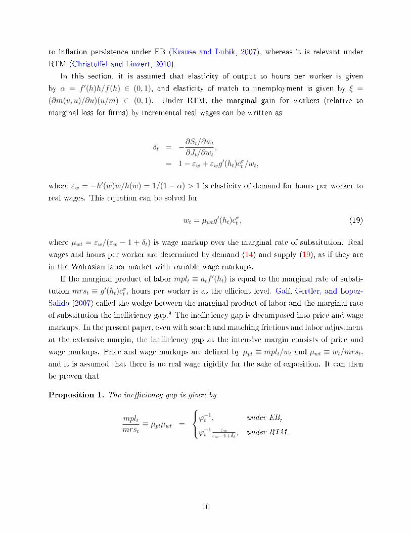
In this section, it is assumed that elasticity of output to hours per worker is given
by α = f ′(h)h/f(h) ∈ (0, 1), and elasticity of match to unemployment is given by ξ =
(∂m(v, u)/∂u)(u/m) ∈ (0, 1). Under RTM, the marginal gain for workers (relative to
marginal loss for �rms) by incremental real wages can be written as
δt = −∂St/∂wt∂Jt/∂wt
,
= 1− εw + εwg′(ht)c
σt /wt,
where εw = −h′(w)w/h(w) = 1/(1− α) > 1 is elasticity of demand for hours per worker to
real wages. This equation can be solved for
wt = µwtg′(ht)c
σt , (19)
where µwt = εw/(εw − 1 + δt) is wage markup over the marginal rate of substitution. Real
wages and hours per worker are determined by demand (14) and supply (19), as if they are
in the Walrasian labor market with variable wage markups.
If the marginal product of labor mplt ≡ atf′(ht) is equal to the marginal rate of substi-
tution mrst ≡ g′(ht)cσt , hours per worker is at the e�cient level. Galí, Gertler, and Lopez-
Salido (2007) called the wedge between the marginal product of labor and the marginal rate
of substitution the ine�ciency gap.9 The ine�ciency gap is decomposed into price and wage
markups. In the present paper, even with search and matching frictions and labor adjustment
at the extensive margin, the ine�ciency gap at the intensive margin consists of price and
wage markups. Price and wage markups are de�ned by µpt ≡ mplt/wt and µwt ≡ wt/mrst,
and it is assumed that there is no real wage rigidity for the sake of exposition. It can then
be proven that
Proposition 1. The ine�ciency gap is given by
mpltmrst
≡ µptµwt =
ϕ−1t , under EB,
ϕ−1t
εwεw−1+δt
, under RTM,
10

where price and wage markups are
µpt =
ϕ−1t α
(1 + xt
wtht
), under EB,
ϕ−1t , under RTM,
(20)
µwt =
α−1(
1 + xtwtht
)−1
, under EB,
εwεw−1+δt
, under RTM.(21)
Proof. See Appendix A.2.1.
Under EB, �rms adjust labor input only at the extensive margin, as hours per worker
is determined by bargaining, and µEBpt = ϕ−1t α
(1 + xt
wtht
)holds. This includes endogenous
price markups related to the net hiring cost of labor adjustment at the extensive margin
(Faia, 2009). Under RTM, �rms adjust labor input not only at the extensive margin but also
at the intensive margin; �rms choose the level of hours per worker and smooth out the net
hiring cost; α(
1 + xtwtht
)= 1 holds under RTM. This implies µRTMpt = ϕ−1
t ; price markups
consist of only real marginal cost.
Under EB, wage markups just o�set price markups related to the net hiring cost, µEBwt =
α−1(
1 + xtwtht
)−1
so that the ine�ciency gap consists of only real marginal cost measuring
ine�ciency in the goods market. Under RTM, the ine�ciency gap also includes endogenous
wage markups µRTMwt = εw/(εw − 1 + δt) regarding ine�ciency in the labor market.
Under RTM, the allocation in the decentralized economy is not e�cient, even when the
standard Hosios condition is satis�ed (Sunakawa, 2012). It can be proven that
Proposition 2. The allocation in the decentralized economy is e�cient in the steady state
if and only if ϕ = 1 and
η = ξ, under EB,
η = ξ = χ, under RTM.
Also, the allocation in the e�cient steady state is common between EB and RTM.
Proof. See Appendix A.2.2.
The e�ciency condition under RTM imposes more parameter restriction than the stan-
dard Hosios condition under EB, as the e�ective workers' bargaining power, χ = ηδ/(1 −η(1 − δ)), depends on δ and hence other variables. Therefore, from the viewpoint of its
empirical relevance, the case of the ine�cient steady state is �rst considered in Section 4.1,
whereas the case of the e�cient steady state is also examined in Section 4.2.
11

3 Optimal policy and calibration
The equilibrium conditions in the previous section are summarized into (c.f., Schmitt-Grohé
and Uribe (2004)):
Et {fi(yt+1,yt,xt+1,xt)} = 0,
where fi is the (possibly nonlinear) equilibrium conditions for i = 1, ..., n− 1, xt is a nx × 1
vector of the state variable, yt is a ny×1 vector of the jump variable, and n = nx+ny. There
are n− 1 equilibrium conditions and n variables. The Ramsey-optimal policy pins down the
equilibrium (if it exists and is unique) yt = g∗(xt;σε) and xt+1 = h∗(xt;σε) + ηεσεεt+1.
3.1 Ramsey-Optimal Policies
The Ramsey-optimal policy yields the constrained e�cient equilibrium, which can be ob-
tained by maximizing the representative household's utility subject to the equilibrium condi-
tions of the economy. There are two di�erent methodologies to compute the Ramsey-optimal
policies: the Lagrange and LQ methods.
In the Lagrange method, the Ramsey-optimal policy is computed by using the Lagrangean
L0 = min{Λt}∞t=0
max{Ξt}∞t=0
E0
{∞∑t=0
βtEt
{U(xt,yt) +
n−1∑i=1
λitfi(yt+1,yt,xt+1,xt)
}},
where Λt is the set of Lagrange multipliers, Ξt is the set of endogenous variables, and U
is the household's utility period by period. The Lagrangean yields n �rst-order necessary
conditions and n− 1 Lagrange multipliers; therefore, there are 2n− 1 equilibrium conditions
and unknowns.
In the LQ method, the household's utility U is approximated up to second order, and
the equilibrium conditions fis are approximated up to �rst order in the Lagrangean shown
above. Benigno and Woodford (2012, Proposition 1) showed that, if the household's utility
is correctly approximated, the Lagrange and LQ methods are exactly the same up to �rst
order. However, computing the correct LQ approximation can be very tedious. All the
linear terms in the approximated household's utility are substituted out by using second-
order approximation of the equilibrium conditions so that the household's utility is purely
quadratic. When the steady state is e�cient, such a computation is relatively easier as
follows:
Proposition 3. When the steady state is e�cient, under both EB and RTM, the discounted
12

sum of the household's utility is approximated as
V0 − V ≈ −c1−σ
2E0
∞∑t=0
βt{ψ
cπ2t + σc2
t −y
c(y2t − n2
t )
− αy/c1 + φ
(n2t −
[nt + (1 + φ)ht
]2)
+cvv/c
1− ξ(ξu2
t + (1− ξ)v2t − m2
t
)},
where xt = ln(xt/x) is the log deviation from the steady state.
Proof. See Appendix A.2.3.
Note that the e�cient steady state is common between EB and RTM, and so is the correct
LQ approximation. The correct LQ approximation is used to compute the Ramsey-optimal
policies in the case of the e�cient steady state in Section 4.2.
3.2 Calibration
Functional forms are assumed as follows. The production function is f(ht) = hαt , where
α ∈ (0, 1) is elasticity of production to hours per worker. The labor disutility is g(ht) =
κh1+φt /(1 + φ), where φ > 0 is the inverse of Frisch elasticity and κ > 0 is a normalization
parameter. The matching function is m(ut, vt) = muξtv1−ξt , where ξ ∈ (0, 1) is elasticity of
matches to unemployment and m > 0 is a normalization parameter. Unemployment bene�ts
are given by b = bwwh, where bw ∈ (0, 1) is the ratio of unemployment bene�t to the wage
bill.
Parameter values are calibrated following previous studies based on the postwar U.S. data
and summarized in Table 1.10 Steady state unemployment after matching 1 − n = 0.4 and
�lling vacancy rates for �rms q = 0.7 are given as the calibration targets.11 β = 0.99 implies
that the annual interest rate is 4%. The risk aversion parameter is set to σ = 2. εp = 6
implies that the steady state price markup is 20%. The ratio of government expenditure to
output is 25%. These values are standard and in line with the postwar U.S. data. The price
adjustment cost parameter ψ = 20 implies that the elasticity of in�ation to real marginal
cost in the log-linearized Phillips curve is (εp − 1)y/ψ = 0.15. The job destruction rate
ρ = 0.1 and elasticity of matches to unemployment ξ = 0.4 are also standard. The ratio of
unemployment bene�t to wage bill is bw = 0.6. Elasticity of production to hours per worker
is α = 0.9, which also implies elasticity of labor demand to real wages at the intensive margin
εw = 1/(1 − α) = 10. The inverse of Frisch elasticity is φ = 2. The shock parameters are
13

assumed ρa = 0.95 and σa = 0.008, following the evidence on the Solow residual from the
postwar U.S. data.
[Table 1 is inserted here]
In the case of the ine�cient steady state in Section 4.1, η > ξ = 0.4, and the Hosios
condition is not met under EB. Given the values of η and ξ, the marginal gain for workers
by incremental real wages is δ = 0.26 < 1 and the wage markup is µw = w/mrs = 1.08 > 1
in the steady state under RTM, as shown in Table 2, which implies that there is a positive
ine�ciency gap in the labor market (Galí, Gertler, and Lopez-Salido, 2007). The ine�ciency
gap also implies that the workers' e�ective bargaining power χ = δη/(1− η + δη) = 0.28 is
less than the workers' actual bargaining power η = 0.6. When η = ξ = 0.225, η = ξ = χ
holds and the steady state is e�cient under both EB and RTM, as shown in Proposition 2,
which is the case examined in Section 4.2.
[Table 2 is inserted here]
4 Results
In this section, the Ramsey-optimal monetary policies are numericaly investigated. First,
the case of the ine�cient steady state (Faia, 2009) without and with real wage rigidity
is examined in Section 4.1. The case of the e�cient steady state (Thomas, 2008) and a
comparison between the Lagrange and LQ methods are shown in Section 4.2.
4.1 The ine�cient steady state
In the case of the ine�cient steady state, it is shown that price stability in response to
technology shocks is nearly optimal in the model with RTM without real wage rigidity. This
result starkly contrasts with the Faia's (2009) result in the model with EB, and is in line with
the result in a model with the Walrasian labor market. With real wage rigidity, deviation
from price stability becomes optimal. Under RTM, the optimal volatility of in�ation is high
when the workers' bargaining power is low, which also o�ers an interesting contrast with
Faia's result. Similarly, a larger unemployment bene�t to amplify the labor market volatility
(Hagedorn and Manovskii, 2008) does not increase the optimal volatility of in�ation under
RTM, whereas it does under EB.
14

4.1.1 Without real wage rigidity
Figure 1 shows the impulse responses to a technology shock (0.8 = 100σa%) without real
wage rigidity under both EB and RTM. First of all, price stability is nearly optimal under
RTM; namely, the optimal response of in�ation to a positive technology shock is very small.
In response to a positive technology shock, under RTM, real wages respond immediately,
and �rms post more vacancies to produce more. A larger labor demand makes the aggregate
labor market condition tighter, and employment gradually adjusts so that the labor supply
is increased. Under EB, real wages are sluggish even without real wage rigidity, which makes
the labor market condition even tighter. In�ation deviates from zero and responds negatively.
[Figure 1 is inserted here]
What is the intuition behind the di�erent results under EB and RTM? Under EB, as in
Faia (2009), endogenous price markups stemming from the net hiring cost and a related trade-
o� between in�ation and unemployment undo price stability, even with both the intensive
and extensive margins, compared to the case with the extensive margin only in Faia (2009).
Under RTM, real wages and hours per worker replicate the allocation in the Walrasian labor
market with variable wage markups. The wage channel to in�ation leads to stable price
markups, as they consists of only real marginal cost.
The left column of Figure 2 breaks down the ine�ciency gap into the price and wage
markups, as shown in Proposition 1. Under EB, the price markup responds positively,
as the net hiring cost is higher with a tighter labor market condition. The wage markup
responds negatively to o�set the labor market ine�ciency measured by the ine�ciency gap.
The gap responds positively, as the former e�ect dominates the latter. Under RTM, the wage
markup responds negatively, but it stems from δt in Equation (19), as the marginal gain for
workers (relative to the marginal loss for �rms) by incremental real wages gets larger. Price
markups are stable in response to the shock, and wage markups are the main driving force
of the ine�ciency gap.
The allocation in a model with the Walrasian labor market is also computed in Figure
3. Real wages and hours per worker are determined by wt = mrst = ϕtmplt. The divine
coincidence in Blanchard and Galí (2007) holds and �uctuations in the price and wage
markups are exactly zero. The price stability result under RTM is a quantitative one, as
opposed to the case with the Walrasian labor market.12
[Figure 2 is inserted here]
15

4.1.2 With real wage rigidity
Figure 3 shows the impulse responses with real wage rigidity. It is shown that deviation
from price stability is optimal both under EB and RTM. Real wages are sluggish and cannot
respond immediately to a positive technology shock. Firms post even more vacancies, and
the aggregate labor market condition becomes even tighter to take advantage of lower real
wages, especially under EB, because �rms mainly adjust labor input at the extensive margin,
as hours per worker is determined by bargaining.13
Under RTM, sluggish real wages make wage markups countercyclical and volatile because
the marginal rate of substitution is related to real wages, as shown in the labor supply
equation (19). Hours per worker increase, as �rms can adjust labor input at the intensive
margin. Under EB, �rms adjust labor input mainly at the extensive margin and hours per
worker decreases instead because there is no direct link between real wages and hours per
worker. Price markups respond strongly, re�ecting aggressive adjustments at the extensive
margin, whereas wage markups are relatively stable compared to the ones under RTM.
[Figure 3 is inserted here]
The right column of Figure 2 also breaks down the ine�ciency gap into price and wage
markups in the case with real wage rigitity. As in the case without real wage rigidity,
price markups are volatile and wage markups just o�set the gap under EB, whereas wage
markups mainly explain �uctuations in the gap under RTM. The responses under RTM
closely resemble the ones in the model with the Warlasian labor market.
Under RTM, the allocational role of real wages is the key to explain the equilibrium
dynamics. Firms can adjust labor input at the intensive margin and take advantage of low
and sluggish real wages by increasing hours per worker via the wage channel. The adjustment
at the intensive margin, however, yields wage markup �uctuations and makes the optimal
in�ation volatile, depending on the degree of real wage rigidity, as in the model with the
Walrasian labor market. Under EB, the allocational role of real wages is limited, as there is
no direct link between real wages and hours per worker. Firms mainly adjust labor input at
the extensive margin, which generates �uctuations in the net hiring cost and price markups.
4.1.3 Robustness checks
The price stability result under RTM without real wage rigidity is a quantitative one. Some
robustness checks are done for di�erent shocks and parameter values. The analysis herein
focuses on the case without real wage rigidity.
16

Government expenditure shocks Figure 4 shows the response to a positive government
expenditure shock in the case without real wage rigidity. Faia (2009) showed that in response
to the government expenditure shock, deviation from price stability arises, although the re-
sponse is rather small. Faia's result depends on the assumption that �rms adjust labor input
at the extensive margin only. When φ = 104 so that adjusting at the intensive margin is too
costly, the model under EB in this paper replicates the case with the extensive margin only
in Faia (2009). Employment decreases through a lower tightness of labor market. However,
when φ = 2 so that �rms also adjust labor input at the intensive margin, employment in-
creases as well as the labor market tightness and hours per worker, which leads to more price
markup �uctuation and deviation from price stability. Under RTM, employment decreases
insteadly, whereas hours per worker increase. The response of price markups is muted, and
price stability is as nearly optimal as in the case of technology shocks.
[Figure 4 is inserted here]
Di�erent values of η and bw Faia (2009) showed that the optimal volatility of in�ation
is increasing in η because a higher bargaining power η results in more external congestion
and unemployment �uctuations under EB. The left window of Figure 5 shows the optimal
volatility of in�ation for di�erent values of η under both EB and RTM.14 Under EB, it
replicates Faia's result.15 Under RTM, the optimal volatility of in�ation is high when η is
low. The external congestion is irrelevant to the optimal in�ation because �rms can smooth
the net hiring cost at the extensive margin by adjusting labor input at the intensive margin.
When η is low (i.e., when �rms have more bargaining power), �rms adjust hours per worker
in the presence of the wage channel, and wage markups become more volatile.16
Hagedorn and Manovskii (2008, hereafter HM) showed that a larger value of unemploy-
ment bene�t, b = bwwh, also yields a larger employment �uctuation under EB.17 The right
window of Figure 5 shows the optimal volatility of in�ation for di�erent values of bw. Under
EB, the larger bw, the more volatile in�ation is. The labor market condition becomes more
volatile, as pointed out by HM. Under RTM, however, the wage channel kills the labor mar-
ket volatility. The optimal volatility of in�ation is high when bw is low because workers want
to work more with a lower outside option, which makes hours per worker and wage markups
volatile.
[Figure 5 is inserted here]
17

4.2 The e�cient steady state
The case of the e�cient steady state is examined to compare it with the price stability result
under EB in Thomas (2008). If and only if ϕ = 1 and ξ = η = χ, the steady state is e�cient
and common between EB and RTM, as shown in Proposition 2. The condition for e�ciency
in the steady state is satis�ed when ξ = η∗ = 0.225, with the calibration in Section 3.2. The
correct LQ approximation is also common between EB and RTM, as shown in Proposition
3, and is used to compute the Ramsey-optimal monetary policies.
Figure 6 shows the impulse responses to a technology shock (0.8 = 100σa%) without
real wage rigidity under both EB and RTM. When the steady state is e�cient, the optimal
response of in�ation is exactly zero as in Thomas (2008). The reason is understood by ex-
amining Figure 7, which shows the decomposition of the ine�ciency gap. Without real wage
rigidity, under EB, the price and wage markups cancel each other out, and the ine�ciency
gap is exactly equal to zero. In other words, there is no external congestion. Thus, the mon-
etary policymaker can focus on stabilizing in�ation. Under RTM, even though the (logged)
ine�ciency gap is zero in the e�cient steady state, it temporally deviates from zero due to
wage markup �uctuations. With real wage rigidity, deviation from price stability is optimal
under both EB and RTM. The responses of price and wage markups under RTM resemble
the ones in the model with the Walrasian labor market, as in the case of the ine�cient steady
state.
Figure 8 shows the optimal volatility of in�ation for di�erent values of η. It is shown that
the optimal volatility of in�ation is zero under EB when ξ = η∗, as in Thomas (2008). On
the contrary, under RTM, even when ξ = η∗, the optimal volatility of in�ation is not zero
nor minimized over η. The optimal volatility of in�ation computed by the LQ method are
shown with gray lines in Figure 8. When ξ = η∗, the optimal volatilities computed by the
Lagrange and LQ methods are exactly the same under both EB and RTM.
The results of the paper are consistent with the ones in Thomas (2008) [price stability
when the steady state is e�cient] and Faia (2009) [deviation from price stability when the
steady state is ine�cient]. It is found that, when the steady state is e�cient, the price
stability result holds under EB, and the LQ and Lagrangean methods yield exactly the same
results up to �rst order. When the steady state is ine�cient, deviation from price stability
arises, and the further we deviate from the e�cient steady state, the larger the numerical
error between the Lagrange and LQ methods.
[Figure 6-8 is inserted here]
18

5 Concluding Remarks
This paper analyzed the Ramsey-optimal monetary policy in labor search models with sticky
prices, focusing on the role of the wage channel to in�ation (i.e., a relationship between real
wages and real marginal cost), based on empirical evidence. It is found that the nature
of the Ramsey-optimal monetary policy under RTM is totally di�erent from the one under
EB. Under RTM, even when the steady state is ine�cient, price stability is nearly optimal,
whereas deviation from price stability is optimal under EB. Real wage rigidity creates the
case against price stability, as hours per worker are more volatile than real wages, and wage
markups are countercyclical and volatile, as in models with the Walrasian labor market.
This paper also studied both cases with the ine�cient and the e�cient steady state. Under
EB, price stability is optimal with the e�cient steady state, and the more we deviate from
the e�cient steady state, the more volatilie optimal in�ation is. Under RTM, however, even
when the steady state is e�cient, the optimal volatility of in�ation is not zero nor minimized.
In the present paper, it is found that wage markups are countercyclical and volatile with
the wage channel and real wage rigidity. In the U.S. economy, the ine�ciency gap between
the marginal product of labor and the marginal rate of substitution is mainly explained
by countercyclical wage markup �uctuations, as shown in Galí, Gertler, and Lopez-Salido
(2007); therefore, one of the interesting topics for future research will be to investigate this
relationship more. Within the search and matching framework, the wage channel and real
wage rigidity are potentially able to explain the labor wedge (Chari, Kehoe, and McGrattan,
2007), which is one of the main drivers for business cycles (Cheremukhin and Restrepo-
Echavarria, 2014; Pescatori and Tasci, 2011).
A Appendix
A.1 Steady State
r = 1/β and ϕ = (1 + τ)(εp − 1)/εp are immediately obtained. Given the steady state
unemployment u = 1 − n and job �lling rate q = m/v, the other steady state values of the
labor market are
n = 1− u, v = ρn/q, m = ρn/(uξv1−ξ),
u = 1− n+ ρn, θ = v/u, p = ρn/u,
which are common between the two bargaining schemes.
19

A.1.1 E�cient Bargaining
We normalize a = 1. Steady state conditions of matching values S and J are given by
ϕαhα−1 = κhφcσ,
[1− β(1− ρ)(1− p)]S = (1− bw)wh− κh1+φcσ/(1 + φ),
[1− β(1− ρ)]J = ϕhα − wh,
1 = [(1− η)/η]S/J,
These equations can be solved for
wh =η[1− β(1− ρ)(1− p)] + (1− η)[1− β(1− ρ)]α/(1 + φ)
η[1− β(1− ρ)(1− p)] + (1− η)[1− β(1− ρ)](1− bw)xhα,
S, and J . Given q and J , vacancy cost is cv = qJ and steady state consumption c =
hαn− g− cvv− (1−n)b gets pinned down. With the calibration given in Section 3.2, steady
state vacancy cost is about 2.18% of output and steady state consumption is about 72.82%
of output. Steady state reservation wage bills for workers and �rms are given by ω = wh−Sand ω = wh+ J . Using the calibrated parameters, [ω, ω] = [0.5952, 1.2699]wh is obtained.
A.1.2 Right-to-Manage Bargaining
Steady state conditions of matching values are given by
wh = ϕαhα,
[1− β(1− ρ)(1− p)]S = (1− bw)wh− κh1+φcσ/(1 + φ),
[1− β(1− ρ)]J = ϕhα − wh,
δ = [(1− η)/η]S/J,
These equations can be solved for
δ =(1− η)[(1 + φ)(1− bw)− α][1− β(1− ρ)]α
η[1− β(1− ρ)(1− p)](1 + φ)(1− α) + (1− η)[1− β(1− ρ)]α(1− α), (22)
S, and J . Steady state vacancy cost is about 7.65% of output and steady state consumption
is about 67.35% of output. [ω, ω] = [0.5952, 2.0194]wh is obtained.
20

A.2 Proofs
A.2.1 Proposition 1
For price markups, under both EB and RTM, the hiring condition (9) at the extensive margin
becomes
ϕt =
(1 +
xtwtht
)wthtntyt
,
=
(1 +
xtwtht
)αwtmplt
,
where mplt ≡ atf′(ht) = αyt/(htnt); therefore, µ
EB
pt = ϕ−1t α
(1 + xt
wtht
). Under RTM, in
addition to the hiring condition, the wage channel (15) becomes
wt = ϕtatf′(ht),
= ϕtmplt.
Price markups are equal to the inverse of real marginal cost, i.e., µRTMpt = ϕ−1t , which also
implies α(1 + xt/(wtht)) = 1; the net hiring cost is smoothed.
For wage markups, under EB, the bargaining between �rms and workers over hours per
worker yields the e�ciency condition (11) at the intensive margin;
mrst = ϕtmplt,
which implies that the ine�ciency gap is equal to the inverse of real marginal cost. Wage
markups are given by µEBwt = wt/(ϕtmplt) = 1/(ϕtµEB
pt ) = α−1(
1 + xtwtht
)−1
. Under RTM,
equation (11) does not hold, and the wage equation (16) becomes
wt = µRTMwt mrst,
where µRTMwt = εwεw−1+δt
. The e�ciency gap is given by µRTMpt µRTMwt = ϕ−1t
εwεw−1+δt
.
Figure 9 graphically shows how real wages and hours per worker (w, h) are determined.18
Under EB, by equation (11), hours per worker are determined at h = hEB regardless of
wage contracts. Real wages are determined independently at w = wEB by equation (13).
(wEB, hEB) is determined at the point E1 in Figure 9. If the Hosios (1990) condition is satis�ed
and there is a subsidy to o�set the distortion stemming from monopolistic competition,
real wages and hours per worker are at the e�cient level at the point E0 in Figure 9,
(w∗, h∗). Under RTM, the wage channel yields the labor demand schedule equation (14),
21

whereas the bargaining over real wages between workers and �rms yields the labor supply
schedule equation (19), which shifts with variable wage markups µRTMwt . The equilibrium is
the intersection of the demand and supply at the point E2 in Figure 9, (wRTM, hRTM).
[Figure 9 is inserted here]
A.2.2 Proposition 2
The e�cient equilibrium is computed by solving the social planner's problem, in absence of
price stickiness and monopolistic competition. The social planner chooses {ct, ht, nt, vt} soas to maximize
Vt =c1−σt
1− σ− g(ht)nt + βEtVt+1,
subject to
ct + gt + cvvt = atf(ht)nt + b(1− nt),
nt = (1− ρ)nt−1 +muξtv1−ξt ,
where ut = 1 − nt−1 + ρnt−1 and θt = vt/ut. From the FONCs, the equilibrium conditions
for the e�cient equilibrium are obtained as
cvq(θt)
= (1− ξ) (atf(ht)− b− g(ht)cσt )
+β(1− ρ)Et
{(ct+1
ct
)−σ (cv
q(θt+1)− ξcvθt+1
)},
atf′(ht) = g′(ht)c
σt .
In the steady state,
[1− β(1− ρ)(1− ξp)] =(1− ξ)q
cv(af(h)− g(h)cσ − b) , (23)
af ′(h) = g′(h)cσ. (24)
Under EB, the usual Hosios (1990) condition applies; when ϕ = 1 and ξ = η, the allocation
in the decentralized economy is e�cient. Under RTM, from equations (9), (19), and (16),
22

the equilibrium conditions in the decentralized economy are obtained as
cvq(θt)
= (1− χt) (ϕtatf(ht)− b− g(ht)cσt )
+β(1− ρ)Et
{(ct+1
ct
)−σ(1− χt + χt(δt/δt−1)[1− p(θt+1)])
cvq(θt+1)
},
ϕtatf′(ht) = µwtg
′(ht)cσt ,
where χt = ηδt/(1− η(1− δt)) and µwt = εw/(εw + 1− δt). In steady state,
[1− β(1− ρ)(1− χp)]cvq
=(1− χ)q
cv(ϕf(h)− b− g(h)cσ) , (25)
ϕf ′(h) = µwg′(h)cσ, (26)
By comparing equations (23)-(24) and (25)-(26), when ϕ = 1 and ξ = η = χ, the equations
coincide, and the allocation in the decentralized economy is e�cient. Note that the e�cient
steady state is common between EB and RTM, as it satis�es (23)-(24) under both EB and
RTM.
As δ can be viewed as a function of η and χ = δ(η)η/(1 − η + δ(η)η) is a monotone
function of η, there is the unique η = η∗ satisfying η = χ(η) such that δ(η∗) = 1 holds and
the steady state is e�cient (Sunakawa, 2012).19 Equation (22) can be solved for such η∗.
A.2.3 Proposition 3
Available upon request from the author.
23

References
Andolfatto, D. (1996): �Business Cycles and Labor-Market Search,� American Economic
Review, 86(1), 112�132.
Barro, R. J. (1977): �Long-Term Contracting, Sticky Prices, and Monetary Policy,� Jour-
nal of Monetary Economics, 3(3), 305�316.
Benigno, P., and M. Woodford (2012): �Linear-quadratic Approximation of Optimal
Policy Problems,� Journal of Economic Theory, 147(1), 1�42.
Blanchard, O., and J. Galí (2007): �Real Wage Rigidities and the New Keynesian
Model,� Journal of Money, Credit and Banking, 39(s1), 35�65.
Blanchard, O., and J. Galí (2010): �Labor Markets and Monetary Policy: A New
Keynesian Model with Unemployment,� American Economic Journal: Macroeconomics,
2(2), 1�30.
Chari, V. V., P. J. Kehoe, and E. R. McGrattan (2007): �Business Cycle Accounting,�
Econometrica, 75(3), 781�836.
Cheremukhin, A. A., and P. Restrepo-Echavarria (2014): �The Labor Wedge as a
Matching Friction,� European Economic Review, 68, 71�92.
Christoffel, K., and K. Kuester (2008): �Resuscitating the Wage Channel in Models
with Unemployment Fluctuations,� Journal of Monetary Economics, 55(5), 865�887.
Christoffel, K., and T. Linzert (2010): �The Role of Real Wage Rigidity and Labor
Market Frictions for In�ation Persistence,� Journal of Money, Credit and Banking, 42(7),
1435�1446.
Dixit, A. K., and J. E. Stiglitz (1977): �Monopolistic Competition and Optimum Prod-
uct Diversity,� American Economic Review, 67(3), 297�308.
Erceg, C. J., D. W. Henderson, and A. T. Levin (2000): �Optimal Monetary Policy
with Staggered Wage and Price Contracts,� Journal of Monetary Economics, 46(2), 281�
313.
Faia, E. (2009): �Ramsey Monetary Policy with Labor Market Frictions,� Journal of Mon-
etary Economics, 56(4), 570�581.
Galí, J., M. Gertler, and D. Lopez-Salido (2007): �Markups, Gaps, and the Welfare
Costs of Business Fluctuations,� Review of Economics and Statistics, 89(1), 44�59.
24

Gertler, M., and A. Trigari (2009): �Unemployment Fluctuations with Staggered Nash
Wage Bargaining,� Journal of Political Economy, 117(1), 38�86.
Hagedorn, M., and I. Manovskii (2008): �The Cyclical Behavior of Equilibrium Unem-
ployment and Vacancies Revisited,� American Economic Review, 98(4), 1692�1706.
Hall, R. E. (2005): �Employment Fluctuations with Equlibrium Wage Stickiness,� Ameri-
can Economic Review, 95(1), 50�65.
Hall, R. E., and P. R. Milgrom (2008): �The Limited In�uence of Unemployment on
the Wage Bargain,� 98(4), 1653�1674.
Hosios, A. J. (1990): �On the E�ciency of Matching and Related Models of Search and
Unemployment,� The Review of Economic Studies, 57(2), 279�298.
Krause, M. U., and T. A. Lubik (2007): �The (Ir)relevance of Real Wage Rigidity in
the New Keynesian Model with Search Frictions,� Journal of Monetary Economics, 54(3),
706�727.
Leontief, W. (1946): �The Pure Theory of the Guaranteed Annual Wage Contract,� Jour-
nal of Political Economy, 54(1), 76�79.
Merz, M. (1995): �Search in the Labor Market and the Real Business Cycle,� Journal of
Monetary Economics, 36(2), 269�300.
Nickell, S. J., andM. Andrews (1983): �Unions, Real Wages and Employment in Britain
1951-79,� Oxford Economic Papers, 35(0), 183�206.
Pescatori, A., and M. Tasci (2011): �Search Frictions and the Labor Wedge,� Working
Paper 1111, Federal Reserve Bank of Cleveland.
Ravenna, F., and C. E. Walsh (2011): �Welfare-Based Optimal Monetary Policy with
Unemployment and Sticky Prices: A Linear-Quadratic Framework,� American Economic
Journal: Macroeconomics, 3(2), 130�62.
Rotemberg, J. J. (1982): �Monopolistic Price Adjustment and Aggregate Output,� Review
of Economic Studies, 49(4), 517�31.
Schmitt-Grohé, S., and M. Uribe (2004): �Solving Dynamic General Equilibrium Mod-
els Using a Second-Order Approximation to the Policy Function,� Journal of Economic
Dynamics and Control, 28(4), 755�775.
25

Shimer, R. (2005): �The Cyclical Behavior of Equilibrium Unemployment and Vacancies,�
American Economic Review, 95(1), 25�49.
Shimer, R. (2010): Labor Markets and Business Cycles. Princeton University Press, Prince-
ton, NJ.
Sunakawa, T. (2012): �E�ciency in a Search and Matching Model with Right-to-Manage
Bargaining,� Economics Letters, 117(3), 679�682.
Thomas, C. (2008): �Search and Matching Frictions and Optimal Monetary Policy,� Jour-
nal of Monetary Economics, 55(5), 936�956.
Trigari, A. (2006): �The Role of Search Frictions and Bargaining for In�ation,� IGIER
Working Paper n 304, Bocconi University.
Woodford, M. (2010): �Optimal Monetary Stabilization Policy,� in Handbook of Monetary
Economics, ed. by B. M. Friedman, and M. Woodford, vol. 3, chap. 14, pp. 723�828.
Elsevier.
26

Notes
1In the present paper, Nash bargaining over both real wages and hours per worker is called e�cient
bargaining (Christo�el and Linzert, 2010). Under e�cient bargaining (and perfect competition), hours per
worker is determined at the e�cient level such that the marginal rate of substitution is equal to the marginal
product of labor.2However, RTM yields a larger ine�ciency than EB does. Firms with some monopolistic power, instead,
may o�er a take-it-or-leave contract to workers that speci�es both real wages and hours per worker (Leontief,
1946).3Price stability to technology shocks is one of the central results of previous studies (Woodford, 2010).
Erceg, Henderson, and Levin (2000) showed that deviation from price stability is optimal due to wage markup
�uctuations in a model with sticky prices and wages and the Walrasian labor market.4Shimer (2005; 2010) introduced real wage rigidity as a real wage norm à la Hall (2005) to amplify labor
market volatility to bring the model to the data. Christo�el and Linzert (2010) argued that real wage
rigidity under RTM, in contrast with under EB (Krause and Lubik, 2007), is important to explain in�ation
persistence.5Benigno and Woodford (2012) showed that, if the correct LQ approximation is used, the Lagrange and
LQ methods yield exactly the same result up to �rst order. They also derived the correct LQ approximation
to the Ramsey-optimal policies when the steady state is ine�cient.6This timing assumption is used in Faia (2009), and di�erent from Trigari (2006) and Christo�el and
Linzert (2010).7If prices are �exible in equation (7), ψ = 0, then (1 + τ)Pt = [εp/(εp − 1)]ϕt holds, where ϕt = Ptϕt is
nominal marginal cost and εp/(εp − 1) is a steady-state price markup. When 1 + τ = εp/(εp − 1), ϕt = 1
holds, namely, there is no markup and hence distortion.8Trigari (2006) split �rms' price setting and hiring processes into two steps. Here, the two steps are
merged into one step by following Faia (2009).9Galí, Gertler, and Lopez-Salido (2007) originally de�ned the gap as the log di�erence between the
marginal rate of substitution and the marginal product of labor; their gap is gapt ≡ logmrst − logmplt =
−(logµpt + log µwt), opposed to mplt/mrst in the present paper. When µpt > 1 and µwt > 1, their gap is
negative, whereas this gap (after logged) is positive.10All values except (α, φ) are the same as in Faia (2009); (α, φ) are missing in Faia because there is only
the extensive margin in the model. Details of the steady state calculation are found in Appendix A.1.11Steady state unemployment seems high, but this value may include discouraged and occasionally partic-
ipating workers. Andolfatto (1996) used n = 0.57 (before the match), which implies u = 0.43 by including a
non-labor force population.12The impulse response in Figure 1 shows an initial rise of in�ation, although it is admittedly small. Also,
Figure 5 shows that the optimal volatility of in�ation under RTM is positive.13This result is in line with Shimer (2005), who argued that real wage rigidity has an amplifying e�ect on
labor market variables.14For displayed values of η and bw in Figure 5, the actual wage bill wtht lies in the bargaining set [ωt, ωt].15Note that, even when the Hosios condition is met at η = ξ under EB, the steady state is not e�cient
because of the distortion stemming from monopolistic competition. See also Figure 3 in Faia (2009).16It is analytically shown that as η → 0, the marginal gain for workers by incremental real wages δt =
−(∂St/∂wt)/(∂Jt/∂wt) increases, and wage markups µwt are more elastic to changes in δt.
27

17With both intensive and extensive margins, there is an upper bound of bw ≤ bw = 1− 1µw(1+φ) ∈ (0, 1)
with which S ≥ 0 holds; i.e., workers want to continue the matching with �rms. The upper bound is
bw = 0.6912, a much lower value than the one used in HM, with the calibration in the present paper. As
φ→∞, the model replicates the case with extensive margin only (Faia, 2009), and bw approaches one.18All variables are logged. A similar �gure is found in Galí, Gertler, and Lopez-Salido (2007).19δ(η) has the following property: If (1+φ)(1− bw) > 1, δ(0) = [(1+φ)(1− bw)−α]/(1−α) > 1, δ(1) = 0,
and δ′(η) < 0 hold.
28

Table 1: Parameter values.
Parameter Value Description
β 0.99 Discount factorσ 2 Risk aversionεp 6 Elasticity of demandψ 20 Price adjustment costξ 0.4 Elasticity of matches to unemp.ρ 0.1 Job separation rateη 0.6 Workers' actual bargaining powerbw 0.6 Unemployment bene�tsα 0.9 Elasticity of production to hours per workerφ 2 Inverse of Frisch elasticity1− n 0.4 Steady state unemployment after matchingq 0.7 Steady state job �lling rate for �rmsgy 0.25 Steady state govt. expenditureρa 0.95 Auto corr. of technologyσa 0.008 Std. dev. of technology
29

Table 2: Steady state values.
Variable Value Description
RTM EB
n 0.6000 0.6000 Employment after matchingv 0.0857 0.0857 Vacanciesθ 0.1863 0.1863 Labor market tightnessm 0.3575 0.3575 Scaling parameter in matching functionp 0.1304 0.1304 Job �nding rate for workersw 0.7500 0.8095 Real wagesb 0.4500 0.4857 Unemployment bene�tsc/y 0.6735 0.7282 Consumption-output ratiocvv/y 0.0765 0.0218 Vacancy cost-output ratioω/(wh) 0.5952 0.5952 Reservation wage bill for workersω/(wh) 2.0194 1.2699 Reservation wage bill for �rmsκ 4.2546 3.9293 Scaling parameter in labor disutilityδ 0.2648 - Marginal gain for workersµw 1.0794 - Wage markupχ 0.2843 - Workers' e�ective bargaining power
Notes: Steady state values are computed by the model's steady state conditions, which are shown
in Appendix A.1.
30

Figure 1: Impulse responses to a positive technology shock without real wage rigidity.
0 10 20 300
0.5
1Real wages
0 10 20 300
5
Labor market tightness
RTMEB
0 10 20 300
0.5
1Employment
0 10 20 30−1
0
1Hours per worker
0 10 20 30−0.2
0
0.2Price markup
0 10 20 30−0.2
0
0.2Wage markup
0 10 20 30−1
0
1Hours worked
0 10 20 30−0.05
0
0.05Inflation
31

Figure 2: Composition of the ine�ciency gap.
0 10 20 30−0.2
0
0.2
EB, γw=0
0 10 20 30−1
0
1
EB, γw=0.6
GapPrice markupWage markup
0 10 20 30−0.2
0
0.2
RTM, γw=0
0 10 20 30−3
−2
−1
0
1
RTM, γw=0.9
0 10 20 30−0.2
0
0.2
Warlasian, γw=0
0 10 20 30−3
−2
−1
0
1
Warlasian, γw=0.9
32

Figure 3: Impulse responses to a positive technology shock with real wage rigidity.
0 10 20 300
0.5
1Real wages
0 10 20 300
5
Labor market tightness
RTMEB
0 10 20 300
0.5
1Employment
0 10 20 30−1
0
1Hours per worker
0 10 20 30−1
0
1Price markup
0 10 20 30−2
0
2
Wage markup
0 10 20 30−1
0
1Hours worked
0 10 20 30−0.2
0
0.2Inflation
Notes: The degree of real wage rigidity is γw = 0.6 for EB and γw = 0.9 for RTM.
33

Figure 4: Impulse responses to a positive government expenditure shock without real wagerigidity.
0 10 20 30−0.2
−0.1
0Consumption
0 10 20 30−0.1
0
0.1Employment
RTMEB
EB (φ=104)
0 10 20 300
0.05
0.1Hours per worker
0 10 20 30−0.01
0
0.01Inflation
0 10 20 30−0.05
0
0.05Price markup
0 10 20 30−0.05
0
0.05Wage markup
0 10 20 30−0.04
−0.02
0Real wages
0 10 20 30−0.5
0
0.5Labor market tightness
Notes: the government spending shock follows ln(gt/g) = ρg ln(gt−1/g) + εgt, where εgt ∼ N(0, σ2g),
ρg = 0.9, and σg = 0.0074, following to Faia (2009).
34

Figure 5: Optimal volatility of in�ation.
0.2 0.4 0.6 0.80
0.02
0.04
0.06
0.08
0.1
0.12
η
σ (π
)
RTMEB
0.2 0.4 0.60
0.02
0.04
0.06
0.08
0.1
0.12
bw
35

Figure 6: Impulse responses to a positive technology shock without real wage rigidity (withthe e�cient steady state).
0 10 20 300
0.5
1Real wages
0 10 20 300
5Labor market tightness
RTMEB
0 10 20 300
1
2Employment
0 10 20 30−0.4
−0.2
0Hours per worker
0 10 20 30−0.5
0
0.5Price markup
0 10 20 30−0.5
0
0.5Wage markup
0 10 20 300
0.5
1Hours worked
0 10 20 30−0.02
0
0.02Inflation
36

Figure 7: Composition of the ine�ciency gap (with the e�cient steady state).
0 10 20 30−1
0
1
EB, γw=0
0 10 20 30−1
0
1
EB, γw=0.6
GapPrice markupWage markup
0 10 20 30−1
0
1
RTM, γw=0
0 10 20 30−4
−2
0
2
RTM, γw=0.9
0 10 20 30−0.2
0
0.2
Warlasian, γw=0
0 10 20 30−4
−2
0
2
Warlasian, γw=0.9
37

Figure 8: Optimal volatility of in�ation (with the e�cient steady state).
0.1 0.2 0.3 0.4 0.5 0.6 0.7 0.8 0.90
0.01
0.02
0.03
0.04
0.05
0.06
0.07
0.08
η
σ (π
)
RTMEB
Notes: the vertical line shows ξ = η∗ = 0.225 at which the steady state is e�cient under both EB
and RTM. Dark lines are the ones computed by the Lagrange method, whereas light lines are the
ones computed by the LQ method.
38

Figure 9: Labor market allocation.
Notes: EB denotes allocation in e�cient bargaining. RTM denotes allocation in right-to-manage
bargaining. * denotes allocation at the social optimum.
39