Optimal mode decomposition for unsteady ows

Under consideration for publication in J. Fluid Mech. 1

Optimal mode decomposition for unsteadyflows

A. WYNN1†, D. S. PEARSON 1,B. GANAPATHISUBRAMANI1,2, AND P. J. GOULART1,3

1Department of Aeronautics, Imperial College London, UK.2Aerodynamics and Flight Mechanics Group, University of Southampton, UK

3Automatic Control Laboratory, ETH Zurich, Switzerland.

(Received ?; revised ?; accepted ?. - To be entered by editorial office)

A new method, herein referred to as Optimal Mode Decomposition (OMD), of findinga linear model to describe the evolution of a fluid flow is presented. The method esti-mates the linear dynamics of a high-dimensional system which is first projected onto asubspace of a user-defined fixed rank. An iterative procedure is used to find the optimalcombination of linear model and subspace that minimises the system residual error. TheOMD method is shown to be a generalisation of Dynamic Mode Decomposition (DMD),in which the subspace is not optimised but rather fixed to be the Proper OrthogonalDecomposition (POD) modes. Furthermore, OMD is shown to provide an approximationto the Koopman modes and eigenvalues of the underlying system. A comparison betweenOMD and DMD is made using both a synthetic waveform and an experimental data set.The OMD technique is shown to have lower residual errors than DMD and is shown ona synthetic waveform to provide more accurate estimates of the system eigenvalues. Thisnew method can be used with experimental and numerical data to calculate the “opti-mal” low-order model with a user-defined rank that best captures the system dynamicsof unsteady and turbulent flows.

1. Introduction

The temporal dynamics of a fluid flow form an infinite dimensional system. A com-mon objective is to find a low-order representation of the fluid system which is amenableto estimation and control methods. The reasons for wanting to control the motion of afluid are many and varied, such as reducing drag, noise, vibration or to promote effi-cient mixing. Often, in practical applications, the economic argument for even the mostmodest improvement in these areas is compelling. Therefore, the question of how best toapproximate high-dimensional dynamics by a lower-dimension system is a pertinent one.In many instances, even defining what constitutes the best estimate is not obvious andis dependent on the task at hand.

In some instances the dominant features of the flow, such as regular vortex shedding ora steady separation point, can be modelled using analytic expressions with appropriateapproximations and used in control schemes. These methods are successful when carefullyapplied (Pastoor et al. 2008), but they lack the general applicability offered by a data-driven approach. In these approaches, large sets of data from experiment or simulationare acquired with the objective of consolidating it into some reduced form, while retainingthe most important dynamic information.

† Email address for correspondence: [email protected]

2 A. Wynn, D. S. Pearson, B. Ganapathisubramani and P. J. Goulart

The first notable progress toward this goal was made by Lumley (1970) and Sirovich(1987) with the introduction of Proper Orthogonal Decomposition (POD); sometimesalso called Karhunen–Loeve decomposition. This method decomposes the given data setinto a set of weighted orthogonal basis functions, or modes, which are ordered accordingto the magnitude of their singular values and truncated as required. This is equivalent toretaining the modes that capture the maximum proportion of the flow energy for a givenorder of system. The POD modes do not contain any information on the system dynamics,but provide a reduced-order representation of the flow which can be subsequently usedin methods such as Galerkin Projection. It has been used with notable success in thedescription of flows with dominant or periodic features such as jets, wakes etc. to identifycoherent structures (see Bonnet et al. 1994 among various others). The attractivenessof the POD method is its unambiguous mode-selection criteria, ease of calculation andbroad applicability. Problems can arise, however, if the flow contains low-energy featuresthat have a disproportionately large influence on system dynamics, as discussed in (Noacket al. 2003). Such nonlinearities are commonly found in fluid systems, particularly thosewith high acoustic emissions or with transient growth (Ilak & Rowley 2008). In a PODanalysis such features would not be prioritised and may be discarded unwittingly duringthe truncation of modes (Ma et al. 2011), leading to a poor dynamic model. Noacket al. (2003) proposed an improvement to POD-based Galerkin models by introducingthe concept of a shift mode. The shift mode augments the chosen POD basis with anew orthogonal mode representing a correction to the mean flow field. Low-order modelscreated by Galerkin projection using this extended basis can more accurately representthe transient system dynamics (Tadmor et al. 2007).

An alternative extension of POD was proposed by Rowley (2005) in the context ofsnapshot data sampled from a controlled system. The method, known as Balanced POD,and involves truncating the set of POD modes in a way that equally prioritises the observ-ability and controllability of the reduced-order system. Balanced POD has the advantageof preserving modes most relevant to subsequent control analyses as well as providingknown error bounds with respect to the truncation. Ma et al. (2011) demonstrated thatBalanced POD produces the same reduced-order system as the Eigenvalue RealizationAlgorithm (ERA) method devised by Juang & Pappa (1985). Although equivalent, theimplementation of each method raises different practical considerations. Balanced POD,unlike ERA, explicitly calculates the truncated system modes, which often prove usefulfor visual interpretation of the fluid model. However, ERA does not require adjoint infor-mation so, unlike Balanced POD, is not restricted to use only on numerical simulations.A detailed comparison of Balanced POD and the ERA is provided by Ma et al. (2011).

Schmid (2010, 2011) recognised that the modes of a reduced-order system can begiven a dynamic context by inspecting the eigenvalues of a matrix approximating theirevolution. This approach, called Dynamic Mode Decomposition (DMD), was also shownby Rowley et al. (2009) to fit within a more general framework of analysis utilisingthe Koopman operator. Schmid (2010) arranged the data into a time-ordered set andprojected it onto a truncated POD basis in order to make the problem numericallytractable. The eigenvalues of the resulting linear model can then be directly relatedto the POD modes on which the model is based. This provides each mode with aninterpretation in terms of its decay rate and frequency content. Applying DMD to bothexperimental and numerical test data, Schmid (2010, 2011) found that the eigenvalues ofthe linear map form groups and patterns in which the corresponding modes have similarstructural features.

The present study demonstrates that choosing the truncated set of POD modes asthe basis of the DMD analysis restricts its performance. One reason for this is that

Optimal mode decomposition for unsteady flows 3

POD modes do not intrinsically contain any dynamical information about the flow. Inthis paper, a more general solution is proposed in which the low-rank basis and lineardynamic matrix are calculated simultaneously. In this way, dynamical information isutilized in the construction of the mode shapes which form the low-rank basis. By doingthis, an optimum can be found for which the residual error of the linear approximationto the system evolution is always the same or smaller than that of DMD.

The new method, called Optimal Mode Decomposition (OMD), is formulated in section2 with an explanation of how it generalises DMD as a linear modelling methodology. Al-ternatively, DMD may be interpreted (Rowley et al. 2009) as a method of approximatingthe Koopman modes of the underlying fluid system (see Bagheri (2013) for a discussionof when this interpretation is appropriate). Consequently, in section 3 we discuss DMD,OMD and a recently developed technique ‘Optimized Dynamic Mode Decomposition’(opt-DMD) (Chen et al. 2012) in this context. It is shown that the OMD algorithm canbe thought of as providing a low-order approximation to the action of the Koopmanoperator on the observable† describing the data measurement process. OMD is also anatural generalization of DMD in this context. However, it is explained why, at the cur-rent state of the literature, it is unclear which method provides the best approximationto the Koopman modes and eigenvalues. An algorithm for solving the OMD optimiza-tion problem is proposed in section 4, followed by demonstrations on both synthetic andexperimental data set in sections 5 and 6 respectively.

2. Low order modelling, Dynamic Mode Decomposition and OptimalMode Decomposition

Suppose that f(x, t) represents the velocity of a fluid flow at time t and spatial locationx ∈ Ω in the domain Ω ⊂ R3 of the flow. Our aim is to extract information about thedynamics of f from an ensemble of numerical or experimental snapshot data. We assumethat N pairs (uk, u

+k )Nk=1 of velocity snapshots are available. The vector uk contains

velocity data over a given field of view x1, . . . , xp ⊂ Ω at time tk, while u+k is a

snapshot recorded after some fixed time interval ∆t. The snapshot data can therefore bewritten as

uk =

f(x1, tk)...

f(xp, tk)

∈ Rp, u+k :=

f(x1, tk + ∆t)...

f(xp, tk + ∆t)

∈ Rp. (2.1)

It is important to note that, in practice, the function f is not known and is not linear. Theonly data available are the snapshots (uk, u

+k ) which must be used to deduce information

about the underlying process f(x, t). Note also that it is not assumed that the data issequential, i.e. tk+1 6= tk + ∆t in general.

To extract dynamical information from (2.1), we aim to construct an approximationto the linearised dynamics of f over the time-step ∆t. That is, we search for a matrixX ∈ Rp×p such that Xui ≈ u+

i for each snapshot pair (ui, u+i ). Each candidate X for

the linearised dynamics has an associated set of residual vectors ri satisfying

Xui = u+i + ri,

which appear as a consequence of any system nonlinearities, measurement noise or modelinaccuracies. An obvious initial choice for X is the matrix that minimises the residuals

† The definition of an observable is given in section 3.


ri, found by solving the minimisation problem

minX‖A−XB‖2 = min

X

N∑i=1

‖u+i −Xui‖22, (2.2)

where B ∈ Rp×N and A ∈ Rp×N are matrices containing the ‘before’ and ‘after’ snapshotimages:

B :=(u1 · · · uN

), A :=

(u+

1 · · · u+N

).

In (2.2) and for the remainder of the paper, ‖ · ‖ denotes the Frobenius matrix norm.The drawback of this approach is that each snapshot uk ∈ Rp contains velocity infor-

mation at every point of the chosen spatial domain, meaning that p is typically very large.Therefore, X ∈ Rp×p with p N and solving (2.2) necessarily results in an overfit of thedata. The aim of low-order flow modelling is to overcome this problem by constructinga low-rank matrix X from which fundamental properties of the flow can be deduced.

In section 2.2 we describe such a matrix X may be constructed by solving a rank-constrained version of (2.2), providing a low order approximation of the flow in terms ofintrinsic mode shapes and associated linearised dynamics. It is shown that the resultingoptimisation problem reduces, in a special case, to the recently developed technique ofDynamic Mode Decomposition (Schmid 2010, 2011) and hence provides an extension toDMD. Moreover, numerical experiments in section 5 show that the method developedin this paper more accurately extracts eigenvalue information from snapshot data. Webegin by briefly discussing the existing DMD theory.

2.1. Dynamic Mode Decomposition

In DMD, (2.2) is approximated by solving the associated minimisation

minS‖A−BS‖2 (2.3)

where S ∈ RN×N , which reduces the problem dimension. Furthermore, the data is as-sumed to be sequential in the sense that u+

i = ui+1 and the matrix variable S is assumedto be of companion form – see e.g., Schmid (2010). The reasoning behind this approachis that the DMD method is able to extract eigenvalue information in the case that theunderlying dynamics are noise-free and linear. To see why this is true, suppose that thesystem dynamics satisfy

∂f

∂t= Xf(x, t), t > 0,

for a matrix X ∈ Rp×p with rank(X) 6 N . It follows from (2.1) that

A = eX∆tB (2.4)

and consequently, the non-zero eigenvalues of S are equal to the eigenvalues of eX∆t (aproof of this statement is given in appendix A). The DMD eigenvalues of the system aredefined by

λDMD

i :=log λi(S)

∆t,

where λi(S) are the eigenvalues of S. Hence, it follows that λDMDi are exactly the eigen-

values of the true system matrix X. In the noise-free linear case, DMD therefore pro-vides a complete dynamical description of the data ensemble. If data is sampled froman underlying system with nonlinear dynamics, then the DMD eigenvalues λDMD

i insteadapproximate the system’s Koopman modes (Rowley et al. 2009). This interpretation isdiscussed in section 3.


To improve numerical stability, Schmid (2010) showed that one can instead calculateλDMDi by using eigenvalues of the matrix S := U>AV Σ−1, where B = UΣV > is the

compact singular value decomposition of B. This is since the optimal S from (2.3) andS are related by the similarity transformation

S =(ΣV >

)S(V Σ−1

). (2.5)

Associated with each eigenvalue λDMDi is a Dynamic Mode

ΦDMD

i := Uyi

defined in terms of the eigenvector yi satisfying Syi = λi(S)yi. Each mode ΦDMDi iden-

tifies a structure of the flow whose temporal growth rate and frequency are determinedby λDMD

i .It is shown in this paper that Dynamic Mode Decomposition can in fact be directly

related directly to a rank-constrained version of the minimisation (2.2), and can thereforebe considered as a special case of a more general approach to low order systems modelling.By appropriately constraining the form of the linear model, a solution can be found thatis optimal in the sense of minimising the norm of the residual error of the system ata chosen rank. This optimisation approach will now be introduced before its link toDynamic Mode Decomposition is explained in section 2.4.

2.2. Low-order modelling via Optimal Mode Decomposition

To create a low-order approximation of the flow dynamics, we propose to solve the fol-lowing rank-constrained version of (2.2):

min∥∥A− LML>B

∥∥2

s.t. L>L = I

M ∈ Rr×r, L ∈ Rp×r(2.6)

where r = rank(LML>) p is the chosen fixed dimension of the low-order model to becalculated.

In contrast to (2.2) and the DMD approach, (2.6) has two optimisation variables, thematrices L and M , endowing the low-order approximation with a particular structure,illustrated schematically in figure 1. The matrix L determines a low dimensional subspaceS of the flow field given by S := Im(L) ⊂ Rp, while M provides dynamics on this loworder subspace. Note that we do not simply solve (2.2) with the pure rank constraintrank(X) 6 r, since this would provide no meaningful low order basis for the flow.

We now describe, in terms of these two structural components, the evolution

vLML>

7−−−−−−→ v+

of a flow field v ∈ Rp to a flow field v+ ∈ Rp under the low order dynamics X = LML>.The dynamics X = LML> has three components, illustrated in figure 1. First, the

initial flow field v is represented in the low dimensional subspace S by the vector α =(αi) = L>v ∈ Rr. This vector is a sequence of weights which represent the projection ofv into S by

PRp→S(v) =

r∑i=1

αiLi,

where Li are the columns of L. Second, the low order dynamics of the flow over ∆tare governed by M acting on the weight sequence α, meaning that the weights of v+


LOW ORDER

DYNAMICSX = LMLT

L

LT

α ∈ Rr

α+ = Mα

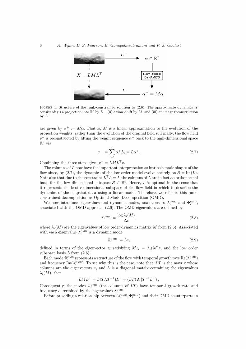
Figure 1. Structure of the rank-constrained solution to (2.6). The approximate dynamics Xconsist of: (i) a projection into Rr by L>; (ii) a time-shift by M ; and (iii) an image reconstructionby L.

are given by α+ := Mα. That is, M is a linear approximation to the evolution of theprojection weights, rather than the evolution of the original field v. Finally, the flow fieldv+ is reconstructed by lifting the weight sequence α+ back to the high-dimensional spaceRp via

v+ :=

r∑i=1

α+i Li = Lα+. (2.7)

Combining the three steps gives v+ = LML>v.The columns of L now have the important interpretation as intrinsic mode shapes of the

flow since, by (2.7), the dynamics of the low order model evolve entirely on S = Im(L).Note also that due to the constraint L>L = I, the columns of L are in fact an orthonormalbasis for the low dimensional subspace S ⊂ Rp. Hence, L is optimal in the sense thatit represents the best r-dimensional subspace of the flow field in which to describe thedynamics of the snapshot data using a linear model. Therefore, we refer to this rank-constrained decomposition as Optimal Mode Decomposition (OMD).

We now introduce eigenvalues and dynamic modes, analogous to λDMDi and ΦDMD

i ,associated with the OMD approach (2.6). The OMD eigenvalues are defined by

λOMD

i :=log λi(M)

∆t, (2.8)

where λi(M) are the eigenvalues of low order dynamics matrix M from (2.6). Associatedwith each eigenvalue λOMD

i is a dynamic mode

ΦOMD

i := Lzi (2.9)

defined in terms of the eigenvector zi satisfying Mzi = λi(M)zi and the low ordersubspace basis L from (2.6).

Each mode ΦOMDi represents a structure of the flow with temporal growth rate Re(λOMD

i )and frequency Im(λOMD

i ). To see why this is the case, note that if T is the matrix whosecolumns are the eigenvectors zi and Λ is a diagonal matrix containing the eigenvaluesλi(M), then

LML> = L(TΛT−1)L> = (LT ) Λ(T−1L>

).

Consequently, the modes ΦOMDi (the columns of LT ) have temporal growth rate and

frequency determined by the eigenvalues λOMDi .

Before providing a relationship between (λOMDi ,ΦOMD

i ) and their DMD counterparts in


section 2.4, we first emphasise the structure inherent in (2.6) by considering the problemof extracting dynamic information from a simple sinusoidal flow.

2.3. Example: Mode shapes and dynamics for a sinusoidal flow

In this section, it is shown that the dynamics of the sinusoidal flow

f(x, t) = sin (2πx− ωt)eγt (2.10)

can be represented naturally by a model of the form X = LML>, motivating the OMDmethod (2.6). Furthermore, the eigenvalues associated with the OMD method are shownto be λOMD

i = γ ± iω, meaning that the temporal dynamics of the flow can be exactlyidentified by solving (2.6).

Assume that data is sampled from (2.10) over a spatial window 0 = x1 < x2 <· · · < xp = 1 of p equally spaced points in [0, 1]. For a chosen time-step ∆t, N pairs(ui, u

+i )Ni=1 of flow snapshots are recorded in the form (2.1). For this simple example, the

two components L and M of the low order model can be explicitly constructed.(i) low dimensional subspace basis L: The flow dynamics can be separated into spatial

mode shapes and temporal weighting functions as

f(x, t) = a1(t)φ2(x) + a2(t)φ2(x) (2.11)

where a1(t) := − sin(ωt)eγt, a2(t) := cos(ωt)eγt and φ1(x) := cos (2πx), φ2(x) := sin (2πx).The snapshots ui, u

+i can therefore also be decomposed as

ui = a1(ti)v1 + a2(ti)v2, u+i = a1(ti + ∆t)v1 + a2(ti + ∆t)v2 (2.12)

for vectors v1, v2 ∈ Rp consisting of the values of φ1, φ2 at the points of the chosen spatialwindow,

v1 :=[φ1(x1) . . . φ1(xp)

]>, v2 :=

[φ2(x1) . . . φ2(xp)

]>.

The vectors v1, v2 therefore represent intrinsic mode shapes with which the observedsnapshot data can be described, and their span S := sp(v1, v2) ⊂ Rp is an appropriatelow dimensional subspace in which to identify the snapshot dynamics. This subspace canbe represented as the image of the matrix

L :=

↑ ↑v1/c v2/c↓ ↓

∈ Rp×2, (2.13)

where c := ‖v1‖2 = ‖v2‖2. Furthermore, since v1, v2 are orthogonal, the constraint L>L =I appearing in (2.6) is satisfied.

(ii) low order dynamics M : By (2.12), the flow dynamics depend entirely on the weightfunctions a1(t), a2(t) which satisfy

d

dt

[a1(t)a2(t)

]= eγt

[−γ sin (ωt)− ω cos (ωt)γ cos (ωt)− ω sin (ωt)

]=

(γ −ωω γ

)[a1(t)a2(t)

].

Since we want M to represent the evolution of the weights over ∆t, we obtain[a1(ti + ∆t)a2(ti + ∆t)

]= M

[a1(ti)a2(ti)

], M := e

(γ −ωω γ

)∆t.

Combining the above expression for M with (2.12) and (2.13), the relation betweeneach snapshot pair (ui, u

+i ) can be written simply as

u+i =

[v1 v2

] [a1(ti + ∆t)a2(ti + ∆t)

]=[v1 v2

]M

[a1(ti)a2(ti)

]= LML>ui.


which is the form of the dynamics in (2.6). Finally, notice that the rank constrainedeigenvalues λOMD given by (2.8) are the eigenvalues γ ± iω of(

λ −ωω λ

).

Hence, the temporal growth rate γ and frequency ω of the flow (2.10) are exactly identifiedby solving the OMD optimisation (2.6).

Since the underlying dynamics of the flow (2.10) are linear and noise-free, both theDMD and OMD methods will theoretically be able to exactly extract the eigenvalue in-formation. In section 5, the performance of both techniques are analysed for this examplewhen the snapshot data is corrupted with Gaussian noise. In the presence of noise, nei-ther method is able to exactly identify the true system eigenvalues. However, the OMDmethod (2.6) is shown to consistently outperform DMD in this case.

2.4. Relationship between DMD and OMD

Dynamic mode decomposition (2.3) is a restricted case of the optimal mode decomposi-tion (2.6). To see this, suppose that instead of optimising (2.6) over both variables, weassume that L is fixed and that the optimisation is performed over the single variableM . In other words, a low dimensional subspace of the flow field data is selected a-prioriand we search only for the best dynamical representation of the flow on that subspace.Since the best dynamics will depend on the particular subspace chosen, we denote thesolution of this restricted optimisation problem by M∗(L).

It is in fact possible to find an analytical expression for M∗(L) be equating the partialderivative

∂∥∥A− LML>B

∥∥2

∂M= 2

[−L>BA>L+ L>BB>LM>

]to zero, which implies that

M∗(L) := L>AB>L(L>BB>L

)−1. (2.14)

Now consider the particular case when L is fixed to be the first r columns of U , whereB = UΣV > is the compact singular value decomposition of B. In other words, the lowdimensional subspace represented by L is fixed to be an r-dimensional POD basis. Underthis restriction (2.14) becomes

M∗(U) = U>AB>U(U>BB>U

)−1= U>AV Σ−1 = S. (2.15)

Recalling that S is the matrix from (2.5) used in the DMD construction, it is now clearthat if L = U then λOMD

i = λDMDi and ΦOMD

i = ΦDMDi .

Consequently, DMD can be calculated as a special case of the OMD optimisation prob-lem (2.6). Furthermore, this relation implies that DMD can be interpreted as producinglow order dynamics which are a projection of the flow onto a POD-subspace, followed bya time-step governed by S. Viewed in this way as a rank-constrained optimisation of theform (2.6), the structural components of DMD are summarised in table 1.

It is now apparent that the DMD method is restrictive in the sense that the projectionis onto a fixed POD subspace. Since POD modes, especially in the case of randomlysampled data, do not intrinsically contain any dynamical information about the flow, itis not clear that L = U is the optimal choice of low dimensional subspace basis. Indeed,the restriction to a fixed basis in DMD can result in significant underperformance ofDMD in some cases. We give such an example in Appendix B. This motivates solving


DMD OMD

Low order subspace basis U L

Low order dynamics S M

Eigenvalues λDMDi = 1

∆tlog λi(S) λOMD

i = 1∆t

log λi(M)

Dynamic Modes ΦDMDi = Uyi ΦOMD

i = Lzi

Table 1. Structural components of the DMD and OMD flow models. When L = U the OMDmethod is equivalent to DMD.

(2.6) in which both the subspace represented by L and the dynamics M are searched forsimultaneously.

The difficulty in solving (2.6) is that the problem is non-convex. Our approach tothe problem is to use techniques from matrix manifold theory (Absil et al. 2008) whichare employed in the Section 4 to construct a method, Algorithm 1, to solve the OMDproblem (2.6).

3. Koopman Modes

Before proceeding to the numerical solution of the OMD problem (2.6), we explain therelation between OMD, DMD, and a related identification method in (Chen et al. 2012)referred to as ‘optimized DMD’ or opt-DMD in the context of the Koopman modes andeigenvalues of the underlying fluid system.

3.1. A Koopman mode interpretation of OMD

An introduction to Koopman modes, and their relation to DMD, is given in (Rowleyet al. 2009; Mezic 2013) and we therefore present only a brief summary here.

Suppose that the underlying velocity field is represented by an element z of a manifoldZ and evolves over a time-step ∆t to a new state z+ ∈ Z via the dynamical systemz+ = F (z). The Koopman (or composition) operator C is defined to act on the space ofone-dimensional observables† γ : Z → C via the composition formula

Cγ := γ F.Thus, Cγ : Z → C is itself an observable on Z with (Cγ)(z) = γ(F (z)) = γ(z+). Since Cis a linear operator, we may assume that it has an infinite basis of linearly independenteigenfunctions φCi : Z → C and associated eigenvalues λCi .

To consider data arising from experiments or simulations in fluid mechanics, it isconvenient to work with a vector-valued observable g : Z → Cp where, for example, eachcomponent of g(z) represents the velocity at a particular point in the instantaneous flowfield z. A standard assumption is that there exist vectors vKj ∈ Cp such that

g(z) =

∞∑j=1

vKj φCj (z). (3.1)

That is, it is assumed that each of the components of g lies in the span of the Koopman

† An observable is simply a scalar-valued function on the space Z. Since DMD and OMDmodes are in general complex, it is convenient to work with complex-valued observables even ifthe underlying data are real.


eigenfunctions φCj . Following (Budisic et al. 2012), define the space of all such observ-

ables by Fp. The vectors vKj are referred to as the Koopman modes of the mapping F

corresponding to the observable g. Since each φCj is an eigenfunction of C,

g(z+) =

∞∑j=1

vKj (CφCj )(z) =

∞∑j=1

vKj λCj φ

Cj (z). (3.2)

The compelling aspect of this analysis is that the above equality is exact and that the(nonlinear) evolution g(z) 7→ g(z+) of the observable can be described in terms of theeigenvalues and eigenfunctions of the (linear) Koopman operator. Furthermore, (3.2)allows a natural extension of the Koopman operator to act on such a vector-valuedobservable g = (g1, . . . , gp)

> ∈ Fp via

(Cg)(z) :=

∞∑j=1

vKj (CφCj )(z) =

(Cg1)(z)...

(Cgp)(z)

= g(z+), z ∈ Z. (3.3)

Now, suppose that the data ensemble arises in terms of an observable g such that(uj , u

+j ) = (g(zj), g(z+

j )). Then, using (3.3), the OMD optimization problem (2.6) canbe written in component form as

minL,M

N∑j=1

∥∥(Cg)(zj)− (LML>g)(zj)∥∥2

2, (3.4)

where the observable LML>g : Z → Cp is defined by (LML>g)(z) := LML>g(z).Therefore, given the data ensemble arising from an observable g ∈ Fp, OMD can bethough of as providing the optimal (in a least-squares sense) approximation to the Koop-man operator by a finite-rank operator of the form LML> : Fp → Fp.

We now explain the nature of the approximation that the OMD modes ΦOMDi and

eigenvalues λOMDi provide to the Koopman modes vKj and eigenvalues λCj . For the re-

mainder of this section it will be assumed that the data ensemble is sequential in thesense that u+

i = ui+1, i.e.,

B = (u1 | . . . |uN ) =(g(z1) | . . . | (CN−1g)(z1)

)A = (u2 | . . . |uN+1) =

((Cg)(z1) | . . . | (CNg)(z1)

) (3.5)

where z1 ∈ Z is the initial point of the underlying flow from which the data was sampled.

Now, consider decision variables L ∈ Rp×r and M ∈ Rr×r appearing in the OMDproblem (2.6). Assume M is diagonalizable as M = TΛT−1, define

V := B>L(L>BB>L)−1 ∈ RN×r

and recall that, by (2.9), the OMD modes ΦOMDi are the columns of LT . Note also that

the matrix V appears in (2.14) as a result of optimizing the OMD residual over M for afixed choice of basis L. A consequence is that an optimal solution pair L,M necessarilysatisfies

M = L>AV. (3.6)

This choice of M is intrinsically linked to the approximation that OMD modes andeigenvalues provide to the system’s Koopman modes and eigenvalues. To see why, consider


the observables ΦLi : Z → Cp defined by

ΦLi (z) :=

N∑j=1

vjiLL>g(F j−1(z)), (3.7)

where (vij)N ri=1 j=1 = VT and F is the mapping describing the evolution of the underlying

fluid system over one timestep ∆t. Using (3.5) it can be seen that ΦLi (z1) ∈ Cp is theith column of the matrix LL>BVT . Furthermore, since LL>BVT = LT it follows from(2.9) that ΦLi (z1) = ΦOMD

i . In other words, the OMD modes are equal to the values ofthe observables ΦLi at the initial point z1 ∈ Z of the underlying flow from which the datawas sampled.

Now, the value of each observable (CΦLi )(·) at the point z1 can be calculated using therelation ((

CΦL1)

(z1)∣∣ . . . ∣∣ (CΦLr

)(z1)

)= (LT )Λ + L(L>AV −M)T (3.8)

which is proven in theorem 2 of appendix A. Therefore, if L,M are optimal decisionvariables for OMD then (3.6) implies that

(CΦLi )(z1) = λOMD

i ΦLi (z1) = λOMD

i ΦOMD

i . (3.9)

Hence, the observables ΦLi (·) behave like vector-valued eigenfunctions of the Koopmanoperator with eigenvalues λOMD

i at the point z1 and, furthermore, are equal to the OMDmodes at that point: ΦLi (z1) = ΦOMD

i . In this sense, the OMD eigenvalues approximate asubset of the eigenvalues of the Koopman operator.†

We now link the OMD modes ΦOMDi with the Koopman modes vKi . Since C : Fp →

Fp is linear, we assume it has a basis of vector-valued eigenfunctions ΦCi ∈ Fp. Byassumption g ∈ Fp and, therefore, there exist scalars αi ∈ C such that

g(z) =

∞∑i=1

αiΦCi (z). (3.10)

The interpretation of (3.9) is now that (λOMDi ,ΦLi ) approximates the behavior of a true

eigenvalue-eigenfunction pair (λCj ,ΦCj ) at the point z1 ∈ Z. Assuming that the eigenvalue

λCj is simple with respect to the Koopman operator acting on scalar-valued observables,

lemma 1 of appendix A implies that ΦCj = wjφCj for some wj ∈ Cp. Using this relation to

expand (3.10) in terms of the scalar-valued eigenfunctions φCj , comparing the expression

to (3.1) and invoking linear independence implies that wjαj = vKj . Hence,

ΦOMD

i = ΦLi (z1) ≈ ΦCj (z1) = vKj(α−1j φCj (z1)

). (3.11)

In this sense each OMD mode ΦOMDi approximates a Koopman mode vKj , up to a multi-

plicative scalar.Interestingly, it is clear from (3.8) that equality holds in (3.9) for any decision variables

L,M satisfying (3.6). In other words, fixing L in (3.4) then optimizing over M only canbe interpreted as providing an approximation to the Koopman eigenvalues and modesfor any L. The particular case when L is fixed equal to U therefore provides a Koopmanmode interpretation of DMD‡. On the other hand OMD searches over all pairs L,M for

† It is shown in lemma 1 that the eigenvalues of C : Fp → Fp are the eigenvalues λCj of the

Koopman operator acting on scalar-valued observables.‡ The motivation for DMD in the literature is a slight modification of this argument. For

the DMD case when L is fixed to be U , because UU>g(zi) = g(zi) one may instead define the


which equality holds in (3.9) to obtain the variables which provide the ‘optimal’ (in theleast-squares sense of (3.4)) approximation to the Koopman operator of the finite-rankform LML> : Fp → Fp.

It is important to note that (3.9) does not imply that ΦLi is an eigenfunction of C,merely that ΦLi behaves like an eigenfunction at the single point z1 ∈ Z. Furthermore,(3.9) does not quantify the quality of the approximation that the observables ΦLi provideto the true Koopman eigenfunctions ΦCi . Essentially, this is due to the fact that we onlyhave information concerning a single point z1 ∈ Z of the underlying fluid system. Forthis reason, we emphasise that it is not currently possible to say whether either DMD orOMD provides a better approximation to the true Koopman modes vKj and eigenvalues

λCj .

3.2. Optimized Dynamic Mode Decomposition

Koopman modes also provide the motivation for the recently proposed Optimized Dy-namic Mode Decomposition (opt-DMD) algorithm in Chen et al. (2012). To calculateopt-DMD, the following optimization problem is solved:

minV,T

‖B − V T‖2Fs.t. V ∈ Rp×r,

T =

1 λ1 λ2

1 . . . λN−11

1 λ2 λ22 . . . λN−1

2...

......

...1 λr λ2

r . . . λN−1r

, some λi ∈ R.

(3.12)

The resulting mode shapes Φopt-DMD

i are the columns of the optimal variable V witheigenvalues λopt-DMD

i given by the corresponding entries of the optimal matrix T . The linkbetween opt-DMD and OMD is given by the fact, proven in theorem 3 of appendix A,that (3.12) is equivalent to

minL,M,ξ1

N∑i=1

‖ui − (LML>)i−1ξ1‖22

s.t. L>L = I, M diagonalizable, ξ1 ∈ Im(L).

(3.13)

Thus, opt-DMD can be thought of as searching for the best (in a least-squares sense)linear trajectory ξ1, Xξ1, . . . , XN−1ξ1 to fit the data u1, . . . , uN, under the restric-tions: (i) the linear process has the low-order form X = LML>; and (ii) the initial valueξ1 of the trajectory lies in the subspace spanned by L.

Note that while the DMD and OMD methods do not actually require a sequentialdata ensemble to work, opt-DMD does require sequential data. The reader will alsoobserve that the objective function in (3.12) is an N th order polynomial function of theparameters λi, where N is the number of data samples. As noted in Chen et al. (2012),the resulting optimization problem is very difficult to solve, and the authors proposed

observables ΦUi without the projection term UU>. The right-hand-side of (3.8) corresponding

to this choice of observables is then UTΛ + (A − UMU>B)VT . Since DMD selects M = Sto minimize A − UMU>B, a similar argument to the above imples that DMD approximatesthe Koopman eigenvalues and modes, albeit without equality in (3.9). Note that the resulting

residual A−USU>B is equal to the “re>” term in (Rowley et al. 2009, Equation (3.12)) while

(A− USU>B)VT is equal to the “ηre>V −1” term in (Budisic et al. 2012, Equation (57)).


a randomized solution approach based on simulated annealing. In contrast, we showin section 4 that a solution to the OMD optimization problem (2.6) can be computedusing a standard gradient-based algorithm which require only standard linear algebraicoperations, is deterministic and is guaranteed to converge.

The original Koopman-mode motivation for opt-DMD is explained by the fact that theVandermonde structure of T in (3.12) implies that the data sequence can be representedas

ui =

r∑j=1

(λopt-DMD

j )i−1Φopt-DMD

j + ri (3.14)

where ri are components of the associated optimization residual. On the other hand, arecursive application of (3.2) implies that each ui can alternatively be written in termsof the true Koopman modes and eigenvalues as

ui =

∞∑j=1

vKj (λCj )i−1φCj (z1). (3.15)

Since (3.14) resembles a finite truncation of (3.15), it is argued in Chen et al. (2012) thatthe opt-DMD modes and eigenvalues approximate a subset of the Koopman modes andeigenvalues. Again, there is an unquantified approximation involved in this argument,since even small residuals ri do not guarantee that the identified modes and eigenvaluesare close to a subset of the true Koopman modes and eigenvalues.

3.3. Optimal Koopman mode identification?

We end this section by briefly reiterating that, at the current state of the literature,it is not clear which of DMD, OMD or opt-DMD produces the best approximation tothe Koopman modes and eigenvalues. This is since the arguments used to relate theKoopman modes to the modes produced by each algorithm all require an approximationstep, as described in sections 3.1 and 3.2, and the quality of the approximation cannotbe formally quantified for any of the methods.

However, since OMD (and DMD when L is fixed to be U) seeks to minimize theleast-squares sum of the residuals

(Cg)(zj)− (LML>g)(zj),

it can be thought of as providing a finite rank approximation LML> : Fp → Fp to theKoopman operator. On the other hand, opt-DMD seeks to minimize the least-squaressum of residuals

(Cj−1g)(z1)− (LML>)j−1ξ1

for some ξ1 ∈ Im(L). In this case, the direct link between C and LML> is less obviousand, instead, the similarity of the sums (3.14) and (3.15) motivates the link betweenopt-DMD and the Koopman operator. To our knowledge it is therefore an importantopen problem to formally quantify the approximation that each of the three methodsprovides to the true Koopman modes and eigenvalues. This will form the basis of futureresearch.

4. Solution to the OMD minimisation problem

The aim is to construct optimal variables L and M which minimize the norm in (2.6).For a fixed L, the minimum M∗(L) over the variable M is given by (2.14). Hence,


(2.6) can be solved by substituting the expression for M∗(L) into the norm in (2.6) andoptimising over the single variable L. Performing this substitution gives∥∥A− LM∗(L)L>B

∥∥2=∥∥A− LL>AQ(L)

∥∥2= ‖A‖2 −

∥∥L>AQ(L)∥∥2,

where Q(L) := B>L(L>BB>L

)−1L>B is an orthogonal projection defined in terms

of L. Consequently, the two-variable minimisation problem (2.6) is equivalent to thesingle-variable maximisation problem

max g(L) :=∥∥L>AQ(L)

∥∥2

s.t. L ∈ Rp×r, L>L = I,

Q(L) = B>L(L>BB>L

)−1L>B.

(4.1)

If a maximiser L∗ to (4.1) can be found, it provides a solution pair (L∗,M∗(L∗)) to (2.6),with M∗(L∗) given by (2.14). Algorithm 1, stated below, provides an iterative methodfor solving (4.1). It is a conjugate-gradient based algorithm, tailored to exploit intrinsicproperties of (4.1) by using tools from matrix manifold theory.

The fundamental property of (4.1) which must be utilized by any gradient-based al-gorithm is that it is an optimisation over r-dimensional subspaces of Rp, rather thansimply a matrix-valued optimisation. To see why this is true, note first that due to theconstraint L>L = I, each feasible variable L ∈ Rp×r represents an orthonormal basisfor the subspace Im(L) ⊂ Rp. Hence, if L1, L2 are two variables representing the samesubspace then there exists an orthogonal transformation P ∈ Rr×r such that L1 = L2P .Consequently,

g(L1) = f(L2P ) = ‖P>L>2 AQ(L2P )‖ = ‖L>2 AQ(L2)‖ = g(L2),

which implies that it is only the subspace represented by the variable L which determinesthe value g. The search for an optimal value of g must therefore be performed over themanifold of r-dimensional subspaces of Rp, known as the Grassman manifold Gr,p.

Each element of the Grassman manifold Gr,p, i.e. each r-dimensional subspace S ⊂ Rp,is represented by any matrix with orthogonal columns which span that subspace S. Forexample, elements of the manifold G2,3 depicted in figure 2 are planes in R3. Each planecan be represented by any matrix L ∈ R2×3 whose columns are a pair of orthogonalunit vectors in that plane, as shown in figure 2 (a). An effective search algorithm over aGrassman manifold must take into account this fact that each point in the manifold isrepresented by infinitely many matrices. In particular, search directions will be chosenalong geodesics of the manifold, which represent the shortest distance between two givensubspaces, while the search direction itself is determined by the gradient∇g at the currentpoint on the manifold.

In (Edelman et al. 1998), the following formulae are given for the gradient and geodesiccurves on a Grassman manifold. Given an element of Gr,p represented by a matrix L0 ∈Rr×p, the gradient of a function g at L0 is given by

∇g = (I − L0L>0 )gL0

,

where gL0:= ∂g

∂L (L0). The geodesic passing through L0 in the direction ∇g is given bythe parameterized formula

L0(t) = L0V cos (Σt)V > + U sin (Σt)V >, t ∈ [0, 1],

where∇g = UΣV > is the compact singular value decomposition of∇f . These expressionsare used in algorithm 1 to provide a solution to (4.1).


(a) (b)

Figure 2. The Grassman manifold G2,3 (a) Variables for (4.1) are matrices whose columnsare orthogonal elements of the unit sphere. In the case depicted, variables L1, L2 ∈ R3×2 havecolumns as solid and dotted unit vectors, respectively. Both matrices represent the same subspaceand hence the same element of G2,3. Furthermore, g(L1) = g(L2). (b) A sequence of elementsof G2,3, representing ‘subspace variables’ of (4.1).

Algorithm 1 Conjugate gradient algorithm for solution of (4.1)

1: set initial L0 ∈ Rp×r satisfying L>0 L0 = I.2: compute initial gradient G0 := (I − L0L

>0 )gL0

and search direction H0 := −G0

3: repeat for k = 0, 1, 2, . . . 4: compute minimiser tmin ∈ [0, 1] of g(Lk(t)) over the geodesic curve

Lk(t) := LkV cos (Σt)V > + U sin (Σt)V >, t ∈ [0, 1],

in direction Hk = UΣV >

5: update subspace basis Lk+1 := Lk(tmin)6: update gradient

Gk+1 := (I − Lk+1L>k+1)gLk+1

7: update (conjugate-gradient) search direction

Hk+1 := Gk+1 + ∆k+1

8: until g(Lk+1)− g(Lk) < tolerance9: return Optimal low order subspace basis Lk+1 and dynamics M(Lk+1).

Algorithm 1 is described in Edelman et al. (1998) and is included here for completeness.With respect to the particular problem (4.1), specific expressions for the partial derivativegL0

:= ∂g∂L (L0) and the conjugate-gradient correction ∆k+1 are given in appendix C. It

should be noted that other algorithmic techniques, such as Newton’s method, have beendeveloped for subspace-valued optimisation and may therefore also be applied to (4.1).The reader is referred to (Edelman et al. 1998; Goulart et al. 2012) for more details†.

4.1. Computational performance

We now compare the computational performance of OMD with respect to DMD. Eachalgorithm is applied to a data ensembles taken from an experimental data set of velocitymeasurements for flow over a backward facing step. The experiment is described in detailin section 6. Each snapshot contains velocity data at p = 15600 pixels and data ensembles

† A MATLAB implementation of algorithm 1 and its application to the example of Section 5is available at http://control.ee.ethz.ch/~goularpa/omd/.


r = 10 r = 20 r = 50 r = 100

N = 100 0.94 (0.20) 4.15 (0.20) 24.65 (0.20) 7.83 (0.20)

N = 200 2.56 (0.50) 8.04 (0.50) 11.45 (0.50) 28.00 (0.50)

N = 500 4.17 (1.82) 11.40 (1.82) 39.90 (1.82) 113.65 (1.82)

N = 1000 9.15 (6.20) 16.72 (6.20) 69.49 (6.20) 157.00 (6.20)

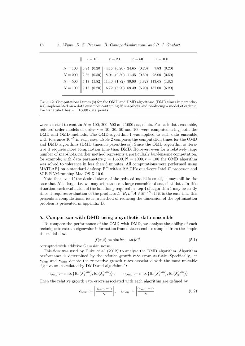
Table 2. Computational times (s) for the OMD and DMD algorithms (DMD times in parenthe-ses) implemented on a data ensemble containing N snapshots and producing a model of order r.Each snapshot has p = 15600 data points.

were selected to contain N = 100, 200, 500 and 1000 snapshots. For each data ensemble,reduced order models of order r = 10, 20, 50 and 100 were computed using both theDMD and OMD methods. The OMD algorithm 1 was applied to each data ensemblewith tolerance 10−5 in each case. Table 2 compares the computation times for the OMDand DMD algorithms (DMD times in parentheses). Since the OMD algorithm is itera-tive it requires more computation time than DMD. However, even for a relatively largenumber of snapshots, neither method represents a particularly burdensome computation;for example, with data parameters p = 15600, N = 1000, r = 100 the OMD algorithmwas solved to tolerance in less than 3 minutes. All computations were performed usingMATLAB† on a standard desktop PC with a 2.2 GHz quad-core Intel i7 processor and8GB RAM running Mac OS X 10.6.

Note that even if the desired size r of the reduced model is small, it may still be thecase that N is large, i.e. we may wish to use a large ensemble of snapshot data. In thissituation, each evaluation of the function g required in step 4 of algorithm 1 may be costlysince it requires evaluation of the products L>B,L>A ∈ Rr×N . If it is the case that thispresents a computational issue, a method of reducing the dimension of the optimizationproblem is presented in appendix D.

5. Comparison with DMD using a synthetic data ensemble

To compare the performance of the OMD with DMD, we analyse the ability of eachtechnique to extract eigenvalue information from data ensembles sampled from the simplesinusoidal flow

f(x, t) := sin(kx− ωt)eγt, (5.1)

corrupted with additive Gaussian noise.This flow was used by Duke et al. (2012) to analyse the DMD algorithm. Algorithm

performance is determined by the relative growth rate error statistic. Specifically, letγDMD and γOMD denote the respective growth rates associated with the most unstableeigenvalues calculated by DMD and algorithm 1:

γDMD := max Re(λDMD

1 ),Re(λDMD

2 ) , γOMD := max Re(λOMD

1 ),Re(λOMD

2 )Then the relative growth rate errors associated with each algorithm are defined by

εDMD :=

∣∣∣∣γDMD − γγ

∣∣∣∣ , εOMD :=

∣∣∣∣γOMD − γγ

∣∣∣∣ . (5.2)


Thus εDMD and εOMD measure the quality of approximation that the extracted low orderdynamics provide to the true temporal growth rate γ.

Relative growth rate errors were calculated using data simulated from (5.1). Growthrate and spatial frequency were chosen to be γ = k = 1, while temporal frequency wasvaried over the range ω ∈ [0.6, 1.6]. The number of temporal snapshots was N = 50, takenat time intervals dt = π/100, while p = 200 spatial samples were taken at intervals dx =π/100. After arranging snapshots into ‘before’ and ‘after’ matrices A,B ∈ Rp×N , thedata was corrupted by adding zero-mean Gaussian noise with covariance σ2 ∈ [0.052, 1].At each covariance and temporal frequency pair (σ2, ω) ∈ [0.052, 1]× [0.6, 1.6], 103 dataensembles were created and both DMD and algorithm 1 were applied to each simulationensemble. Calculation of the DMD eigenvalues was performed using the method describedin Duke et al. (2012) with a rank-reduction ratio of 10−1. A rank reduction ratio of 10−1

refers to the truncation of the matrix Σ of singular values used in the calculation of DMD(see section 2.1) to contain only those values within 10% of the most energetic singularvalue.

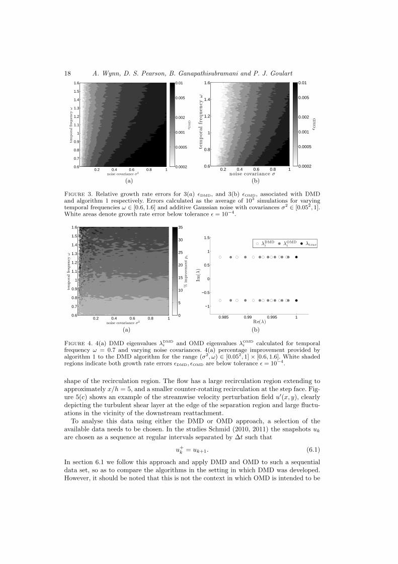
Figure 3(a) depicts the growth rate errors εDMD and figure 3(b) the errors εOMD. Forboth algorithms, performance improves as temporal frequency increases, since more wave-lengths are contained in the data ensemble. Performance also improves as noise covari-ance decreases. However, it is apparent that for all temporal frequencies in the simulationrange, the error εOMD associated with algorithm 1 is lower than the error εDMD associatedwith DMD. Hence, algorithm 1 provides an improvement over DMD for the considereddata parameters.

To analyze this performance advantage further, the percentage improvement

pε := 100% · (εDMD − εOMD)/εDMD

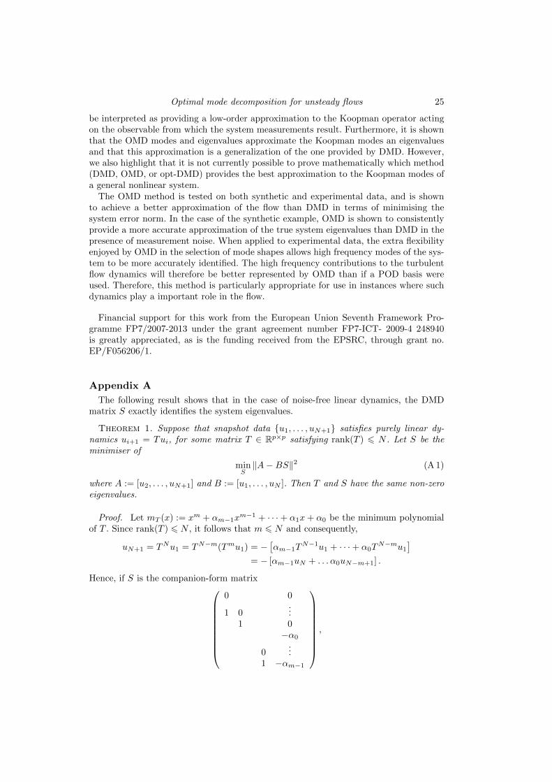
is plotted in figure 4(a). The horizontal banded structure implies that the percentageimprovement provided by algorithm 1 over DMD is dependent on temporal frequency asopposed to noise covariance. Furthermore, pε increases as ω increases.

Figure 4(b) shows the DMD eigenvalues λDMDi and OMD eigenvalues λOMD

i calculatedfor a fixed temporal frequency ω = 0.7 and varying noise covariances σ2 ∈ [0.352, 1]. Foreach noise covariance level, the pair of eigenvalues calculated by each of the algorithmsis plotted. As noise covariance increases, both algorithms produce eigenvalues which areincreasingly more stable (to the left of the figure) than the true eigenvalues λtrue =1 ± 0.7i. However, the OMD eigenvalue pairs are consistently closer to the true systemeigenvalues than the DMD eigenvalues and hence provide a more accurate approximationof the relative growth rate error.

6. Analysis of the backward-facing step

A demonstration of the OMD algorithm on an experimental data set is now presented.The data set is of a low-speed turbulent boundary layer flow over a backward-facingstep, measured using two-dimensional time-resolved Particle Image Velocimetry (PIV).The step, of height h = 30mm, spans the full width of the wind tunnel and is down-stream of a turbulent boundary layer of thickness δ = 44mm, with a free stream velocityof 6m/s. The PIV field of view is in the wall-normal plane parallel to the streamwise flowas schematically depicted in figure 5(a). The data is acquired at a frequency Fs = 8000Hzfor approximately 4 seconds, resulting in 31606 images, from which 31605 vector fieldswere calculated. The processing was done using a 16 × 16 pixel window with 50% over-lap, providing vector fields with a spatial resolution of approximately 1.1mm. Figure 5(b)shows contours of the mean flow field, with streamlines overlaid to illustrate the size and


noise covariance σ2

temporalfrequency

ω

0.2 0.4 0.6 0.8 10.6

0.7

0.8

0.9

1

1.1

1.2

1.3

1.4

1.5

1.6

ε DM

D

0.0002

0.0005

0.001

0.002

0.005

0.01

(a)noise covariance σ

temporalfrequencyω

0.2 0.4 0.6 0.8 10.6

0.8

1

1.2

1.4

1.6

εOMD

0.0002

0.0005

0.001

0.002

0.005

0.01

(b)

Figure 3. Relative growth rate errors for 3(a) εDMD, and 3(b) εOMD, associated with DMDand algorithm 1 respectively. Errors calculated as the average of 103 simulations for varyingtemporal frequencies ω ∈ [0.6, 1.6] and additive Gaussian noise with covariances σ2 ∈ [0.052, 1].White areas denote growth rate error below tolerance ε = 10−4.

noise covariance σ2

temporalfrequency

ω

0.2 0.4 0.6 0.8 10.6

0.7

0.8

0.9

1

1.1

1.2

1.3

1.4

1.5

1.6

%im

provementpε

0

5

10

15

20

25

30

35

(a)

0.985 0.99 0.995 1

−1

−0.5

0

0.5

1

1.5

Re(λ)

Im(λ

)

λDMDi

λOMDi

λtrue

(b)

Figure 4. 4(a) DMD eigenvalues λDMDi and OMD eigenvalues λOMD

i calculated for temporalfrequency ω = 0.7 and varying noise covariances. 4(a) percentage improvement provided byalgorithm 1 to the DMD algorithm for the range (σ2, ω) ∈ [0.052, 1] × [0.6, 1.6]. White shadedregions indicate both growth rate errors εDMD, εOMD are below tolerance ε = 10−4.

shape of the recirculation region. The flow has a large recirculation region extending toapproximately x/h = 5, and a smaller counter-rotating recirculation at the step face. Fig-ure 5(c) shows an example of the streamwise velocity perturbation field u′(x, y), clearlydepicting the turbulent shear layer at the edge of the separation region and large fluctu-ations in the vicinity of the downstream reattachment.

To analyse this data using either the DMD or OMD approach, a selection of theavailable data needs to be chosen. In the studies Schmid (2010, 2011) the snapshots ukare chosen as a sequence at regular intervals separated by ∆t such that

u+k = uk+1. (6.1)

In section 6.1 we follow this approach and apply DMD and OMD to such a sequentialdata set, so as to compare the algorithms in the setting in which DMD was developed.However, it should be noted that this is not the context in which OMD is intended to be


PIV camera 1 field PIV camera 2 field

U∞δ

h

y/h

x/h0 54321

(a)

x/h

y/h

1 2 3 4 5

0.5

1

1.5

−0.2

0.0

0.2

0.4

0.6

0.8

1.0

(b)

x/h

y/h

1 2 3 4 5

0.5

1.0

1.5

−0.2

−0.1

0.0

0.1

0.2

(c)

Figure 5. 5(a) A schematic representation of the PIV field of view and coordinate system; 5(b)Contours of the mean streamwise velocity with selected mean streamlines; 5(c) An example ofa PIV u′ velocity field.

applied. For this reason, in section 6.2, the OMD algorithm is also applied to snapshotpairs (uk, u

+k ) sampled at irregular time instances tk.

There is no precise way of determining the best number of snapshots N and thetemporal separation ∆t of the snapshot pairs. Any appropriate selection is dependenton the amount, type and format of the data and the dynamics to be modelled. Dukeet al. (2012) calculated the relation between these parameters (among others) to theestimation error on the synthetic sinusoid (5.1). These results showed that, even for thissimple waveform, the dependency of the relative growth rate error ε on the choice ofmethod parameters is complex. They note in particular that error is sensitive to the datasignal-noise ratio and the resolution of the data sampling.

Measurement noise is quantified by the magnitude of noise floor of the velocity powerspectrum. Figure 6(a) shows the spectra for the present data at five different streamwisepositions and a noise floor at approximately 2000Hz is observed. This high frequencymeasurement noise is over three orders of magnitude lower than the dominant low fre-quencies and, for all analyses performed in this section, is removed using a low-passfilter.

The appropriate choice of ∆t needs to be made so that sufficient resolution is providedat the dominant frequencies modelled by the matrices S or M . As shown in section 2.2,these matrices do not describe the evolution of the velocity field uk 7→ u+

k , but ratherthat of the basis weights αi 7→ α+

i . Furthermore, in section 2.4 it was shown that the


101

102

103

10−8

10−7

10−6

10−5

10−4

10−3

f (Hz)

Φ(u

′ ,f)

[x/h, y/h]

2kHz Filter

f h/U∞

[1, 0.0][2, 0.9][3, 0.9][4, 0.9][5, 0.9]

10−1

100

101

(a)

100

101

102

103

0

1

2

3

4

5

6

f (Hz)f·Φ

(αi,f)

f h/U∞

α1,DMD

α2,DMD

α5,DMD

α10,DMD

α25,DMD

10−2

10−1

100

(b)

Figure 6. 6(a) The u′ power spectral density of the flow at 5 streamwise locations withlow-pass filter shown; 6(b) The pre-multiplied power spectra of the mode weights αi.

DMD basis is the POD modes and that αi,DMD are the POD weights. Since the PODbasis is readily calculated for any data set, and is also a suitable initial condition forOMD optimisation, inspecting the frequency content of αi,DMD also serves as a usefulguide to the choice of appropriate ∆t for the OMD method.

Figure 6(b) is the pre-multiplied power spectra for the POD weights αi(t) shownfor i = 1, 2, 5, 10, 25 over the full set of vector fields. The magnitude of the peakpower of each mode varies, with the higher modes dominated by higher frequencies.However, all modes contain very little frequency content above 200Hz and the mostdominant frequencies are typically closer to 10Hz. To achieve relative growth-rate errorsof εDMD < 0.1%, Duke et al. (2012) recommend that the dominant wavelength shouldcontain at least 40 samples. In addition, for a sequential data set, we require the totalnumber of snapshots to span several full periods of the dominant wavelength. For thesequential data case studied in section 6.1 these criteria are satisfied by setting N = 200and ∆t = 20/Fs, which provide 5 full periods of data with frequency 10Hz while keepingthe computation within the capability of a desktop computer.

6.1. Comparison between DMD and OMD for sequential data

The individual modes of the L basis calculated using algorithm 1 typically bear littleresemblance to those of the POD basis U used in DMD. However, since both bases arecomprised of mutually orthogonal basis functions, each basis remains invariant underan orthogonal transformation L 7→ LR. For the purposes of comparing the two, the Lmatrix can be transformed such that the modes are best aligned to the singular values ofB in the same manner as a POD basis (Goulart et al. 2012). This is achieved using thesingular value decomposition LTB = U ΣV T and setting R = U . All the following OMDresults have been transformed in this way.

For a data set of the sequential form (6.1), the estimated mode weights at each samplepoint tk

α+i,DMD

(tk) := Sαi,DMD(tk) ; α+i,OMD

(tk) := Mαi,OMD(tk) ,


−10

−5

0

5

α+ i

α+1,DMD α+

1,DMD

−10

−5

0

5

α+ i

α+1,OMD α+

1,OMD

−4

−2

0

2

4

α+ i

α+10,DMD α+

10,DMD

−4

−2

0

2

4

α+ i

α+10,OMD α+

10,OMD

0 0.05 0.1 0.15−2

−1

0

1

2

3

sample point (sec.)

α+ i

α+50,DMD α+

50,DMD

0 0.05 0.1 0.15−2

−1

0

1

2

3

sample point (sec.)

α+ i

α+50,OMD α+

50,OMD

Figure 7. Comparison of the actual mode weights, α+i , with those estimated over a single

time step, α+i , for both DMD and OMD analyses.

0 20 40 60 80 1000

1

2

3

4

5

6

ith mode

‖α+ i−

α+ i‖

DMDOMD

(a)

0 20 40 60 80 10050

60

70

80

90

100

110

120

130

rank(X)

‖A−

XB‖

DMDOMD

(b)

Figure 8. 8(a) The norm estimation error of α+ using the DMD and OMD analyses, for eachmode of a rank-100 system; 8(b) The norm system error for DMD and OMD analyses of systemswith varying rank.

can be compared directly to the actual values

α+i,DMD

(tk) = αi,DMD(tk+1) ; α+i,OMD

(tk) = αi,OMD(tk+1) ,

to demonstrate the single-point estimation capability of both methods. Figure 7 showsα+ and α+ for modes i = 1, 10, 50 on a system of rank 100 using each method. Theblack markers indicate the sample points tk with separation ∆t = 20/Fs.

The actual weights (black lines) of the POD modes α+i,DMD

and those of the transformed

L-basis α+i,OMD

are similar at low modes, but are different at the higher modes, for examplei = 50. This demonstrates that both methods use similar modes to describe the largestructures, but have found different modes to represent the high frequencies. This extra


freedom in mode shape selection allows OMD to produce dynamics which more accuratelycapture the evolution of the snapshot data.

In figure 7, it can be seen that, compared to DMD, the estimated weight sequence givenby OMD more accurately models the true weights of the snapshot data when projectedonto the identified low order subspace. Figure 8(a) highlights this by showing the normestimation error of each method for all 100 modes. The error of the OMD method isover 4 times lower than that of the DMD method across all modes. Figure 8(b) showsthis translates into a lower estimation error of the system ‖A − XB‖ as a whole. Thedifference in the error becomes larger as the system rank increases, meaning that theOMD algorithm performs proportionately better when the system has many modes. Thisis because, as shown in figure 7, OMD has the freedom to capture the high frequenciesto a greater accuracy than DMD. This is a major advantage in systems for which thehigh frequency (and often low energy) modes play a crucial role in the flow dynamics(Ma et al. 2011).

We now consider the modes and eigenvalues produced by the OMD and DMD al-gorithms. Subsets of the eigenvalues of S and M are plotted against the unit circle infigure 9 for (a) a rank-100, (b) a rank-150 and (c) a rank-200 mode approximation to theN = 200 mode sequential data ensemble. Figure 9(a) shows the eigenvalues correspond-ing to the rank-100 approximation analysed in figures 7 and 8. It can be seen that theOMD eigenvalues are concentrated in a narrower band than the DMD eigenvalues andare also closer to the unit circle, which corresponds to the right-shift trend observed forthe sinusoidal waveform in figure 4(b). With increasing rank of approximation, the abso-lute difference between the OMD and DMD eigenvalues can be seen to decrease in figures9(b)-9(c), although the shift trend is still clearly visible for the rank-150 approximationin figure 9(b).

In figures 9(d)-9(f) the OMD modes corresponding to the eigenvalues highlighted inblue in figure 9(a) are shown. Despite the fact that a lower rank system is used togenerate them, it is interesting to note that they represent similar spatial structuresto the fully converged DMD modes shown in figures 9(g)-9(i), which correspond to theeigenvalues highlighted in blue in figure 9(c). The Strouhal numbers St := fh/U∞ of thehighlighted OMD modes are 0, 0.452, 0.957, respectively, and those of the DMD modesare 0, 0.391, 1.005, respectively. We reserve comment on the physical interpretation of themode shapes until section 6.2.

As discussed in section 3, the DMD modes can be viewed as approximations of theunderlying Koopman modes of the system. The convergence of DMD and OMD modesfor a full-rank (r = 200, N = 200) approximation implies that, for this example, OMDand DMD both provide similar approximations to the Koopman modes in this case. Werestate, however, that it is not known which method produces the best approximation tothe Koopman modes of a general nonlinear system. When a lower-order approximationis used, OMD is nonetheless able to produce mode shapes representing similar spatialstructures to the fully converged DMD modes. We develop this idea in the followingsection by applying the OMD algorithm to an irregularly sampled data ensemble andshow that coherent mode shapes can be created by using models of significantly lowerrank than the dimension of the data ensemble.

6.2. OMD modes and eigenvalues for irregularly sampled data

The OMD algorithm is applied to a data ensemble (ui, u+i )Ni=1 containing N = 800

irregularly sampled snapshot pairs to create a rank r = 16 approximation. The factthat a only very low order approximating system is searched for makes the problemcomputationally feasible. Furthermore, using a large number of snapshots helps account


0.6 0.8 1 1.2

0

0.1

0.2

0.3

0.4

0.5

0.6

Real(λi)

Imag(λ

i)

λi(S)

λi(M)

(a)

0.6 0.8 1 1.2

0

0.1

0.2

0.3

0.4

0.5

0.6

Real(λi)

Imag(λ

i)

λi(S)

λi(M)

(b)

0.6 0.8 1 1.2

0

0.1

0.2

0.3

0.4

0.5

0.6

Real(λi)

Imag(λ

i)

λi(S)

λi(M)

(c)

(d) (e) (f)

(g) (h) (i)

Figure 9. (a)-(c) Eigenvalues of S (DMD) and M (OMD) calculated using an ensemble ofN = 200 sequential snapshots and with r = 100, 150, 200, respectively. In each case, the solidline is an arc of the unit circle. OMD modes corresponding to eigenvalues highlighted in blue in(a) are plotted as (d)-(f). DMD modes corresponding to eigenvalues highlighted blue in (c) areplotted (g)-(i).

for any measurement noise present in the data ensemble. The OMD algorithm produceseigenvalues of M in an arc-like pattern symmetric about the real axis, as shown in figure10(a). In comparison to the fully converged DMD and OMD eigenvalues in figure 9(c),which are distributed upon the entire unit circle and hence represent a wide frequencyrange, the arc of OMD eigenvalues in figure 10(a) corresponds to a set of relatively lowfrequency modes. The OMD eigenvalues λOMD

i = (∆t)−1 log λi(M) are also plotted infigure 10(b).

The OMD mode shapes can be seen to separate into two subsets; low frequency modeswith lighter damping in figures 10(c)-10(e) and more highly damped high-frequencymodes in figures 10(f)-10(h). The low frequency modes are linked to the behaviour ofthe recirculation region, shown schematically in figure 5(a). Mode (c) is a near-persistentstructure and resembles the modes 9(d) and 9(g) identified using the sequential dataensemble. Mode 10(d) has a region of recirculation near y = 0 between 2 6 x/h 6 4.5.In addition, it contains a larger area of flow in the free-stream direction indicating cou-pling between the behaviour of the recirculation region and the shear layer. Mode 10(e)contains a large region of flow in the freestream direction with a smaller region of re-versed flow between 2 6 x/h 6 3. This mode has similar spatial features to 9(e) and 9(h)although is has slightly lower frequency. Finally, modes 10(f)-10(h) contain successiveregions of low and high speeds in the shear layer that separates the recirculation regionfrom the freestream. These modes represent the instabilities and the roll up of the shear


−1 −0.5 0 0.5 1

−1

−0.5

0

0.5

1

Real(λi)

Imag(λ

i)

(a)

−400 −200 0 200 400−50

−40

−30

−20

−10

0(c)

(d)

(e)(f)

(g)

(h)

Imag(λi)

Real(λi)

(b)

(c) (d) (e)

(f) (g) (h)

Figure 10. The OMD modes for turbulent flow over a backstep. A low-order model withr = 16 modes is calculated using N = 800 snapshot pairs. OMD eigenvalues shown indiscrete (a) and continuous (b) time. Low-frequency modes (c)-(e) with Strouhal Num-bers St = 0.017, 0.188, 0.279 and high-frequency modes (f)-(h) with Strouhal numbersSt = 0.847, 1.1824, 1.527.

layer. It is interesting to note that the high frequency modes appear to be much moreconverged versions of the modes 9(f) and 9(i) identified from the sequential data ensem-ble. A possible explanation is that the low-order modelling capability of OMD allows theuse of a large number of snapshots and enables a better extraction of coherent structuresfrom the data ensemble.

7. Conclusions

A general method of approximating the dynamics of a high-dimensional non-linearfluid system using a linear system of chosen rank has been presented. The system isfirst projected onto an orthogonal basis of chosen rank. The linear evolution of the flowis calculated on the low-rank basis, before projecting the result back to the originaldimension. The choice of basis and the linear model are both variables in the optimisation,in which the error ‖A−XB‖ is minimised in the Frobenius norm.

It is shown that if the basis is chosen to be that of the system POD modes, andremains fixed during optimisation, then the DMD solution results. The present methodis therefore a generalisation of the DMD algorithm.

The relation of OMD to Koopman modes is discussed and it is shown that OMD can


be interpreted as providing a low-order approximation to the Koopman operator actingon the observable from which the system measurements result. Furthermore, it is shownthat the OMD modes and eigenvalues approximate the Koopman modes an eigenvaluesand that this approximation is a generalization of the one provided by DMD. However,we also highlight that it is not currently possible to prove mathematically which method(DMD, OMD, or opt-DMD) provides the best approximation to the Koopman modes ofa general nonlinear system.

The OMD method is tested on both synthetic and experimental data, and is shownto achieve a better approximation of the flow than DMD in terms of minimising thesystem error norm. In the case of the synthetic example, OMD is shown to consistentlyprovide a more accurate approximation of the true system eigenvalues than DMD in thepresence of measurement noise. When applied to experimental data, the extra flexibilityenjoyed by OMD in the selection of mode shapes allows high frequency modes of the sys-tem to be more accurately identified. The high frequency contributions to the turbulentflow dynamics will therefore be better represented by OMD than if a POD basis wereused. Therefore, this method is particularly appropriate for use in instances where suchdynamics play a important role in the flow.

Financial support for this work from the European Union Seventh Framework Pro-gramme FP7/2007-2013 under the grant agreement number FP7-ICT- 2009-4 248940is greatly appreciated, as is the funding received from the EPSRC, through grant no.EP/F056206/1.

Appendix A

The following result shows that in the case of noise-free linear dynamics, the DMDmatrix S exactly identifies the system eigenvalues.

Theorem 1. Suppose that snapshot data u1, . . . , uN+1 satisfies purely linear dy-namics ui+1 = Tui, for some matrix T ∈ Rp×p satisfying rank(T ) 6 N . Let S be theminimiser of

minS‖A−BS‖2 (A 1)

where A := [u2, . . . , uN+1] and B := [u1, . . . , uN ]. Then T and S have the same non-zeroeigenvalues.

Proof. Let mT (x) := xm + αm−1xm−1 + · · ·+ α1x+ α0 be the minimum polynomial

of T . Since rank(T ) 6 N , it follows that m 6 N and consequently,

uN+1 = TNu1 = TN−m(Tmu1) = −[αm−1T

N−1u1 + · · ·+ α0TN−mu1

]= − [αm−1uN + . . . α0uN−m+1] .

Hence, if S is the companion-form matrix

0 0

1 0...

1 0−α0

0...

1 −αm−1

,


then A = BS and S is the minimiser of (A 1). It can now be shown that det (S − λI) =λn−mmT (λ), which implies that S and T have the same non-zero eigenvalues.

In the remainder of this section we provide proofs of the results described in section 3.

A.1. OMD, DMD, opt-DMD and the Koopman operator

Theorem 2. Consider the data ensemble (3.5), generated in terms of a vector valuedobservable g : Z → Cp. Let L ∈ Rp×r be such that L>L = I, suppose that M ∈ Rr×r isdiagonalizable as M = TΛT−1 and define V := B>L(L>BB>L)−1. Then the observablesΦLi defined by (3.7) satisfy((

CΦL1)

(z1)∣∣ . . . ∣∣ (CΦLr

)(z1)

)= (LT )Λ + L(L>AV −M)T ;

Proof. Denoting columnwise application of the Koopman operator by C[ · ], we beginwith the relation C[B] = A. Multiplying on the right by VT implies

C[BVT ] = AVT = LML>BVT + (A− LML>B)VT. (A 2)

Premultiply (A 2) by LL> and use the identity L>BV = I to obtain

C[LL>BVT ] = LTΛ + L(L>AV −M)T

The result follows since the columns of C[LL>BVT ] are the vectors (CΦLi )(z1).

Lemma 1. Suppose that Φ ∈ Fp is a vector-valued eigenfunction of the Koopmanoperator C with eigenvalue λ. Then:

(i) there exists φ : Z → C such that Cφ = λφ;(ii) if λ, when interpreted as an eigenvalue of a scalar-valued observable, is simple

there exists w ∈ Cp such that Φ = wφ.

Proof. (i) Let Φ(z) :=(φ(1)(z), . . . , φ(p)(z)

)>denote the p scalar-valued components

of the observable Φ. Then since (CΦ)(z) = λΦ(z), it follows that (Cφ(i))(z) = λφ(i)(z)for each i. Since Φ is an eigenfunction, at least one component is non-zero and hence λis an eigenvalue of a scalar-valued observable.

(ii) If λ is simple, there exist scalars wi ∈ C such that φ(i) = wiφ, for each i. Hence,Φ = wφ for w := (w1, . . . , wp)

> ∈ Cp.

Theorem 3. Suppose that u1, . . . , uN is a sequential data ensemble containing snap-shots taken at a fixed time-step ∆t apart. Then the optimal value of the minimizationproblem (3.12) is equal to the optimal value of (3.13).

Proof. Suppose first that L, M , ξ1 are feasible decision variables for (3.13). Since Mis diagonalizable, there exists invertible U ∈ Rr×r and Λ = diag

(λ1 . . . λr

)such that

M = UΛU−1. Since ξ1 ∈ Im(L) = Im(LU), there exists σi ∈ R such that

ξ1 =

r∑i=1

σi(LU)i = LUΣ1 (A 3)

where Σ = diag(σ1 . . . σr

),1 =

(1 . . . 1

)> ∈ Rr and (LU)i denotes the ith

column of LU . Now, let V := LUΣ ∈ Rp×r and T ∈ Rr×N be the Vandermonde matrix


defined in terms of the eigenvalues of Λ. Then

N∑i=1

‖ui − (LML>)i−1ξ1‖22 =

N∑i=1

‖ui − (LUΛi−1U−1L>)ξ1‖22

(by (A 3)) =

N∑i=1

‖ui − LUΛi−1Σ1‖22

=

N∑i=1

‖ui − (LUΣ)λ(i−1)‖22

= ‖B − V T‖2F , (A 4)

where λ(i) :=(λi1 . . . λir

)>. Hence, the optimal value of (3.12) is less than the optimal

value of (3.13).Conversely, suppose that (V, T ) are feasible decision variables for (3.12) with T defined

in terms of eigenvalues λ1, . . . , λr. Let V = LZ be a reduced QR-decomposition of V ,M := ZΛZ−1 and ξ1 :=

∑Ni=1 Vi ∈ Im(L). Then, similar to above, it can be shown that

(A 4) holds. Hence, the optimal value of (3.12) is less than the optimal value of (3.13),which completes the proof.

Appendix B. An Example

We present a simple illustrative example for which OMD provides a superior estimateof the system dynamics relative to that produced via DMD when used to reduce thesystem order. Consider the following system:

x+ =

(λtrue 0

0 0

)x+ w, (B 1)

where λtrue = 0.5 and w is a normally distributed random variable with zero mean andvariance E(ww>) = diag(1, 10). The initial state is x =

(1; 0)

and the system is simulatedfor N = 1000 time-steps.

Assume that we want a rank 1 approximation for the preceding system. Using theDMD method, we obtain

L∗DMD =

(−0.0020.999

), M∗DMD = 0.028, (LML>)∗DMD =

(+1.2× 10−7 −5.8× 10−5

−5.8× 10−5 +0.028

),

but with OMD,

L∗OMD =

(0.9990.005

), M∗OMD = 0.509, (LML>)∗OMD =

(+0.509 +2.5× 10−3

+2.5× 10−3 +3.6× 10−5

).

Note that the difference in the performance metric ‖A −XB‖ is relatively small dueto the process noise in the system; ‖A − (LML>)∗OMDB‖ = 105.9 for OMD, comparedto ‖A − (LML>)∗DMDB‖ = 107.5 for DMD. A more revealing performance metric is thematrix induced 2-norm (i.e. the spectral norm) error

∥∥(LML>)∗ − diag(λtrue, 0)∥∥

2. The

results are ∥∥(LML>)∗DMD − diag(λtrue, 0)∥∥

2= 0.5∥∥(LML>)∗OMD − diag(λtrue, 0)

∥∥2

= 0.009

showing that OMD significantly outperforms DMD in identifying the underlying system.


Appendix C

The partial derivative gL := ∂g∂L (L) of the objective function g appearing in (4.1) can

be shown (Goulart et al. 2012) to be equal to

gL = −2BL(L>BL)−1(L>A>L)(L>AL)(L>BL)−1+

2[AL(L>BL)−1(L>A>L) +A>L(L>AL)(L>BL)−1

],

where A := AB> and B := BB>.With respect to Algorithm 1 the conjugate-gradient correction term ∆k+1 is given by

∆k+1 :=〈Gk+1 − τ(Gk), Gk+1〉

‖Gk+1‖2τ(Hk),

where

τ(Gk) := Gk − (LkV sin (Σtk) + U(I − cos (Σtk)))U>Gk

τ(Hk) := (−LkV sin (Σtk) + U cos (Σtk))ΣV >

and Hk = UΣV > is a singular value decomposition of Hk. The constant tk ∈ [0, 1] is theminimiser in Algorithm 1, Step 4, at the kth iterate.

Appendix D

In the case of a large data ensemble (N large), the following procedure can be appliedto reduce the dimension of the optimisation problem which must be solved to calculatethe OMD eigenvalues and modes.

Suppose that we select a matrix Γ ∈ Rp×s satisfying Γ>Γ = I, Im(Γ) ⊆ Im(B) ands 6 N , e.g. by setting Γ equal to the first s right singular vectors of B. One can thenconstrain the basis vectors L to those in the form

L = ΓZ, Z ∈ Rs×r, Z>Z = I.

Such a constraint amounts to requiring that the columns of L are themselves restrictedto some subspace of Im(B). Using this additional constraint, the objective function in(2.6) can be rewritten as∥∥A− LML>B

∥∥2=∥∥A− ΓZMZ>Γ>B

∥∥2.

Since this objective is invariant under a unitary transformation, we can left-multiply bothterms by the transpose of Γ augmented with its orthogonal complement Γ⊥ to obtain∥∥A−ΓZMZ>Γ>B

∥∥2=∥∥Γ>A−ZMZ>Γ>B

∥∥2+∥∥Γ>⊥A

∥∥2.

It is clear that the approximation error introduced by this constraint on L will be nolarger than ‖Γ>⊥A‖2. This term will be small, for example, in cases where the images ofA and B are nearly coincident and Γ spans their dominant left singular vectors.

If we then define A ∈ Rs×N as A := Γ>A and B ∈ Rs×N as B := Γ>B, then we arriveat the new optimization problem

min ‖A− ZMZ>B‖2

s.t. Z>Z = I

M ∈ Rr×r, Z ∈ Rs×r.(D 1)

This is exactly the same form as the original problem (2.6), meaning that algorithm 1


may be applied to provide a solution. However, (D 1) is a smaller optimisation problemthan (2.6) and may therefore be solved more efficiently.

REFERENCES

Absil, P.A., Mahony, R. & Sepulchre, R. 2008 Optimization algorithms on matrix mani-folds. Princeton Univ. Press.

Bagheri, S. 2013 Koopman-mode decomposition of the cylinder wake. Journal of Fluid Me-chanics 726, 596–623.

Bonnet, J. P., Cole, D. R., Delville, J., Glauser, M. N. & Ukeiley, L. S. 1994 Stochasticestimation and proper orthogonal decomposition: Complementary techniques for identify-ing structure. Experiments in Fluids 17, 307–314, 10.1007/BF01874409.

Budisic, M., Mohr, R. & Mezic, I. 2012 Applied koopmanism. Chaos: An InterdisciplinaryJournal of Nonlinear Science 22 (4).

Chen, K. K., Tu, J. H. & Rowley, C. W. 2012 Variations of dynamic mode decomposition:Boundary condition, Koopman, and Fourier analysis. Journal of Nonlinear Science OnlineFirst.

Duke, D., Soria, J. & Honnery, D. 2012 An error analysis of the dynamic mode decompo-sition. Exps. Fluids 52 (2), 529–542.

Edelman, A., Arias, T. A. & Smith, S. T. 1998 The geometry of algorithms with orthogo-nality constraints. SIAM J. Matrix Anal. Appl. 20 (2), 303–353.

Goulart, P. J., Wynn, A. & Pearson, D. 2012 Optimal mode decomposition for high dimen-sional systems. In 51st IEEE Conference on Decision and Control . Maui, Hawaii, Availableat http:\\control.ee.ethz.ch\~goularpa\.

Ilak, M. & Rowley, C. W. 2008 Modeling of transitional channel flow using balanced properorthogonal decomposition. Phys. Fluids 20 (034103).

Juang, J-N. & Pappa, R. S. 1985 An eigensystem realization algorithm for modal parameteridentification and model reduction. J. Guid. Control Dynam. 8 (5), 20–27.

Lumley, J. L. 1970 Stochastic tools in turbulence. Academic Press.Ma, Z., Ahuja, S. & Rowley, C. W. 2011 Reduced-order models for control of fluids using

the eigensystem realization algorithm. Theor. Comp. Fluid Dynam. 25, 233–247.Mezic, I. 2013 Analysis of fluid flows via spectral properties of the koopman operator. Annual

Review of Fluid Mechanics 45 (1), 357–378.Noack, B. R., Afanasiev, K., Morzynski, M., Tadmor, G. & Thiele, F. 2003 A hierarchy

of low-dimensional models for the transient and post-transient cylinder wake. J. Fluid Mech.497, 335–363.

Pastoor, M., Henning, L., Noack, B. R., King, R. & Tadmor, G. 2008 Feeback shearlayer control for bluff body drag reduction. J. Fluid Mech. 608, 161–196.

Rowley, C. W. 2005 Model reduction for fluids, using balanced proper orthogonal decomposi-tion. Int. J. Bifurcation Chaos 15 (3), 997–1013.

Rowley, C. W., Mezic, I., Bagheri, S., Schlatter, P. & Henningson, D. S. 2009 Spectralanalysis of nonlinear flows. J. Fluid Mech. 641, 85–113.

Schmid, P. J. 2010 Dynamic mode decomposition of numerical and experimental data. J. FluidMech. 656 (5-28).

Schmid, P. J. 2011 Application of the dynamic mode decomposition to experimental data.Exps. Fluids 50 (4), 1123–1130.

Sirovich, L. 1987 Turbulence and the dynamics of coherent structures. Q. Appl. Math. 45,561–590.

Tadmor, G., Gonzalez, J., Lehmann, O., Noack, B. R., Morzynski, M. & Stankiewicz,W. 2007 Shift modes and transient dynamics in low order, design oriented Galerkin models.In 45th AIAA Aerospace Sciences Meeting and Exhibit, 8–11 January . Paper AIAA 2007-0111.

Optimal mode decomposition for unsteady ows

Documents

Transcript of Optimal mode decomposition for unsteady ows