Optimal Location and Tuning of Power System Stabilizers · Electrical and Computer Engineering ......
110
Optimal Location and Tuning of Power System Stabilizers Joana Margarida Ribeiro de Oliveira Thesis to obtain the Master of Science Degree in Electrical and Computer Engineering Supervisor(s): Prof. Dr. José Manuel Dias Ferreira de Jesus Examination Committee Chairperson: Prof. Dr. Rui Manuel Gameiro de Castro Supervisor: Prof. Dr. José Manuel Dias Ferreira de Jesus Member of the Committee: Prof. Dr. João Manuel Lage de Miranda Lemos July 2016
Transcript of Optimal Location and Tuning of Power System Stabilizers · Electrical and Computer Engineering ......

Optimal Location and Tuning of Power System Stabilizers
Joana Margarida Ribeiro de Oliveira
Thesis to obtain the Master of Science Degree in
Electrical and Computer Engineering
Supervisor(s): Prof. Dr. José Manuel Dias Ferreira de Jesus
Examination Committee
Chairperson: Prof. Dr. Rui Manuel Gameiro de CastroSupervisor: Prof. Dr. José Manuel Dias Ferreira de Jesus
Member of the Committee: Prof. Dr. João Manuel Lage de Miranda Lemos
July 2016

ii

Acknowledgments
This is the perfect opportunity to express my gratefulness to my Mom and Dad, who have always and
unconditionally been so supportive. Their selflessness has not passed unnoticed to me.
The guidance of my tutor Professor Jose Jesus was of paramount importance. He was always very
receptive and would make me feel enlightened after each meeting.
I would also like to mention the availability and attention of Professor Pai, Professor Sauer, Professor
Chow and Prasenjit Dey, with whom I’ve intensely exchanged insights and materials in the course of this
work.
A warm thank you to my friends who have been very present throughout my entire academic journey.
iii

iv

Resumo
O objectivo desta tese e estender as funcionalidades de um programa desenvolvido em MATLAB e
usado para a analise de pequenas perturbacoes de sistemas de energia. A tese complementa o pro-
grama com a opcao ”PSS Inclusion Study” que permite estudar o impacto de instalar estabilizadores de
sistemas de energia (ESE) numa dada rede. Para alem disso, sao tambem estabelecidos criterios para
a melhor localizacao do ESE na rede e para a melhor regulacao dos parametros do ESE.
Uma das principais conclusoes retiradas deste trabalho e que instalar um ESE nao e necessaria-
mente condicao suficiente para uma melhor estabilidade do sistema. Na verdade, a eficacia do ESE
e determinada pela escolha adequada da sua localizacao e dos seus parametros, sendo estes dois
aspectos o grande foco da tese.
Foram implementadas duas abordagens para determinar a localizacao optima do ESE, sendo que
apenas uma revela resultados consistentemente viaveis.
A regulacao do ganho do ESE e efectuada no domınio do tempo, emulando um teste experimental
conhecido por “gain margin test”. A regulacao das constantes de tempo do ESE e efectuada no domınio
da frequencia com o auxılio de diagramas de Bode.
Sao apresentados tres sistemas onde a metodologia e testada e validada, explorando ainda outros
factores que influenciam a estabilidade, nomeadamente a elasticidade das cargas. Em cada um dos
tres casos, a estabilidade do sistema era limitada pela existencia de oscilacoes electromecanicas. Ao
amortizar estas oscilacoes, o ESE permite que o sistema suporte mais carga sem que isso o leve a
instabilidade. Desta forma a capacidade de transmissao de energia do sistema e melhorada.
Palavras-chave: Analise Dinamica, Estabilidade em Pequenas Perturbacoes, Estabilizador
de Sistemas de Energia, MATLAB.
v

vi

Abstract
The goal of the thesis is to extend the functionalities of an existing MATLAB-based power system small
signal analysis program (MaSSA), with the introduction of a “PSS Inclusion Study”, which simulates
the impact of including speed-input Power System Stabilizers (PSS) in a power system. Furthermore,
criteria for the optimal PSS location and for the optimal PSS tuning are established.
A major conclusion withdrawn from this work is that installing a PSS is not a sufficient condition for
improved system stability, meaning that a PSS is only as good as its tuning and location. Hence, much
of the focus of the thesis is on these two aspects.
Two approaches for determining the optimal location are implemented but only one proved to be
consistently reliable.
The tuning of the PSS gain is performed in time domain, by emulating the well-known gain margin
field test. The tuning of the PSS time constants is performed in frequency domain, recurring to the use
of Bode diagrams.
Three power systems are used to successfully validate the methodology and, in doing so, further
aspects that influence the system’s performance, such as the effect of load elasticity and the effect
of tie lines, are explored. The stability of each one of the three presented examples was limited by
the existence of electromechanical oscillations. Installing a PSS provided the necessary damping to
the oscillations of concern, enabling the system to endure heavier loading conditions and in this way
extending the power system’s transfer capability.
Keywords: Dynamic Analysis, MATLAB, Power System Stabilizer, Small Signal Stability.
vii

viii

Contents
Acknowledgments . . . . . . . . . . . . . . . . . . . . . . . . . . . . . . . . . . . . . . . . . . . iii
Resumo . . . . . . . . . . . . . . . . . . . . . . . . . . . . . . . . . . . . . . . . . . . . . . . . . v
Abstract . . . . . . . . . . . . . . . . . . . . . . . . . . . . . . . . . . . . . . . . . . . . . . . . . vii
List of Tables . . . . . . . . . . . . . . . . . . . . . . . . . . . . . . . . . . . . . . . . . . . . . . xiii
List of Figures . . . . . . . . . . . . . . . . . . . . . . . . . . . . . . . . . . . . . . . . . . . . . xv
Nomenclature . . . . . . . . . . . . . . . . . . . . . . . . . . . . . . . . . . . . . . . . . . . . . . xvii
Glossary . . . . . . . . . . . . . . . . . . . . . . . . . . . . . . . . . . . . . . . . . . . . . . . . xxi
1 Introduction 1
1.1 Motivation [1] . . . . . . . . . . . . . . . . . . . . . . . . . . . . . . . . . . . . . . . . . . . 1
1.2 Background . . . . . . . . . . . . . . . . . . . . . . . . . . . . . . . . . . . . . . . . . . . . 2
1.3 Objectives . . . . . . . . . . . . . . . . . . . . . . . . . . . . . . . . . . . . . . . . . . . . . 4
1.4 Problem Statement . . . . . . . . . . . . . . . . . . . . . . . . . . . . . . . . . . . . . . . . 4
2 Literature Review 5
2.1 Motivation: Power System Stability . . . . . . . . . . . . . . . . . . . . . . . . . . . . . . . 5
2.1.1 Classification of Power System Stability . . . . . . . . . . . . . . . . . . . . . . . . 6
2.1.2 Rotor Angle Stability . . . . . . . . . . . . . . . . . . . . . . . . . . . . . . . . . . . 6
2.1.3 Electromechanical Oscillations . . . . . . . . . . . . . . . . . . . . . . . . . . . . . 8
2.2 Excitation Control of Synchronous Machines . . . . . . . . . . . . . . . . . . . . . . . . . 9
2.2.1 Heffron-Phillips Representation . . . . . . . . . . . . . . . . . . . . . . . . . . . . . 9
2.2.2 Synchronizing and Damping Torques . . . . . . . . . . . . . . . . . . . . . . . . . . 12
2.2.3 Voltage Regulator Effect on Machine Stability . . . . . . . . . . . . . . . . . . . . . 13
2.3 Power System Stabilizer . . . . . . . . . . . . . . . . . . . . . . . . . . . . . . . . . . . . . 14
2.3.1 Performance Objectives . . . . . . . . . . . . . . . . . . . . . . . . . . . . . . . . . 14
2.3.2 Structure . . . . . . . . . . . . . . . . . . . . . . . . . . . . . . . . . . . . . . . . . 16
2.3.3 Input Signal . . . . . . . . . . . . . . . . . . . . . . . . . . . . . . . . . . . . . . . . 18
3 Methodology 21
3.1 Small Signal Analysis . . . . . . . . . . . . . . . . . . . . . . . . . . . . . . . . . . . . . . 21
3.1.1 Differential-Algebraic Power System Model . . . . . . . . . . . . . . . . . . . . . . 21
3.1.2 PSS Linearized Equations . . . . . . . . . . . . . . . . . . . . . . . . . . . . . . . . 23
ix

3.1.3 PSS Modular Integration in the DAE . . . . . . . . . . . . . . . . . . . . . . . . . . 24
3.2 PSS Location . . . . . . . . . . . . . . . . . . . . . . . . . . . . . . . . . . . . . . . . . . . 25
3.2.1 Criterion: Power Transfer Capability . . . . . . . . . . . . . . . . . . . . . . . . . . 25
3.2.2 Optimum PSS Location Index . . . . . . . . . . . . . . . . . . . . . . . . . . . . . . 25
3.3 PSS Tuning . . . . . . . . . . . . . . . . . . . . . . . . . . . . . . . . . . . . . . . . . . . . 28
3.3.1 Instrumental Transfer Functions . . . . . . . . . . . . . . . . . . . . . . . . . . . . . 28
3.3.2 Criterion: Phase Compensation . . . . . . . . . . . . . . . . . . . . . . . . . . . . . 32
3.3.3 Criterion: Instability Gain . . . . . . . . . . . . . . . . . . . . . . . . . . . . . . . . 33
3.4 PSS Inclusion Study . . . . . . . . . . . . . . . . . . . . . . . . . . . . . . . . . . . . . . . 35
3.5 Contributed Torques . . . . . . . . . . . . . . . . . . . . . . . . . . . . . . . . . . . . . . . 36
4 Validation: 3-Machine 9-Bus Network 37
4.1 Analysis Before PSS Inclusion . . . . . . . . . . . . . . . . . . . . . . . . . . . . . . . . . 39
4.2 Analysis After PSS Inclusion . . . . . . . . . . . . . . . . . . . . . . . . . . . . . . . . . . 41
4.3 PSS Location . . . . . . . . . . . . . . . . . . . . . . . . . . . . . . . . . . . . . . . . . . . 44
4.4 PSS Tuning . . . . . . . . . . . . . . . . . . . . . . . . . . . . . . . . . . . . . . . . . . . . 47
5 Results 53
5.1 Two-Area System . . . . . . . . . . . . . . . . . . . . . . . . . . . . . . . . . . . . . . . . . 53
5.2 10-machine 39-bus System . . . . . . . . . . . . . . . . . . . . . . . . . . . . . . . . . . . 59
5.2.1 AVR Effect . . . . . . . . . . . . . . . . . . . . . . . . . . . . . . . . . . . . . . . . 60
5.2.2 PSS Effect . . . . . . . . . . . . . . . . . . . . . . . . . . . . . . . . . . . . . . . . 63
6 Conclusions 67
6.1 Achievements . . . . . . . . . . . . . . . . . . . . . . . . . . . . . . . . . . . . . . . . . . . 67
6.2 Future Work . . . . . . . . . . . . . . . . . . . . . . . . . . . . . . . . . . . . . . . . . . . . 70
Bibliography 71
A Dynamic Models 73
A.1 Synchronous Machine . . . . . . . . . . . . . . . . . . . . . . . . . . . . . . . . . . . . . . 73
A.2 Excitation System . . . . . . . . . . . . . . . . . . . . . . . . . . . . . . . . . . . . . . . . 74
A.3 Turbine-Governor System . . . . . . . . . . . . . . . . . . . . . . . . . . . . . . . . . . . . 76
B WSCC 3-machine 9-bus System 78
C GENDEC Machine Model 80
C.1 Equations . . . . . . . . . . . . . . . . . . . . . . . . . . . . . . . . . . . . . . . . . . . . . 80
C.2 Linearization . . . . . . . . . . . . . . . . . . . . . . . . . . . . . . . . . . . . . . . . . . . 80
D Two-Area System 81
E New England 10-machine 39-bus System 83
x

F Combinations of models implemented in MaSSA 87
xi

xii

List of Tables
4.1 Eigenvalues of the 3-machine 9-bus system before PSS inclusion. . . . . . . . . . . . . . 40
4.2 Participation factors of the states associated with mode λ1,2. . . . . . . . . . . . . . . . . 40
4.3 Participation factors of the states associated with mode λ4,5. . . . . . . . . . . . . . . . . 40
4.4 Chosen PSS parameters for the 3-machine 9-bus system. . . . . . . . . . . . . . . . . . . 42
4.5 Eigenvalues of the 3-machine 9-bus system after PSS inclusion in machine 1. . . . . . . . 42
4.6 Eigenvalues of the 3-machine 9-bus system after PSS inclusion in machine 2. . . . . . . . 42
4.7 Eigenvalues of the 3-machine 9-bus system after PSS inclusion in machine 3. . . . . . . . 43
4.8 Active power at load bus 5 at which the 3-machine 9-bus system becomes unstable. . . . 45
4.9 Improvement of the 3-machine 9-bus system’s power transfer capability by PSS inclusion. 45
4.10 Participation factors of the states associated with mode λM11,2 for PSS installed at machine 1. 46
4.11 Participation factors of the states associated with mode λM14,5 for PSS installed at machine 1. 46
4.12 Participation factors of the states associated with mode λM24,5 for PSS installed at machine 2. 46
4.13 Participation factors of the states associated with mode λM28,9 for PSS installed at machine 2. 46
4.14 Participation factors of the states associated with mode λM33,4 for PSS installed at machine 3. 46
4.15 Participation factors of the states associated with mode λM36,7 for PSS installed at machine 3. 47
4.16 OPLI computed for each machine of the 3-machine 9-bus system. . . . . . . . . . . . . . 47
4.17 Washout filter behaviour for steady-state condition of the 3-machine 9-bus system. . . . . 48
4.18 Improvement of the system’s power transfer capability by PSS inclusion with for KPSS = 13. 51
5.1 Eigenvalues of the two-area system before PSS inclusion. . . . . . . . . . . . . . . . . . . 54
5.2 Participation factors of the states associated with mode λ3,4 of the two-area system. . . . 55
5.3 Chosen PSS parameters for the two-area system. . . . . . . . . . . . . . . . . . . . . . . 55
5.4 Active power at load bus 10 at which the two-area system becomes unstable. . . . . . . . 55
5.5 Improvement of the two-area system’s power transfer capability by PSS inclusion. . . . . 55
5.6 Eigenvalues of the two-area system after PSS inclusion in machine 3. . . . . . . . . . . . 56
5.7 Partial derivatives contributed by each type of load model. . . . . . . . . . . . . . . . . . . 56
5.8 Active power at load bus 10 at which the two-area system becomes unstable for different
load elasticities. . . . . . . . . . . . . . . . . . . . . . . . . . . . . . . . . . . . . . . . . . . 57
5.9 Eigenvalues for different tie lines scenarios before PSS inclusion. . . . . . . . . . . . . . . 57
5.10 Eigenvalues for different tie lines scenarios with PSS installed at machine 3. . . . . . . . . 58
xiii

5.11 Active power at load bus 10 at which the two-area system becomes unstable for different
tie lines scenarios. . . . . . . . . . . . . . . . . . . . . . . . . . . . . . . . . . . . . . . . . 58
5.12 Area 1 transfers 153.28 MW to area 2. . . . . . . . . . . . . . . . . . . . . . . . . . . . . . 59
5.13 Area 1 transfers 106.14 MW to area 2. . . . . . . . . . . . . . . . . . . . . . . . . . . . . . 59
5.14 Area 1 transfers 56.14 MW to area 2. . . . . . . . . . . . . . . . . . . . . . . . . . . . . . 59
5.15 Area 1 transfers 6.14 MW to area 2. . . . . . . . . . . . . . . . . . . . . . . . . . . . . . . 59
5.16 No power transfer between areas. . . . . . . . . . . . . . . . . . . . . . . . . . . . . . . . 59
5.17 10-Machine 39-bus system’s stability limits for different excitation systems models. . . . . 62
5.18 P instabilityL12of the 10-machine 39-bus system for the original values of KA. . . . . . . . . . 63
5.19 P instabilityL12of the 10-machine 39-bus system when KA is increased to 100 for every gen-
erating unit. . . . . . . . . . . . . . . . . . . . . . . . . . . . . . . . . . . . . . . . . . . . . 63
5.20 P instabilityL12of the 10-machine 39-bus system when KA is increased to 200 for every gen-
erating unit. . . . . . . . . . . . . . . . . . . . . . . . . . . . . . . . . . . . . . . . . . . . . 63
5.21 10-machine 39-bus system’s swing modes before PSS inclusion. . . . . . . . . . . . . . . 64
5.22 10-machine 39-bus system’s chosen PSS parameters. . . . . . . . . . . . . . . . . . . . . 64
5.23 10-machine 39-bus system’s swing modes after PSS inclusion at machine 5. . . . . . . . 64
5.24 Effect of including multiple PSS on the 10-machine 39-bus system’s stability. . . . . . . . 65
B.1 WSCC 3-machine 9-bus system power-flow. . . . . . . . . . . . . . . . . . . . . . . . . . . 79
B.2 WSCC 3-machine 9-bus system machine data. . . . . . . . . . . . . . . . . . . . . . . . . 79
B.3 WSCC 3-machine 9-bus system excitation data. . . . . . . . . . . . . . . . . . . . . . . . 79
D.1 Two-area system power-flow. . . . . . . . . . . . . . . . . . . . . . . . . . . . . . . . . . . 81
D.2 Two-area system machine data. . . . . . . . . . . . . . . . . . . . . . . . . . . . . . . . . 81
D.3 Two-area system excitation data. . . . . . . . . . . . . . . . . . . . . . . . . . . . . . . . . 81
D.4 Two-area system transmission line data. . . . . . . . . . . . . . . . . . . . . . . . . . . . . 82
E.1 New England 10-machine 39-bus system machine data. . . . . . . . . . . . . . . . . . . . 83
E.2 New England 10-machine 39-bus system excitation data. . . . . . . . . . . . . . . . . . . 83
E.3 New England 10-machine 39-bus system power-flow. . . . . . . . . . . . . . . . . . . . . 85
E.4 New England 10-machine 39-bus system transmission line data. . . . . . . . . . . . . . . 86
xiv

List of Figures
1.1 MaSSA’s ”Type of Analysis” window. . . . . . . . . . . . . . . . . . . . . . . . . . . . . . . 2
1.2 Flowchart of MaSSA. . . . . . . . . . . . . . . . . . . . . . . . . . . . . . . . . . . . . . . . 3
1.3 Flowchart of ”Dynamic Analysis”. . . . . . . . . . . . . . . . . . . . . . . . . . . . . . . . . 3
2.1 Classification of power system stability. . . . . . . . . . . . . . . . . . . . . . . . . . . . . 6
2.2 Single generator supplying an infinite bus through an external impedance. . . . . . . . . . 9
2.3 Linearized small perturbation block diagram of a SMIB. . . . . . . . . . . . . . . . . . . . 10
2.4 Representation of change in electrical torque on the ∆δ-∆ω plane. . . . . . . . . . . . . . 12
2.5 Inclusion of a speed-based PSS block in the Heffron-Phillips diagram. . . . . . . . . . . . 15
2.6 Illustrastion of the applied torques on machine shaft with a speed-based PSS included. . 15
2.7 Block model of a linearized representation of a typical PSS. . . . . . . . . . . . . . . . . . 16
3.1 Zero-Pole map of a lead-lag compensator that leads. . . . . . . . . . . . . . . . . . . . . . 32
3.2 Inserting a leading compensator in the Control System Designer App. . . . . . . . . . . . 33
3.3 Editing the compensator with the Control System Designer App. . . . . . . . . . . . . . . 34
3.4 Flowchart of PSS Inclusion Study. . . . . . . . . . . . . . . . . . . . . . . . . . . . . . . . 35
4.1 MaSSA’s new ”Type of Analysis” window. . . . . . . . . . . . . . . . . . . . . . . . . . . . 37
4.2 MaSSA’s ”PSS Parameters” window. . . . . . . . . . . . . . . . . . . . . . . . . . . . . . . 38
4.3 Choosing which load buses to increment when performing a dynamic analysis in MaSSA. 38
4.4 MaSSA’s ”Type of load and Operating Point” window. . . . . . . . . . . . . . . . . . . . . . 39
4.5 MaSSA’s ”PSS Inclusion Study Results” window. . . . . . . . . . . . . . . . . . . . . . . . 39
4.6 Time responses of δ and ω for a step in Vref2, with no PSS included in the network. . . . 41
4.7 Chosen PSS for the 3-Machine 9-Bus Network. . . . . . . . . . . . . . . . . . . . . . . . . 41
4.8 Time responses of δ and ω for a step in Vref1, with PSS included in machine 1. . . . . . . 43
4.9 Time responses of δ and ω for a step in Vref2, with PSS included in machine 2. . . . . . . 44
4.10 Time responses of δ and ω for a step in Vref3, with PSS included in machine 3. . . . . . . 44
4.11 Bode diagram of GGEP (s), GPSS(s) and GGEP (s)GPSS(s). . . . . . . . . . . . . . . . . . 48
4.12 Using the Control System Designer to tune the 9-bus 3-machine PSS. . . . . . . . . . . . 49
4.13 Gain margin test at machine 2 for KPSS = 50. . . . . . . . . . . . . . . . . . . . . . . . . . 50
4.14 Gain margin test at machine 2 for KPSS = 30. . . . . . . . . . . . . . . . . . . . . . . . . . 50
4.15 Gain margin test at machine 2 for KPSS = 40. . . . . . . . . . . . . . . . . . . . . . . . . . 51
xv

4.16 Gain margin test at machine 2 for KPSS = 41. . . . . . . . . . . . . . . . . . . . . . . . . . 51
5.1 Two-area system. . . . . . . . . . . . . . . . . . . . . . . . . . . . . . . . . . . . . . . . . . 54
5.2 Incremented active power at load bus 10 that leads to instability for different power trans-
fers between areas. There is no PSS installed. . . . . . . . . . . . . . . . . . . . . . . . . 60
5.3 Incremented active power at load bus 10 that leads to instability for different power trans-
fers between areas. A PSS is installed at machine 3. . . . . . . . . . . . . . . . . . . . . . 60
5.4 IEEET1 excitation system block diagram. . . . . . . . . . . . . . . . . . . . . . . . . . . . 61
5.5 ST excitation system block diagram. . . . . . . . . . . . . . . . . . . . . . . . . . . . . . . 61
5.6 Root-locus of the ST excitation system. . . . . . . . . . . . . . . . . . . . . . . . . . . . . 62
5.7 Root-locus of the IEEET1 excitation system. . . . . . . . . . . . . . . . . . . . . . . . . . . 62
A.1 Block diagram representation of the GENROE model. . . . . . . . . . . . . . . . . . . . . 74
A.2 Block diagram representation of the GENSAL model. . . . . . . . . . . . . . . . . . . . . . 75
A.3 Block diagram representation of the IEEET1 model. . . . . . . . . . . . . . . . . . . . . . 76
A.4 Block diagram representation of the ST model. . . . . . . . . . . . . . . . . . . . . . . . . 76
A.5 Block diagram representation of the TGOV1 model. . . . . . . . . . . . . . . . . . . . . . . 76
A.6 Block diagram representation of the HYGOV model. . . . . . . . . . . . . . . . . . . . . . 77
A.7 Block diagram representation of the GAST model. . . . . . . . . . . . . . . . . . . . . . . 77
B.1 WSCC 3-machine 9-bus system. . . . . . . . . . . . . . . . . . . . . . . . . . . . . . . . . 78
E.1 10-machine 39-bus system. . . . . . . . . . . . . . . . . . . . . . . . . . . . . . . . . . . . 84
F.1 Combinations of models implemented in MaSSA. . . . . . . . . . . . . . . . . . . . . . . . 88
xvi

Nomenclature
∆ Prefix that indicates small deviation
δ Rotor angle
λ′ Critical swing mode after PSS inclusion
λ0 Critical swing mode before PSS inclusion
ν Normalized rotor angular velocity
ω Rotor angular velocity
ωm Frequency at which the phase of the lead-lag compensator is maximum
ωs Frequency base of the system, in radians
φm Maximum phase of the lead-lag compensator
ρ Swing-loop participation ratio
θ Bus voltage angle
ξ Damping Ratio
A,B,C,D11, D12, D21, JLF Reduced DAE coefficient matrices, after ∆Ig elimination
A1, B1, B2, E1, C1, D1, D2, C2, D3, D4, D5, D6, D7 DAE coefficient matrices
Ass State matrix of the state-space representation
Asys State matrix of the reduced DAE, after ∆ya and ∆yb elimination
Bss Input matrix of the state-space representation
Css Output matrix of the state-space representation
D Coefficient of mechanical damping
Dss Feedthrough matrix of the state-space representation
E′d d-axis electromotive force due to flux linkage in q-axis
E′q q-axis electromotive force due to flux linkage in d-axis
xvii

Efd Field voltage
fbase Frequency base of the system, in Hertz
GAV R(s) Transfer function of the AVR
GGEP (s) Transfer function of GEP
GPSS(s) Transfer function of the PSS
GP (s) Transfer function of the phase compensation stage
GW (s) Transfer function of the washout filter
H Inertia constant
Id d-axis stator current component
Ig Vector of d-q currents of the stator
Iq q-axis stator current component
JAE Algebraic Jacobian matrix
JLF Power-Flow Jacobian matrix
K1,K2,K3,K4,K5,K6 Constants of the Heffron-Phillips model
KA Gain of the AVR amplifier, also referred to as gain of the AVR
KE Exciter gain
KF Rate-Feedback loop gain
KPSS Gain of the PSS
M Inertia coefficient defined as 2Hωs
pki Participation factor of state variable k on mode i
Re SMIB’s external resistance
RF Rate-Feedback
Rs Stator resistance
Sbase Power base of the system
SE Saturation
T ′d d-axis transient open-circuit time constant
T ′q q-axis transient open-circuit time constant
T lowere Electrical torque contributed by the lower torque-angle loop of the Heffron-Phillips model
xviii

TMD Mechanical damping torque
T stabe Electrical stabilizing torque contributed by the PSS
Tuppere Electrical torque contributed by the upper torque-angle loop of the Heffron-Phillips model
T1, T2, T3, T4 Time constants of the lead-lag blocks
TA Time constant of the AVR amplifier, also referred to as time constant of the AVR
TD Electrical damping torque coefficient
TE Exciter time constant
Te Electrical torque
TF Rate-Feedback loop time constant
TM Mechanical torque
TS Electrical synchronizing torque coefficient
TW Time constant of the washout filter
u Control variables vector of the DAE
uss Input variables vector of the state-space representation
V Bus voltage magnitude
Vg Vector of voltages of generating buses
Vl Vector of voltages of load buses
Vref Voltage reference of the AVR
VR Exciter input voltage
Vs State variable that represents the corrective stabilizing voltage produced by the PSS
x State variables vector of the DAE
X ′d d-axis transient reactance
X ′q q-axis transient reactance
Xd d-axis synchronous reactance
Xe SMIB’s external reactance
xp1 State variable contributed by the washout filter
xp2 State variable contributed by a two-stage phase compensation
Xq q-axis synchronous reactance
xix

xss State variables vector of state-space representation
y State variables vector of the DAE
ya Vector of algebraic variables that are not part of the power-flow
yb Vector of algebraic variables that are part of the Power-flow
yss Output variables vector of the state-space representation
Subscripts
0 steady-state value
xx

Glossary
AVR Automatic voltage regulator
DAE Differential Algebraic Equations model
ESE Estabilizador de Sistemas de Energia
GAST Gas turbine-governor
GENDEC Flux-decay round rotor synchronous machine
model
GENRED Two-axis round rotor synchronous machine
model
GENROE Round rotor synchronous machine model with
exponential saturation
GENSAL Salient pole synchronous machine model
GEP Generator, Exciter and Power system
GSC Gain Scheduling Controllers
HVDC Right Half Complex Plane
HYGOV Hydro turbine-governor
IEEET1 IEEE Type 1 DC excitation system model
MRAC Model Reference Adaptive Control
MaSSA MATLAB-based Small Signal Analysis program
OPLI Optimum PSS Location Index
PQ Load bus
PSS Power System Stabilizer
PV Generator bus
RHCP Right Half Complex Plane
SMIB Single Machine Infinite Bus
STR Self-Tuning Regulators
ST Static excitation system model
TGOV1 Steam turbine-governor
WSCC Western System Coordinating Council
xxi

xxii

Chapter 1
Introduction
1.1 Motivation [1]
As power systems evolved and changed throughout the time, so has the focus of stability of power
systems.
Early 20th century stability problems were associated with remote generating stations feeding into
metropolitan load centres over long-distance transmission lines. The stability problem was then largely
influenced by the strength of the transmission system and manifested itself mostly through monotonic
instability instances.
As power systems evolved over the years, independent systems are interconnected for economical
and reliability advantages but adversely making stability studies more complex.
In the mid of the 20th century, significant benefits in stability come when most of the generating
units start being equipped with continuously-acting voltage regulators, virtually eliminating steady-state
monotonic instability problems.
As this newly equipped machines became more numerous it was apparent that the voltage regulator
action had a detrimental effect upon stability, giving rise to oscillations of small magnitude and low fre-
quency which often persisted for long periods of time. And so, oscillatory instability becomes a concern.
Such oscillations are undesirable because they reduce stability margins by limiting power transfer on
transmission lines and, in some cases, inducing stress in the mechanical shaft.
Better analytical and computational tools, in particular the rise of the digital computer, allowed for
longer simulations and a more detailed modelling of dynamic elements like synchronous machine, volt-
age regulator and other controls. Accompanying this technological trend there has been a tendency of
power systems to exhibit oscillatory instability.
Besides the voltage regulator, other sources of oscillatory instability are:
• large groups of closely coupled machines connected by weak links (as a consequence of growth
in interconnections) with heavy power transfers;
• increased use of new technologies;
1
• change in the composition and characteristics of loads.
Power System Stabilizers were developed as a complementary control system that offsets the re-
ductions on stability margins by providing damping to the small magnitude low frequency injurious os-
cillations. Its application and design has been the subject of much attention in the past decades and is
extremely relevant nowadays, as power systems frequently operate close to their stability limits.
1.2 Background
This dissertation is a continuation of a research work on power system small signal analysis that has
been developed by several graduate students throughout some years. For a complete background refer
to [2, 3, 4, 5].
The collective contribution of each author culminates in a MATLAB code, referred to as MaSSA, that
analyses the small-disturbance stability of power networks that are computed from data files containing
information about the network’s topology, power-flow and static elements (*.raw data files) as well as the
network’s dynamic elements (*.dyr data files).
Small signal analysis implies that the disturbances to which the power system is subjected are suf-
ficiently small so that linearization of the system’s equations is permissible. Accordingly, the imposed
disturbance on the system adopted in MaSSA comes in the form of small power increments at an arbi-
trary load bus.
To test the system’s stability, MaSSA presents the user with the option to perform either a ”Static
Analysis” or a ”Dynamic Analysis”, as illustrated in Figure 2.1. In either case, the system is evaluated
for the nominal operation situation and then re-evaluated each time the load, at a chosen bus, is incre-
mented by 1 MW , until instability is detected. Figure 1.2 is the flowchart of MaSSA.
Figure 1.1: MaSSA’s ”Type of Analysis” window.
The ”Static Analysis” approach mathematically describes the system by equations based exclusively
on the power flow and considers that the system becomes unstable when the power-flow diverges.
The ”Dynamic Analysis” approach mathematically describes the system not just by its power-flow
but takes the network’s dynamic elements into account as well. In this case, the system is considered
unstable when an eigenvalue of the state-space system matrix crosses to the right-half-complex-plane
(RHCP).
2

Figure 1.2: Flowchart of MaSSA.
Often happens that the power system becomes unstable before the power-flow diverges and so it
is of paramount importance to complement a static stability analysis with a dynamic stability analysis.
Figure 1.3 is the flowchart of ”Dynamic Analysis”.
Figure 1.3: Flowchart of ”Dynamic Analysis”.
The dynamic elements inventory of MaSSA consists of: three synchronous machine models (GEN-
ROE, GENRED and GENSAL); two excitation system models (IEEET1 and ST) and three turbine-
governor models (TGOV1, HYGOV and GAST). Appendix A describes these models.
3

1.3 Objectives
The mission of this thesis is to complement MaSSA with a ”PSS Inclusion Study” option that allows the
user to simulate the impact of including PSS’s in a given network.
This added ”PSS Inclusion Study” option is equipped with tools like Root-locus and Bode diagrams
which help to draw insights about the most adequate PSS parameters. With continuous adjustments on
the PSS location and parameters, ultimately the user can conclude about the optimal PSS location and
tuning for a certain network.
To accomplish this, the work is partitioned into three main objectives:
• Include the PSS dynamics in MaSSA.
• Establish the criteria for optimal PSS location.
• Establish the criteria for optimal PSS tuning.
1.4 Problem Statement
Throughout the elaboration of this dissertation it is important to bear in mind the following principles:
• The PSS is a dynamic element and so it should not affect the static behaviour of a network. In the
light of this, to understand the impact that the PSS has on the stability of a power system, MaSSA’s
”Dynamic Analysis” functionality should be able to accommodate the PSS dynamics. Introducing a
PSS will have no implications in the ”Static Analysis” of the network because, unlike the inclusion
of FACTS introduced by [5], it does not change the network’s topology.
• To install a PSS is not a sufficient condition for improved system stability. In fact, a PSS is only
as good as its tuning and location. A PSS installed in a machine that is not the main responsible
for instability will have no significant effect in improving stability margins. Likewise, a poorly tuned
PSS may even be detrimental to the system performance. Much of the focus of the developed
work is on this issue.
4

Chapter 2
Literature Review
This chapter is dedicated to describing some fundamentals of the Power System Stabilizer.
Firstly, the reason that motivates its installation - power system stability - is discussed. Then, because
the PSS acts by means of the automatic voltage regulator (AVR), a review on linearized excitation control
of synchronous machine is made. Finally, the PSS function and structure are detailed and its possible
input signals compared.
2.1 Motivation: Power System Stability
Even though power system stability has always been a much debated and studied issue, it continues to
be a valid concern and an open topic of discussion nowadays.
Historically, most of the attention was towards transient stability but with the growth in interconnec-
tions, the use of new technologies and controls, the increased operation in highly stressed conditions
and the renewable energy integration different forms of system instability have emerged.
Power system stability can be defined as “the ability of an electric power system, for a given initial
operating condition, to regain a state of operating equilibrium after being subjected to a physical dis-
turbance, with most system variables bounded so that practically the entire system remains intact.”[6]
This definition applies to the power system as a whole but often cases of isolated machines that lose
stability (i.e. lose synchronism) without cascading instability of the main system are also of interest to
the stability study.
Following a disturbance, the system may be stable or unstable. If the disturbed system is stable then
the state of equilibrium is regained, which can be the original pre-disturbance state of operation or it
can be a whole new state of operation, if topological changes were required, like isolation by protective
relays. If the disturbed system is unstable it will result in a run-away or run-down situation (for example,
a progressive increase in angular separation of generator rotors) possibly leading to cascading outages
and a shut-down of portions of the power system.
5

2.1.1 Classification of Power System Stability
A proposed power system stability classification [6] is presented in Figure 2.1, in which stability is cate-
gorized depending on:
• The physical nature of the resulting mode of instability, that is, the main system variable in which in-
stability can be observed. Concerning this, one can refer to rotor angle stability, frequency stability
or voltage stability.
• The size of the disturbance, that is, large disturbances such as a short circuit, or small disturbances
such as load changes.
• The devices, processes and the time span that must be taken into consideration in order to assess
instability. Here one distinguishes between short term instability and long term instability.
Figure 2.1: Classification of power system stability,reprinted from [6].
It is important to remark that the presented forms of instability don’t necessarily occur separately.
In fact, it is likely that one form of instability may give rise to another form. For example, a possible
outcome of voltage instability is loss of load in an area or tripping of transmission lines, leading to
cascading outages which can in its turn result in loss of synchronism of some generators, i.e., rotor
angle instability.
2.1.2 Rotor Angle Stability
Because the scope of this work is to analyse the contribution of PSS to the stability of power systems,
rotor angle stability is here detailed.
When synchronous machines are interconnected, their stator voltages and currents must have the
same frequency and the rotor mechanical speed of each machine is synchronized to this frequency.
Hence, the rotors of all interconnected synchronous machines must be in synchronism [1].
6

Rotor angle stability may be referred as “the ability of synchronous machines of an interconnected
power system to remain in synchronism after being subjected to a disturbance. It depends on the ability
to maintain/restore equilibrium between electrical torque and mechanical torque of each synchronous
machine in the system. Instability that may result occurs in the form of increasing angular swings of
some generators leading to their loss of synchronism with other generators.”[6]
Thus, here stability is a matter of equilibrium between torques. In steady-state, there is equilibrium
between the input mechanical torque and the output electrical torque of each machine, and so speed
remains constant. In case of a disturbance this equilibrium is upset, resulting in acceleration (or decel-
eration) of the rotors. The resulting angular difference between machines transfers part of the load of
the slow machine to the fast one. This power transfer between machines is a non-linear function of the
angle separation between their rotors and so, from here on two scenarios can happen: either the speed
difference is reduced and therefore the angular separation is also reduced; or the angular separation is
further increased increasing the speed difference and ultimately leading to instability.
In any case, system stability depends on whether or not these deviations in rotor’s angle result
in sufficient restoring torques. The change in electrical torque of a synchronous machine following a
perturbation, ∆Te, can be decomposed in two components [1], as shown in equation 2.1.
∆Te = TS∆δ + TD∆ω (2.1)
Where:
• Synchronizing torque component, TS∆δ: is the component of torque change that is in phase with
rotor angle perturbation. Lack of sufficient synchronizing torque will result in aperiodic or non-
oscillatory instability, which manifests itself through an aperiodic drift in rotor angle.
• Damping torque component, TD∆ω: is the component of torque change that is in phase with the
speed perturbation. Lack of sufficient damping torque will result in oscillatory instability, which
manifests itself through rotor oscillations of increasing amplitude, the so called electromechanical
oscillations.
System stability depends on the existence of both components of torque for each of the synchronous
machines.
The aperiodic instability problem has been largely eliminated by use of continuously acting genera-
tor voltage regulators and so small-disturbance rotor angle stability problem is usually associated with
insufficient damping of oscillations.
Rotor angle stability is classified as short term and can be sub-categorized in:
• Small-disturbance rotor angle stability when referring to the system’s ability to maintain synchro-
nism under small disturbances, i.e. disturbances that allow the linearization of the system’s equa-
tions.
• Large-disturbance rotor angle stability (also known as transient stability) when referring to the
system’s ability to maintain synchronism when subjected to a severe disturbance, for which the
7

system response involves large excursions of the generator rotor angle.
2.1.3 Electromechanical Oscillations
Nowadays, small-disturbance rotor angle stability problems are mainly due to insufficient damping torque,
giving rise to electromechanical oscillations.
Electromechanical oscillations are classified according to the interactions between power system
components that originates them. They are of the following types [7, 8, 9, 10]:
• Inter-area Modes
With a typical frequency range of 0.2 to 0.5 Hz, inter-area modes result when an aggregate of
machines in one area is swinging relative to an aggregate of machines in another area.
This complex phenomenon involves many parts of the system with highly non-linear dynamic be-
haviour. The damping characteristic of the inter-area mode is dictated by the tie line strength, the
nature of the loads and the power-flow through the interconnection.
The operation of the system in the presence of a lightly damped inter-area mode is very difficult.
• Local Modes
With a typical frequency range of 0.5 to 1.8 Hz, local modes result when a single machine is
swinging relative to the rest of the system.
They are usually a consequence of remote machines connected to a large system through weak,
essentially radial transmission lines and are more pronounced when high response excitation sys-
tems are used.
These are the most commonly encountered modes of oscillation.
• Intra-plant Modes
With a typical frequency range of 1.5 to 3 Hz, intra-plant modes result when machines on the same
power generation plant oscillate relative to each other and are observable only within and near by
the generating plant.
They are usually a consequence of interaction between controls and so, even though they will be
affected by its presence, it is undesirable for a PSS to respond to these oscillations.
• Torsional Modes
With a typical frequency range of 10 to 46 Hz, torsional modes are associated with the turbine-
generator shaft system rotational (mechanical) components.
Instability of these modes may be caused by interaction with excitation controls and speed gover-
nors controls.
• Control Modes
These control modes are associated with the controls of generating unit and other equipment.
Poorly tuned AVR, speed governors and Static VAr Compensators (SVC) are the usual cause of
these modes. Their frequency of oscillation is not fixed and depends on the used controllers.
8

Power systems stabilizer’s are used to damp local mode and inter-area mode oscillations.
It’s not unusual for a machine to participate in both local and inter-area modes, so the PSS must
therefore be able to accommodate both. Since a single machine or power plant is dominant in local
modes, installing a PSS in that machine can have a very large impact on damping the oscillation. By
contrast, a single machine experiences only a portion of the total magnitude of oscillation in the inter-area
mode. Therefore, a PSS applied to that machine can only contribute to the damping of the inter-area
mode in proportion to the power generation capacity of the machine relative to the total capacity of the
area of which it is a part [7].
2.2 Excitation Control of Synchronous Machines
The stability of synchronous machines under small perturbations is often studied recurring to the sce-
nario of a single machine connected to an infinite bus (SMIB) through external impedance, as pictured
in Figure 2.2.
Figure 2.2: Single generator supplying an infinite bus through an external impedance (SMIB), adaptedfrom [11].
This approach allows an easier understanding on how excitation systems affect the overall system
stability and helps to draw insights on the stabilizing requirements for such system. Once the stabilizing
requirements are settled, a stabilizing solution can be designed. This is extremely well accomplished
in the celebrated article ”Concepts of Synchronous Machine Stability as Affected by Excitation Control”
[12] by DeMello and Concordia.
It will be seen that: the excitation control system improves synchronizing torque and worsens damp-
ing torque; the stabilizing requirement is to provide additional damping torque; the stabilizing solution is
a PSS.
2.2.1 Heffron-Phillips Representation
Figure 2.3 is a block diagram representation in frequency domain of a linearized single machine con-
nected to an infinite bus through an external impedance made popular by Heffron and Phillips in [13]
and from here on referred to as the Heffron-Phillips model.
The Heffron-Phillips model has been extensively used for studying small oscillations in power sys-
tems because it provides a clear physical picture of this phenomenon. The analysis of a SMIB can be
extended to multimachine systems and is instrumental in understanding the requirements for stabiliza-
tion of a perturbed machine, ergo the requirements for a PSS.
9

Figure 2.3: Linearized small perturbation block diagram of a SMIB.
The relations in the block diagram apply to a flux-decay machine (described in Appendix C) with
a field circuit in the d-axis without amortisseur effects and incorporates an AVR represented in Figure
2.3 by the block GAV R. The coefficient H is the machine’s inertia constant and D is the coefficient
that represents mechanical damping due to shaft motion. The constants K1 to K6, derived in [13], are
functions of the machine and system parameters as well as operating point. Their derivation is not
presented here but their physical nature and expressions are listed in equations 2.2 to 2.7.
• K1: Influence of rotor angle on the electric torque with constant flux linkages in the direct axis.
K1 =∆Te∆δ
∣∣∣∣E′q
(2.2)
• K2: Influence of q-axis electromotive force on the electric torque with constant rotor angle.
K2 =∆Te∆E′q
∣∣∣∣δ (2.3)
• K3: Factor between the d-axis synchronous reactance and the d-axis transient reactance. Equa-
tion 2.4 assumes null external resistance Re. Constant K3 can be interpreted as the ”machine’s
gain”.
K3 =X ′d +Xe
Xd +Xe(2.4)
• K4: Influence of rotor angle on q-axis electromotive force, i.e demagnetizing effect of a change in
10
rotor angle.
K4 =1
K3
∆E′q∆δ
(2.5)
• K5: Influence of rotor angle on terminal voltage with constant flux linkages in the direct axis.
K5 =∆V
∆δ
∣∣∣∣E′q
(2.6)
• K6: Influence of q-axis electromotive force on terminal voltage with constant rotor angle.
K6 =∆V
∆E′q
∣∣∣∣δ (2.7)
It should be noticed that all quantities in the block diagram are normalized to pu except for rotor angle
deviations ∆δ, which is in radians. The normalization of rotor angle velocity deviations ∆ω is performed
as in equations 2.8 and 2.9, where ωs is called the synchronous speed.
∆ν =∆ω
ωs(2.8)
ωs = 2πfbase (2.9)
The stability phenomenon under analysis is the stability of the torque-angle loop, i.e the behaviour of
the rotor angle and speed following a small disturbance. It is relevant to remember the machine swing
equation (2.10) that relates the applied torques with changes in the machine speed.
2H∆ν = ∆TM −∆Te (2.10)
From Figure 2.3 it can be seen that the total electrical torque ∆Te applied on the generator shaft
results from three contributions:
• ∆TMD : The electrical torque contributed by the torque-speed loop. This speed loop represents the
torque due to mechanical friction of the shaft.
• ∆Tuppere : The electrical torque contributed by the upper torque-angle loop. This upper loop is
known as the electromechanical oscillation loop because it represents the machine’s linearized
rotor motion equation.
• ∆T lowere : The electrical torque contributed by the lower torque-angle loop. This lower loop repre-
sents the dynamics of the field winding of the machine as well as the dynamics of the AVR.
The electrical torque in the Heffron-Phillips model is thus defined as in equation 2.11.
∆Te = ∆TMD + ∆Tuppere + ∆T lowere (2.11)
11

2.2.2 Synchronizing and Damping Torques
In order to have a better insight on how electrical torque oscillations affect the machine stability, in
particular how they affect the rotor angle stability, the change in electrical torque is decomposed into two
components:
• A synchronizing torque component, in phase with the machine rotor angle deviations ∆δ.
• A damping torque component, in phase with the machine rotor speed deviations ∆ω.
As explained in section 2.1.2, machine stability depends on the existence of both these torque com-
ponents. Lack of sufficient synchronizing torque will result in non-oscillatory instability and lack of suffi-
cient damping torque will result in oscillatory instability.
Figure 2.4: Representation of change in electrical torque on the ∆δ-∆ω plane.
Figure 2.4 shows a change in electrical torque ∆Te in the first quadrant of the ∆δ-∆ω plane. In this
quadrant both the synchronizing and damping components will be positive.
In the light of this perspective and recalling the Heffron-Phillips model, the three different electrical
torque contributions are formulated by equations 2.12, 2.13 and 2.14.
∆TMD =D
ωs∆ω (2.12)
∆Tuppere = K1∆δ (2.13)
∆T lowere =−K2[(KAK5 +K4) + sTAK4)]
1K3
+KAK6 + s(TA
K3+ T ′d0) + s2T ′d0TA
∆δ (2.14)
It is immediate to see that the electrical torque contributed by the torque-speed loop ∆TMD is a purely
damping torque because it has no component in phase with the machine rotor angle ∆δ. Likewise, the
electrical torque contributed by the upper torque-angle loop ∆Tuppere is a purely synchronizing torque.
12

Equation 2.14 is the electrical torque contributed by the lower torque-angle loop and was taken from
the famous article by deMello and Concordia [12]. It assumes the use of a flux-decay machine model
and a static AVR with gain KA and time constant TA. Nevertheless, the conclusions here presented are
generalized to other types of machine and AVR models.
Because ∆T lowere is a function of the complex variable s defined in equation 2.17, it will have both
damping and synchronizing components. Consider equation 2.15 as a version of equation 2.14 in which
the torque contribution from the lower loop is decomposed in its synchronizing component T lowerS and
damping component T lowerD .
∆T lowere = T lowerS ∆δ + T lowerD ∆ω (2.15)
Recalling that ∆δ and ∆ω relate with one another in frequency domain as shown in equation 2.16,
then the torque contributed by the lower loop is rewritten as in equation 2.19 by substituting 2.18 in 2.15.
∆ω = s∆δ (2.16)
s = σ + jω (2.17)
∆ω = σ∆δ + jω∆δ (2.18)
∆T lowere = (T lowerS + σT lowerD + jωT lowerD )∆δ (2.19)
In this way it is possible to express the torque just in relation to ∆δ. The same could be done to
express it just in relation to ∆ω.
So, in frequency domain, the damping and synchronizing components of the torque contributed by
the lower torque-angle loop can be obtained as shown in equation 2.20, taken from [14]. T lowerD = Imag[∆T lower
e
∆δ ] 1ω
T lowerS = Real[∆T lower
e
∆δ ]− T lowerD σ(2.20)
2.2.3 Voltage Regulator Effect on Machine Stability
As mentioned in the introduction section, the installation of AVR in generating units significantly con-
tributes to improve monotonic stability at the cost of worsening oscillatory stability. Rephrasing, the AVR
significantly contributes to improving synchronizing torque at the cost of worsening damping torque.
The synchronizing torque component from the lower loop T lowerS is summed with the synchronizing
torque component from the upper loop K1. The steady-state stability criterion is that this sum should
be greater than zero. The AVR improves monotonic stability because it reduces a steady-state negative
component of synchronizing torque originated by the armature in the lower loop. This reduction in neg-
ative synchronizing torque is proportional to the gain of the AVR KA. Hence, the overall synchronizing
torque T lowerS increases with the inclusion of the AVR and this increase is proportional to KA.
On the other hand, the positive damping component of torque due to the armature from the lower
loop is correspondingly reduced and so the overall damping torque T lowerD is also reduced, narrowing
13

the system’s stability margins. Further, this reduction in damping is proportional to the gain of the AVR,
imposing limitations on the value of KA.
Thus, there is a conflicting problem: an AVR is a major help in providing synchronizing torque and
curing that part of the stability problem. However, in doing so, it destroys the natural damping of the
machine which is small to start with. Furthermore, the AVR does not perform at its best potential because
of the limitations imposed on KA.
The solution is to provide extra damping through transient manipulation of the voltage reference of
the AVR, Vref , by means of an auxiliary stabilizing function. This stabilizing function is the PSS.
2.3 Power System Stabilizer
Besides its basic function, some fundamental components of a typical PSS are here described [15, 11].
Since the focus is on small signal stability, some components usually present is a PSS circuit such
as PSS output limits (as well as AVR output limits) and torsional filters are not implemented in MaSSA,
even though they exist in real power systems.
2.3.1 Performance Objectives
”The basic function of a power system stabilizer is to extend stability limits by modulating generator
excitation to provide damping to the oscillations of synchronous machine rotors relative to one another.”
[16]
Such oscillations correspond to the aforementioned electromechanical local modes of oscillation
together with inter-area modes of oscillation. Combining the typical frequencies of these two modes
yields an approximate frequency range for which the PSS has to operate of 0.2 Hz to 2 Hz.
Providing damping translates into increasing damping torque, i.e. increasing the component of elec-
trical torque that is in phase with rotor speed deviations ∆ω.
Modulating generator excitation consists, in the PSS case, on superposing on the voltage error signal
of the AVR an auxiliary and transient stabilizing signal. Such signal can be derived from rotor speed,
terminal frequency or electric power.
As emphasized by Larsen in [7], it is important to remember that the objective of adding PSS is to
extend power transfer limits by stabilizing system oscillations and that adding damping is not an end in
itself, but a means to extending power transfer limits.
Figure 2.5 pictures how a rotor speed based PSS, represented by the block GPSS , is incorporated in
the Heffron-Phillips block diagram model of a SMIB with AVR control. The blue path shows how an input
signal derived from rotor speed deviations ∆ω is converted into a correcting stabilizing signal ∆Vs that
is fed to the AVR, ultimately influencing the produced torque ∆T lowere that is applied on the shaft.
Because the focus is on damping torque, which is in phase with ∆ω, it is convenient to conceive the
Heffron-Phillips model of Figure 2.5 as represented in Figure 2.6, valid for a speed-based PSS.
In this representation, the under loop is a torque-speed loop through which the PSS acts on the
14

Figure 2.5: Inclusion of a speed-based PSS block in the Heffron-Phillips diagram.
Figure 2.6: Illustration of the applied torques on machine shaft with a speed-based PSS included.
generator, the exciter and the power (GEP) system. The torque resulting from this loop is thus the
electrical torque produced solely by the PSS via modulation of the AVR. It is therefore referred to as
stabilizing torque ∆T stabe and the loop is called the stabilizing loop, represented in blue. All other sources
of electrical torque are represented by ∆T othere .
From Figure 2.6 it can be seen that the transfer functions of GEP and of a speed-based PSS are as
in equations 2.21 and 2.22, respectively.
GGEP (s) =∆T stabe
∆Vs(2.21)
GPSS(s) =∆Vs∆ν
(2.22)
15

Finally, the contribution of torque due to the stabilizer path, i.e the torque contributed solely by the
PSS is as in equation 2.23.
∆T stabe = GPSS(s)GGEP (s)∆ν (2.23)
In order for ∆T stabe to be a pure damping torque it must be in phase with speed deviations, i.e.
it must be in phase with ∆ν. This means that GPSS(s)GGEP (s) can not introduce any phase and
should therefore be a pure gain. The conclusion is that a PSS using rotor speed deviations as input
signal must compensate for the phase lag introduced by GGEP (s) to produce a component of damping
torque in phase with speed deviations. In doing so, it will damp undesired electromechanical oscillations,
extending the system’s stability margins.
2.3.2 Structure
A linearized representation in frequency domain of a typical PSS is presented in Figure 2.7.
Because it is a linearized representation, normally present components associated with transient
stability like output limits are not considered.
Figure 2.7: Block model of a linearized representation of a typical PSS.
Phase Compensation Stage: GP (s)
Examining equation 2.23 and recalling that the goal of the PSS is to provide damping torque, one can
say that an ideal speed-input PSS should perfectly compensate for the phase lag introduced by GEP,
making the transfer function ∆T stabe
∆ν a pure gain. In this condition ∆T stabe would be in the ∆ω axis of
the ∆δ-∆ω plane of Figure 2.4. The eigenvalues associated with the damped oscillation would move
towards the left-half-complex-plane (LHCP) with no change in frequency.
Such an ideal PSS would be a purely lead system requiring pure differentiation, which is not possible
to implement. Thus, a realistic PSS will be a lead-lag system with both integrators and differentiators.
When the transfer function ∆T stabe
∆ν has some phase-lag, the produced torque will be in the first quad-
rant of Figure 2.4 with positive damping and synchronizing contributions. In response, the damping and
frequency of the damped oscillation will both increase, in particular, when the phase-lag is 45◦ the damp-
ing and frequency will increase at the same rate. If the phase-lag is 90◦ then no change in damping will
take place but the frequency of the oscillation will increase.
Care should be taken so that there is no overcompensation of the phase characteristic ofGGEP (s). In
such a case, the PSS produced torque ∆T stabe would be in the second quadrant of Figure 2.4, contribut-
16

ing with positive damping but with negative synchronizing torque. In this quadrant shaft acceleration ∆ω
is positive possibly leading to non-oscillatory instability, which is coherent with stating that synchronizing
torque is deteriorated.
Figure 2.7 shows the phase compensation consisting of two first-order lead-lag blocks, but more or
less blocks can be used. In some cases second-order blocks with complex roots have been used [1].
Gain: KPSS
The total gain of the stabilizing loop will be the combination of the PSS gain KPSS and the gain of
GGEP (s). But the characteristics of GGEP (s) vary significantly with operating conditions, in particular
the gain of GGEP (s) increases as the ac system becomes stronger (this effect is amplified with a high
AVR gain KA) and it also increases with generator loading.
Because a PSS tuning that is adequate for a specific system and operating conditions will not per-
form as well when conditions change, an adjustable gain (adaptive gain control) can be very welcome.
However, when a fixed gain stabilizer is sufficient to meet the stability requirements the efforts of adap-
tive control system may not be justified. Quoting Kundur in [17]: “Since we have been able to satisfy
the requirements for a wide range of system conditions with fixed parameters there is little incentive to
consider an adaptive control system.”
The overall gain will determine the amount of damping to be applied and so the eigenvalue associated
with the oscillation will move an amount proportional to KPSS and in a direction determined by the phase
of GGEP (s)GPSS(s) [16].
Washout Filter: GW (s)
The purpose of the washout filter is to ensure that the PSS does not interfere with the normal operation
of the system, that is, with the steady-state system.
The PSS presence should only be noticed when local mode or inter-area mode oscillations arise,
which will activate the PSS to provide the proper damping. Once these oscillations of concern cease,
the PSS is again deactivated and thus the washout filter prevents the PSS from offsetting the steady-
state AVR voltages.
This is accomplished with a high-pass filter with a chosen time constant TW such that the filter is
approximately unitary for the range of frequencies in which it is desired the PSS to perform. That is, for
an oscillation that should be damped sz, the washout filter should be as in equation 2.24.
GW (sz) ≈ 1∠0◦ (2.24)
A subtlety about this component is worth mentioning: a time constant TW tuned for aGW (s) preceded
by KPSS is probably not adequate for the same GW (s) followed by the same KPSS . That is, for a certain
tuning, blocks KPSS and GW (s) are not commutative, as it usually happens in frequency domain. This
is because KPSS ”inflates” the PSS input signal, and so TW is either tuned for the PSS input signal or
tuned for the PSS input signal multiplied by KPSS .
17

Usual values for TW (preceded by KPSS) are in the order of 10 seconds [15].
2.3.3 Input Signal
The choice of input signal affects the PSS phase characteristic and therefore affects as well the tuning
procedure.
There are several theoretical possibilities for input signals, but the following three are, for practical
reasons, the most commonly used [15, 16, 18].
• Shaft speed deviation, ∆ω
Curiously, although being the most popular choice for input signal, it presents many limitations.
It is particularly sensitive to power system noise and torsional interactions, demanding the imple-
mentation of torsional filters, which is an added complication to an an already complicated system.
Perhaps its popularity can be explained because it is so intuitive to think of a speed signal to correct
speed deviations.
• Accelerating power, ∆P
As mentioned before, when a disturbance upsets the torques equilibrium the rotor will acceler-
ate/decelerate. This suggests that rotor acceleration would be the obvious input signal.
Since rotor acceleration is not easily measurable and thus not practical, accelerating power is
used instead because, as Concordia explains in [18], ”electrical active power (measured in the
direction of rotation) is an approximation to electrical torque, which in turn is an approximation to
accelerating torque and thus to acceleration itself”.
A great advantage in using power is its inherent low level of torsional interaction. On the other
hand, a main disadvantage is that the integration resulting from the lead-lag stage causes adverse
effects in case of mechanical power variations.
• AC bus frequency deviation, ∆f
Frequency has a great advantage over speed because it behaves similar to speed for the oscillating
modes of concern but is greatly attenuated for higher-frequency modes, for which the PSS is not
likely to be needed. Thus, the PSS design is simpler because of the smaller range for which it
must function.
Similarly to speed-input signals, frequency based stabilizing signals need torsional filtering and
contain power system noise.
Concordia states that the choice of input signal should depend on what are the critical problems
in each case, for example, frequency input may be more suitable for rather low frequency oscillations
between relatively large areas but that power input is probably better when torsional oscillations are a
problem [18]. Also, some authors have used a combination of signals, leveraging from the advantages
of each signal.
18

In summary, even though the input signal choice influences the tuning and performance of the PSS,
any of the presented options can be used to damp oscillatory instabilities.
19

20

Chapter 3
Methodology
The ”PSS Inclusion Study” implementation in MaSSA is carried out through three main courses of action:
inclusion of the PSS dynamics in the linearized power system model; choosing the optimal location for
the PSS and choosing the optimal parameters of the PSS.
This chapter elaborates on each one of these processes.
3.1 Small Signal Analysis
Small signal analysis is the study of non-linear systems by approximating them to their linearized model.
This analysis is only valid for small excursions of the system around an equilibrium point and so its use
is appropriate in studying small-disturbance voltage and angle stability.
3.1.1 Differential-Algebraic Power System Model
This subject was extensively discussed in the previous dissertations that this dissertation intends to
complement [2, 3, 4, 5] therefore it is here only briefly reviewed in order to provide a better context of the
developed work.
A power system may be modelled by the non-linear equations 3.1 and 3.2. In this model, x repre-
sents the state variables vector, y the algebraic variables vector and u the control variables vector.
x = f(x, y, u) (3.1)
0 = g(x, y) (3.2)
Equation 3.1 consists of the differential equations of the dynamic elements of the network such as
machines and respective controls. Equation 3.2 consists of the algebraic stator equations (in the polar
form) and the algebraic network equations (in the power-balance form).
Linearizing equations 3.1 and 3.2 around an equilibrium point and rearranging in matrix format yields
21

equations 3.3 to 3.6 which constitute the so called Differential Algebraic Equation model (DAE).
∆x = A1∆x+B1∆Ig +B2∆Vg + E1∆u (3.3)
0 = C1∆x+D1∆Ig +D2∆Vg (3.4)
0 = C2∆x+D3∆Ig +D4∆Vg +D5∆Vl (3.5)
0 = D6∆Vg +D7∆Vl (3.6)
Equation 3.3 represents the differential equations of the dynamic elements of the power system
and equation 3.4 the algebraic equations of the stators. Equations 3.5 and 3.6 represent the network
equations for the generator buses and for the load buses, respectively.
Consider a power system with n buses and m generators. Bus 1 is the slack generator bus, buses 2
to m are the generator buses (referred to as PV buses) and buses m+1 to n are the load buses (referred
to as PQ buses). Then, the algebraic variables vectors are arranged as shown in equations 3.7 to 3.9.
∆Ig = [ ∆Id1 ∆Iq1 ... ∆Idm ∆Iqm ]T (3.7)
∆Vg = [ ∆θ1 ∆V1 ... ∆θm ∆Vm ]T (3.8)
∆Vl = [ ∆θm+1 ∆Vm+1 ... ∆θn ∆Vn ]T (3.9)
Because the machine currents are not of interest in voltage stability and rotor angle stability studies,
∆Ig is eliminated and the DAE set of four equations is reduced to three equations. This procedure will
modify the coefficients matrices and so the reduced DAE is as written in equation 3.10.
∆x
0
0
=
A B
CD11 D12
D21 JLF
∆x
∆ya
∆yb
+
E1
0
0
∆u (3.10)
Vector ∆y is partitioned as in equation 3.11, where ∆yb is the power-flow algebraic variables vector
and ∆ya is the vector of the remainder algebraic variables.
∆y = [ ∆Id1 ∆Iq1 ... ∆Idm ∆Iqm ∆V1 ∆θ1 ... ∆Vm | ∆θ2 ... ∆θn ∆Vm+1 ... ∆Vn ]T = [ ∆yTa | ∆yTb ]T
(3.11)
The sub-matrix JLF is the power-flow Jacobian and the algebraic Jacobian JAE is defined as in
equation 3.12.
JAE =
D11 D12
D21 JLF
(3.12)
Proceeding to the elimination of ∆ya and ∆yb, the DAE is again simplified and rewritten as in equation
3.13. The resulting matrix Asys is the matrix used to compute the associated eigenvalues of the power
22

system that are used for stability studies. It is called the system matrix.
∆x = Asys∆x+ E1∆u (3.13)
Asys = A−BJ−1AEC (3.14)
3.1.2 PSS Linearized Equations
The ”PSS Inclusion Study” was developed considering normalized shaft speed deviation ∆ν as the PSS
input signal. Normalization is here required to be coherent with the DAE formulation, which adopts pu1.
The user has some flexibility in choosing the PSS structure: the phase compensation stage may
consist in one or two first-order lead-lag blocks and the washout filter is optional. A two-stage with
washout filter PSS is presented in Figure 2.7 in section 2.3.2.
Each individual block of the PSS, apart from the gain KPSS , will contribute to power system model
with a differential equation and with a new state variable.
Since the implemented PSS may or may not include a washout filter and may have one or two lead-
lag stages, the additional number of equations and state variables will depend on the chosen structure
of the PSS. For example, the two-stage with washout PSS as shown in Figure 2.7 will contribute with
equations 3.20 to 3.22, introducing three new state variables in the system.
Equations 3.15 to 3.22 constitute the linearized equations for all PSS structure options with normal-
ized input signal ∆ν.
• One-stage phase compensation
∆Vs =KPSS
ωs
T1
T2∆ω +
KPSS
ωs
1
T2∆ω − 1
T2∆Vs (3.15)
• One-stage phase compensation with washout filter
∆Vs = − 1
T2∆Vs +
T1
T2∆xp1 +
1
T2∆xp1 (3.16)
∆xp1 =KPSS
ωs∆ω − 1
TW∆xp1 (3.17)
• Two-stage phase compensation
∆Vs = − 1
T4∆Vs +
T3
T4∆xp2 +
1
T4∆xp2 (3.18)
∆xp2 =KPSS
ωs
T1
T2∆ω +
KPSS
ωs
1
T2∆ω − 1
T2∆xp2 (3.19)
• Two-stage phase compensation with washout filter
∆Vs = − 1
T4∆Vs +
T3
T4∆xp2 +
1
T4∆xp2 (3.20)
1MaSSA adopts Sb = 100MVA as base for power and fb = 60 Hz as base for frequency.
23

∆ ˙xp2 = − 1
T2∆xp2 +
T1
T2∆xp1 +
1
T2∆xp1 (3.21)
∆xp1 =KPSS
ωs∆ω − 1
TW∆xp1 (3.22)
The component ∆ω depends on the chosen machine’s model. For example, if it is a GENRED model
∆ω will result from the linearization of equation A.2 in Appendix A. Substituting the component ∆ω by
its expression allows the formulation of the PSS dynamics in the form of the DAE equation 3.3.
3.1.3 PSS Modular Integration in the DAE
To study the effect of the PSS in the power system, in particular, to understand how it influences the
system modes of oscillation, the PSS equations are integrated in the DAE and a new set of eigenvalues,
corresponding to the new compensated power system, is computed from the new system matrix APSSsys .
Because the PSS is characterized only by differential equations, the only equation of the DAE that is
modified when including the PSS dynamics is equation 3.3. Since including a PSS in a network does
not influence the static behaviour of the system, it is only natural that the algebraic equations of the
DAE remain unchanged, apart from the fact that they are redimensioned to accommodate the new state
variables introduced by the PSS.
Considering that the PSS linearized model is a state-space system of the form of equation 3.24 and
considering that the PSS is to be installed in machine i, the PSS integration in the DAE is done in a
modular-like fashion, by extending the DAE differential equation of the machine i without PSS (equation
3.23) with the differential equation of the PSS (equation 3.24).
∆xi = A1i∆xi +B1i∆Igi +B2i∆Vgi + E1i∆ui (3.23)
∆xPSS = APSS1 ∆xPSS +BPSS1 ∆Ig +BPSS2 ∆Vg + EPSS1 ∆u (3.24)
Furthermore, matrix A1i is modified to incorporate the voltage contribution of the PSS, ∆Vsi, in the
AVR’s dynamics, as can be seen in the AVR’s equations in Appendix A. The resulting adjusted matrix
is A′1i and the new augmented DAE differential equation for the machine i with the installed PSS is
represented by equation 3.25.
This DAE augmentation is done for every machine in which a PSS is installed.
∆xi
∆xPSS
=
A′1i
APSS1
∆xi
∆xPSS
+
B1i
BPSS1
∆Igi +
B2i
BPSS2
∆Vgi +
E1i
EPSS1
∆ui (3.25)
Performing ∆Ig elimination and then ∆ya and ∆yb elimination, the reduced DAE (equation 3.26) with
the new system matrix APSSsys is obtained and from it the new eigenvalues are computed.
∆x = APSSsys ∆x+ EPSS∆u (3.26)
24

3.2 PSS Location
The adopted criterion for optimal PSS location was its ability to improve the system’s power transfer
capability. This is a much more holistic view on system’s stability than the Optimum PSS Location Index
(OPLI) approach which is more focused on the stability of individual eigenvalues.
These two indicators can be used together to conclude on the optimal machine to install the PSS.
3.2.1 Criterion: Power Transfer Capability
Recalling that the oscillations that the PSS is intended to damp are undesirable because they limit the
system’s power transfer capability then the optimal machine to install a PSS will be the machine that
improves the system’s power transfer margins the most.
The ”Dynamic Analysis” of MaSSA tests the system’s stability by subjecting it to a disturbance in the
form of a continuously incremented load active power at an arbitrary load bus until instability is detected
after k increments. The later instability is detected the more power transfer the system can endure and
the better the system’s stability margins are. Installing a PSS in the network should allow heavier loads
before instability is detected.
In a ”Dynamic Analysis” instability is detected at the moment that a system’s eigenvalue, computed
from Asys, crosses to the RHCP. Installing a PSS in the network should pull the system’s eigenvalues
towards the LHCP.
The developed ”PSS Inclusion Study” will run a dynamic analysis of the system without PSS, which
should reach instability after k increments of the perturbed load bus. Then, it will run a dynamic analysis
for each possible scenario of PSS location, that is, it will run a dynamic analysis for the PSS installed
at each machine. If the system has m machines then ”PSS Inclusion Study” will perform m dynamic
analyses, each one detecting instability at a different number of increments.
The optimal machine to install a PSS will be the one that reaches instability for the highest number
of increments, i.e the one that reaches instability for the heaviest load at the perturbed bus.
3.2.2 Optimum PSS Location Index
The Optimum PSS Location Index is a technique proposed in [19] that, in a multimachine power system
scenario, indicates which is the most adequate machine-AVR set to include the PSS.
The OPLI is a measure of how a certain AVR’s behaviour changes with respect to the influence of
the PSS installed in that AVR. This change in the AVR’s response is reflected by the difference of its
transfer function GAV R before and after the inclusion of the PSS, as seen in equation 3.27.
OPLI =
∣∣∣∣GAV R(λ′)−GAV R(λ0)
GPSS(λ′)
∣∣∣∣ (3.27)
The characters λ0 and λ′ are respectively the critical swing mode before and after the inclusion of
the PSS.
25

The AVR transfer function is defined as in equation 3.28 and is obtained by applying the Laplace
transform to the equations of the AVR, presented in Appendix A.
GAV R(s) =∆Efd(s)
∆Vs(s)(3.28)
This is a reasonable approach because the PSS operates through the AVR and because the effect
of displacement of swing modes due to installation of PSS will in fact change the response of the AVR.
The larger the OPLI, the larger is the control effect of the PSS on the AVR and therefore the larger is
the influence of the PSS in the power system.
To determine which AVR is the optimal PSS location in a given network, OPLI is calculated for each
AVR and the one corresponding to the highest value of OPLI will be considered the optimum PSS
inclusion site.
The OPLI of each AVR is printed when the user selects the ”OPLI” option in the menu prompt by the
”PSS Inclusion Study” of MaSSA.
Critical Swing Mode Choice
It is important to remark that the chosen critical swing mode to be damped by the PSS is not neces-
sarily the eigenvalue closest to the RHCP. One should bear in mind that the purpose of the PSS is to
damp inter-area mode and local mode oscillations which are associated with rotor’s angle and speed
deviations.
To identify these electromechanical swing-modes of interest a swing mode identification index termed
as swing-loop participation ratio ρi defined in equation 3.29 is introduced in [19].
ρi =
r∑k=1
pki
z∑k=r+1
pki
(3.29)
The relative participation of a state variable k in mode i is called the participation factor pki. The
power system has a total of z state variables from which only r are relevant state variables, i.e. state
variables associated with rotor’s angle and speed (∆δ and ∆ω). Thus, for each mode i, the used index
is essentially a ratio of relevant state variables and non-relevant state variables that participate in that
mode. The modes that satisfy ρi > 1 are considered electromechanical swing modes, and from these,
the one with the highest ρi is considered to be the critical swing mode, i.e. it will be λ0 (before PSS
inclusion) or λ′ (after PSS inclusion).
If a mode is associated exclusively with relevant state variables, then its participation ratio will be
infinite. It may happen to have more than one mode with infinite participation ratio and, in such case, the
critical swing mode is considered the one from these that is closest to the RHCP.
26

OPLI Drawbacks
When implementing and testing the OPLI in MaSSA the biggest difficulty was to identify the critical swing
mode after PSS inclusion λ′. This was a challenging task because often happened that comparing λ0
and λ′ was conceptually senseless.
Firstly, in reality the eigenvalues of the system with the PSS are not the migrated eigenvalues of the
original system. They are the eigenvalues of a whole new different system and not the eigenvalues of
an ”evolved” original system. So λ′ is not necessarily the migrated λ0.
Secondly, assuming that the eigenvalues after PSS are indeed the migrated eigenvalues of the sys-
tem before the PSS, it was found to be extremely complicated to track them.
Natural frequency could not be used as an eigenvalue identifier because in rigor the systems are, as
mentioned, different systems.
A legitimate approach would be through the analysis of the participation factors of each eigenvalue.
It is sensible to presume that an eigenvalue associated with a certain set of states will remain associated
with essentially the same states after the PSS inclusion. That is to say, it is sensible to presume that
the physical nature of the eigenvalues remains the same. For example, an electromechanical mode will
remain an electromechanical mode after PSS inclusion, but it will the be a damped electromechanical
mode.
By comparison of the associated states as well as respective participation factors it is possible in
some simpler cases to correlate eigenvalues before and after PSS inclusion. But in many cases this
correlation proved to be indiscernible to the human eye and so even more prone to fail when implemented
in MATLAB.
Another drawback about OPLI was that it indicates in which AVR the PSS has the most impact but it
does not discern whether this impact is favourable or detrimental. A PSS with a certain tuning may do
more harm in one AVR of a network than good in another AVR for which the tuning is more adequate.
Accordingly, the PSS has more impact on the first AVR, which will be the one indicated by the OPLI,
rather than on the latter.
For the presented reasons, it was settled that the choice for optimal location for the PSS could not
rely solely on OPLI. Once the optimal machine is selected by the power transfer capability criterion,
OPLI can be used to confirm it but is not a sufficient condition when used by itself.
OPLI Adjustment
It may happen that before PSS inclusion a certain mode is associated only with relevant sates and that
after PSS inclusion the mode is then associated with both relevant and non-relevant sates. This means
that the mode will have an abrupt change in its swing-loop participation ratio ρ, from infinite to finite.
An adjusted swing-loop participation ratio ρadjusted is reformulated as the ratio of relevant state vari-
ables and the total state variables, as in equation 3.30. In this fashion, the swing-loop participation ratios
of the modes will evolve in a smoother way, without abrupt changes and thus facilitating the track of the
27

eigenvalues.
ρadjusted,i =
r∑k=1
pki
z∑k=1
pki
(3.30)
In the original formulation the modes that satisfy ρ > 1 are considered electromechanical modes,
but for the adjusted participation ratio this condition is converted into ρadjusted > 0.5 as represented in
equations 3.31 and 3.32.
ρoriginal =relevant
not relevant> 1 (3.31)
ρadjusted =relevant
relevant+ not relevant> 0.5 (3.32)
3.3 PSS Tuning
The tuning of the PSS concerns choosing the optimal values for its parameters T1, T2, T3, T4, TW and
KPSS .
The tuning of KPSS is performed in time domain and the tuning of the remainder parameters is
performed in frequency domain, requiring the plot of Bode Diagrams. In order to do so, some relevant
transfer functions are computed.
3.3.1 Instrumental Transfer Functions
All the presented transfer functions are computed in MaSSA and can be better understood by looking at
the Heffron-Phillips diagram of Figure 2.3 and at Figure 2.6.
The goal is to obtain the transfer function ∆T stabe
∆ν presented in section 2.3.1.
Torque due to all sources, except mechanical damping: ∆Te
∆ω
The swing motion equation (2.10) and the torque due to mechanical damping equation (2.12) are rewrit-
ten in equations 3.33 and 3.34.2H
ωs∆ω = ∆TM −∆Te −∆TMD (3.33)
∆TMD =D
ωs∆ω (3.34)
Applying the Laplace transform yields equation 3.35 and then considering no governor action (∆TM
null) the torque-speed transfer function is as in equation 3.36.
2H
ωss∆ω(s) = ∆TM (s)−∆Te(s)−
D
ωs∆ω(s) (3.35)
∆Te∆ω
(s) = −(
2H
ωss+
D
ωs
)(3.36)
This torque corresponds to both the upper and lower torque-angle loops of the Heffron-Phillips di-
agram in Figure 2.3. It represents the electrical torque applied on the shaft contributed solely by the
28

electric circuit.
Speed due to impulse in AVR reference: ∆ω∆Vref
The so called state equation (3.37) combined with the output equation (3.38) define a state-space repre-
sentation of a system. In this formulation matrix Ass is the called the state matrix, Bss is the input matrix,
Css is the output matrix and Dss is feedthrough matrix. Vector xss is the state variables vector, uss is the
input variables vector and yss is the output variables vector.
xss = Assxss +Bssuss (3.37)
yss = Cssxss +Dssuss (3.38)
Applying the Laplace transform and with some mathematical manipulation, the transfer function H(s)
correspondent to the system state-representation is obtained as presented in equation 3.39.
H(s) = Css(sI −Ass)−1Bss +Dss (3.39)
In MATLAB, computing a transfer function from a state-space representation of a multiple-input sys-
tem can be performed through the existing function ss2tf . This function receives the state-space ma-
trices and returns the coefficients of the numerator and denominator of the transfer function that results
when the n-th input is excited by a unit impulse, as represented by equation 3.40.
[numerator, denominator] = ss2tf(Ass, Bss, Css, Dss, n) (3.40)
The presented technique is used to obtain ∆ω∆Vref
from the DAE model of the network.
In the scope of this dissertation, the state equation (3.37) corresponds to the reduced DAE equation
already presented in section 3.1.1 and rewritten in equation 3.41. Hence the state-space matrices Ass
and Bss are respectively the DAE matrices Asys and E.
∆x = Asys∆x+ E∆u (3.41)
To define the accompanying output equation (3.38) matrices Css and Dss need to be specified.
Consider a multi-machine power system scenario with m machines and that the machine under
analysis is the i-th machine of the system. The state variables vector ∆x and the control variables
vector ∆u are partitioned as shown in equations 3.42 and 3.43. Vector ∆xmachine consists of the state
variables of the synchronous machine and vector ∆xexciter consists of the state variables of the exciter.
Consider as well that the state variables of ∆xmachine together with the state variables of ∆xexciter form
29

a set of k state variables and that ∆ui consists of p control variables.
∆x =
∆xmachine 1
∆xexciter 1
...
∆xmachine i
∆xexciter i...
∆xmachine m
∆xexciter m
[mk×1]
(3.42)
∆u =
∆u1
...
∆ui...
∆um
[mp×1]
(3.43)
When there is only one state variable to be observed matrix Css will be a vector of zeros except from
one element that is set to 1 in order to output a single state variable.
Here the state variable that is to be observed is the machine speed deviation ∆ωi which, by con-
vention in MaSSA, always corresponds to the second element of the machine state variables vector
xmachine i. This is the state variable that the non-null element of matrix Css needs to output.
Thus, Css will be a row vector with dimension k with only one non-zero value in its entry that correlates
to ∆ωi. This entry is set to 1, as shown in equation 3.44.
Css(1, j) =
1; j = (i− 1)k + 2
0; otherwise(3.44)
Since the machine speed ∆ωi is not a direct function of ∆u, matrix Dss is null and so the output
equation is given in equation 3.45.
∆ωi = Css∆x (3.45)
Also by convention in MaSSA, ∆Vrefi always corresponds to the second control variable of the
control vector ∆ui, and so the ss2tf argument n is simply defined as in equation 3.46.
n = 2i (3.46)
With all the arguments established, the MATLAB ss2tf function promptly returns the coefficients of
the desired transfer function ∆ω∆Vref
, as illustrated by equation 3.47.
[numerator, denominator] = ss2tf(Asys, E, Css, 0, 2i) (3.47)
30

The numerator and denominator coefficients vectors are then converted to the transfer function itself
through the MATLAB function tf , represented by equation 3.48.
∆ω
∆Vref(s) = tf(numerator, denominator) (3.48)
The obtained transfer function can then be used to evaluate the time response of the rotor’s velocity
of machine i when a step is imposed in the AVR reference of machine i. This is accomplished with the
step function of MATLAB, as demonstrated in equation 3.49, which will prompt a plot of ωi(t).
step
(∆ω
∆Vref
)(3.49)
To evaluate the time response of the rotor’s angle when a step is imposed in the AVR reference, the
procedure is analogous with the only difference in matrix Css, which should output ∆δ instead of ∆ω.
The presented technique considered that there was no PSS in the network but it can easily be
extended to this case with some adjustments. If a PSS exists then Ass will not be Asys but it will be
APSSsys . Likewise Bss will not be E but EPSS . Matrix Dss will remain null and matrix Css should be chosen
taking into account that the PSS will introduce new state variables.
Contribution of torque due to impulse in AVR reference: ∆T lowere
∆Vref
Equation 3.50 represents the contribution of torque solely due to the impulse imposed in the voltage
reference Vref of the AVR. The computation of this transfer function is very straightforward, resulting
from the multiplication of the two previously computed transfer functions.
∆T lowere
∆Vref(s) =
∆Te∆ω
(s)∆ω
∆Vref(s) (3.50)
From Figure 2.3, one can see that ∆T lowere
∆Vref(s) is the transfer function of GEP.
Contribution of torque due to change in AVR reference due to modulation by the PSS: ∆T stabe
∆ω
The change imposed in the AVR reference Vref happens by means of the PSS action, which modulates
the AVR input with a stabilizing signal ∆Vs derived from the normalized speed deviations ∆ν.
So the contribution of torque due to PSS action is as in equation 3.51, which corresponds to equation
2.23, reformulated in equation 3.52.
∆T stabe
∆ν(s) =
∆T lowere
∆Vref(s)
∆Vs∆ν
(s) (3.51)
∆T stabe
∆ν(s) = GGEP (s)GPSS(s) (3.52)
31

3.3.2 Criterion: Phase Compensation
Remembering that the goal of the PSS is to produce a component of torque in phase with speed de-
viations ∆ω (that is to say ∆ν), the tuning criterion for the time constants T1, T2, T3 and T4 is that
they should make the phase characteristic of ∆T stabe
∆ν as close to zero as possible for the range of fre-
quencies of concern. This is achieved by compensating for the phase-lag of the GEP transfer function
GGEP (s) =∆T lower
e
∆Vref.
Lead-Lag Compensator [20]
The transfer function of a single-stage lead-lag compensator is of the form of equation 3.53. When
T1 > T2 the lead-lag compensator introduces a positive phase ∆φ. When T1 < T2 it introduces a
negative phase −∆φ.
GLead−Lag(s) =1 + sT1
1 + sT2(3.53)
Because the tuning goal is to compensate for phase–lag, then T1 > T2 is adopted and so the zero-
pole map of the compensator will be as pictured in Figure 3.1.
Figure 3.1: Zero-Pole map of a lead-lag compensator that leads.
The maximum of the compensator’s phase φm occurs at frequency ωm, which is the geometric av-
erage of frequencies of the pole and the zero. Knowing φm and ωm, T1 and T2 can be determined as
shown in equations 3.54 and 3.55.T1
T2=
1 + sin(φm)
1− sin(φm)(3.54)
ωm =1√T1T2
(3.55)
A single-stage lead-lag compensator introduces (or removes) at most 90◦. If more phase compensa-
tion is required, a second-stage lead-lag is needed.
Control System Designer
One of MATLAB’s Control System Toolbox features is an App - Control System Designer - that allows
the user to interactively analyse, design, and tune controllers. Available tools in the Control System
Designer App include Root-locus, Bode, and step response plots.
32

When performing a ”PSS Inclusion Study”, MaSSA inquires the user if he wishes to launch the
Control System Designer App. If the user denies the launch then MaSSA will simply prompt the Bode
diagrams of GGEP (s), GPSS(s) and of GGEP (s)GPSS(s) correspondent to the PSS parameters that
the user chose. If the user wishes to launch the designer App then MaSSA will launch it with the
Bode diagram of GGEP (s), which is the transfer function on which the phase compensation is to be
performed. The user can then add a lead-lag compensator, i.e. zero-pole sets, by right-clicking in the
diagram. Figure 3.2 shows this process.
Figure 3.2: Inserting a leading compensator in the Control System Designer App.
Once the zero-pole compensator is inserted, represented by the red circle and cross in Figure 3.2,
then the Bode diagram no longer represents the transfer function GGEP (s) but the compensated transfer
function GGEP (s)GPSS(s). The user can then adjust the compensated phase characteristic by dragging
the pole and the zero along the frequency and the Bode will instantly adjust accordingly.
Alternatively to the graphical manipulation, the user can simply specify the compensation parameters
in the Compensator Editor dialog box, illustrated in Figure 3.3.
In this dialog box the user can state at which frequency ωm the maximum amount of phase φm should
be and the editor will adjust the pole and zero positions accordingly. Conversely the user can state the
zero and pole positions and the editor will adjust ωm and φm. It is also possible with this editor to specify
the gain KPSS . All the adjustments here made are also instantly observable in the Bode diagram.
Once the phase characteristic achieved with this iterative tuning satisfies the user, the final values of
the resulting time constants are considered the optimal values of T1, T2 and T3, T4 in case of a two-stage
PSS.
3.3.3 Criterion: Instability Gain
The optimal PSS gain KoptimalPSS may be set based on the PSS gain that leads the system to instability
KinstabilityPSS .
33
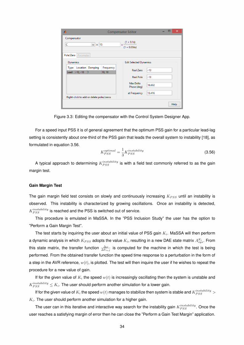
Figure 3.3: Editing the compensator with the Control System Designer App.
For a speed input PSS it is of general agreement that the optimum PSS gain for a particular lead-lag
setting is consistently about one-third of the PSS gain that leads the overall system to instability [18], as
formulated in equation 3.56.
KoptimalPSS =
1
3KinstabilityPSS (3.56)
A typical approach to determining KinstabilityPSS is with a field test commonly referred to as the gain
margin test.
Gain Margin Test
The gain margin field test consists on slowly and continuously increasing KPSS until an instability is
observed. This instability is characterized by growing oscillations. Once an instability is detected,
KinstabilityPSS is reached and the PSS is switched out of service.
This procedure is emulated in MaSSA. In the ”PSS Inclusion Study” the user has the option to
”Perform a Gain Margin Test”.
The test starts by inquiring the user about an initial value of PSS gain Ki. MaSSA will then perform
a dynamic analysis in which KPSS adopts the value Ki, resulting in a new DAE state matrix AKisys. From
this state matrix, the transfer function ∆ω∆Vref
is computed for the machine in which the test is being
performed. From the obtained transfer function the speed time response to a perturbation in the form of
a step in the AVR reference, w(t), is plotted. The test will then inquire the user if he wishes to repeat the
procedure for a new value of gain.
If for the given value of Ki the speed w(t) is increasingly oscillating then the system is unstable and
KinstabilityPSS ≤ Ki. The user should perform another simulation for a lower gain.
If for the given value ofKi the speedw(t) manages to stabilize then system is stable andKinstabilityPSS >
Ki. The user should perform another simulation for a higher gain.
The user can in this iterative and interactive way search for the instability gain KinstabilityPSS . Once the
user reaches a satisfying margin of error then he can close the ”Perform a Gain Test Margin” application.
34

3.4 PSS Inclusion Study
The flowchart in Figure 3.4 provides an overview of the developed ”PSS Inclusion Study”.
Figure 3.4: Flowchart of PSS Inclusion Study.
For a certain PSS, ”PSS Inclusion Study” performs a dynamic analysis of the system without PSS
and then it performs a dynamic analysis for each possible PSS location in the network. Then, power
transfer improvement, OPLI and the transfer functions are computed for the machines selected by the
user. The outputted results may consist on Bode plots, Root-loci, eigenvalues, OPLI, power transfer
improvements and it can also be a gain margin test.
35

3.5 Contributed Torques
The stabilizing torque contributed by the PSS, obtained in equation 3.52 can be viewed as in equation
3.57, partitioned in a component in phase with angle deviations and a component in phase with speed
deviations.
∆T stabe = T stabS ∆δ + T stabD ∆ω (3.57)
For a given oscillation, represented in frequency domain as s = σ + jω, the synchronizing and
damping coefficients of the stabilizing torque can be obtained as shown in equation 3.58. This is an
analogous operation as the one described in section 2.2.2.
T stabS = −Imag[∆T stab
e
∆ω ]σ2+ω2
ω
T stabD = Real[∆T stab
e
∆ω ]− T stabSσ
σ2+ω2
(3.58)
When plotting ∆T stabe in the ∆δ−∆ω plane, ideally it should lay in the ∆ω axis, meaning that it would
only contribute with damping torque without affecting the synchronizing torque of the system. When
there is some phase-lag, ∆T stabe should be in the first quadrant and close to the ∆ω axis, contributing
with both damping and synchronizing.
36

Chapter 4
Validation: 3-Machine 9-Bus Network
The popular Western System Coordinating Council (WSCC) 3-machine 9-bus network was chosen to
test the presented methodology.
In this network the generators are modelled as flux-decay machines regulated by fast, high gain
static AVR. The flux-decay machine is a 3rd-order system, the static AVR is a 1st-order system and the
network has three generators, making the total system a 12th-order model.
The system data and the power-flow for the nominal operation conditions are in Appendix B.
The flux-decay machine model was not yet implemented in MaSSA and it was complemented with
this generator model named GENDEC. The equations that define GENDEC are detailed in Appendix
C and its implementation was successfully validated through the use of a software package for power
system computation, analysis, and control named Power System Toolbox (PST).
MaSSA starts by reading the data files and then a window as illustrated in Figure 4.1 is prompt. The
user must choose what type of analysis wishes to perform.
Figure 4.1: MaSSA’s new ”Analysis” window.
When selecting ”PSS Inclusion Study”, the user is required to insert the PSS parameters, as depicted
in Figure 4.2 and then MaSSA proceeds to perform a dynamic analysis of the network without the PSS
and a dynamic analysis of the network with the chosen PSS.
In fact, MaSSA will do a dynamic analysis for each possible location for the PSS. So, in this particular
case, it will perform four dynamic analysis: one for the network without the PSS, another for the network
37

Figure 4.2: Insertig the parameters of the PSS under analysis.
with the PSS installed at machine of bus 1, another for the network with the PSS installed at machine of
bus 2 and another for the network with the PSS installed at machine of bus 3.
As mentioned before, a dynamic analysis with MaSSA consists on inducing a perturbation in the form
of increasing active power of the load at an arbitrary load bus. The system becomes unstable when an
eigenvalue of the system matrix crosses to the RHCP. In a window as shown in Figure 4.3 the user must
choose which load buses to increment. Load bus 5 was selected.
Figure 4.3: Choosing which load buses to increment when performing a dynamic analysis.
Also the type of load (”0” for constant power load, ”1” for constant current load and ”2” for constant
impedance load) and the operating point (i.e. the active power and reactive power at the chosen load
bus) must be defined by the user, as pictured in Figure 4.4. For the present case all loads are considered
to be modelled as constant power and the operating point is the nominal case, with PL5= 1.25 pu and
QL5= 0.5 pu.
Once all the presented specifications are defined the four dynamic analyses are computed.
38

Figure 4.4: Inserting the type of load and operating point.
A ”PSS Inclusion Study Results” window shown in Figure 4.5 appears and from it the user may
choose which results to print/plot.
Figure 4.5: Choosing which results to print or plot.
In the ”Options” panel the user selects for which machines the results should be presented, up to six
machines. The user may compare results from before the PSS inclusion with after PSS inclusion and it
can also compare results between the PSS installed at different machines.
4.1 Analysis Before PSS Inclusion
A dynamic analysis of the system is performed and the resulting eigenvalues, as well as respective
frequencies and damping ratios1, for the nominal case are presented in Table 4.1. It is clear from it that
1Damping ratio: ξ = − σ√σ2+ω2
39

the oscillations of concern for stability are the ones corresponding to the oscillating mode λ1,2, which is
in the RHCP, and the oscillating mode λ4,5, which is close to the RHCP.
Mode Eigenvalue Frequency [Hz] Damping
λ1,2 0.1718± j9.0447 1.440 −0.019
λ3 0 - -λ4,5 −0.0460± j13.2499 2.109 0.003
λ6,7 −0.1975 - -λ7,8 −2.7568± j7.9476 1.265 0.328
λ9,10 −2.7696± j11.8356 1.884 0.228
λ11,12 −2.8396± j8.2657 1.316 0.325
Table 4.1: Eigenvalues before PSS inclusion for the nominal case.
Because there is already a mode in the RHCP at the nominal case, the system is unstable even
before a perturbation is induced.
The zero eigenvalue appears because of redundancy in angle (the machine’s speeds and angles
are represented in absolute terms therefore introducing redundancies in the state variables) and so the
resulting state matrix is singular.
Tables 4.2 and 4.3 show the system’s state variables associated with the oscillations of concern λ1,2
and λ4,5. In both cases, rotor angle and rotor speed deviations are the states that contribute the most
for the modes and so the oscillations are of electromechanical nature. The state variables vector ∆x as
well as the control variables vector ∆u are as described by equations 4.1 and 4.2.
∆x =[
∆δ1 ∆ω1 ∆E′q1 ∆Efd1 ∆δ2 ∆ω2 ∆E′q2 ∆Efd2 ∆δ3 ∆ω3 ∆E′q3 ∆Efd3
]T(4.1)
∆u =[
∆TM1 ∆Vref1 ∆TM2 ∆Vref2 ∆TM3 ∆Vref3
]T(4.2)
Noticing the frequency of these electromechanical oscillations hints that they are most likely local modes
of oscillation, resulting from a single machine swinging relative to the rest of the system.
Machine 1 Machine 2 Machine 3
States ∆δ1 ∆ω1 ∆δ2 ∆ω2 ∆E′q2 ∆Efd2 ∆δ3 ∆ω3
Participation 0.41 0.41 1.00 1.00 0.11 0.11 0.14 0.14
Table 4.2: Participation factors of the states associated with mode λ1,2.
Machine 2 Machine 3
States ∆δ2 ∆ω2 ∆δ3 ∆ω3
Participation 0.20 0.20 1.00 1.00
Table 4.3: Participation factors of the states associated with mode λ4,5.
Thus, this system is an adequate candidate for PSS installation because its stability margins are
40

Figure 4.6: Time responses of δ and ω for a step in Vref2, with no PSS included in the network.
significantly reduced due to the presence of undamped electromechanical oscillations that limit the sys-
tem’s power transfer.
Figure 4.6 shows, for each machine, the time responses of the rotor’s angle and velocity when a step
signal is imposed in the AVR reference of machine 2, i.e when the system is subjected to a disturbance.
The system becomes unstable and this instability occurs in the form of increasing angular swings,
leading to loss of synchronism and a progressive increase in angular separation between rotors. The
rotors are continuously accelerated-decelerated and oscillate with an increasing amplitude: these are
the electromechanical oscillations.
The time response of Figure 4.6 is coherent with the frequency analysis of Table 4.1 that shows an
eigenalue in the RHCP.
Imposing a step disturbance in either Vref1 or Vref3 yields analogous results.
4.2 Analysis After PSS Inclusion
A dynamic analysis of the system is performed for each possible scenario of the PSS location, that is,
for the PSS included at each machine.
A single-stage with washout filter PSS as represented in Figure 4.7 was chosen and its parameters
are as shown in Table 4.4.
Figure 4.7: Chosen PSS structure.
41

KPSS TW [sec] T1 [sec] T2 [sec]
10 10 0.5 0.01
Table 4.4: Chosen PSS parameters.
The resulting eigenvalues for each dynamic analysis are presented in Tables 4.5, 4.6 and 4.7 for the
nominal case, i.e with PL5= 1.25 pu and QL5
= 0.5 pu.
The inclusion of the PSS in the system will bring two more eigenvalues, that is to say two more state
variables: ∆xp1 contributed by the washout filter and ∆Vs contributed by the lead-lag block of the phase
compensation stage.
Mode Eigenvalue Frequency [Hz] Damping
λ1,2 0.2104± j9.8667 1.570 −0.021
λ3 0 - -λ4,5 −0.0448± j13.2702 2.112 0.003
λ6 −0.1022 - -λ7 −0.1934 - -λ8,9 −2.0458± j7.6108 1.211 0.260
λ10,11 −2.8719± j8.0831 1.286 0.335
λ12,13 −3.4864± j11.5768 1.843 0.288
λ14 −100.05 - -
Table 4.5: Eigenvalues after PSS inclusion in machine 1 for the nominal case.
Mode Eigenvalue Frequency [Hz] Damping
λ1 0 - -λ2 −0.1109 - -λ3 −0.1790 - -λ4,5 −0.8785± j12.6080 2.007 0.070
λ6,7 −0.9392± j15.8188 2.518 0.059
λ8,9 −1.3992± j6.3476 1.010 0.215
λ10,11 −1.8944± j9.6291 1.533 0.193
λ12,13 −2.7206± j7.8698 1.253 0.327
λ14 −100.84 - -
Table 4.6: Eigenvalues after PSS inclusion in machine 2 for the nominal case.
In short and comparing to the system without PSS:
• including the PSS at machine 1 worsens the system’s stability;
• including the PSS at machine 2 improves the system’s stability the most;
• including the PSS at machine 3 improves the system’s stability.
The above statements are reinforced with the analysis of Figures 4.8, 4.9 and 4.10, which show the
time responses of the angles and velocities of the rotors when a step signal is imposed in the AVR
reference of the machine in which the PSS is installed.
42

Mode Eigenvalue Frequency [Hz] Damping
λ1 0 - -λ2 −0.1058 - -λ3,4 −0.1603± j9.0136 1.435 0.018
λ5 −0.1873 - -λ6,7 −0.5729± j17.0633 2.716 0.034
λ8,9 −1.9160± j6.3473 1.010 0.289
λ10,11 −2.3614± j11.7837 1.875 0.196
λ12,13 −2.7515± j8.2287 1.310 0.317
λ14 −10096 - -
Table 4.7: Eigenvalues after PSS inclusion in machine 3 for the nominal case.
Figure 4.8: Time responses of δ and ω for a step in Vref1, with PSS included in machine 1.
Subjecting the system to a disturbance when the PSS is installed at machine 1 leads the system to
rotor angle instability in similarity with what happened before PSS inclusion. This is coherent with Table
4.5 that shows an eigenvalue in the RHCP.
Subjecting the system to a disturbance when the PSS is installed at machine 2 yields very satisfying
results: the rotors velocities start with a transient instability, swinging relative to each other, but in about
four seconds they align and converge to the same limit - the synchronous velocity limit - with barely no
oscillation.
Because the disturbance is inflicted on machine 2, the rotor angle of machine 2 is the one that
initially suffers the biggest excursion but, at around two seconds after the disturbance, all three angles
start increasing at the same pace, meaning that all three velocities are synchronized.
Subjecting the system to a disturbance when the PSS is installed at machine 3 also yields satisfying
results: the rotors velocities swing relative to each other with decreasing amplitude and in around twelve
seconds they are synchronized. Although effective, it still takes circa three times longer to damp the
oscillations when comparing to the performance of the PSS installed at machine 2.
43

Figure 4.9: Time responses of δ and ω for a step in Vref2, with PSS included in machine 2.
Figure 4.10: Time responses of δ and ω for a step in Vref3, with PSS included in machine 3.
4.3 PSS Location
Given the PSS parameters of Table 4.4, the optimal machine in which to install the PSS is determined
by the power transfer capability criterion and then confirmed by the OPLI technique.
Power Transfer Capability
Before PSS inclusion the system was unstable at the nominal operation, with PL5 = 1.25 pu. The com-
pensated system should improve the power transfer capability of the network and the optimal location
for the PSS corresponds to the machine at which the power transfer improves the most.
Table 4.8 shows, for each possible PSS location, the active power at the load bus 5 at which an
44

unstable mode is detected.
Machine 1 Machine 2 Machine 3
P instabilityL5 1.25 pu 4.92 pu 2.49 pu
Table 4.8: Active power at load bus 5 at which the system becomes unstable.
Table 4.9 expresses both in pu and % the improvement in power transfer capability, compared to the
system without PSS.
Machine 1 Machine 2 Machine 3
Power Transfer Improvement [pu] 0 3.67 pu 1.24 pu
Power Transfer Improvement [%] 0 293.6 % 99.2 %
Table 4.9: Improvement of the system’s power transfer capability by PSS inclusion.
Because including the PSS at machine 2 improves the system’s power transfer capability the most,
this is the optimal machine for the PSS.
Upon the user’s request, ”PSS Inclusion Study” computes the above results and concludes on the
optimal machine.
OPLI
From Tables 4.2 and 4.3 the swing-loop participation ratio ρ introduced in section 3.2.2 can be calculated
as in equations 4.3 and 4.4 for the modes λ1,2 and λ4,5 before PSS inclusion. The remainder modes do
not satisfy ρ > 0.5 and so they are not considered electromechanical modes.
ρ1,2 =0.41 + 0.41 + 1.00 + 1.00 + 0.11 + 0.11 + 0.14 + 0.14
0.41 + 0.41 + 1.00 + 1.00 + 0.14 + 0.14≈ 0.93 (4.3)
ρ4,5 =0.20 + 0.20 + 1.00 + 1.00
0.20 + 0.20 + 1.00 + 1.00= 1 (4.4)
The mode λ4,5 has the highest swing-loop participation ratio ρ and so, according to the OPLI tech-
nique, this will be the critical swing mode before PSS inclusion λ0. This is debatable because λ1,2 is well
into the RHCP and λ4,5 is not.
Including a PSS will not make new electromechanical modes appear nor will it make the existing
ones disappear, it will only damp them. So, in some simpler cases, it is possible to identify these modes
before and after PSS inclusion.
Tables 4.10 to 4.15 show the states associated with the two modes that have the highest swing-loop
participation ratio ρ, after PSS inclusion. Each set of two modes after PSS inclusion should correlate to
the modes λ1,2 and λ4,5 before the inclusion of the PSS.
Comparing Tables 4.10 and 4.11 to Tables 4.2 and 4.3 it is immediate to conclude that modes λ1,2
and λ4,5 before PSS inclusion correspond respectively to modes λM11,2 and λM1
4,5 after PSS inclusion in
machine 1.
45

Machine 1 Machine 2 Machine 3
States ∆δ1 ∆ω1 ∆E′q1 ∆Efd1 ∆δ2 ∆ω2 ∆E′q2 ∆Efd2 ∆E′q3 ∆Efd3
Participation 0.37 0.37 0.46 0.40 1.00 1.00 0.35 0.32 0.16 0.15
Table 4.10: Participation factors of the states associated with mode λM11,2 for PSS installed at machine 1.
Machine 2 Machine 3
States ∆δ2 ∆ω2 ∆δ3 ∆ω3
Participation 0.20 0.20 1.00 1.00
Table 4.11: Participation factors of the states associated with mode λM14,5 for PSS installed at machine 1.
The swing-loop participation ratios for the electromechanical modes when including the PSS at ma-
chine 1 are ρM11,2 ≈ 0.60 and ρM1
4,5 = 1 and so it is safe to say that the critical swing mode λ′ = λM14,5
corresponds to λ0 = λ4,5 .
Machine 2 Machine 3
States ∆δ2 ∆ω2 ∆E′q2 ∆Efd2 ∆δ3 ∆ω3 ∆E′q3 ∆Efd3
Participation 0.13 0.13 0.28 0.26 1.00 1.00 0.30 0.29
Table 4.12: Participation factors of the states associated with mode λM24,5 for PSS installed at machine 2.
Machine 1 Machine 2
States ∆δ1 ∆ω1 ∆E′q1 ∆δ2 ∆ω2 ∆E′q2 ∆Efd2 ∆y
Participation 0.24 0.24 0.11 1.00 0.99 0.64 0.55 0.23
Table 4.13: Participation factors of the states associated with mode λM28,9 for PSS installed at machine 2.
Comparing Tables 4.12 and 4.13 to Tables 4.2 and 4.3, in particular noticing the participation factors
of states ∆δ and ∆ω, there is some confidence in stating that modes λ1,2 and λ4,5 before PSS inclusion
probably correspond to modes λM28,9 and λM2
4,5 after PSS inclusion in machine 2, respectively.
The swing-loop participation ratios for the electromechanical modes when including the PSS at ma-
chine 2 are ρM24,5 ≈ 0.67 and ρM2
8,9 ≈ 0.62 and so it is safe to say that the critical swing mode λ′ = λM28,9
corresponds to λ0 = λ4,5 .
Machine 1 Machine 2 Machine 3
States ∆δ1 ∆ω1 ∆δ2 ∆ω2 ∆E′q2 ∆Efd2 ∆δ3 ∆ω3
Participation 0.38 0.38 1.00 1.00 0.13 0.12 0.12 0.12
Table 4.14: Participation factors of the states associated with mode λM33,4 for PSS installed at machine 3.
Comparing Tables 4.14 and 4.15 to Tables 4.2 and 4.3, in particular noticing the participation factors
of states ∆δ and ∆ω, there is some confidence in stating that modes λ1,2 and λ4,5 before PSS inclusion
46

Machine 3
States ∆δ3 ∆ω3 ∆E′q3 ∆Efd3 ∆Vs
Participation 0.89 0.89 1.00 0.97 0.12
Table 4.15: Participation factors of the states associated with mode λM36,7 for PSS installed at machine 3.
probably correspond to modes λM33,4 and λM3
6,7 after PSS inclusion in machine 3, respectively.
The swing-loop participation ratios for the electromechanical modes when including the PSS at ma-
chine 3 are ρM33,4 ≈ 0.92 and ρM3
6,7 ≈ 0.46 and so the critical swing mode is λ′ = λM33,4 .
With machine 3 the OPLI technique presents two problems: firstly, λM36,7 is not even considered an
electromechanical mode because it does not satisfy ρ > 0.5; secondly, it considers λM33,4 to be the critical
swing mode when λM33,4 most likely does not correspond to λ0 = λ4,5. This means that OPLI will be
measuring the difference in the AVR’s transfer function for two eigenvalues that do not correlate with
each other, which is conceptually meaningless.
Nevertheless, the OPLI technique still corroborates that the optimal site for PSS inclusion is at ma-
chine 2, that the second optimal site is at machine 3 and that the worst is at machine 1, as can be seen
from Table 4.16.
Machine 1 Machine 2 Machine 3
OPLI 0.0013 1.9037 0.5583
Table 4.16: OPLI computed for each machine.
4.4 PSS Tuning
The parameters shown in Table 4.4 correspond to the optimal PSS tuning when it is installed at machine
2, the optimal site for PSS inclusion. These parameters satisfy the tuning criteria stipulated for the
washout filter, the phase compensation and the gain.
Washout Filter
Typical values for the washout filter time constant TW (when preceded by KPSS) are in the range of 10
seconds. Assuming this value for TW , the washout filter transfer function is as presented in equation 4.5
and behaves as shown in Table 4.17.
In steady-state operation GW (s) is null, not allowing the PSS to interfere with the normal, stable op-
eration of the power system. When the oscillations of concern arise, it becomes nearly unitary, activating
the PSS. In the present case, such oscillations of concern correspond to the modes λ1,2 and λ4,5 of the
system before PSS inclusion.
GW (s) =s10
1 + s10(4.5)
47

Steady State λ1,2 λ4,5
GW (λ) 0 0.999796∠0.633521◦ 0.999998∠0.432422◦
Table 4.17: Washout filter behaviour for steady-state condition and for the oscillations of concern.
Because it has a nearly unitary magnitude and almost null phase, the washout filter will have virtually
no relevance in the phase compensation tuning stage.
Phase Compensation
Figure 4.11 shows the Bode diagrams of three systems:
• the GEP system for machine 2 in red, defined by ∆Telower2
∆Vref,2(s);
• the PSS system in green, defined by ∆Vs
∆ν2(s);
• the system resulting from the series of the two above in blue, defined by ∆T stabe
∆ν2(s)
Figure 4.11: Bode diagram of GGEP (s), GPSS(s) and GGEP (s)GPSS(s).
The torque contributed solely by action of the PSS, ∆T stabe , should be in phase with speed deviations
∆ω. To achieve this, the phase characteristic of ∆T stabe
∆ν2(s) should be as close to zero as possible in the
frequency range of concern, that is, in the frequency range of the local modes of oscillation. Since
this is a short range to analyse, the frequency axis is represented in linear scale rather than the typical
logarithmic scale.
Looking at the blue Bode, indeed the chosen T1 and T2 PSS values manage to keep the phase close
to zero (more precisely, not exceeding ±20◦ from zero) from around ω = 9.4 rad/sec to ω = 12.2 rad/sec.
Figure 4.12 shows the Control System Designer launched for this particular case. From the Compen-
sator Editor dialog box the user can see that the chosen PSS parameters T1 = 0.5 sec and T2 = 0.01 sec
48

Figure 4.12: Using the Control System Designer to tune the 9-bus 3-machine PSS.
correspond to a zero in ω = −2 rad/sec and a pole in ω = −100 rad/sec and that they will introduce a
maximum phase of φm = 73.901◦ at frequency ωm = 14.142 rad/sec.
At this point, although there is already a significant compensation of the phase lag, the user may try
to further improve the compensation by introducing a new lead-lag block characterized by T3 and T4.
Observing the compensated blue Bode, a second lead-lag block would be worth implementing if it would
manage to: either significantly compensate for the abrupt 90◦ phase lag at around ω = 9 rad/sec; or
to significantly compensate for the abrupt 90◦ phase lead at around ω = 13 rad/sec, without damaging
the already satisfying phase that exists between. As mentioned before, too much phase lead is also
detrimental to the system performance since it worsens synchronizing torque.
The fact is that introducing (or removing) so much phase in such a short range of frequencies is
not implementable, it would necessarily deteriorate the range in which the phase manages to be close
to zero. The bigger the amount of phase introduced by the compensator, the wider the frequency
range in which it acts. Implementing a second lead-lag is not beneficial in this particular case. It is
usually advantageous when compensating systems with a IEEET1 AVR model, since this type of AVR
introduces a phase of −180◦ whilst the ST AVR model used in the present case introduces just −90◦.
Gain Margin Test
For KPSS = 10 it is already known from Figure 4.9 that the system is stable. Thus, a value of KPSS = 50
is chosen to start the gain margin test. Figure 4.13 shows that the system is unstable for this gain and
so the simulation is repeated for KPSS = 30, the average between the stable and unstable gains.
For KPSS = 30 the system is stable but with a longer settling time when compared with the results
for KPSS = 10, hinting that the optimal gain should be closer to KPSS = 10 than to KPSS = 30.
Again the average value between stable and unstable gains is considered and Figure 4.15 shows that
the system is stable for KPSS = 40. It takes around 100 seconds for the speed to reach synchronism,
49

Figure 4.13: Gain margin test for KPSS = 50.
Figure 4.14: Gain margin test for KPSS = 30.
circa twenty times more when compared to KPSS = 10, hinting that the instability gain should be close
to KPSS = 40.
For KPSS = 41 the system becomes unstable, as seen in Figure 4.16. Because it is closer to the
KinstabilityPSS limit, this instability has a much slower increase of the speed swings when compared to the
KPSS = 50 instability.
Considering KPSS = 41 close enough to the KinstabilityPSS limit, the optimal gain is thus calculated as
in equation 4.6.
KoptimalPSS =
1
341 ≈ 13.67 (4.6)
This means that adopting a value for KPSS closer to 13.6 should yield a better PSS performance than
50

Figure 4.15: Gain margin test for KPSS = 40.
Figure 4.16: Gain margin test for KPSS = 41.
the considered KPSS = 10. In fact, adopting KPSS = 13 does allow a higher power transfer capability,
as shown in Table 4.18, which should be compared with Table 4.9.
Machine 1 Machine 2 Machine 3
Power Transfer Improvement [pu] 0 3.68 pu 1.34 pu
Table 4.18: Improvement of the system’s power transfer capability by PSS inclusion with KPSS = 13.
Because it is such a negligible improvement (0.01 pu for machine 2 and 0.1 pu for machine 3) the
originally adopted KPSS = 10 is considered to be equally satisfying.
51

52

Chapter 5
Results
Two systems whose stabilities are improved by PSS inclusion are presented: the two-area system and
the 10-machine 39-bus system.
The two-area system is chosen to illustrate the detrimental impact that inter-area oscillations have
on power systems and how the PSS helps to mitigate this problem. The impact that the connecting
transmission lines as well as the amount of power transfer have on the system’s stability is analyzed. It
is also shown that the load elasticity influences the stability limit.
The 10-machine 39-bus network is used to test the effect of the AVR on stability. In particular, it is
shown how the chosen AVR model, either ST or IEEET1, as well as the AVR gain KA influence the
system’s response to a small perturbation. Following, the impact of installing one PSS in this network,
and then of installing multiple PSS’s is discussed.
5.1 Two-Area System
The growing trend of interconnecting generating areas is critical in ensuring the reliability of the power
system and often presents itself as an economically attractive solution.
Conflictingly, interconnected power systems are precisely one of the main contributors for oscillatory
instability. As a consequence of growth in interconnections is the formation of closely coupled machines
linked by weak lines. With heavy power transfers between areas, such systems exhibit inter-area modes
of oscillation.
Figure 5.1 represents a four-generator ten-bus two-area power system. The areas, consisting of two
coupled generating units, are linked by three tie lines. The total connected load is 2734 MW and the
system is operating with area 1 exporting 153.28 MW to area 2.
The system data as well as the power-flow for the nominal operation conditions are presented in
Appendix D.
The generating units consist on a fourth-order round rotor synchronous machine with no saturation
model, referred to as GENRED in MaSSA, and a first-order static exciter model, referred to as ST. The
overall system will then be characterized by twenty eigenvalues. The machines have null damping and
53

Figure 5.1: Two-area system, adapted from [21].
the exciter is a high-gain fast-acting one. Both loads are considered to be modelled as constant power.
To perform a dynamic analysis of the system the active power at load bus 10 is incremented and
the system becomes unstable at P instabilityL10= 16.26 pu. It is worth mentioning that increasing the
perturbation until PL10 = 25.00 pu does not induce the power-flow to diverge, underlining how important
it is to have a dynamic analysis complementing the static analysis.
The eigenvalues for the nominal case, with PL10= 15.75 pu, are presented in Table 5.1.
Mode Eigenvalue Frequency [Hz] Damping
λ1 0 - -λ2 0 - -λ3,4 −0.0162± j4.6075 0.7333 +0.004
λ5,6 −0.7765± j7.4899 1.1920 +0.103
λ7,8 −0.7848± j6.8119 1.0841 +0.114
λ9 −4.3111 - -λ10,11 −4.4273± j17.3543 2.7620 +0.247
λ12,13 −4.5311± j0.0856 0.0136 +1.000
λ14 −4.6827 - -λ15,16 −5.0989± j11.6640 1.8564 +0.401
λ17,18 −5.2733± j7.3091 1.1633 +0.585
λ19,20 −5.3341± j6.9898 1.1125 +0.607
Table 5.1: Eigenvalues before PSS inclusion for the nominal case.
The oscillation of concern is the least damped oscillating mode λ3,4 = −0.0162 ± j4.6075, which is
fairly close to the RHCP and has a rather insufficient damping ratio of ξ = 0.004.
The frequency of λ3,4 suggests that it is an inter-area oscillating mode, which is expectable since it
is a two-area system. Table 5.2 shows that this mode is solely associated with mechanical states and
so it should be responsive to the action of a PSS.
A ”PSS Inclusion Study” analysis for the same perturbation at load bus 10 is performed considering
a two-stage PSS with washout as pictured in Figure 2.7. Its parameters are presented in Table 5.3.
54

Machine 1 Machine 2 Machine 3 Machine 4
States ∆δ1 ∆ω1 ∆δ2 ∆ω2 ∆δ3 ∆ω3 ∆δ4 ∆ω4
Participation 1.00 1.00 0.81 0.81 0.64 0.64 0.54 0.54
Table 5.2: Participation factors of the states associated with mode λ3,4.
KPSS TW [sec] T1 [sec] T2 [sec] T3 [sec] T4 [sec]
25 10 0.047 0.021 3.0 5.4
Table 5.3: Chosen PSS parameters.
Table 5.4 shows, for each possible PSS location, the active power at load bus 10 at which an unstable
mode is detected. For any case, instability is delayed from the original situation P instabilityL10= 16.26 pu.
Machine 1 Machine 2 Machine 3 Machine 4
P instabilityL1019.78 pu 19.21 pu 23.30 pu 18.19 pu
Table 5.4: Active power at load bus 10 at which the system becomes unstable, for each possible PSSlocation.
Table 5.5 expresses both in pu and % the improvement of the system’s power transfer capability for
each possible PSS location. It is immediate to see that machine 3 is the optimal machine to install the
PSS.
Machine 1 Machine 2 Machine 3 Machine 4
Power Transfer Improvement [pu] 3.52 pu 2.95 pu 7.04 pu 1.93 pu
Power Transfer Improvement [%] 21.65 % 18.14 % 43.29 % 11.87 %
Table 5.5: Improvement of the system’s power transfer capability by PSS inclusion.
The eigenvalues of the system with the PSS installed at machine 3 are presented in Table 5.6 for the
nominal case, with PL10 = 15.75 pu.
The original oscillation of concern λ3,4 corresponds now to the significantly more damped oscillating
mode λ5,6 = −0.1986 ± j4.6711 with a damping ratio of ξ = 0.042, which is circa ten times higher than
the original damping ratio ξ = 0.004.
Load Elasticity Effect
The load elasticity determines the load power dependence in relation to the bus voltage [22] and influ-
ences the system’s stability. Equation 5.1 and equation 5.2 express how the active power load PL and
reactive power load QL relate to the bus voltage V by their respective elasticities np and nq.
PL = PL0
(V
V0
)np
(5.1)
55

Mode Eigenvalue Frequency [Hz] Damping
λ1 0 - -λ2 0 - -λ3 −0.0753 - -λ4 −0.1956 - -λ5,6 −0.1986± j4.6711 0.7434 +0.042
λ7,8 −0.7988± j6.8218 1.0857 +0.116
λ9,10 −0.9274± j9.2481 1.4719 +0.100
λ11 −3.9518 - -λ12 −4.3550 - -λ13,14 −4.3945± j17.3556 2.7622 +0.245
λ15 −4.5734 - -λ16 −4.6631 - -λ17,18 −4.8237± j11.5626 1.8402 +0.385
λ19,20 −5.2456± j7.2115 1.1477 +0.588
λ21,22 −5.4845± j5.3438 0.8505 +0.716
λ23 −47.7219 - -
Table 5.6: Eigenvalues after PSS inclusion in machine 3 for the nominal case.
QL = QL0
(V
V0
)nq
(5.2)
Deriving with respect to the bus voltage V , the partial derivatives in equation 5.3 and equation 5.4
are obtained.∂PL∂V
=PL0
Vnp
0
npVnp−1 (5.3)
∂QL∂V
=QL0
Vnq
0
nqVnq−1 (5.4)
For null elasticity the load is referred to as constant power load. When the elasticity is unitary the
load is referred to as constant current load and when the elasticity is 2 the load is referred to as constant
impedance load. Table 5.7 shows the resulting active power partial derivatives for each type of load
elasticity.
Constant Power Constant Current Constant Impedance
∂PL
∂V = 0 ∂PL
∂V =PL0
V0
∂PL
∂V = 2PL0
V 20V
Table 5.7: Partial derivatives contributed by each type of load model.
The contribution of load elasticities to the system’s stability is taken into account in equation 3.6 of
the DAE model presented in section 3.1, i.e is taken into account in the network equation of the load
buses. More precisely, the linearized partial derivatives of Table 5.7 are summed in matrix D7 of this
DAE equation because D7 is the matrix associated with the state variable vector Vl that represents the
voltages of the load buses. In doing so, it will affect the resulting system matrix Asys and consequently
it will as well affect the eigenvalues of the system.
Table 5.8 shows, for each possible PSS location, how P instabilityL10changes with the type of load.
56

Constant Power Constant Current Constant Impedance
No PSS 16.26 pu 16.27 pu 16.30 pu
PSS at Machine 1 19.78 pu 21.65 pu 24.45 pu
PSS at Machine 2 19.21 pu 21.44 pu 20.75 pu
PSS at Machine 3 23.30 pu 24.25 pu 23.36 pu
PSS at Machine 4 18.19 pu 19.86 pu 22.51 pu
Table 5.8: Active power at load bus 10 at which the system becomes unstable for different load elastici-ties.
Constant power is consistently the least favourable scenario. However, it is not possible to assert
which delays instability the most, if constant current or constant impedance.
Tie Line Effect
As mentioned before, weakly connected power systems are particularly prone to inter-area oscillations.
Hence, the number of tie lines connecting the two areas influences the system’s stability.
The higher the number of tie lines the stronger is the link between areas and so the closer they
are, electrically speaking. This makes the system more robust to instability, as corroborated by Table
5.9, showing the oscillating modes of concern moving towards the RHCP as the number of tie lines
decreases. With one tie line only, the system is unstable at nominal operation.
3 Lines 2 Lines 1 Line
Mode Eigenvalue Mode Eigenvalue Mode Eigenvalue
λ1 0 λ1 0 λ1,2 +0.0012± j3.0634
λ2 0 λ2 0 λ3 0
λ3,4 −0.0162± j4.6075 λ3,4 −0.0139± j4.0901 λ4 0
λ5,6 −0.7765± j7.4899 λ5,6 −0.7736± j6.7828 λ5,6 −0.7448± j6.7496
λ7,8 −0.7848± j6.8119 λ7,8 −0.7796± j7.4526 λ7,8 −0.7749± j7.4035
λ9 −4.3111 λ9 −4.3083 λ9 −4.3002
λ10,11 −4.4273± j17.3543 λ10,11 −4.4511± j17.3895 λ10,11 −4.4815± j17.5542
λ12,13 −4.5311± j0.0856 λ12,13 −4.5294± j0.0818 λ12,13 −4.5220± j0.0646
λ14 −4.6827 λ14 −4.7034 λ14 −4.7397
λ15,16 −5.0989± j11.6640 λ15,16 −4.9900± j12.5214 λ15,16 −4.8296± j14.0524
λ17,18 −5.2733± j7.3091 λ17,18 −5.2683± j7.3624 λ17,18 −5.2658± j7.4548
λ19,20 −5.3341± j6.9898 λ19,20 −5.3162± j7.1283 λ19,20 −5.3064± j7.3006
Table 5.9: Eigenvalues for different tie lines scenarios before PSS inclusion for the nominal case.
Table 5.10 shows that with the loss of one line or even with the loss of two lines and with the PSS
installed at machine 3, the system is still stable at the nominal operation.
The PSS is thus a major contribution to extending the system’s stability limits and Table 5.11 proves
this, showing how P instabilityL10changes with the number of tie lines, with and without the PSS.
57

3 Lines 2 Lines 1 Line
Mode Eigenvalue Mode Eigenvalue Mode Eigenvalue
λ1 0 λ1 0 λ1 0
λ2 0 λ2 0 λ2 0
λ3 −0.0753 λ3 −0.0748 λ3 −0.0734
λ4 −0.1956 λ4,5 −0.1559± j4.1258 λ4,5 −0.0819± j3.0755
λ5,6 −0.1986± j4.6711 λ6 −0.1959 λ6 −0.1967
λ7,8 −0.7988± j6.8218 λ7,8 −0.7804± j6.7857 λ7,8 −0.7462± j6.7497
λ9,10 −0.9274± j9.2481 λ9,10 −0.9276± j9.2322 λ9,10 −0.9384± j9.2156
λ11 −3.9518 λ11 −3.9743 λ11 −4.0153
λ12 −4.3550 λ12 −4.3578 λ12 −4.3703
λ13,14 −4.3945± j17.3556 λ13,14 −4.4202± j17.3908 λ13,14 −4.4596± j17.5553
λ15 −4.5734 λ15 −4.5350 λ15 −4.4670
λ16 −4.6631 λ16 −4.7005 λ16,17 −4.6735± j14.0430
λ17,18 −4.8237± j11.5626 λ17,18 −4.7686± j12.4730 λ18 −4.7448
λ19,20 −5.2456± j7.2115 λ19,20 −5.2485± j7.3129 λ19,20 −5.2590± j7.4440
λ21,22 −5.4845± j5.3438 λ21,22 −5.4508± j5.3944 λ21,22 −5.3983± j5.4822
λ23 −47.7219 λ23 −47.7179 λ23 −47.7108
Table 5.10: Eigenvalues for different tie lines scenarios with PSS installed at machine 3 for the nominalcase.
3 Lines 2 Lines 1 Line
No PSS 16.26 pu 16.35 pu 15.75 pu
PSS at Machine 3 23.30 pu 22.45 pu 19.55 pu
Table 5.11: Active power at load bus 10 at which the system becomes unstable for different tie linesscenarios.
Power Transfer Between Areas Effect
When the load demand of area 2 exceeds its generating capacity and area 1 has a surplus of generating
capacity, then the load demand is satisfied by area 1 exporting power to area 2 through the connecting
transmission lines. The amount of power transfer is thus determined by the power balance of the areas.
The power balance within each area is determined by equation 5.5. When P > 0 there is surplus of
generating capacity, when P < 0 there is deficit of generating capacity.
P = PG − PL (5.5)
Tables 5.12 to 5.16 show how different load demands in each area determine the amount of power
transfer. In any case, the total connected load remains 2734 MW.
The amount of exported power impacts the system’s stability since heavy power transfers between
areas contribute to the rise of inter-area oscillations.
Figure 5.2 expresses, for each power transfer scenario presented in Tables 5.12 to 5.16, the amount
of incremented power at load bus 10 that leads the system to instability. As expected, the lower the
58

Area 1 Area 2
PGA1= 1400 MW PLA1
= 1159 MW PGA2= 1421.72 MW PLA2
= 1575 MW
PA1 = 241 MW PA2 = −153.28 MW
Table 5.12: Area 1 transfers 153.28 MW to area 2.
Area 1 Area 2
PGA1= 1400 MW PLA1
= 1206.14 MW PGA2= 1421.72 MW PLA2
= 1527.86 MW
PA1 = 193.86 MW PA2 = −106.14 MW
Table 5.13: Area 1 transfers 106.14 MW to area 2.
Area 1 Area 2
PGA1= 1400 MW PLA1
= 1256.14 MW PGA2= 1421.72 MW PLA2
= 1477.86 MW
PA1 = 143.86 MW PA2 = −56.14 MW
Table 5.14: Area 1 transfers 56.14 MW to area 2.
Area 1 Area 2
PGA1= 1400 MW PLA1
= 1256.14 MW PGA2= 1306.72 MW PLA2
= 1427.86 MW
PA1 = 93.86 MW PA2 = −6.14 MW
Table 5.15: Area 1 transfers 6.14 MW to area 2.
Area 1 Area 2
PGA1= 1400 MW PLA1
= 1356.14 MW PGA2= 1421.72 MW PLA2
= 1377.86 MW
PA1 = 43.86 MW PA2 = 43.86 MW
Table 5.16: No power transfer between areas.
power transfer between areas, the more robust the system is. This effect becomes even more evident
with the loss of lines.
Installing a PSS at machine 3 significantly extends the system’s stability margins for any power
transfer scenario, as shown in Figure 5.3. Regardless of installing or not a PSS, the trend remains true:
the lower the power transfer the better the stability.
5.2 10-machine 39-bus System
The IEEE 10-machine 39-bus system, commonly known as the New England Power System, is pre-
sented in Figure E.1 in Appendix E, along with the system’s data and power-flow at the nominal operation
conditions [23].
Again, the generating units are modelled as GENRED machines with parameters defined in Table
E.1 of Appendix E. Machine 1 represents the aggregation of a large number of machines, hence its high
59
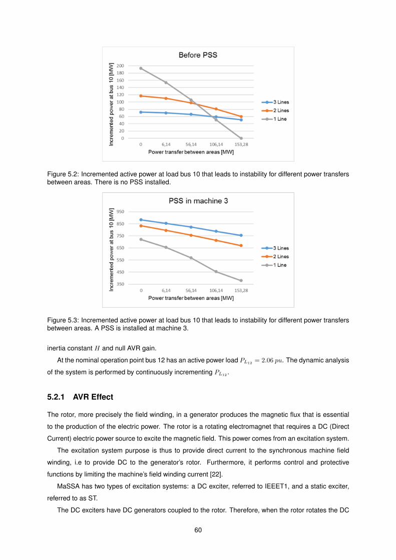
Figure 5.2: Incremented active power at load bus 10 that leads to instability for different power transfersbetween areas. There is no PSS installed.
Figure 5.3: Incremented active power at load bus 10 that leads to instability for different power transfersbetween areas. A PSS is installed at machine 3.
inertia constant H and null AVR gain.
At the nominal operation point bus 12 has an active power load PL12= 2.06 pu. The dynamic analysis
of the system is performed by continuously incrementing PL12.
5.2.1 AVR Effect
The rotor, more precisely the field winding, in a generator produces the magnetic flux that is essential
to the production of the electric power. The rotor is a rotating electromagnet that requires a DC (Direct
Current) electric power source to excite the magnetic field. This power comes from an excitation system.
The excitation system purpose is thus to provide direct current to the synchronous machine field
winding, i.e to provide DC to the generator’s rotor. Furthermore, it performs control and protective
functions by limiting the machine’s field winding current [22].
MaSSA has two types of excitation systems: a DC exciter, referred to IEEET1, and a static exciter,
referred to as ST.
The DC exciters have DC generators coupled to the rotor. Therefore, when the rotor rotates the DC
60

exciter produces the excitation power for the electromagnet.
Most modern generating units are equipped with static exciters, which are called this way because
all their components are stationary. In this case, the DC power for the electromagnet is from the main
generator output itself and is supplied by means of a transformer and a rectifier. This eliminates the
operation and maintenance problems associated with having another rotating machine.
Figure 5.4 and Figure 5.5 represent the linearized models of the two types of AVR available in
MaSSA.
Figure 5.4: IEEET1 excitation system block diagram, adapted from [11].
Figure 5.5: ST excitation system block diagram, adapted from [11].
Effect of Stabilizing Loop
The chosen AVR model, IEEET1 or ST, impacts the machine’s stability. More precisely, the ST type of
AVR considerably limits the system’s stability when compared to the IEEET1 model.
Table 5.17 shows the 10-machine 39-bus system’s response to a perturbation on the active power at
load bus 12, for each type of exciter. Equipping all the 10 generating units with ST exciters makes the
system unstable at the nominal operation with PL12 = 2.06 pu. Equipping all the 10 generating units with
IEEET1 exciters allows the increment of the active power at load bus 12 up to PL12 = 14.19 pu, before
the system becomes unstable, considerably improving the system’s power transfer capability.
This difference is justified by the differential loop with gain KF present in the IEEET1 model and
absent in the ST model, called rate-feedback. This differential retro-action has a powerful stabilizing
61
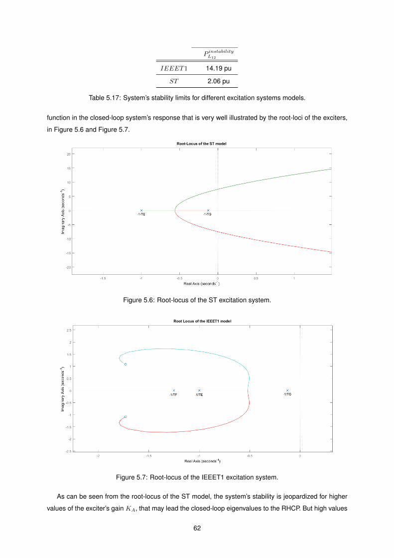
P instabilityL12
IEEET1 14.19 pu
ST 2.06 pu
Table 5.17: System’s stability limits for different excitation systems models.
function in the closed-loop system’s response that is very well illustrated by the root-loci of the exciters,
in Figure 5.6 and Figure 5.7.
Figure 5.6: Root-locus of the ST excitation system.
Figure 5.7: Root-locus of the IEEET1 excitation system.
As can be seen from the root-locus of the ST model, the system’s stability is jeopardized for higher
values of the exciter’s gain KA, that may lead the closed-loop eigenvalues to the RHCP. But high values
62

of KA are needed in order to minimize the steady-state error following a change in the AVR reference
and for a proper and fast dynamic response of the AVR [22].
Introducing the retro-active stabilizing loop changes the root-locus as pictured in Figure 5.7, allowing
for higher values of KA without risking the system’s stability.
Effect of Gain KA
As mentioned in section 2.2.3, reduction in damping is proportional to the AVR gain KA. In a system
whose stability limits are dictated by electromechanical oscillations, which arise due to lack of damping,
increasing KA should decrease stability margins.
Tables 5.18 to 5.20 reflect this tendency, showing how P instabilityL12decreases as KA rises. The
IEEET1 excitation system was chosen to test this effect.
Machine 1 2 3 4 5 6 7 8 9 10
KA 0 6.2 5 5 40 5 40 5 40 5
P instabilityL12= 14.19 pu
Table 5.18: P instabilityL12for the original values of KA.
Machine 1 2 3 4 5 6 7 8 9 10
KA 0 100 100 100 100 100 100 100 100 100
P instabilityL12= 13.30 pu
Table 5.19: P instabilityL12when KA is increased to 100 for every generating unit.
Machine 1 2 3 4 5 6 7 8 9 10
KA 0 200 200 200 200 200 200 200 200 200
P instabilityL12= 10.92 pu
Table 5.20: P instabilityL12when KA is increased to 200 for every generating unit.
5.2.2 PSS Effect
To study the PSS effect on the 10-machine 39-bus network the ST excitation system is chosen because
it shortens the system’s stability limits the most. The excitation system parameters KA and TA are as
presented in Table E.2 of Appendix E.
The system is characterized by fifty eigenvalues, twenty of them corresponding to ten swing modes
that are presented in Table 5.21.
The swing mode λ1,2 is in the RHCP and so the system is unstable at the nominal operation with
PL12= 2.06 pu. Since the power-flow only diverges at PL12
= 18.24 pu there is much potential for
63
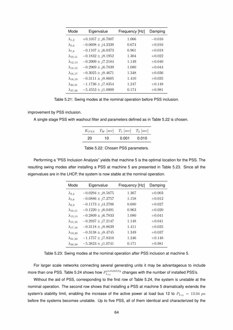
Mode Eigenvalue Frequency [Hz] Damping
λ1,2 +0.1057± j6.7007 1.066 −0.016
λ5,6 −0.0698± j4.2339 0.674 +0.016
λ7,8 −0.1107± j6.0373 0.961 +0.018
λ10,11 −0.1832± j8.1952 1.304 +0.022
λ12,13 −0.2909± j7.2184 1.149 +0.040
λ14,15 −0.2969± j6.7839 1.080 +0.044
λ16,17 −0.3025± j8.4671 1.348 +0.036
λ18,19 −0.3111± j8.8605 1.410 +0.035
λ30,31 −1.1736± j7.8354 1.247 +0.148
λ37,38 −5.4553± j1.0909 0.174 +0.981
Table 5.21: Swing modes at the nominal operation before PSS inclusion.
improvement by PSS inclusion.
A single stage PSS with washout filter and parameters defined as in Table 5.22 is chosen.
KPSS TW [sec] T1 [sec] T2 [sec]
20 10 0.001 0.010
Table 5.22: Chosen PSS parameters.
Performing a ”PSS Inclusion Analysis” yields that machine 5 is the optimal location for the PSS. The
resulting swing modes after installing a PSS at machine 5 are presented in Table 5.23. Since all the
eigenvalues are in the LHCP, the system is now stable at the nominal operation.
Mode Eigenvalue Frequency [Hz] Damping
λ3,4 −0.0294± j8.5875 1.367 +0.003
λ5,6 −0.0886± j7.2757 1.158 +0.012
λ8,9 −0.1173± j4.2706 0.680 +0.027
λ10,11 −0.1220± j6.0491 0.963 +0.020
λ13,14 −0.2809± j6.7833 1.080 +0.041
λ15,16 −0.2937± j7.2147 1.148 +0.041
λ17,18 −0.3118± j8.8639 1.411 +0.035
λ19,20 −0.3138± j8.4745 1.349 +0.037
λ31,32 −1.1757± j7.8310 1.246 +0.148
λ38,39 −5.3823± j1.0741 0.171 +0.981
Table 5.23: Swing modes at the nominal operation after PSS inclusion at machine 5.
For larger scale networks connecting several generating units it may be advantageous to include
more than one PSS. Table 5.24 shows how P instabilityL12changes with the number of installed PSS’s.
Without the aid of PSS, corresponding to the first row of Table 5.24, the system is unstable at the
nominal operation. The second row shows that installing a PSS at machine 5 dramatically extends the
system’s stability limit, enabling the increase of the active power at load bus 12 to PL12= 13.04 pu
before the systems becomes unstable. Up to five PSS, all of them identical and characterized by the
64

Machine
1 2 3 4 5 6 7 8 9 10 P instabilityL12
- - - - - - - - - - 2.06 pu
- - - - X - - - - - 13.04 pu
- X - - X - - - - - 13.24 pu
- X - - X - - - - X 13.30 pu
- X - - X - - - X X 13.45 pu
- X - - X - X - X X 13.78 pu
- X - - X - X X X X 13.79 pu
Table 5.24: Effect of including multiple PSS’s on system’s stability.
parameters in Table 5.22, are successively installed, each time increasing P instabilityL12. However, these
successive increases of P instabilityL12are not as substantial when compared with the first PSS at machine
5. The investment of multiple PSS may not be economically attractive.
65

66

Chapter 6
Conclusions
In this final chapter the goal of the thesis is recalled, a summary of the achievements is presented, the
main difficulties encountered throughout the course of the work are referenced and some proposals for
future work are listed.
6.1 Achievements
The proposed goal of the thesis was to complement a MATLAB-based power system small signal anal-
ysis program called MaSSA with a ”PSS Inclusion Study” option that would allow the user to simulate
the impact of including a PSS in a given network. To achieve this, the problem was partitioned into three
objectives: to include the PSS dynamics in MaSSA; to establish the criteria for optimal PSS location and
to establish the criteria for optimal PSS tuning.
The first course of action was to implement the PSS dynamics in MaSSA. In order to do so, it was
necessary to determine the PSS structure as well as its input signal. To be aligned with most of the
literature, normalized shaft speed deviations ∆ν was the chosen PSS input signal. It was decided that
the PSS would have a somewhat flexible structure, and so the user may choose to have either a single-
stage or a two-stage phase compensation. Including a washout filter is also optional.
Once these PSS characteristics were settled it became possible to mathematically describe the PSS
dynamics, defined by one, two or three differential equations, depending on the chosen PSS structure.
In order to integrate the PSS dynamics in MaSSA, the obtained differential equations were linearized.
This is valid because the scope of MaSSA is confined to small signal analysis.
Finally, the linearized PSS equations are, in a modular way, unified with the existing differential-
algebraic equations model that describes the power system. MaSSA now accommodates the possibility
of including PSS in a given network. ”PSS Inclusion Study” is equipped with the functionalities to print
the ”Eigenvalues of the Original System” and to print the ”Eigenvalues of the Compensated System”,
allowing a modal analysis of the effect that the PSS has on the power system.
The first approach to determining the optimal location for the PSS was by adopting a technique
named OPLI and proposed in [19]. This technique states that the optimal machine to install the PSS
67

is the machine whose AVR’s frequency response changes the most by the influence of the PSS. Even
after some customized adjustments, this approach when implemented and tested in MaSSA proved to
be fallible in some situations and so optimal PSS location could not be solely relied on it.
Ultimately, it was settled that the criterion for optimal location would be the ability to improve the
system’s power transfer capability. That is, the optimal machine is the one that allows the heaviest
loading conditions without leading the system to instability.
For either of the presented approaches it is necessary to install the PSS at each machine at a time
and then compare performances between machines.
”PSS Inclusion Study” is equipped with a ”OPLI” functionality and a ”Power Transfer Improvement”
functionality that compute which should be the optimal machine to install the PSS.
Optimizing the PSS tuning concerns choosing values for the PSS parameters TW , T1, T2, T3, T4 and
KPSS that satisfy the tuning criteria the best.
The tuning criteria for the washout filter is that its transfer function should be approximately unitary
for the range of frequencies in which it is desirable the PSS to perform. In general, this is satisfied by
setting TW = 10 sec.
The tuning criteria for the PSS gain KPSS is that it should be approximately one third of the PSS gain
that leads the system to instability. ”PSS Inclusion Study” is equipped with a ”Perform a Gain Margin
Test” functionality which iteratively and interactively allows the user to conclude about the instability gain.
To establish and to implement the tuning criteria for the phase compensation time constants T1,
T2, T3 and T4 was the most challenging task of the thesis. The typical approach to PSS design is by
recurring to the Heffron-Phillips SMIB representation. This thesis deals not with the single machine
connected to an infinite bus case but with multiple interconnected machines. Nevertheless, the analysis
and conclusions inferred from SMIB can be extended to the multimachine scenario.
The tuning criteria for the time constants is that the lead-lag blocks should compensate fo the phase-
lag introduced by the generator, the excitation system and the power system. In the SMIB case this is
very straightforward, since there is only one generator and one excitation system. In a multimachine
scenario, the machines are electrically interconnected by the non-linear power-flow equations. The
sources of the phase-lag that the PSS should compensate for are not easily identifiable or separable.
It was settled that the time constants T1, T2, T3 and T4 should be such that they compensate for
the phase-lag of the transfer function ∆T stabe
∆ν , computed for the machine in which the PSS is installed.
This transfer function is obtained by visualizing the machine as an Heffron-Phillips SMIB model but
because it is computed at the expenses of the system matrix Asys, it accounts for the inter-relations of
the multimachine power system that are underlying in Asys.
”PSS Inclusion Study” presents the user with the Bode diagrams of the relevant transfer functions
needed to perform the tuning of the time constants.
A further accomplishment was the addition to MaSSA of a reduced order synchronous machine
model commonly known as the Flux-Decay model and named GENDEC. This model is widely used
in the referenced bibliography and so its introduction was convenient. This implementation was then
compared with the Power System Toolbox and successfully validated.
68

Three examples of power systems that benefited from the inclusion of PSS were simulated in MaSSA,
corroborating that the proposed initial objectives for the thesis were accomplished. In this testing phase,
it was found that some of the previously existing data files did not yield reasonable eigenvalues, regard-
less of considering or not the PSS. This setback allowed to discover some constraints in the elaboration
of the data files that were not previously detailed in the instructions MaSSA.
Testing the implemented methodology in the three networks yielded the following conclusions:
• Installing a PSS will only improve the system’s stability margins if these margins are limited by the
presence of local mode or inter-area mode electromechanical oscillations.
• A PSS installed in a machine that is not the main responsible for instability will have no significant
effect in improving stability margins. The PSS location is crucial in its performance.
• The machine mainly responsible for instability is probably the machine that contributes the most to
the participation factors of the electromechanical oscillation limiting the stability. It is likely that this
machine will be the best candidate for PSS site.
• A poorly tuned PSS may deteriorate the system’s stability even more. The PSS tuning is crucial in
its performance.
• OPLI indicates which AVR is the most sensitive to the impact of PSS, but it does not discern
whether this impact is favourable or detrimental.
• OPLI is based on the change of response of the AVR as the critical swing mode moves in the
complex plane. However, the identification of the displaced critical swing mode is not always
trustworthy.
• The load elasticity influences the system’s stability, regardless of having or not a PSS installed.
Constant power is consistently the least favourable scenario but there is no observable trend when
comparing constant current and constant impedance.
• The strength of the connection between power systems influences the system’s oscillatory stability.
Reducing the number of tie lines between areas weakens the connection and arises inter-area
modes of oscillation. Installing a PSS damps these oscillations, extending the stability limits even
in the case of loss of lines.
• The amount of power transfer between power systems influences the system’s oscillatory stability.
The heavier the power transfer between connected generating areas, the more prone the system
is to the rise of inter-area modes of oscillation. Installing a PSS can significantly damp these
oscillations of concern.
• The ST AVR model significantly reduces the stability margins when compared to the IEEET1
model. This is aggravated for higher values of the AVR gain KA. Installing a PSS when using
a ST AVR can compensate this problem and allows higher values of KA.
69

• Installing multiple PSS may not be economically attractive, depending on the improvement that
they introduce on power transfer capability.
• In the *.raw data files the first declared bus has to be swing bus. The following have to be the PV
buses and only then come the PQ buses. Furthermore, the buses have to numbered following this
order.
• In the *.dyr data files the first declared dynamic elements have to be the ones corresponding to
the swing bus, numbered 1. The next dynamic elements have to be the ones corresponding to bus
numbered 2, and so on in increasing order.
6.2 Future Work
Although the goal of the thesis was broadly accomplished, there are some unexplored features that can
be a starting point to expand MaSSA in the future.
Since it was not relevant for the scope of the developed work, turbine-governor control system action
was neglected. Turbine-governors perform load-frequency control, that is, when load demand changes
the mechanical power and the electric active power are no longer balanced, slowing down or accelerating
the machine’s speed, ergo the system’s frequency. Turbine-governors open (close) the admission valves
allowing an increase (decrease) of the mechanical power, ensuring that the machine’s speed remains
close to the synchronous speed. Hence, introducing turbine-governor action may eliminate the need for
PSS in certain situations.
Including turbine-governor action along with PSS action implies implementing a torsional filter in the
PSS structure, to prevent the PSS of interacting with possible turbine-generator shaft torsional oscilla-
tions. Such interaction could lead to shaft damage as well as saturation of the PSS output and of the
AVR [18].
MaSSA is prepared to incorporate a PSS with either one or two lead-lag stages. This should be
sufficient since most of the phase-lag is introduced by the AVR, which can be either ST introducing
90◦ of phase-lag, or it can be IEEET1 introducing 180◦ of phase-lag. Nevertheless, in order to better
resemble real networks and anticipating the addition of new AVR models in the code, it is suggested that
the code could be adapted to accommodate more lead-lag stages.
The topic of adaptive control for PSS design was mentioned in section 2.3.2. It is suggested as
future work to determine in which conditions the effort of adaptive control may be justified and if so,
which would be the best approach/method to implement it. Section 3.7 of [15] briefly describes some
adaptive control methods: MRAC (Model Reference Adaptive Control), STR (Self-Tuning Regulators)
and GSC (Gain Scheduling Controllers).
Another step in the evolution of MaSSA is the inclusion of renewable energy dynamic models like
wind generators and their respective controllers, improving MaSSA’s ability to simulate realistic net-
works.
70

Bibliography
[1] P. Kundur. Power System Stability And Control. McGraw-Hill, 1994.
[2] P. Araujo. Dynamic simulations in realistic-size networks. Master’s thesis, Instituto Superior
Tecnico, Technical University of Lisbon, 2010.
[3] C. Anjos. Optimal location of facts for the enhancement of power system security-the eigenvalues
approach. Master’s thesis, Instituto Superior Tecnico, Technical University of Lisbon, 2011.
[4] M. Seabra. Analise de estabilidade para pequenas perturbacoes. Master’s thesis, Instituto Superior
Tecnico, Technical University of Lisbon, 2013.
[5] M. Trindade. Optimal location of facts to optimize power system security. Master’s thesis, Instituto
Superior Tecnico, Technical University of Lisbon, 2013.
[6] P. Kundur, J. Paserba, and V. Ajjarapu. Definition and classification of power system stability. IEEE
Transactions on Power Systems, Vol. 19(No. 2), May 2004.
[7] E. V. Larsen and D. Swann. Applying power system stabilizers part ii: Performance objectives and
tuning concepts. IEEE Transactions on Power Apparatus and Systems, Vol. PAS-100, June 1981.
[8] task Force 07 of Advisory Group 01 of Study Committee 38. Analysis and control of power system
oscillations. Technical Brochure 111, CIGRE, December 1996.
[9] B. Pal and B. Chaudhuri. Robust Control in Power Systems. Springer US, 2005. DOI
10.1007/b136490.
[10] G. Gajjar and S. A. Soman. Power system oscillation modes identifications: Guidelines for applying
tls-esprit method. IEEE, December 2012.
[11] P. W. Sauer and M. A. Pai. Power System Dynamics and Stability. Prentice Hall, 1997. ISBN:978-
81-7319-594-5.
[12] F. de Mello and C. Concordia. Concepts of synchronous machine stability as affected by excitation
control. IEEE, PAS-88(4), April 1969.
[13] Heffron and Phillips. Effect of a modern amplidyne voltage regulator on underexcited operation of
large turbine generators. AIEE, August 1952.
71

[14] H. Wang and W. Du. Analysis and Damping Control of Power System Low-frequency Oscillations.
Springer, 2016.
[15] M. A. Pai, D. P. S. Gupta, and K. R. Padiyar. Small Signal Analysis of Power Systems. Narosa,
2004. ISBN:978-81-7319-594-5.
[16] E. V. Larsen and D. Swann. Applying power system stabilizers part i: General concepts. IEEE
Transactions on Power Apparatus and Systems, Vol. PAS-100, June 1981.
[17] P. Kundur, M. Klein, G. J. Rogers, and M. S. Zywno. Application of power system stabilizers for
enhancement of overall system stability. IEEE Transactions on Power Systems, Vol. 4(No. 2), May
1989.
[18] E. V. Larsen and D. Swann. Applying power system stabilizers part iii: Practical considerations.
IEEE Transactions on Power Apparatus and Systems, Vol. PAS-100, June 1981.
[19] D. Mondal, A. Chakrabarti, and A. Sengupta. Selection of optimum location of power system stabi-
lizer in a multimachine power system. Journal of Electrical and Electronics Engineering Research,
Vol.2(1):001–013, February 2010. ISSN–2141–2367.
[20] E. J. R. Morgado. Controlo de sistemas dinamicos - uma introducao. 2012.
[21] D. R. Morris. Analysis of low frequency oscillations in power systems. Master’s thesis, University of
Illinois at Urbana-Champaign, 1994.
[22] J. P. S. Paiva. Redes de energia electrica: uma analise sistemica. IST Press, 2007.
[23] M. A. Pai. Energy Function Analysis for Power System Stability. Springer, 1989.
[24] Program Application Guide, Volume II. Siemens, 2010.
72

Appendix A
Dynamic Models
The block diagrams of the dynamic models available in MaSSA are here presented. The respective
equations are only shown for the models that were used throughout the thesis.
A.1 Synchronous Machine
GENROE Model
GENROE is a round rotor synchronous machine model with exponential saturation in the d-q axis.
Its mathematical description, consisting of six differential equations and two algebraic stator equa-
tions, can be consulted in [5]. Figure A.3 is the block diagram representation of the linearized GENROE
equations.
GENRED Model
GENRED is a particular case of the GENROE model that is obtained by neglecting both stator and
network transients as well as saturation. Equations A.1 to A.6 mathematically describe GENRED. This
model is also known as the two-axis model in [11].
dδ
dt= ω − ωs (A.1)
dω
dt= −
(E′q −X ′dId)M
Iq −(E′d +X ′qIq)
MId −
D
M(ω − ωs) +
TMM
(A.2)
dE′qdt
= −E′qT ′d0
− (Xd −X ′d)T ′d0
Id +EfdT ′d0
(A.3)
dE′ddt
= − E′d
T ′q0+
(Xq −X ′q)T ′q0
Iq (A.4)
E′d − V sin(δ − θ)−RsId +X ′qIq = 0 (A.5)
E′q − V cos(δ − θ)−RsIq +X ′dId = 0 (A.6)
73

Figure A.1: Block diagram representation of the GENROE model, reprinted from [24].
GENSAL Model
GENSAL is a salient pole synchronous machine with quadratic saturation in d-axis.
Its mathematical description, consisting of five differential equations and two algebraic stator equa-
tions, can be consulted in [4]. Figure A.2 is the block diagram representation of the linearized GENSAL
equations.
A.2 Excitation System
The excitation system regulates the excitation voltage and is therefore called automatic voltage regulator
and sometimes is referred to simply as exciter.
IEEET1 Model
IEEET1 is a DC type of exciter, defined by equations A.7 to A.9.
74

Figure A.2: Block diagram representation of the GENSAL model, reprinted from [24].
Figure A.3 is the block diagram representation of the linearized IEEET1 equations.
TEdEfddt
= −(KE + SE(Efd))Efd + VR (A.7)
TFdRFdt
= −RF +KF
TFEfd (A.8)
TAdVRdt
= −VR +KARF−KAKF
TFEfd +KA(Vref − V + Vs) (A.9)
ST Model
ST is a static type of exciter, defined by equation A.10.
Figure A.4 is the block diagram representation of the linearized ST equation.
TAdEfddt
= −Efd +KA(Vref − V + Vs) (A.10)
75

Figure A.3: Block diagram representation of IEEET1, adapted from [11].
Figure A.4: Block diagram representation of ST, adapted from [11].
A.3 Turbine-Governor System
TGOV1 Model
TGOV1 is a simple model representing governor action and the reheater time constant effect for a steam
turbine [24].
Figure A.5 is a block diagram representation of the linearized TGOV1 model.
Figure A.5: Block diagram representation of the TGOV1 model, reprinted from [24].
76

HYGOV Model
HYGOV represents a straightforward hydro electric plant governor [24].
Figure A.6 is a block diagram representation of the linearized HYGOV model.
Figure A.6: Block diagram representation of the HYGOV model, reprinted from [24].
GAST Model
GAST represents the principal dynamic characteristics of industrial gas turbines driving generators con-
nected to electric power systems [24].
Figure A.7 is a block diagram representation of the linearized GAST model.
Figure A.7: Block diagram representation of the GAST model, reprinted from [24].
77

Appendix B
WSCC 3-machine 9-bus System
Figure B.1: WSCC 3-machine 9-bus system, reprinted from [19].
78

Bus no Bus type V oltage[pu] PG[pu] QG[pu] PL[pu] QL[pu]
1 swing 1.040 0.716 0.270 − −2 PV 1.025∠ + 9.3◦ 1.630 0.067 − −3 PV 1.025∠ + 4.7◦ 0.850 −0.109 − −4 PQ 1.026∠− 2.2◦ − − − −5 PQ 0.996∠− 4.0◦ − − 1.250 0.500
6 PQ 1.013∠− 3.7◦ − − 0.900 0.300
7 PQ 1.026∠ + 3.7◦ − − − −8 PQ 1.016∠ + 0.7◦ − − 1.000 0.350
9 PQ 1.032∠ + 2.0◦ − − − −
Table B.1: WSCC 3-machine 9-bus system power-flow on the 100 MVA base.
Machine 1 Machine 2 Machine 3
T ′d0[sec] 8.96 6.00 5.89
H[sec] 23.64 6.40 3.01
D[pu] 0.0254 0.0066 0.0026
Xd[pu] 0.1460 0.8958 1.3125
Xq[pu] 0.0608 0.1198 0.1813
X ′d[pu] 0.0608 0.1198 0.1813
Table B.2: WSCC 3-machine 9-bus system machine data on the 100 MVA base.
Exciter 1 Exciter 2 Exciter 3
TA[sec] 0.2 0.2 0.2
KA 175 175 175
Table B.3: WSCC 3-machine 9-bus system excitation data on the 100 MVA base.
79

Appendix C
GENDEC Machine Model
C.1 Equations
• Differential Equationsdδ
dt= ω − ωs (C.1)
dω
dt= −D
M(ω − ωs)−
E′qIq
M− (Xq −X ′d)
MIdIq +
TMM
(C.2)
dE′qdt
= −E′qT ′d0
+EfdT ′d0
− (Xd −X ′d)T ′d0
Id (C.3)
• Stator Algebraic Equations
V sin(δ − θ) +RsId −XqIq = 0 (C.4)
E′q − V cos(δ − θ)−RsIq −X ′dId = 0 (C.5)
C.2 Linearization
• Linearized Differential Equations
∆δ = ∆ω (C.6)
∆ω = −DM
∆ω − Iq0M
∆E′q −(E′q0M
+ Id0(Xq −X ′d)
M
)∆Iq − Iq0
(Xq −Xd)
M∆Id +
∆TMM
(C.7)
∆E′q = − 1
T ′d0
∆E′q +1
T ′d0
∆Efd −(Xd −X ′d)
T ′d0
∆Id (C.8)
• Linearized Stator Algebraic Equations
V0cos(δ0 − θ0)∆δ +Rs∆Id −Xq∆Iq − V0cos(δ0 − θ0)∆θ + sin(δ0 − θ0)∆V = 0 (C.9)
V0sin(δ0 − θ0)∆δ + E′q −X ′d∆Id −Rs∆Iq − V0sin(δ0 − θ0)∆θ − cos(δ0 − θ0)∆V = 0 (C.10)
80

Appendix D
Two-Area System
Bus no Bus type V oltage[pu] PG[pu] QG[pu] PL[pu] QL[pu]
1 swing 1.03 7.2172 1.4462 − −2 PV 1.01∠− 1.50◦ 7.0000 1.5940 − −3 PV 1.03∠ + 8.22◦ 7.0000 1.3393 − −4 PV 1.01∠− 10.20◦ 7.0000 1.8070 − −5 PQ 1.01∠ + 3.66◦ − − − −6 PQ 0.99∠− 6.24◦ − − − −7 PQ 1.01∠− 4.70◦ − − − −8 PQ 0.98∠− 14.94◦ − − − −9 PQ 0.98∠− 14.42◦ − − 11.590 −0.7350
10 PQ 0.97∠− 23.29◦ − − 15.750 −0.8990
Table D.1: Two-area system power-flow on the 100 MVA base.
Machine 1 Machine 2 Machine 3 Machine 4
T ′d0[sec] 8.00 8.00 8.00 8.00
T ′q0[sec] 0.40 0.40 0.40 0.40
H[sec] 63.0 54.0 54.0 63.0
D[pu] 0.0 0.0 0.0 0.0
Xd[pu] 0.20 0.20 0.20 0.20
Xq[pu] 0.19 0.19 0.19 0.19
X ′d[pu] 0.033 0.033 0.033 0.033
X ′q[pu] 0.061 0.061 0.061 0.061
Table D.2: Two-area system machine data on the 100 MVA base.
Exciter 1 Exciter 2 Exciter 3 Exciter 4
TA[sec] 0.1 0.1 0.1 0.1
KA 200 200 200 200
Table D.3: Two-area system excitation data on the 100 MVA base.
81

From Bus To Bus Resistance[pu] Reactance[pu] Shunt Susceptance[pu]
1 5 0.001 0.012 0.000
2 6 0.001 0.012 0.000
9 10 0.022 0.220 0.330
9 10 0.022 0.220 0.330
9 10 0.022 0.220 0.330
9 6 0.002 0.020 0.030
9 6 0.002 0.020 0.030
3 7 0.001 0.012 0.000
4 8 0.001 0.012 0.000
10 8 0.002 0.020 0.030
10 8 0.002 0.020 0.030
5 6 0.005 0.050 0.075
5 6 0.005 0.050 0.075
7 8 0.005 0.050 0.075
7 8 0.005 0.050 0.075
Table D.4: Two-area system transmission line data on the 100 MVA base.
82

Appendix E
New England 10-machine 39-bus
System
T ′d0[sec] T ′q0[sec] H[sec] D[pu] Xd[pu] Xq[pu] X ′d[pu] X ′q[pu]
Machine 1 7.00 0.70 500 0 0.0200 0.019 0.0060 0.0080
Machine 2 6.56 1.50 30.3 0 0.2950 0.282 0.0697 0.1700
Machine 3 5.70 1.50 35.8 0 0.2495 0.237 0.0531 0.0876
Machine 4 5.69 1.50 28.6 0 0.2620 0.258 0.0436 0.1660
Machine 5 5.40 0.44 26.0 0 0.6700 0.620 0.1320 0.1660
Machine 6 7.30 0.40 34.8 0 0.2540 0.241 0.0500 0.0814
Machine 7 5.66 1.50 26.4 0 0.2950 0.292 0.0490 0.1860
Machine 8 6.70 0.41 24.3 0 0.2900 0.280 0.0570 0.0911
Machine 9 4.79 1.96 34.5 0 0.2106 0.205 0.0570 0.0587
Machine 10 10.2 0.10 42.0 0 0.1000 0.069 0.0310 0.0080
Table E.1: New England 10-machine 39-bus system machine data on the 100 MVA base.
TA[sec] KA
Exciter 1 0.05 0
Exciter 2 0.05 6.2
Exciter 3 0.06 5.0
Exciter 4 0.06 5.0
Exciter 5 0.02 5.0
Exciter 7 0.02 40
Exciter 8 0.02 5.0
Exciter 9 0.02 40
Exciter 10 0.06 5.0
Table E.2: New England 10-machine 39-bus system excitation data on the 100 MVA base.
83

Figure E.1: 10-machine 39-bus system, adapted from [23].
84

Bus no Bus type V oltage[pu] PG[pu] QG[pu] PL[pu] QL[pu]
1 swing 1.03 15.242 0.9186 11.04 2.50
2 PV 1.03∠ + 9.47◦ 8.3000 0.2737 − −3 PV 1.03∠ + 4.81◦ 5.4000 0.1029 − −4 PV 1.06∠ + 8.92◦ 5.6000 1.0288 − −5 PV 1.05∠ + 6.22◦ 6.5000 2.1542 − −6 PV 1.01∠ + 3.76◦ 5.0800 1.6700 − −7 PV 1.00∠ + 4.79◦ 6.3200 1.1259 − −8 PV 0.98∠ + 1.32◦ 6.5000 2.1025 − −9 PV 0.98∠− 9.93◦ 0 1.6774 0.046
10 PV 1.05∠− 0.72◦ 2.5000 1.4994 − −11 PQ 1.05∠ + 2.40◦ − − 2.835 0.269
12 PQ 1.05∠− 0.36◦ − − 2.060 0.276
13 PQ 1.04∠− 6.19◦ − − 2.810 0.755
14 PQ 1.05∠− 3.88◦ − − 1.390 0.170
15 PQ 1.06∠− 1.99◦ − − 2.240 0.472
16 PQ 1.04∠− 5.48◦ − − 3.086 −0.922
17 PQ 1.04∠ + 1.06◦ − − 2.475 0.846
18 PQ 1.05∠ + 1.26◦ − − − −19 PQ 1.03∠− 3.19◦ − − 2.740 1.150
20 PQ 0.99∠− 1.43◦ − − 6.280 1.030
21 PQ 1.05∠− 0.43◦ − − − −22 PQ 1.03∠− 7.19◦ − − 1.580 0.300
23 PQ 1.03∠− 6.39◦ − − − −24 PQ 1.03∠− 5.60◦ − − 3.290 0.323
25 PQ 1.01∠− 7.51◦ − − 3.200 1.530
26 PQ 1.01∠− 8.26◦ − − − −27 PQ 1.01∠− 7.18◦ − − − −28 PQ 1.00∠− 7.51◦ − − 0.075 0.880
29 PQ 1.01∠− 7.73◦ − − − −30 PQ 1.02∠− 6.69◦ − − − −31 PQ 1.02∠− 4.49◦ − − − −32 PQ 0.99∠− 11.14◦ − − 5.220 1.760
33 PQ 1.00∠− 11.09◦ − − 2.338 0.840
34 PQ 1.01∠− 9.79◦ − − − −35 PQ 1.00∠− 10.05◦ − − − −36 PQ 1.00∠− 10.11◦ − − 5.000 1.840
37 PQ 1.03∠− 7.38◦ − − 3.220 0.024
38 PQ 1.05∠− 3.14◦ − − − −39 PQ 1.05∠− 1.23◦ − − − −
Table E.3: New England 10-machine 39-bus power-flow on the 100 MVA base.
85

From Bus To Bus Resistance[pu] Reactance[pu] Shunt Susceptance[pu]
39 38 0.0035 0.0411 0.6987
39 1 0.0010 0.0250 0.7500
38 37 0.0013 0.0151 0.2572
38 15 0.0070 0.0086 0.1460
37 36 0.0013 0.0213 0.2214
37 22 0.0011 0.0133 0.2138
36 35 0.0008 0.0128 0.1342
36 26 0.0008 0.0129 0.1382
35 34 0.0002 0.0026 0.0434
35 32 0.0008 0.0112 0.1476
34 33 0.0006 0.0092 0.1130
34 29 0.0007 0.0082 0.1389
33 32 0.0004 0.0046 0.0780
32 31 0.0023 0.0363 0.3804
31 1 0.0010 0.0250 1.2000
30 29 0.0004 0.0043 0.0729
30 27 0.0004 0.0043 0.0729
27 26 0.0009 0.0101 0.1723
26 25 0.0018 0.0217 0.3660
25 24 0.0009 0.0094 0.1710
24 23 0.0007 0.0089 0.1342
24 21 0.0016 0.0195 0.3040
24 19 0.0008 0.0135 0.2548
24 16 0.0003 0.0059 0.0680
23 22 0.0007 0.0082 0.1319
23 13 0.0013 0.0173 0.3216
19 18 0.0008 0.0140 0.2565
18 17 0.0006 0.0096 0.1846
17 16 0.0022 0.0350 0.3610
15 14 0.0032 0.0323 0.5130
14 13 0.0014 0.0147 0.2396
14 12 0.0043 0.0474 0.7802
14 11 0.0057 0.0625 1.0290
12 11 0.0014 0.0151 0.2490
28 29 0.0016 0.0435 0.0000
28 27 0.0016 0.0435 0.0000
34 9 0.0000 0.0250 0.0000
30 8 0.0000 0.0200 0.0000
21 7 0.0007 0.0142 0.0000
20 6 0.0009 0.0180 0.0000
18 5 0.0000 0.0143 0.0000
17 4 0.0005 0.0272 0.0000
15 3 0.0006 0.0232 0.0000
38 10 0.0000 0.0181 0.0000
11 2 0.0008 0.0156 0.0000
21 20 0.0007 0.0138 0.0000
Table E.4: New England 10-machine 39-bus system transmission line data on the 100 MVA base.
86

Appendix F
Combinations of models implemented
in MaSSA
Figure F.1 represents every possible combination between models available in MaSSA.
In Figure F.1, only the coloured blocks correspond to the implemented combinations. The blue blocks
represent the four existing synchronous machine models, the orange blocks represent the AVR models
and the grey blocks the turbine-governor models.
Because the PSS acts by means of the AVR, it is unreasonable to implement the PSS in machines
without excitation control and thus such combinations are disregarded.
87

Figure F.1: Combinations of models implemented in MaSSA.
88


![Download [5.17 MB]](https://static.fdocuments.in/doc/165x107/586768a71a28ab52568b4d21/download-517-mb.jpg)