
Optimal Life-Cycle Strategies in the Presence of Interest ... · PDF fileOptimal Life-Cycle...
31
Optimal Life-Cycle Strategies in the Presence of Interest Rate and Inflation Risk Raimond H. Maurer, Christian Schlag and Michael Z. Stamos October 2007 PRC WP2008-01 Pension Research Council Working Paper Pension Research Council The Wharton School, University of Pennsylvania 3620 Locust Walk, 3000 SH-DH Philadelphia, PA 19104-6302 Tel: 215.898.7620 Fax: 215.573.3418 Email: [email protected] http://www.pensionresearchcouncil.org This research was conducted with support from the German Research Foundation (DFG) and the German Investment and Asset Management Association (BVI). Opinions and errors are solely those of the author and not of the institutions with whom the authors are affiliated. © 2007 R.H. Maurer, C. Schlag, and M.Z. Stamos. All Rights Reserved. All findings, interpretations, and conclusions of this paper represent the views of the author(s) and not those of the Wharton School or the Pension Research Council. © 2008 Pension Research Council of the Wharton School of the University of Pennsylvania. All rights reserved.
-
Upload
nguyenthuan -
Category
Documents
-
view
217 -
download
0
Transcript of Optimal Life-Cycle Strategies in the Presence of Interest ... · PDF fileOptimal Life-Cycle...

Optimal Life-Cycle Strategies in the Presence of Interest Rate and Inflation Risk
Raimond H. Maurer, Christian Schlag and Michael Z. Stamos
October 2007
PRC WP2008-01 Pension Research Council Working Paper
Pension Research Council The Wharton School, University of Pennsylvania
3620 Locust Walk, 3000 SH-DH Philadelphia, PA 19104-6302
Tel: 215.898.7620 Fax: 215.573.3418 Email: [email protected]
http://www.pensionresearchcouncil.org
This research was conducted with support from the German Research Foundation (DFG) and the German Investment and Asset Management Association (BVI). Opinions and errors are solely those of the author and not of the institutions with whom the authors are affiliated. © 2007 R.H. Maurer, C. Schlag, and M.Z. Stamos. All Rights Reserved. All findings, interpretations, and conclusions of this paper represent the views of the author(s) and not those of the Wharton School or the Pension Research Council. © 2008 Pension Research Council of the Wharton School of the University of Pennsylvania. All rights reserved.

Optimal Life-Cycle Strategies in the Presence ofInterest Rate and Inflation Risk∗
Raimond H. Maurer Christian Schlag Michael Z. Stamos
September 2007
Abstract
The worldwide shift from public pay-as-you-go pension systems to privatelyfunded pension schemes is accompanied by a huge increase in the householdscapital stock mounting to trillions of dollars worldwide which pour into definedcontribution pension plans. In order to assess how these funds should be opti-mally invested, we derive the optimal time-dependent portfolio allocation strategytaking into account long-term stock market, term structure, and inflation risk.Our results confirm that the often advised so-called life-cycle strategy is optimalif non-financial wealth is taken into account. We also benchmark common long-term defined contribution asset allocation strategies relative to the optimum inorder to the assess welfare implications for varying investment horizons and riskaversions. The outcome of utility heavily depends on whether the risk aversionof the investor is estimated appropriately. Misestimation of this parameter andhence wrong investment advice can lead to utility losses of around 60 percent interms of certainty equivalent wealth.
JEL Codes: E21 G11 G23Keywords: Optimal Portfolio Choice, Life-Cycle Asset Alloca-
tion, Defined Contribution Plans.
∗Department of Finance, Goethe University (Frankfurt, Germany), e-mail: [email protected], [email protected], [email protected]. This research was con-ducted with support from the German Research Foundation (DFG) and the German Investment andAsset Management Association (BVI). Opinions and errors are solely those of the author and not ofthe institutions with whom the authors are affiliated. c©2007 R.H. Maurer, C. Schlag, and M.Z. Stamos.All Rights Reserved.

Optimal Life-Cycle Strategies in the Presence ofInterest Rate and Inflation Risk
September 2007
Abstract
The worldwide shift from public pay-as-you-go pension systems to privatelyfunded pension schemes is accompanied by a huge increase in the householdscapital stock mounting to trillions of dollars worldwide which pour into definedcontribution pension plans. In order to assess how these funds should be opti-mally invested, we derive the optimal time-dependent portfolio allocation strategytaking into account long-term stock market, term structure, and inflation risk.Our results confirm that the often advised so-called life-cycle strategy is optimalif non-financial wealth is taken into account. We also benchmark common long-term defined contribution asset allocation strategies relative to the optimum inorder to the assess welfare implications for varying investment horizons and riskaversions. The outcome of utility heavily depends on whether the risk aversionof the investor is estimated appropriately. Misestimation of this parameter andhence wrong investment advice can lead to utility losses of around 60 percent interms of certainty equivalent wealth.
JEL Codes: E21 G11 G23Keywords: Optimal Portfolio Choice, Life-Cycle Asset Alloca-
tion, Defined Contribution Plans.

1 Introduction
The worldwide shift from pay-as-you-go to privately funded pension systems accompa-
nied with the swing from defined benefit schemes to defined contribution plans transfer
both investment risks and responsibility to millions of individual investors. From the
perspective of private investors choosing the right asset allocation seems to be an oner-
ous task. For instance, Rooij, Kool, and Prast (2007) find in an empirical analysis
that households consider themselves financially unsophisticated and are not willing to
take control over their retirement assets.1 According to Huberman, Iyengar, and Jiang
(2004) there exists a strong negative correlation between the number of funds offered in
self directed 401 (k) pension plans and the 401 (k) participation rate. Since individual
plan participants do not seem to understand the risks associated with the various asset
allocation options the present paper aims to derive optimal asset allocation rules which
could serve as default options for defined contribution plans. Beshears et al. (2006)
find a tremendous impact of default options on the outcome of retirement wealth since
financially unsophisticated investors stick to the default option to circumvent serious
investment mistakes.
The default portfolio strategy has to be adequate for a broad range of participants
from a welfare perspective and feasible from the viewpoint of pension plan providers
such as banks, insurance companies, mutual funds, and employers. In order to be prac-
ticable to implement from the plan provider perspective we impose that the optimal
investment strategy only depends on the age and the risk aversion of the plan partic-
ipant. Such a life-cycle strategy seems to be appealing for a variety of reasons. The
simplicity ensures that administrative costs of the plan sponsor are small even if it is
implemented for a large number of plan participants. Further, transaction costs are
1Also psychological studies by Tversky and Shafir (1992), Shafir, Simonson, and Tversky (1993)as well as Iyengar and Lepper (2000) which report that households are inclined to postpone decisionmaking when the complexity of tasks rises.
1

kept at a minimum and excessive active trading is avoided.2 From the view of plan
participants the static life-cycle strategy is transparent and easily comprehensible since
they ex-ante know which asset allocation will be held at future dates. As a result, par-
ticipants can also easily compare different static life-cycle strategies. Life-cycle mutual
funds are one of the most successfully growing segments of the mutual fund industry in
the U.S. The assets under management have grown rapidly from $1 billion in 1996 to
$120 billion in 2006 (Viceira, 2007). Remarkably, president George W. Bush has out-
lined a plan in which workers can invest a portion of their payroll taxes into personal
accounts in exchange for a cut in Social Security benefits. One investment option of
these personal accounts is the life-cycle portfolio.
We have to mention that recent theoretical portfolio choice studies document that
rational investors should trade actively according to stochastic changes of the invest-
ment opportunity set.3 Cairns, Blake, and Dowd (2006) specifically derive the optimal
dynamic asset allocation for defined contribution plans. The derived stochastic life-cycle
strategy exhibits large fluctuations in asset weights over time since hedge demands are
reacting commensurately to the stochastically varying investment opportunity set. It
also exhibits high leveraged stock positions in the beginning of the accumulation plan
since rational investors perceive their human capital as an implicit bond portfolio. The
study also finds that a static life-cycle strategy is significantly suboptimal compared to
its stochastic counterpart. Cocco, Gomez, and Maenhout (2005) provide contradictory
theoretical evidence that utility losses of static life-cycle strategies are vary small com-
pared to the dynamic optimum even theough they do not optimize the static life-cycle
rule. After all, it also seems doubtful whether individual pension plan participants are
2Barber and Odean (2000) find empirical evidence that active trading reduces the investment per-formance of households substantially due to transaction costs and Carhart (1997) finds the same resultfor actively managed mutual funds.
3For instance, the impact of interest rate risk on hedge demands has been analyzed by Brennan andXia (2000) and by Wachter (2003), risky inflation by Campbell and Viceira (2001) and Brennan andXia (2002), and for changing risk premiums see Brandt (1999), Campbell and Viceira (1999), Wachter(2002), and Campbell, Chan, and Viceira (2003).
2

qualified enough to understand optimal stochastic asset allocation strategies and are
willing or allowed to invest into highly leveraged stock portfolios. Another strand of
literature explores the risks associated to typical life-cycle asset allocations rules by
simulating the outcome of retirement wealth via historical simulations. Poterba et al.
(2005) use historical simulations to draw the distribution of 401(k) retirement wealth
for a large number of households and Shiller (2005) uses 134 years of stock return data
for various countries to simulate the outcome of life-cycle personal accounts.
While previous studies did not optimize the static life-cycle asset allocation rules
explicitly we show how static life-cycle strategies can be optimized in a model with
stochastically varying investment opportunity set. We set up a continuous time asset
model which reasonably captures the empirical evidence of multi decade stock market,
interest rate and inflation rate movements and derive the optimal investment schemes
for CRRA plan participants which contribute a certain fraction of their labor income
to a pension plan. Since the resulting static life-cycle strategy evolves deterministically
over time it somehow captures the average development of the investment opportunity
set over time but not the actual state of nature. The strategy exhibits declining equity
exposures until retirement, so as to maintain the optimal stock fraction of total wealth
which includes financial wealth and the present value of future contributions. This result
conforms to recent life-cycle asset allocation studies (e.g. Cocco, Gomes, and Maenhout,
2005) and is similar to popular life-cycle rules suggested by financial advisors or finance
books (Malkiel, 1996).
In order to evaluate the risk associated to the derived optimal static life-cycle strate-
gies we conduct a Monte Carlo analysis to derive distributional properties of terminal
wealth in real terms and of equivalent annuities payments assuming that terminal wealth
is converted into a life-annuity at retirement age. We use the optimal strategy as a
benchmark in order to compare long term investment schemes typically found in prac-
tice such as the constant mix strategy, the ”100−age” life-cycle rule, and the static as
3

well as dynamic portfolio insurance strategies. This allows us to assess the degree of
efficiency of these investment schemes compared to the optimal life-cycle strategy. To
this end, we perform a welfare analysis based on Monte Carlo sampling for the various
strategies, ages, and risk aversions.
The remainder of the paper is structured as follows. In Section 2 we describe the
asset model, its calibration, and derive the wealth evolution equation. Section 3 derives
and discusses the optimal life-cycle strategy. In Section 4 we conduct a Monte Carlo
analysis in order to create projections about potential outcomes of terminal wealth and
pension income. A welfare analysis is also undertaken to compare various practicable
asset allocation strategies relative to the optimum, before Section 5 concludes.
2 The Asset Model
2.1 Stock and Bond Market
This section is concerned with the main long term investment risk factors which private
investors have to cope with: stock market price risk, interest rate risk, and inflation
risk. All considered risk factors are captured by separate stochastic diffusion processes,
each of which can be potentially correlated. The value of the stock market S is assumed
to evolve according to
dSt = (rt + σsλs)Stdt + σsStdZSt , (1)
where rt denotes the short nominal interest rate, σs is the instantaneous standard
deviation of stock returns, λS > 0 represents the market price of equity risk, and ZS
is a Wiener process. So, we assume that the instantaneously expected stock return
is the sum of the prevailing interest rate and the constant risk premium. This way of
modeling ensures that the expected stock return never drops below the risk-free interest
rate.
4

The continuous nominal short rate process is given by Vasiceks (1977) term struc-
ture model
drt = κr(θr − rt)dt + σrdZrt , (2)
where θr denotes the long run mean, κr represents the parameter of mean reversion and
σr is the volatility of the short rate. Mean reversion gives the interest rate a tendency to
move back to the long run mean θr, where the speed factor κr indicates how strong the
force of mean reversion is. The increments of the standardized Wiener processes dZrt
and dZSt are instantaneously correlated with ρSr, which reflects the empirical evidence
of interdependencies between stock returns and interest rates. The value process of the
money market account Kt is given by
dKt = rtKtdt. (3)
To model the dynamics of the bond portfolio, we take advantage of the direct relation
between the movements of the risk-free term structure and bond returns. The dynamics
of the value of the risky bond portfolio B with a given modified duration D = ∂B∂r
1B
follow endogenously from the assumption of the Vasicek model with
dBt(D) = (r + σB(D)λr)Btdt− σB(D)BtdZrt , (4)
where λr > 0 is the market price of interest rate risk and σB(D) = σrD is the instanta-
neous volatility of the bond portfolio.4 Again, the expected return of risky bonds will
always be higher than the current riskless interest rate. For the correlation between
stocks and bonds it holds that ρSB = −ρSr. The (instantaneous) variance-covariance
4The same approach to model the price process of a bond portfolio is used by Munk, Srensen, andVinther (2004).
5

matrix of stocks and bonds is therefore given by
Σ =
σ2S σS σB ρSB
σS σB ρSB σ2B
. (5)
The term structure of zero bond prices in t with maturities τ > 0 is given by
P (t, t + τ) = e−a(τ)−b(τ)rt , (6)
with
a(τ) = R(∞)(τ − b(τ)) +σ2
r
4κb(τ)2,
b(τ) =1
κ(1− e−κτ ),
R(∞) = θ +σrλr
κ− 1
2
σ2r
κ2,
where R(∞) denotes the nominal interest of a zero bond with infinite maturity. De-
pending on the parameter, the Vasicek term structure model can reproduce all types
of empirically observed term structures, i.e. normal, inverse and humped.
2.2 Inflation Risk
We model the inflation rate explicitly because the effect of uncertain inflation becomes
especially important when we consider multi-decade investment horizons. We assume
that the nominal price level of the consumption good evolves according to
dQt = ie,tQtdt + σQQtdZQt , (7)
with ie,t as the expected rate of inflation an σQ the volatility of the unexpected inflation.
The change in the price of the consumption good is correlated with the stock price and
6

the interest rate with ρSQ and ρrQ, respectively. The expected inflation rate itself is
assumed to follow the Ornstein-Uhlenbeck process
die,t = κi(θi − ie,t)dt + σidZit , (8)
where θi describes the long run mean, κi represents the degree of mean reversion, and
σi the volatility of the inflation rate. The correlations between dZSt , dZr
t , dZQt and
dZ it are denoted by ρSi, ρri, and ρQi. This way of modeling the price process of the
consumption good reflects that expected inflation rates are mean reverting over time
which is commensurate to empirical evidence. The result is that possibly there can
be long periods with above average inflation rates and below average inflation rates.
Further, expected inflation rates and interest rates are correlated which is in line with
empirical evidence.
2.3 Calibration of the Asset Model
We use maximum likelihood estimation to calibrate the model parameters to monthly
total return data of the MSCI World performance index, German zero bond spot rates
with maturities τ = 1, 2, ..., 10 years, and the consumer price index from January 1975
to December 2004 (360 observations). The results of the estimation are reported in
Table I. By using the MSCI World performance index we assume that the portion of
funds invested in stocks is internationally diversified. The filtration of the short-rate
and expected inflation is done by applying the Kalman Filter (Figure (1)).5 We set the
modified duration of the bond portfolio to D = 4.5 so that the expected excess return
λrσB is 1.3 percent and volatility σB = Dσr is 3.9 percent. The expected stock excess
return λSσS and the volatility σS are 5.9 and 15.8 percent, respectively. As expected,
the correlation between the expected inflation rate and the interest rate is significant
5For the application of the Kalman Filter to the calibration of the Vasicek model we use theapproach of Babbs and Nowman (1999).
7

0%
2%
4%
6%
8%
10%
12%
1975 1980 1985 1990 1995 2000 2005
Filtered Short Rate Filtered Expected Inflation Rate
Figure 1: Filtered Short Rate and Expected Inflation Rate. The figure exhibits thefiltered annualized short rate and inflation rate computed with the Kalman filter. Theestimation uses monthly data from January 1975 to December 2004 (360 observations).Historical data about the interest rate term structure with maturities τ = 1, 2, ..., 10years and the development of the consumer price index in Germany are taken from thewebsite from the German Central Bank (Bundesbank).
with 57.8 percent. The estimated long run mean of the expected inflation rate θi is 2.4
percent while the long run mean of the nominal short rate is 4.44 percent so that the
real short rate is on average around 2 percent.
3 Optimal Life-Cycle Strategy
3.1 The Wealth Evolution
Having described the risk factors of the economy, we now turn to the evolution of
retirement wealth. We assume that the investor can invest in the stock market, a bond
portfolio with duration D, and the money market. The process of the of the plan
8

Table IKalman Filter Estimates of Asset Model Parameters (in Percent)
Stocks Bonds Interest Rates Inflation Correlations(D = 4.5) S r Q i
λSσS 5.80 λrσB 1.30 θr 4.44 θi 2.40 1 -5.31 -6.75 0.26σS 13.58 σB 3.87 σr 0.86 σi 1.30 1 5.16 52.48
κr 8.07 κi 47.4 1 16.41λr 33.54 σQ 1.01 1
Note. This table reports the (annualized) estimates for the stochastic processes ofstocks, bonds, interest rates and inflation. The estimation uses monthly data fromJanuary 1975 to December 2004 (360 observations). As a proxy for the stock portfoliowe use the return series of the MSCI World performance index. Historical data aboutthe interest rate term structure and the development of the consumer price index inGermany are taken from the website from the German Central Bank (Bundesbank).
member’s nominal wealth is
dF nt = (rt + π′tσλ)F n
t dt + π′tσF nt dZt + ct dt, (9)
where λ = (λS λr)′ is the vector of market prices of risk, σ results from the Cholesky
decomposition Σ = σσ′, and dZt = (dZSt − dZr
t )′. The vector of risky asset portfolio
weights at time t is denoted by πt = (πSt πB
t )′ , where πSt and πB
t reflect the fraction of
retirement wealth invested in stocks and bonds, respectively. Accordingly, the fraction
invested in the money market is given by πCt = 1 − π′t1. The investor continuously
contributes a deterministic amount ct to the retirement wealth account. We assume
that the contribution is 4 percent of a typical employee’s current earnings.6 To this end,
the average earnings profile of an average German employee with vocational training
(Figure (2)) is taken from Fitzenberger et al. (2001). Further, we assume that the
term structure of nominal income rises at 2 percent per year. This increase in nominal
income is chosen conservatively in the way that it compensates for the average increase
of the price level. We abstract from stochastic fluctuations of contributions in order to
6The size of 4 percent is based on German regulations of funded individual retirement accounts(called Riester accounts) which require that from 2008 on 4 percent of income has to be contributedin order to become eligible for the entire tax subsidies.
9

0
5
10
15
20
25
30
35
40
45
25 30 35 40 45 50 55 60 65Age
Labo
r Inc
ome
(Tsd
.)
Figure 2: Average Life-Cycle Earnings Profile. The profile is taken from Fitzenberger etal. (2001) for employees without high school degree but with formal vocational training.Earnings at age 25 are set to 30 thousand EUR per year which is in the line with theaverage earnings of German employees according to the income survey from the FederalStatistical Office of Germany in 2005.
focus on the investment return risks. Cocco, Gomes, and Maenhout (2005) report that
utility costs from ignoring labor income risk are small since the main effect remains in
the discounting of future labor income. The investor’s nominal augmented wealth W nt
consists of the financial wealth F nt and the present value of future contributions Hn
t .
The latter is given by
Hnt =
∫ T
t
csP (t, s− t) ds, (10)
where P (t, s− t) is the price of a zero coupon bond in t with maturity τ = s− t from
equation (6). Hence, the present value of future contributions is equal to a coupon
bond with duration DH,t =∫ T
tcs
∂P (t,s−t)∂rt
ds and dynamics
dHnt = (rt + σH,tλr)H
nt dt− σH,t dZ
rt − ct dt, (11)
10

where σH,t = DH,tσr is the instantaneous volatility. Finally, the dynamics of augmented
wealth after inflation W rt are given by
dW rt = W r
t
{F r
t
W rt
((rt + π′tσλ− π′tσσQ(ρSQ -ρrQ)′) dt + π′tσ dZ
)+
Hrt
W rt
((rt + σH,tλr − σQσH,tρrQ) dt− σH,t dZ
rt
)(12)
+((−ie,t + σ2
Q) dt− σQ dZQt
)}.
Apparently, investors can only control the dynamics of real augmented wealth W rt by
aligning the asset allocation πt of the financial wealth fractionF r
t
W rt, while the dynamics
of the present value of future contributions Ht evolve completely exogenously. Since Hrt
evolves like a coupon bond, the overall stock fraction of W rt is πt
F rt
W rt
< πt. In turn, if
investors desire an x percent overall stock fraction they have to hold, πt = xW r
t
F rt
percent
inside financial wealth. Over time the fractionF r
t
W rt
converges to 1 so that the financial
wealth stock fraction πt decreases to x.
3.2 Optimal Benchmark Strategy
We assume that the individual preferences are described by a utility function of the
constant relative risk aversion class which can be expressed as:
u(W rt ) =
(W rt )1−γ
1− γ, γ > 0, γ 6= 1, (13)
where γ is the individuals coefficient of relative risk aversion (RRA) and T the length
of the investment horizon which is defined as the retirement age 65 minus the age at
which the investor starts to contribute to the pension plan. We will consider invest-
ment horizons of 10, 20, 30, and 40 years, which corresponds to investors starting the
accumulation plan at age 55, 45, 35, and 25, respectively. Note, that at time T the
value of future contributions is 0, so that W rT = F r
T .
11

Since we prevent the portfolio strategy from varying according to the evolution of
state variables, we cannot rely on the standard dynamic asset allocation approach in the
spirit of Merton (1969,1971). Rather than maximizing the drift of the value function
conditional on the current state of nature, we construct the static life-cycle strategy by
deriving the optimal weights πt which maximize the utility drift at each future point in
time given the information at t = 0:
πt = arg max E0
[du(W r
t )], (14)
subject to the intertemporal budget restriction (13). The rationale is that maximizing
the expected utility drift should deliver high terminal utility, as can be seen in the
numerical results of the following section. The advantage of our approach is that the
solution of the optimal asset allocation policy can be derived iteratively for increasing t.
Otherwise it would be necessary to numerically compute the optimal asset allocation for
all dates simultaneously. Due to the extremely high number of choice variables (number
of dates × (number of assets - 1)) the latter approach can easily become numerically in-
stable. To derive the optimal portfolio strategy we need terms of E0[du(W rt )] depending
on πt formed via an application of Ito’s Lemma:
π′tσ
λ− σQ
(1− 1
2γ
) ρSQ
ρ−rQ
E1,t +
1
2γσr
ρSr
−1
E2,t
− 1
2γπ′tσσ′πtE3,t (15)
with
E1,t = E0
[F r
t
(W rt )γ
], E2,t = E0
[DH,t
F rt Hr
t
(W rt )γ+1
], E3,t = E0
[(F r
t )2
(W rt )γ+1
].
12

Computing the first order conditions and solving for the optimal portfolio weights yields
π∗t =1
γE3,t
(σ′)−1
λ− σQ
(1− 1
2γ
) ρSQ
ρ−rQ
E1,t +
1
2γσr
ρSr
−1
E2,t
. (16)
For the calculation of the expectations E1,t, E2,t, and E3,t we perform Monte-Carlo
simulations given the optimal weights for all points in time s with s < t. In case
the semi-analytical solution (16) exhibits short positions, we optimize (14) numerically
given the short-selling restrictions πS, πB, πC ≥ 0. We restrict the investor from short-
selling, since households are usually not allowed to borrow excessively against future
labor income in order to purchase stocks. Figure (3) illustrates the optimal asset alloca-
tion schemes for risk aversions γ = 3 (low risk aversion), γ = 5 (moderate risk aversion),
and γ = 10 (high risk aversion) which should present a broad range of risk aversion.
For example, Mehra and Prescott (1985) suggest that γ = 10 is the highest reasonable
risk aversion for investors. We plot the asset allocation schemes for investment horizons
of 10, 20, 30, and 40 years which corresponds to investors starting the accumulation
plan at age 55, 45, 35, and 25 years.
The optimal static life-cycle strategy clearly supports popular advice to reduce the
equity fraction as one gets older, hence it conforms to recent life-cycle asset allocation
studies (e.g. Cocco, Gomes, and Maenhout, 2005) and to life-cycle rules suggested by
financial advisors or finance books (Malkiel, 1996). All scenarios exhibit a high initial
stock fraction of 100 percent and a reduction of (relative) stock holdings over time.
For the case γ = 3, the optimal equity fraction drops to 85 percent just before the
pension plan expires. Contrary, if the low risk strategy (γ = 10) implies that the equity
exposure drops much earlier to about 25 percent.7 Figure (3) also reveals that not
only the current age determines the optimal stock fraction, but also the age at which
the investor started the pension plan. For instance, the optimal stock fraction of a 45
7For γ = 1 and γ = 2 the optimal fractions are 100 percent for the entire investment horizon.
13

RRA=3
0.80
0.85
0.90
0.95
1.00
0 5 10 15 20 25 30 35 40Year
Opt
imal
Equ
ity F
ract
ion
RRA=5
0.00
0.20
0.40
0.60
0.80
1.00
0 5 10 15 20 25 30 35 40Year
Opt
imal
Equ
ity F
ract
ion
RRA=10
0.00
0.20
0.40
0.60
0.80
1.00
0 5 10 15 20 25 30 35 40Year
Opt
imal
Equ
ity F
ract
ion
T=10 T=20 T=30 T=40
Figure 3: Optimal Equity Fraction for Various Risk Aversions and Durations. Eachpanel plots the optimal equity fraction for defined contribution plans with 10, 20, 30,and 40 years of duration. Each panel reports the results for a specific risk aversion(γ = 3, 5, 10). The calculation of the portfolio weights is done based on equation (16).The expectations in equation (15) are calculated iteratively via 20,000 Monte Carloruns in which we set the time step to 1 month.
14

year old investor with γ = 5 is 100 percent if he just started the 20 year pension plan
(dark solid line) but it would be around 50 percent if he started the plan with age 25
(dotted line). In all cases, except γ = 10 the remaining wealth is just invested in bonds
(πBt = 1− πS
t ). In case γ = 10 the cash quote πCt increases over time to 4 percent.
The reason for the declining equity fraction is that the investors wealth is composed
of the financial wealth F rt and the discounted present value of future contributions Hr
t
. The investor views future contributions to the portfolio as a bond investment with
declining value over time. Accordingly, it is optimal to start with high stock positions
at early ages to compensate for the illiquid overinvestment in bond-like future contri-
butions and to phase down the equity fractions later, so as to maintain the optimal
stock fraction of total wealth (which includes the present value of bond-like future con-
tributions).8 Another intuitive explanation is that the investor can easily compensate
potential stock market downturns in the early phase of the accumulation plan because
the sum of invested contributions is rather small compared to sum of contributions still
to be made.
4 Monte Carlo Analysis
4.1 Impact of Risk Aversion, Maturity, and Inflation on Op-
timal Retirement Wealth and Replacement Ratios
In order to make projections of possible outcomes of real terminal wealth when following
the optimal life-cycle asset allocation rules derived above, we run 20.000 independent
simulations. The time-step in these simulations is set to one month so that contributions
and changes in the portfolio composition are made monthly.
Table II reports the dispersion of optimal terminal wealth measured as a multiple
8Stock investments would even be highly leveraged if we did not include the short-selling restrictions.So, the restriction to maximum stock fraction of 100 percent is strongly binding.
15

of the sum of contributions made before and after inflation. These are the relevant
figures for an potential investor to determine, first, when he should start contributing
to a pension plan in order to achieve a certain level of retirement wealth and, second,
to find out which grade of outcome dispersion he tolerates in order to determine his
degree of risk aversion and to choose the appropriate static life-cycle strategy.
The longer the investment horizon the higher each percentile of terminal wealth due
to the compound interest effect. However, the increase is steeper for high percentiles
than for low percentiles so that the outcome dispersion also increases. This effect is
particularly driven by the rising skewness of compounded stock returns. Furthermore,
the relative difference between percentiles before and after inflation grows with the
length of the investment horizon so that it becomes in turn more important to account
for inflation for long investment horizons.
In addition to the investment horizon, the level of risk aversion has considerable
impact on the dispersion of terminal wealth since it determines the magnitude of the
optimal stock market exposure. For instance, for γ = 10 the range of growth rates
lies between 5.75 (95th percentile) and 1.76 (5th percentile) after inflation for T = 40,
but for γ = 1, the 95th percentile (16.88) is 10 times higher than the 5th percentile
(1.70). The significant impact of the asset allocation on the characteristics of terminal
wealth suggests how important it is to estimate the risk aversion of the private investor
accurately in order to provide him with the adequate pension plan asset allocation.
It is also illustrative to know how high the additional private pension is given that
the terminal wealth is converted into a life-long annuity. To this end, we assume in the
following analysis that the terminal wealth is used to purchase a nominal life-annuity
with escalating payouts.9 The premium a(65, T ) for an annuity with an initial payout
9The empirical relevance of inflation indexed annuities varies when considering different countries.The U.S. private annuity market practically offers only nominal annuities whereas the real annuitymarket in U.K. is well developed (see Brown, Mitchell, Poterba, 2001).
16
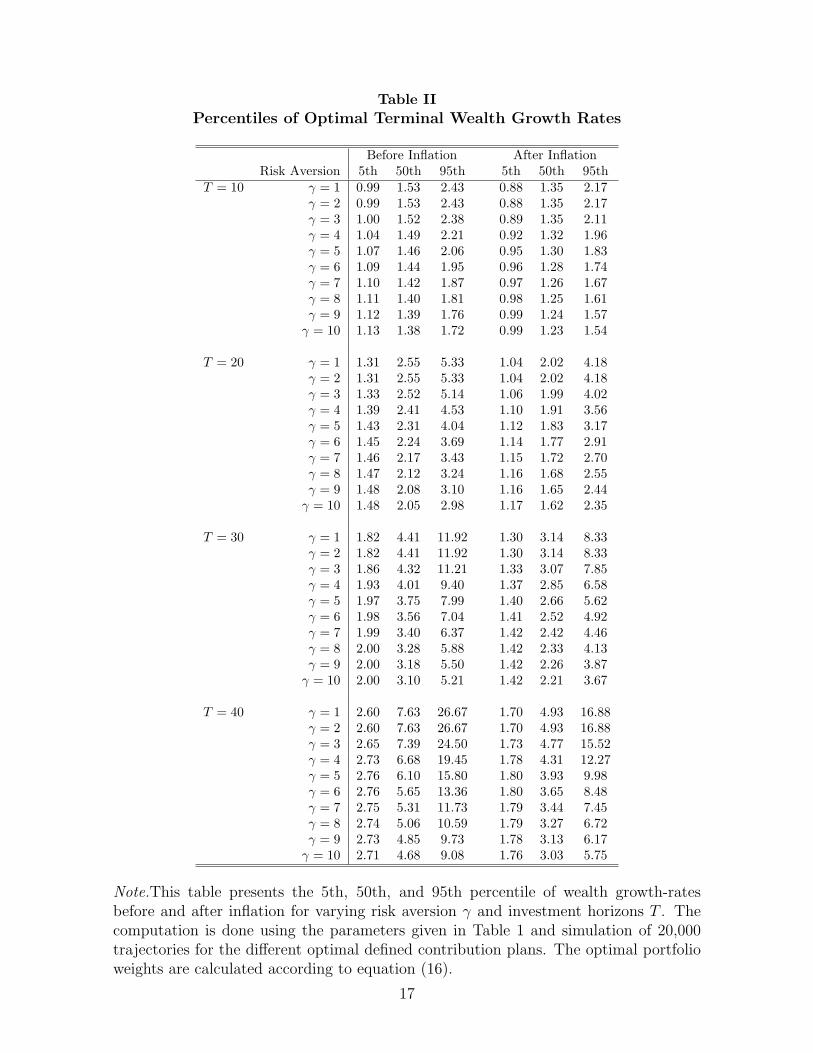
Table IIPercentiles of Optimal Terminal Wealth Growth Rates
Before Inflation After InflationRisk Aversion 5th 50th 95th 5th 50th 95th
T = 10 γ = 1 0.99 1.53 2.43 0.88 1.35 2.17γ = 2 0.99 1.53 2.43 0.88 1.35 2.17γ = 3 1.00 1.52 2.38 0.89 1.35 2.11γ = 4 1.04 1.49 2.21 0.92 1.32 1.96γ = 5 1.07 1.46 2.06 0.95 1.30 1.83γ = 6 1.09 1.44 1.95 0.96 1.28 1.74γ = 7 1.10 1.42 1.87 0.97 1.26 1.67γ = 8 1.11 1.40 1.81 0.98 1.25 1.61γ = 9 1.12 1.39 1.76 0.99 1.24 1.57
γ = 10 1.13 1.38 1.72 0.99 1.23 1.54
T = 20 γ = 1 1.31 2.55 5.33 1.04 2.02 4.18γ = 2 1.31 2.55 5.33 1.04 2.02 4.18γ = 3 1.33 2.52 5.14 1.06 1.99 4.02γ = 4 1.39 2.41 4.53 1.10 1.91 3.56γ = 5 1.43 2.31 4.04 1.12 1.83 3.17γ = 6 1.45 2.24 3.69 1.14 1.77 2.91γ = 7 1.46 2.17 3.43 1.15 1.72 2.70γ = 8 1.47 2.12 3.24 1.16 1.68 2.55γ = 9 1.48 2.08 3.10 1.16 1.65 2.44
γ = 10 1.48 2.05 2.98 1.17 1.62 2.35
T = 30 γ = 1 1.82 4.41 11.92 1.30 3.14 8.33γ = 2 1.82 4.41 11.92 1.30 3.14 8.33γ = 3 1.86 4.32 11.21 1.33 3.07 7.85γ = 4 1.93 4.01 9.40 1.37 2.85 6.58γ = 5 1.97 3.75 7.99 1.40 2.66 5.62γ = 6 1.98 3.56 7.04 1.41 2.52 4.92γ = 7 1.99 3.40 6.37 1.42 2.42 4.46γ = 8 2.00 3.28 5.88 1.42 2.33 4.13γ = 9 2.00 3.18 5.50 1.42 2.26 3.87
γ = 10 2.00 3.10 5.21 1.42 2.21 3.67
T = 40 γ = 1 2.60 7.63 26.67 1.70 4.93 16.88γ = 2 2.60 7.63 26.67 1.70 4.93 16.88γ = 3 2.65 7.39 24.50 1.73 4.77 15.52γ = 4 2.73 6.68 19.45 1.78 4.31 12.27γ = 5 2.76 6.10 15.80 1.80 3.93 9.98γ = 6 2.76 5.65 13.36 1.80 3.65 8.48γ = 7 2.75 5.31 11.73 1.79 3.44 7.45γ = 8 2.74 5.06 10.59 1.79 3.27 6.72γ = 9 2.73 4.85 9.73 1.78 3.13 6.17
γ = 10 2.71 4.68 9.08 1.76 3.03 5.75
Note.This table presents the 5th, 50th, and 95th percentile of wealth growth-ratesbefore and after inflation for varying risk aversion γ and investment horizons T . Thecomputation is done using the parameters given in Table 1 and simulation of 20,000trajectories for the different optimal defined contribution plans. The optimal portfolioweights are calculated according to equation (16).
17

of 1 for a 65 year old individual at time T is calculated actuarially fair according to
a(65, T ) =∞∑
s=0
p(65, s)(1 + δ)sP (T, s), (17)
where p(65, s) is the probability that the retiree survives to age 65 + s given that he
is alive at age 65 and (1 + δ) is the annual growthrate of annuity payments. Survival
probabilities are taken from the DAV 2004 Aggregate 1 mortality tables for females
with trend adjustment to account for mortality improvements. We set δ = 0.02 which
is approximately commensurate to expected inflation. This parameterization ensures
that the real income from annuities during retirement is flat in expectation. The con-
version of nominal terminal wealth W nT leads to an initial nominal annuity income of
W nT /a(65, T ). We divide this income by the last pre-retirement labor income in order
to calculate the so-called replacement ratio which is a commonly used measure to assess
which labor income drop the retiree can compensate.
The range of simulated replacement ratios for various risk aversions and investment
horizons appears in Table III. Together with the level of replacement ratios, the variabil-
ity of outcomes rises drastically over time. While the low risk strategy γ = 10 produces
outcomes which lie between 2.3 (5th percentile) and 4.17 percent (95th percentile) for
T = 10, corresponding values for T = 40 are 16.8 (5th percentile) and 65.9 percent
(95th percentile). The increase is amplified even further for the high risk strategy, so
that the replacement ratio at the 95th percentile is more than ten times higher than
the one at the 5th percentile (190.2 versus 16.1 percent). Since most private investors
do not now which γ they have, Table III is useful to assess how long and how risky
one should invest in order to attain a certain additional income during retirement with
a certain probability. The probable minimum replacement ratio (5th percentile) is an
important indicator if the investor needs a certain additional income with high confi-
dence. For instance, if the investor needs an additional pension income of 16 percent he
has to start accumulating at age 25 (i.e. T = 40). This will ensure that he reaches his
18

Table IIIPercentiles of Optimal Replacement Ratios
T = 10 T = 205th 50th 95th 5th 50th 95th
γ = 1 2.07 3.38 5.73 γ = 1 5.07 10.46 23.62γ = 2 2.07 3.38 5.73 γ = 2 5.07 10.46 23.62γ = 3 2.10 3.36 5.62 γ = 3 5.15 10.34 22.73γ = 4 2.17 3.29 5.23 γ = 4 5.34 9.91 20.05γ = 5 2.23 3.24 4.91 γ = 5 5.48 9.52 17.93γ = 6 2.26 3.19 4.68 γ = 6 5.56 9.19 16.43γ = 7 2.29 3.14 4.49 γ = 7 5.61 8.92 15.34γ = 8 2.31 3.11 4.36 γ = 8 5.64 8.71 14.53γ = 9 2.32 3.08 4.25 γ = 9 5.65 8.55 13.90γ = 10 2.33 3.06 4.17 γ = 10 5.66 8.41 13.41
T = 30 T = 405th 50th 95th 5th 50th 95th
γ = 1 9.58 24.72 71.78 γ = 1 16.21 50.77 190.20γ = 2 9.58 24.72 71.78 γ = 2 16.21 50.77 190.20γ = 3 9.77 24.20 67.81 γ = 3 16.52 49.19 176.17γ = 4 10.11 22.47 56.56 γ = 4 17.08 44.38 140.12γ = 5 10.31 21.02 48.29 γ = 5 17.25 40.50 114.28γ = 6 10.40 19.88 42.56 γ = 6 17.25 37.59 96.54γ = 7 10.41 19.04 38.53 γ = 7 17.19 35.48 84.94γ = 8 10.42 18.37 35.68 γ = 8 17.09 33.75 76.75γ = 9 10.40 17.83 33.45 γ = 9 16.97 32.32 70.60γ = 10 10.37 17.38 31.73 γ = 10 16.82 31.18 65.93
Note.This table presents the 5th, 50th, and 95th percentile of replacement ratios forvarious risk aversions γ and investment horizons T . The replacement ratio is defined asthe first annuity income divided by the last pre-retirement labor income whereby it isassumed that the terminal wealth is converted into a life-long escalating annuity. Thecomputation is done using the parameters given in Table 1 and simulation of 20,000trajectories for the different optimal defined contribution plans. The optimal portfolioweights are calculated according to equation (16).
goal with approximately 95 percent probability. On the other hand, an investor which
already has a high and secure pension income from other sources (e.g. public pension or
defined benefit plans) might not need to save as long and prefer a more risky strategy.
4.2 Utility Costs of Suboptimal Strategies
This section is devoted to the evaluation of the most common asset allocation schemes
for defined contribution plans against the optimal strategy derived above. To this end,
19

we consider the following asset five allocation schemes:
1. Pure stock/bond/money plans. Although those strategies do not gain from
diversification among asset classes we introduce them in order to gain insight into the
long term risk and return profile implied by the assumed model and parameterization
of the three asset classes stocks, bonds, and money. Especially pure money plans are
the most often default option offered in defined contribution plans if participants do
not actively change the investment option (Holden and Venderhei, 2005).
2. Constant mix strategies. In the class of constant mix strategies we consider the
60/40 stock bond mix. The upside of constant mix strategies is that they are easy
to realize for the provider from an administration perspective if there already exists a
mutual fund for each asset class.
3. Life-cycle strategies. We implement the strategy commonly known as the
”100−minus−age” strategy which invests 100− age percent in stocks and the remainder
in bonds.
4. Static portfolio insurance. The common notion of portfolio insurance strategies
is restrict the downside risk at the end of the pension plan. The usual guarantee is that
at the end of the pension plan at least the sum of invested contributions is attained.
We construct the strategy such that always as many zero coupon bonds as needed
to maintain a nominal return guarantee are held in the portfolio. The part which is
invested into zero bonds is exactly the present value of the money-back guarantee of the
nominal contribution. Here the zero bonds have the same duration as the remaining
pension plan maturity. This strategy is basically a cash-flow matching strategy and has
the advantage that the minimum return guarantee is met with 100 percent probability.
5. Dynamic portfolio insurance. These portfolio insurance strategies dynamically
control the stock fraction over time, usually such that at the end of the pension plan
the value of the portfolio exceeds the sum of contributions (in nominal terms). We
employ the famous constant proportion portfolio insurance strategy (CPPI) in which
20

the stock fraction is set according to:
πSt = min
(m
F nt −Bt
F nt
, 1
), (18)
where m is the so-called multiplier and Bt is the present value of the sum of contributions
made until t. We set the multiplier to 4. Since we assume that the portfolio is balanced
monthly, setting the multiplier to 4 implies that the assumed maximal loss of stock
markets in one month is 1/4 = 25 percent. The bond fraction is set to 1 − πSt . The
motivation of this strategy is that in contrast to static portfolio insurance a certain
probability to miss the nominal return guarantee is tolerated in order to increase the
expected return. This, because static portfolio insurance strategies have to start from
the beginning with a certain bond fraction in order to keep the money-back guarantee,
the CPPI strategy starts out with a pure stock portfolio and switches to bonds only if
the money-back guarantee is jeopardized. Hence, the risk and return profiles of both
portfolio insurance strategies are fundamentally different, except for the fact that both
have the goal to keep the money-back guarantee at the end of the investment horizon.
We assess the risk and return efficiency of the described strategies in terms of
utility losses relative to the optimum. To this end, we calculate the certainty equivalent
wealth for each considered strategy and compare it to that of the optimal strategy. The
certainty equivalent wealth (CEW) denotes the riskless terminal wealth in real terms
which the individual needs to be indifferent between following a certain asset allocation
strategy and earning the CEW. Formally, the CEW is defined by the condition
u(CEW ) = E[u(W rT )] (19)
Having calculated the CEW levels for the optimal strategies and the practicable in-
vestment plans we compute the relative difference between the CEW of the practicable
strategies and that of the optimal strategy. Since the evaluation of the strategy heavily
21

T=20
0
5
10
15
20
25
30
35
40
45
50
1 2 3 4 5 6 7 8 9 10RRA
Util
ity L
oss
in C
EW
Ter
ms
(Per
cent
)
Stocks Dynamic Portfolio Insurance60/40 Stocks/Bonds LifecycleStatic Portfolio Insurance BondsMoney
T=40
0
10
20
30
40
50
60
70
1 2 3 4 5 6 7 8 9 10RRA
Util
ity L
oss
in C
EW
Ter
ms
(Per
cent
)
Stocks Dynamic Portfolio Insurance60/40 Stocks/Bonds Life-Cycle (100-age)Static Portfolio Insurance BondsMoney
Figure 4: Relative Loss in Certainty Equivalent Wealth of Practicable Strategies Com-pared to the Optimum. This figure shows for various degrees of risk aversions the utilityloss of following a suboptimal strategy compared to the optimal strategy. The calcu-lation is done via Monte Carlo simulations (20,000 paths) for a defined contributionplans with the duration of T = 20 (upper graph) and T = 40 years (lower graph).
depends on the risk aversion parameter we calculate the relative loss in CEW for a
range of risk aversions between γ = 1 and γ = 10.
The results of this analysis are reported in Figure (4) for the investment horizons
T = 20 and T = 40. Conveniently, we identify three segments of risk aversion (low,
moderate, and high). The upper graph displays the results for T = 20. At very low
22

degrees of risk aversion around γ = 1 and γ = 2 investors would prefer stock based
investments like the pure stock plan and the dynamic portfolio insurance so that utility
losses of that strategies are quite small. Utility losses of diversified strategies which mix
asset classes like the constant mix, life-cycle, static portfolio insurance strategy would
be around 20 percent. Holding a pure bond or money plan would lead to significant
utility losses of around 40 percent. For moderate risk aversions in the range γ = 3 to
γ = 8 the 100-minus-age rule and the constand mix strategy are closest to the opti-
mum with utility losses below 10 percent. The stock based strategies lead already to
high utility discounts up to 20 percent while the bond based strategy leads to losses
of about 15 to 30 percent. The pure money market investment leads to high losses of
more than 30 percent. For high risk aversions γ = 9 to γ = 10 the static portfolio
insurance together with the 100-minus-age rule and the constand mix strategy become
the preferred strategies with utility losses below 5 percent. In this high risk aversion
segment stock based strategies lead to utility losses of around 25 percent, and similar
results are obtained for pure money market plans. It is also noteworthy that the dy-
namic portfolio insurance and static portfolio insurance strategy exhibit fundamentally
different risk profiles although both have the main goal to warrant the nominal money-
back guarantee. By and large, the pattern of results stays the same for T = 40 (lower
graph), except for that utility losses increase by about 20 percent for all strategies.
The analysis reveals that utility losses can be extremely high if investors choose a
strategy which does not reflect their risk aversion. Utility losses can be especially high if
the portfolio is underdiversified and only one asset class is held. Conversely, strategies
which mix asset classes benefit from having a more moderate risk-return profile. In
turn, if investors do not know their risk aversion exactly, diversified strategies should
be preferred. They are most attractive to moderately risk averse investors and lead to
small utility losses at the ends of the risk aversion spectrum. This result makes clear
how crucial the estimation of the investor attitude towards risk is, particularly if the
23

investment horizon is so long. Investment risks have to be clarified to the investor so
that he can choose the most suitable portfolio strategy. Furthermore, the risk aversion
parameter should reflect background risks of the individual, which can hardly been
modeled explicitly. For instance, it might be necessary to adjust the risk aversion
parameter in order to take into account other components of household wealth such as
human capital, housing, and insurance wealth.
5 Conclusions
In the light of the disillusioning evidence on household financial literacy, the present
paper has derived relatively simple optimal asset allocation rules which could serve
as default options for defined contribution plans. To be practicable for pension plan
providers we impose short selling restrictions and require the optimal asset allocation
strategy to evolve deterministically over time rather than stochastically. From the
view of plan participants this deterministic life-cycle strategy is transparent and easily
comprehensible since they ex-ante know which asset allocation will be held at future
dates. Further, performance losses due to administration as well as transactions costs
can be avoided. Thereby, our assumed asset model accounts for the major long-term
investment risks: stock market price risk, expected and unexpected inflation risk as
well as interest rate risk.
Regarding the optimal asset allocation our results conform to recent studies in-
cluding non-financial income inasmuch the equity fraction declines until the retirement
phase is reached. The reason is that the present value of future contributions is per-
ceived as a bond investment so that it is optimal to engage higher stock fractions in
the beginning of the pension plan and to decrease the fraction commensurately to the
decline in the present value of future contributions. The higher the risk aversion the
faster declines the stock fraction.
24

Our Monte Carlo analysis shows that the choice of the asset accumulation strategy
and the length of the investment horizon have significant impact on the outcome of the
accumulation plan and hence standard of living during retirement. Investors should
definitely be aware of how long they should accumulate retirement wealth and how
risky they should invest in order to achieve the appropriate dispersion of retirement
wealth or annuity income if wealth is converted into a life-annuity.
Our final welfare analysis suggests that typical asset allocation schemes found in
practice are close to the optimum in terms of certainty equivalent wealth comparisons if
the scheme is chosen commensurately to the risk appetite of the plan participant so that
utility losses are around 5 percent if the risk aversion of the participant is estimated
correctly. However, if an asset allocation strategy is chosen that does no reflect the risk
aversion of the investor, utility losses can reach up to 60 percent. Utility losses become
particularly severe for longer investment horizons.
25

References
Babbs, S., and K. Nowman, 1999, “Kalman Filtering of Generalized Vasicek-Term
Structure Models,” The Journal of Financial and Quantitative Analysis, 34 (1), 115–
130.
Barber, B., and T. Odean, 2000, “Trading Is Hazardous to Your Wealth: The Common
Stock Investment Performance of Individual Investors,” Journal of Finance, 55 (2),
773–806.
Beshears, J., J. Choi, D. Laibson, and B. Madrian, 2006, “The Importance of De-
fault Options for Retirement Saving Outcomes: Evidence from the United States,”
Discussion paper, NBER, No. 12009.
Brandt, M., 1999, “Estimating Portfolio and Consumption Choice: A Conditional Euler
Equations Approach,” Journal of Finance, 54, 1609–1645.
Brennan, M., and Y. Xia, 2000, “Stochastic Interest Rates and Bond-Stock Mix,”
European Finance Review, 4, 197–210.
Brennan, M., and Y. Xia, 2002, “Dynamic Asset Allocation under Inflation,” Journal
of Finance, 57, 1201–1238.
Cairns, A., D. Blake, and K. Dowd, 2006, “Stochastic Lifestyling: Optimal Dynamic
Asset Allocation for Defined-Contribution Pension Plans,” Journal of Economic Dy-
namics and Control, 30, 843–877.
Campbell, J., Y. Chan, and L. Viceira, 2003, “A Multivariate Model of Strategic Asset
Allocation,” Journal of Financial Economics, 67, 41–80.
Campbell, J., and L. Viceira, 1999, “Consumption and Portfolio Decisions When Ex-
pected Returns are Time-Varying,” Quarterly Journal of Economics, 114, 433–495.
26

Campbell, J., and L. Viceira, 2001, “Who Should Buy Long-Term Bonds,” The Amer-
ican Economic Review, 91, 99–127.
Carhart, M., 1997, “On persistence in mutual fund performance,” Journal of Finance,
52, 57–82.
Cocco, J., F. Gomes, and P. Maenhout, 2005, “Consumption and Portfolio Choice over
the Life Cycle,” The Review of Financial Studies, 18, 491–533.
Fitzenberger, B., R. Hujer, T. MaCurdy, and R. Schnabel, 2001, “Testing for uniform
wage trends in West-Germany: A cohort analysis using quantile regressions for cen-
sored data,” Empirical Economics, 112, 41–86.
Holden, S., and J. Venderhei, 2005, “401(k) Plan Asset Allocation, Account Balances,
and Loan Activity in 2004,” Discussion paper, EBRI Issue Brief, No. 285, Investment
Company Institute and Temple University.
Huberman, G., S. Iyengar, and W. Jiang, 2007, “Defined Contribution Pension Plans:
Determinants of Participation and Contributions Rates,” Journal of Financial Ser-
vices Research, 31, 1–32.
Iyengar, S., and M. Lepper, 2000, “When Choice is Demotivating: Can One Desire
Too Much of a Good Thing?,” Journal of Personality and Social Psychology, 79,
995–1006.
Merton, R., 1969, “Lifetime Portfolio Selection under Uncertainty: The Continous Time
Case,” Review of Economics and Statistics, 51 (3), 239–246.
Merton, R., 1971, “Optimum Consumption and Portfolio Rules in a Continuous-Time
Model,” Journal of Economic Theory, 3 (4), 373–413.
Munk, C., C. Soerensen, and T. Vinther, 2004, “Dynamic asset allocation under mean-
reverting returns, stochastic interest rates, and inflation uncertainty: Are popular
27

recommendations consistent with rational behavior?,” International Review of Eco-
nomics & Finance, 13, 141–166.
Poterba, J., J. Rauh, S. Venti, and D. Wise, 2005, “Lifecycle Asset Allocation Strategies
and the Distribution of 401(k) Retirement Wealth,” Discussion paper, NBER, No.
11974.
Shafir, E., I. Simonson, and A. Tversky, 1993, “Reason-based Choice,” Cognition, 49,
11–36.
Shiller, R., 2005, “The Life-Cycle Personal Accounts Proposal for Social Security: An
Evaluation,” Discussion paper, Yale University.
Tversky, A., and E. Shafir, 1992, “”Choice Under Conflict: The Dynamics of Deferred
Decision,” Psychological Science, 3, 358–361.
van Rooij, M., C. Kool, and H. Prast, 2007, “Risk return preferences in the pension
domain: are people able to choose?,” Journal of Public Economics, 91, 701–722.
Vasicek, O., 1977, “An Equilibrium Characterization of the Term Structure,” Journal
of Financial Economics, 5, 177–188.
Viceira, L., 2007, “Life-Cycle Funds,” Discussion paper, Harvard Business School.
Wachter, J., 2002, “Portfolio and Consumption Decisions Under Mean-Reverting Re-
turns: An Exact Solution for Complete Markets,” Journal of Financial and Quanti-
tative Analysis, 37, 63–91.
Wachter, J., 2003, “Risk Aversion and Allocation to Long-Term Bonds,” Journal of
Economic Theory, 112, 325–333.
28