Optimal Lag Structure Selection inVEC–Models∗

Peter Winker† Dietmar Maringer‡

Preliminary version: February 26, 2004

Abstract

For the modelling of economic and financial time series, multivari-ate linear and nonlinear systems of equations became a standard tool.These models might also be applied in the context of non–stationaryprocesses. However, estimation results in finite samples might dependstrongly on the specification of the model dynamics.

We propose a method for automatic identification of the dynamicpart of VEC–models. Model selection is based on a modified infor-mation criterion. The lag structure of the model is selected accordingto this objective function allowing for “holes”. The resulting com-plex discrete optimization problem is tackled using a hybrid heuristiccombining ideas from threshold accepting and memetic algorithms.We present the algorithm and results of a simulation study indicat-ing the performance both with regard to the dynamic structure andthe rank selection in the VEC–model. The results indicate that theselected rank might depend strongly on the dynamic specification ofthe VEC–model.

Keywords: Model selection; cointegration rank; information criterion; orderselection; reduced rank regression; VECM.JEL classification: C32; C61.

∗We are indebted to D. Hendry, S. Johanson, K. Juselius, H. Lutkepohl and M. Meyerfor helpful comments on an earlier draft of this paper. All remaining shortcomings liesolely with the authors.†Department of Economics, Law and Social Sciences, University of Erfurt‡Department of Economics, Law and Social Sciences, University of Erfurt

1

1 Introduction

For the modelling of economic and financial time series, multivariate linear(VAR, SVAR, VECM) and nonlinear systems of equations (MS–VAR) be-came a standard tool over the last few years. As compared to univariateapproaches, these models exhibit interesting features, e.g. dealing with non–stationary processes and cointegration. However, the issue of finite sampleperformance becomes even more relevant for these models which typicallyrequire the simultaneous estimation of a large set of parameters.1 Whileeconomic theory might provide a guideline for long–run or equilibrium rela-tionships,2 the modelling of the dynamic part has to rely on different inputs.3

In order to avoid a simple ad hoc specification of the dynamic part, severalstatistical procedures have been proposed. For example, the lag structure inVAR–models is based on tests on residual autocorrelation (Jacobson, 1995)or information criteria like AIC and BIC (Winker, 2000).4 However, theseapproaches did not take into account potential non–stationarity of the timeseries and the restrictions imposed by the rank conditions in a cointegrationframework. In several contributions,5 the effect of lag length selection on theoutcomes of tests for cointegration,6 in particular on the cointegration rank,has been demonstrated. Bewley and Yang (1998) compare the performanceof different system tests for cointegration when the lag length is selected bymeans of a standard information criterion (AIC or BIC, respectively). Bothunder– and overspecification of the lag length appear to have a negative im-pact.7 While the effect on size is small for tests for rank equal to zero, the

1For example, a small sample correction of Johansen’s test is proposed by Johansen(2002).

2The issue of identification and restriction of long–run relationships based on statisticaltests and prior information is discussed by Omtzigt (2002).

3In this paper, we neglect the specification of deterministic trend terms, which mighthave similar implications on the outcomes (Ahking, 2002).

4A different approach focusing on general–to–specific reductions, which eliminates sta-tistically insignificant variables and uses diagnostic tests to check the validity of reductionsis presented by Hendry and Krolzig (2001) and Krolzig and Hendry (2001). Bruggemannet al. (2003) provide a comparison of different methods.

5See also the references provided by Ho and Sørensen (1996) in their introduction andby Potscher (1991).

6In general, the analysis is conducted in the framework of Johansen’s testing procedure(Johansen, 1988; Johansen, 1991; Johansen, 1992; Johansen, 1995).

7Gonzalo and Pitarakis (1999) analyse the performance of model selection criteria inlarge dimensional VARs. They find that underfitting might become as important as over-

2

effect on power is more substantial for certain parameter combinations. Thiseffect becomes even more pronounced for tests of the null of a cointegrationrank of one. Ho and Sørensen (1996) considered higher dimensional systemsand found that the negative impact of overspecification increases with the di-mension. In particular, application of Johansen’s test tends to underestimatethe number of unit roots in the system, and, in due course, to overestimatethe cointegration rank in this case.

The model selection procedure analyzed in this paper differs in two as-pects from the methods mentioned above. First, we employ a modified in-formation criterion discussed by Chao and Phillips (1999) for the case ofpartially nonstationary VAR–models.8 Consequently, the dynamic model se-lection is performed taking the restrictions of reduced rank regressions intoaccount. Second, we allow for “holes” in the lag structures, i.e. lag structuresare not constrained to sequences of lags up to lag k, but might consist, e.g.,of the first and fourth lag only in an application to quarterly data. Using thisapproach, different lag structures can be used for different variables and indifferent equations of the system. This feature has to be taken into account inthe estimation procedure for a given dynamic structure.9 For this purpose,we use a SURE–like modification of the two step reduced rank estimatorproposed by Ahn and Reinsel (1990).10

Using this approach, the problem of model specification becomes an inte-ger optimization problem on the huge set of all possible lag structures. In thecontext of VAR–models several methods have been proposed to tackle thisproblem of high computational complexity. Exact algorithms are based on anintelligent enumeration of possible models avoiding the evaluation of all cases

fitting when the dimension of the process increases even for the AIC. Furthermore, theperformance of information criteria depends critically on the specific DGP under consid-eration.

8Analyzing the effects of choosing alternative criteria, e.g. along the lines suggested byCampos et al. (2003), is left for future research. The same applies to the combination witha pre–selecting step also discussed by Campos et al. (2003).

9As pointed out by Gredenhoff and Karlsson (1999), in the literature on model selectionin VAR–models, the possibility that the true model may have unequal lag–length or evenholes in the lag structure has received little attention. Although they use the Hsiaoprocedure which does not investigate all combinations of lag–lengths for the differentvariables and does not allow for holes at all, their simulation results indicate that, inparticular for more complex lag structures, their unequal lag length procedure appearsimprove results.

10An application in the ML setting of Johansen’s procedure is left for future research.

3

(Gatu and Kontoghiorghes, 2003). Nevertheless, this approach is still of highcomputational complexity and appears to be limited in the current stage tolinear models without further restrictions. In contrast, heuristic optimizationtechniques which have already been applied to the linear VAR (Winker, 2000)can be extended to structural VAR– and VEC–models. However, the numer-ical methods used in estimating the model for a given dynamic structure, i.e.the two step reduced rank estimator used in this paper or a ML estimator,become more involved in a VEC setting. In due course, the overall computa-tional complexity increases. This high computational load sets a limit to thenumber of different data generating processes (DGP) and parameter settingswhich can be used for our MC simulation analysis. Nevertheless, our firstresults indicate that the method works well in practice and might be superiorto the standard “take all up to the k–th lag” approach in specific settings.

The paper is organized as follows. Section 2 introduces the model se-lection problem in the context of VEC–models. We present the model, theinformation criteria and the resulting integer optimization problem. Section 3describes the implementation of the heuristic used to solve this optimizationproblem. In section 4 we present some Monte Carlo evidence on the per-formance of the method applied to different data generating processes. Theresults are compared to the standard method of choosing all lags up to acertain order. Section 5 summarizes the findings and provides an outlook tofurther steps of our analysis.

2 The Model Selection Procedure

The standard procedure for model selection in a VEC–model setting consistsof a sequential procedure. First, information criteria like AIC or BIC areused to choose a lag length for the unrestricted VAR–model.11 For the nextsteps of the analysis, it is assumed that the correct specification of the lagstructure is given.12 Then, for the determination of the cointegration rank,a sequence of cointegration tests is performed. The statistical properties of

11Ho and Sørensen (1996) find evidence in favour of using BIC when a cointegrationanalysis is intended. Winker (1995, 2000) generalizes this model selection step to allowfor different lag structures across equations including “holes”.

12However, several simulation studies have demonstrated that lag misspecification ad-versely affects the outcome of the cointegration tests conducted in the second step (Hoand Sørensen, 1996; Bewley and Yang, 1998).

4

this sequential procedure are difficult to assess. Consequently, it cannot beguaranteed that the final estimation of the cointegration rank obtained bythis procedure is a consistent estimate (Johansen, 1992; Jacobson, 1995; Chaoand Phillips, 1999).

In order to circumvent these shortcomings of the traditional approach,Chao and Phillips (1999) propose to reconsider the problem from the view-point of model selection.13 They propose a modification of the BIC and aposterior information criterion (PIC) for the application to VAR processeswith reduced rank cointegration structure. Using these criteria for model se-lection exhibits three advantages: First, lag structure and the cointegrationrank can be selected in a single step. Second, the penalty function of bothcriteria reacts to under– and over–parameterization, which both might havea detrimental effect on the estimation of the cointegration rank (Bewley andYang, 1998). Application of this criterion provides a consistent estimation oflag structure and cointegration rank (Chao and Phillips, 1999). Third, themethod can easily be extended to cover the case of different lag structuresacross equations including “holes”.

For the MC simulations presented in this paper, we consider both themodified BIC (BICm) and the modified posterior information criterion (PICm)presented in Chao and Phillips (1999, p. 236). However, the PICm is consid-ered solely for a comparison of different criteria applied to models containingall lags up to a certain order. Our goal is to assess the advantage of allowingfor holes in the lag structure for the determination of the cointegration rankof a VECM as compared to the standard “take all up to the k–th lag” ap-proach. For the optimization of lag structures allowing for holes, we restrictthe analysis to the BICm for computational reasons. Inclusion of the PICmis part of our future research agenda.

We consider the d–dimensional VAR–model of order k + 1

Yt =k+1∑i=1

ΠiYt−i + εt (1)

with initial values Y0, Y−1, ..., Y−k. Thereby, the error terms εt are assumedto be iid N (0,Ω). Furthermore, it is assumed that the characteristic poly-nomial of the VAR may have unit roots on the unit circle, but no explosive

13Bahmani-Oskooee and Brooks (2003) also propose a global criterion based on thegoodness of fit of the resulting long–run relationships. However, they do not provide MCevidence on the relative performance of this approach.

5

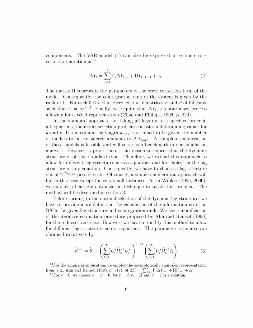
components. The VAR–model (1) can also be expressed in vector error–correction notation as14

∆Yt =k∑i=1

Γi∆Yt−i + ΠYt−k−1 + εt . (2)

The matrix Π represents the parameters of the error correction term of themodel. Consequently, the cointegration rank of the system is given by therank of Π. For each 0 ≤ r ≤ d, there exist d · r matrices α and β of full ranksuch that Π = αβ′.15 Finally, we require that ∆Yt is a stationary processallowing for a Wold representation (Chao and Phillips, 1999, p. 229).

In the standard approach, i.e. taking all lags up to a specified order inall equations, the model selection problem consists in determining values fork and r. If a maximum lag length kmax is assumed to be given, the numberof models to be considered amounts to d ·kmax. A complete enumerationof these models is feasible and will serve as a benchmark in our simulationanalysis. However, a priori there is no reason to expect that the dynamicstructure is of this standard type. Therefore, we extend this approach toallow for different lag structures across equations and for “holes” in the lagstructure of any equation. Consequently, we have to choose a lag structureout of 2d

2·kmax possible sets. Obviously, a simple enumeration approach willfail in this case except for very small instances. As in Winker (1995, 2000),we employ a heuristic optimization technique to tackle this problem. Themethod will be described in section 3.

Before turning to the optimal selection of the dynamic lag structure, wehave to provide more details on the calculation of the information criterionBICm for given lag structure and cointegration rank. We use a modificationof the iterative estimation procedure proposed by Ahn and Reinsel (1990)for the reduced rank case. However, we have to modify this method to allowfor different lag structures across equations. The parameter estimates areobtained iteratively by

bι+1 = bι +

(T∑t=1

U∗t Ω−1ε U∗

′t

)(−1)( T∑t=1

U∗t Ω−1ε εt

)(3)

14For the empirical application, we employ the asymptotically equivalent representationfrom, e.g., Ahn and Reinsel (1990, p. 817), of ∆Yt =

∑ki=1 Γi∆Yt−i + ΠYt−1 + εt.

15For r = 0, we choose α = β = 0, for r = d, α = Π and β = I is a solution.

6

where ι is the current iteration, Ωε is the covariance matrix of the residuals,ε, under the current parameter estimates βι and

U∗t =[(α′ ⊗ [0, Id−r]Yt−1)′, Id ⊗ [(βYt−1)′,∆Yt−1, ...,∆Yt−k]

′]′(4)

where β is normalized so that β = [Ir, β0]. The matrices Π and Γi can thenbe determined by decomposing the parameter vector b with

b = [vec(β′0)′, vec((α,Γ1, ...,Γk)′)′]′ . (5)

The initial solution for b0, can be found from a full rank SUR estimatewhich decreases the number of necessary iterations significantly and thereforeincreases the convergence speed.

To introduce the “holes” into the lag structure, i.e., setting some of theelements of the Γi’s equal to 0, the respective columns in U∗

′t are eliminated

and the (de–)composition of b has to be adapted. The information criterionBICm can then be calculated according to

BICm = ln |ΩΥ,r|+ ν + r(d− r) + dr

T· ln(T ) (6)

where Υ denotes the set of elements of the Γi’s, and ν = ]Υ, i.e. is thenumber of elements of the Γi’s that are not equal to zero. ΩΥ,r is computedfollowing Chao and Phillips (1999) in two steps: first, the parameters α,β and Γi are estimated iteratively as described previously for given rank rand lag structure Υ. Next, the corrected values ∆Y ∗t = ∆Yt − αβ′Yt−1 arecomputed. Finally, the Γi’s are re–estimated by running a SUR estimationof ∆Y ∗t on the ∆Yt−i’s included in the given lag structure Υ. ΩΥ,r denotesthe covariance matrix of the residuals of this last regression.

3 The Algorithm

The algorithm for finding the optimal lag structure allowing for holes is ahybrid heuristic combining ideas of the Threshold Accepting (TA) algorithmas described in Winker (2001) and of “Memetic Algorithms”16. For a givencointegration rank r, a random initial lag structure is chosen, the parametersare estimated and the value for the information criterion BICm is computed

16Cf. Moscato (1999) and Maringer and Winker (2003).

7

along the lines described in the previous section. During the following itera-tion steps, a local search strategy is employed where the structure is modifiedby either including one additional or excluding one hitherto included laggedvariable in one of the equations. If the information criterion is improved orif the impairment is acceptable in the sense that it does not exceed a giventhreshold, i.e. if ∆BICm ≤ Ti, the modified lag structure is accepted. If,however, the modified lag structure degrades the information criterion morethan tolerated by the current value of the threshold sequence, this modi-fication is undone and the previous lag structure is restored. During theearly iteration steps, the threshold is chosen rather generously and most ofthe modifications are actually accepted. In the course of the iterations, thethreshold is persistently lowered, so that hardly any impairment is acceptedin the last iterations. Consequently, the algorithm is well apt to overcomelocal optima and to fine–tune the solution once the “core structure” has beenidentified.

Whereas in TA a single agent is representing one solution per iteration, weenhanced the original TA concept much in the sense of Memetic Algorithmsby replacing the single agent by a population of agents each of which followsthe TA search strategy. In addition to their independent local search, theagents “compete” with each other on a regular basis where one agent chal-lenges another and passes his (current) structure on to the challenged agentif the change in the challenged agent’s information criterion does not violatethe threshold criterion. Also, agents can combine parts of their solutionsusing a cross–over operator (Fogel, 2001) where an offspring will replace aparent if, again, the impairment in the information criterion does not exceedthe threshold.

The heuristic optimization is repeated for all possible values of the rankr, i.e. 0 ≤ r ≤ d − 1.17 Let BICmr denote the minimum value of theinformation criterion obtained by the optimization heuristic for a rank of r.Let ropt = argmin0≤r≤d−1BICmr, then the finally selected model is the onewith rank ropt and the corresponding dynamic lag structure. The selection ofrank and lag length for the standard “take all up to the k–th lag” approachis performed in a similar way. For all possible values of the rank r and all k,0 ≤ k ≤ kmax, the value of the criterion BICm is calculated. The pair (r, k)

17The case r = d is not considered as it corresponds to a stationary VAR–model. Amethod for model selection in VAR–models by means of optimization heuristics is pre-sented in Winker (2000).

8

resulting in the minimum value of BICm describes the model identified bythe “take all up to the k–th lag” approach.18

4 Monte Carlo Simulation

4.1 Motivation

The evaluation of the information criterion BICm used for model selection inthis paper requires the estimation of the parameters of the reduced rank mod-els. For this purpose we employ the iterative algorithm proposed by Ahn andReinsel (1990). This procedure is quite time consuming even if good startingvalues are provided. Consequently, the number of iterations of our hybridheuristic has to be limited in order to allow for at least some replications in aMC setting. Finally, this high overall computational complexity of automaticlag order selection in the VEC–models limits the number of different settingswhich can be analyzed by means of MC simulation. Consequently, we triedto assess the relative performance of the method by considering a few typicalcases. Besides using artificial DGPs, we follow Ho and Sørensen (1996) forsome of our simulations by using parameter values obtained from an esti-mation using actual data. Given that our simulations can only pick a smallnumber of parameter settings out of a huge parameter space, this approachascertains that we might select empirically relevant parameter settings.

4.2 Simulation Setup

The results presented in this section are based on the simulation of threedifferent DGPs with different rank and lag structure. The details of theseDGPs are introduced below. The first DGP (DGP1) is taken from Chaoand Phillips (1999, pp. 242f, Experiment5). The second DGP (DGP2) isbased on this example, but adds a second cointegration vector and extendsthe dynamic structure. Finally, the third DGP (DGP3) is based on theestimation of a simple money demand system.

For each replication of the first two DGPs 300 observations have beengenerated from which the first 145 are eliminated, leaving a sample length

18Depending on the assumed rank r, the complexity of the lag structure and the lengthof the data series, the CPU time ranged from 3 to 7 minutes per independent optimizationrun on a Pentium 4 with 2.8 GHz using Matlab R13.

9

of T = 155. For DGP3, the process was initialized with the historical valuesof the variables and samples of length T = 200 have been simulated foreach replication. We ran 100 and 200 replications, respectively, and for eachreplication the rank was estimated by the methods “all up to the k-th lag”(labelled “all”) and our optimization heuristic allowing for structures with“holes” in the kmax lags (labelled “holes”) with kmax = 5 for both methods.

DGP1

Experiment 5 in Chao and Phillips (1999) is a three dimensional VECM withone cointegration vector entering a single equation of the system and a laglength of one. Thereby, lagged differences of the endogenous variables enteronly the equation for the respective variables. The error correction termis described by the matrix Π, Γ1 provides the coefficients of the dynamicpart and Ωε the variance–covariance matrix of the normally distributed errorterms:

Π =

0−0.01

0

(1 0.25 0.8

)

Γ1 =

0.99 0 00 0.9025 00 0 0.99

Ωε =

2.25 2.55 1.952.55 3.25 2.811.95 2.81 2.78

The modulus of nonzero reverse characteristic roots of the process19 are1, 1, 0.99, 0.99, 0.95, 0.95.

DGP2

Modifying the above DGP by adding a second cointegration vector and lagsof order 2 and 3 in the dynamic part, we obtain DGP2 with an actual rank

19See Lutkepohl (1993) for a description. The roots are calculated using a Maple im-plementation with 100 digit precision.

10

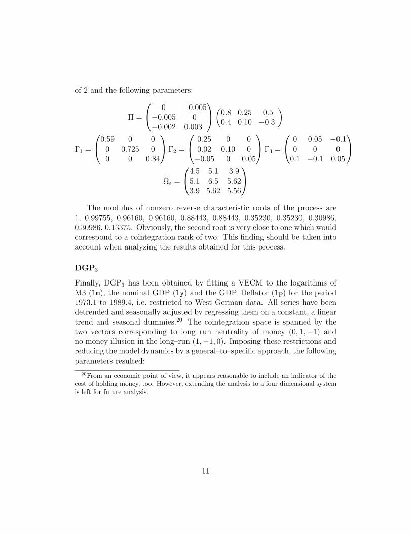
of 2 and the following parameters:

Π =

0 −0.005−0.005 0−0.002 0.003

(

0.8 0.25 0.50.4 0.10 −0.3

)

Γ1 =

0.59 0 00 0.725 00 0 0.84

Γ2 =

0.25 0 00.02 0.10 0−0.05 0 0.05

Γ3 =

0 0.05 −0.10 0 0

0.1 −0.1 0.05

Ωε =

4.5 5.1 3.95.1 6.5 5.623.9 5.62 5.56

The modulus of nonzero reverse characteristic roots of the process are1, 0.99755, 0.96160, 0.96160, 0.88443, 0.88443, 0.35230, 0.35230, 0.30986,0.30986, 0.13375. Obviously, the second root is very close to one which wouldcorrespond to a cointegration rank of two. This finding should be taken intoaccount when analyzing the results obtained for this process.

DGP3

Finally, DGP3 has been obtained by fitting a VECM to the logarithms ofM3 (lm), the nominal GDP (ly) and the GDP–Deflator (lp) for the period1973.1 to 1989.4, i.e. restricted to West German data. All series have beendetrended and seasonally adjusted by regressing them on a constant, a lineartrend and seasonal dummies.20 The cointegration space is spanned by thetwo vectors corresponding to long–run neutrality of money (0, 1,−1) andno money illusion in the long–run (1,−1, 0). Imposing these restrictions andreducing the model dynamics by a general–to–specific approach, the followingparameters resulted:

20From an economic point of view, it appears reasonable to include an indicator of thecost of holding money, too. However, extending the analysis to a four dimensional systemis left for future analysis.

11

ΠYt−1 =

0 00.20237 −0.20453−0.069713 0.16597

(

1 −1 01 0 −1

)

lmt−1

lyt−1

lpt−1

Γ1 =

0 0 00 −0.35885 −0.558450 0 0.29401

Γ2 =

0 0 0.285110.42088 −0.24879 −0.28601

0 0 0

Γ3 =

0.15953 0 00.38674 0 −0.326080.026677 0 0

Γ4 =

0.13814 −0.087458 −0.208020.19475 0.24129 0

0 −0.090326 0.062985

Γ5 =

0 0 0.207210 0 −0.466940 −0.082374 0

Ωε =

0.0075836 0 00 0.011097 00 0 0.0056604

The modulus of nonzero reverse characteristic roots for this pseudo em-pirical process are 1, 0.94975, 0.82505, 0.82505,, 0.78820, 0.78820, 0.68524,0.68524, 0.66087, 0.66087, 0.62045, 0.62045, 0.61235, 0.61235, 0.57458.

4.3 Results

The evaluation of the Monte Carlo results could be based on different proper-ties. However, given that our main interest is on the effects of model selectionon rank estimation, we focus on the estimated cointegration rank. For themodels allowing for “holes”, we also present information on the average size,i.e. the average relative frequency of including a zero coefficient, and theaverage power, i.e. the probability of including the nonzero coefficients. Al-ternative criteria comprise, e.g. the relative frequency of finding exactly thetrue DGP, which is considered to be an uninteresting statistic for real applica-tions, the accuracy of impulse response analysis based on the selected modelas compared to the true model or the relative forecasting performance.21 ’As

21Bruggemann et al. (2003) use these characteristics for a comparison of model selectionprocedures for stationary VAR processes. They find that “model selection is especiallyuseful in models with larger dimensions.”

12

a measure of possible overfitting, which might be relevant in a forecastingsetting, we also report mean values for the quotient qΣ of the determinant ofthe residual covariance matrix for the selected models and for the true DGP.Hendry and Krolzig (2003) suggest that values of this quotient close to orabove 1 indicate that overfitting does not occur.

Results of the “take all up to the k–th lag” approach

Before turning to the results of our optimization algorithm, we first presentfindings for the “take all up to the k–th lag” approach comparing differentmethods. Table 1 summarizes the findings for 1 000 replications of DGP1. Forthe modified BIC and PIC criterion, the table entries indicate the number oftimes the corresponding rank and lag length has been selected by the criteria.For the Johansen testing procedure, a two–step approach is used. First, thelag length of the unrestricted VAR is selected according to the BIC. Then,the trace test for the cointegration rank is conducted using this lag length.The table entries indicate the number of times the corresponding rank andlag length is found by this two–step approach using a 1%– and a 5%–criticalvalue for the trace test, respectively.22

Obviously, for DGP1 all four methods identify the actual lag length ofone for all replications. Although the lag structure of DGP1 is sparse sinceonly the diagonal elements are different from zero, the high numerical valuesof these diagonal elements force all methods to choose a lag length of one.Nevertheless, the four methods differ markedly in their ability to identify theactual cointegration rank of the model. While the modified PIC points tothe correct rank of one in 999 out of 1 000 replications,23 the share of correctidentifications of the cointegration rank shrinks to 80.5% for the modifiedBIC and to 75% or 50.9%, respectively, when using Johansen’s procedurewith a nominal significance level of 1% and 5%, respectively.

Table 2 exhibits the corresponding results for DGP2. In contrast to thesimpler dynamic structure of DGP1, all four methods fail to identify thecorrect lag length for most replications. However, given that our main in-terest is in the long–run structure of the model, we might concentrate onthe identification of the cointegration rank. Obviously, both the absolute

22It should be noted that for the trace test, standard critical values have been used.Of course, by taking into account the known structure of the DGPs, exact critical valuescould be obtained by means of simulation.

23This corresponds to the findings presented by Chao and Phillips (1999, p. 248).

13

Table 1: Results for the “take all up to the k–th lag” approach (DGP1)

Modified BIC Modified PICLags Lags

Rank 0 1 2 3 4 5 Rank 0 1 2 3 4 50 0 0 0 0 0 0 0 0 0 0 0 0 01 0 805 0 0 0 0 1 0 999 0 0 0 02 0 160 0 0 0 0 2 0 1 0 0 0 03 0 35 0 0 0 0 3 0 0 0 0 0 0

Johansen (1%) Johansen (5%)Lags Lags

Rank 0 1 2 3 4 5 Rank 0 1 2 3 4 50 0 0 0 0 0 0 0 0 0 0 0 0 01 0 750 0 0 0 0 1 0 509 0 0 0 02 0 210 0 0 0 0 2 0 343 0 0 0 03 0 40 0 0 0 0 3 0 148 0 0 0 0

and the relative performance of the methods changes drastically. The actualrank of two is found in 17.2% and 30.2% of the replications when using Jo-hansen’s procedure with level 1% and 5%, respectively. The modified BICresults in 9.3% correct estimates of the cointegration rank, while the modifiedPIC never results in a cointegration rank of two. These results confirm thefindings by Gonzalo and Pitarakis (1999) that the relative performance ofdifferent methods might depend strongly on the DGP under consideration.In particular, our results do not support results of other simulation studieswhere simpler lag structures allowed for the tentative conclusion that over-fitting might be less distorting than underfitting in a cointegration context.24

Obviously, the second near unit root leads to the high rejection rates of themodels with rank 2.

For our third DGP (DGP3), the comparison of the different criteria isbased on only 100 replications, which all have been initialized with the his-torical values of the detrended series. The results are summarized in 3.

Again, the modified BIC and Johansen’s procedure appear more suitablefor selecting the actual cointegration rank of two. However, both methods

24See, e.g. Cheung and Lai (1993) and Jacobson (1995).

14

Table 2: Results for the “take all up to the k–th lag” approach (DGP2)

Modified BIC Modified PICLags Lags

Rank 0 1 2 3 4 5 Rank 0 1 2 3 4 50 0 81 376 1 0 0 0 0 18 879 4 0 01 0 60 357 17 0 0 1 0 7 65 27 0 02 0 14 78 1 0 0 2 0 0 0 0 0 03 0 0 15 0 0 0 3 0 0 0 0 0 0

Johansen (1%) Johansen (5%)Lags Lags

Rank 0 1 2 3 4 5 Rank 0 1 2 3 4 50 0 41 23 0 0 0 0 0 11 3 0 0 01 0 95 623 25 0 0 1 0 89 451 18 0 02 0 19 149 4 0 0 2 0 44 249 9 0 03 0 3 17 1 0 0 3 0 14 109 3 0 0

do so while missing the high order dynamic dependencies embedded in thesparse lag structure of the DGP. By contrast, using the modified PIC pointsmore often to higher lag orders. However, the actual lag order of five isidentified only in 4% of all cases as compared to 1% for the other criteria.This deficit might be attributed to the sparse lag structure which impliesthat in order to capture the actual high order dynamics, the “take all up tothe k–th lag” approach has to provide estimates for all entries in the matricesΓ1, . . . ,Γ5. As demonstrated for stationary VAR–processes in Winker (2000)allowing for holes in the lag structure might sensibly reduce this effect andimprove the model identification of the dynamic part.

Summarizing the findings for the different criteria, at least for the threeDGPs under consideration, the modified BIC criterion appears to be a sen-sible choice. Thus, the following results of the optimization approach con-centrate on this criterion. Nevertheless, it is left to future research to alsoprovide results for the PICm and Johansen’s procedure.

15

Table 3: Results for DGP3 and all up to the k–th lag approach

Modified BIC Modified PICLags Lags

Rank 0 1 2 3 4 5 Rank 0 1 2 3 4 50 0 0 4 5 0 0 0 0 0 5 11 5 01 0 3 10 0 1 0 1 0 0 21 3 13 02 33 21 16 0 1 1 2 2 10 20 3 3 43 0 2 3 0 0 0 3 0 0 0 0 0 0

Johansen (1%) Johansen (5%)Lags Lags

Rank 0 1 2 3 4 5 Rank 0 1 2 3 4 50 0 0 0 0 0 0 0 0 0 0 0 0 01 0 12 8 0 0 0 1 0 4 2 0 0 02 36 18 17 0 1 1 2 34 21 21 0 1 13 3 2 2 0 0 0 3 5 7 4 0 0 0

Results of the Optimization Heuristic

In the following, we present results of the implementation of the optimizationheuristic described in section 3. In order to obtain a concise description ofthe results, we concentrate on the identification of the cointegration rankwhen using the modified BIC.25 Furthermore, due to constraints by availablecomputer resources, we restrict our analysis to a cointegration rank between0 and d − 1. This implies the assumption that the case of a stationaryVAR could be excluded by a standard unit root pretest. For DGP1 andDGP2 we analyze 200 different realizations with 150 observations, while forDGP3 only 100 realizations with 200 observations are considered. For eachrealization, three different methods have been used to obtain an estimate ofthe cointegration rank:

“known” The model is estimated for a cointegration rank of p = 0, . . . , d−1assuming that the actual lag structure is known, i.e. only the non–zero elements of the matrices Γi are included in the estimation. The

25Detailed results on the identification of the dynamic structure are available on request.

16

cointegration rank identified by this method is defined by the minimumvalue of BICm obtained for the different rank conditions.

“all” The model is estimated for a cointegration rank of p = 0, . . . , d−1 andusing all lags up to a given order k = 1, . . . , kmax. For our applicationd = 3 and kmax = 5. Consequently, 15 different model specificationsare estimated. The model resulting in the minimum value of BICmprovides the rank estimate of this method.

“holes” For each possible cointegration rank of p = 0, . . . , d− 1 a heuristicoptimization is performed on the lags to be included in the dynamicpart of the model. Afterwards, out of the d resulting models the oneresulting in the smallest value of the modified BIC is selected.

Obviously, the method “known” cannot be used in practical applications,as the true lag structure will not be known. Nevertheless, it is used asa benchmark for our optimization approach (“holes”) in order to make surethat by employing the optimization heuristic the identified model has a valueof the criterion BICm which is smaller than or equal to the value of BICm forthe actual lag structure.26 By contrast, the method “all” represents the stateof the art in criterion based model selection. Consequently, it is of interestto evaluate the relative performance of the last two methods.

Table 4 summarizes the results for the three methods applied to the threeDGPs based on 200, 200, and 100 replications, respectively. For all methodsand DGPs the maximum lag length kmax has been fixed to five. The num-bers in the table indicate the percentage share of replications for which themethods identify a cointegration rank of p = 0, . . . , 2 based on the modifiedBIC.

For the first DGP with its quite simple dynamic structure, all three meth-ods appear to work reasonably well. Nevertheless, the chance of identifyingthe actual cointegration rank p = 1 based on 150 observations is best if thetrue dynamics are known. For practical applications only a comparison ofthe standard method of taking all lags up to a certain order (“all”) with ouroptimization procedure is relevant. For DGP1 the optimization procedureincreases the frequency of finding the right cointegration rank from 80 to89%.

26In fact, this goal is achieved for almost all runs of the optimization algorithm despitea small number of iterations used.

17

Table 4: Cointegration rank estimates (%)

MethodRank “known” “all” “holes”

DGP1 (200 replications)0 0.0% 0.0% 0.0%1 95.0% 80.5% 88.0%2 5.0% 19.5% 12.0%

DGP2 (200 replications)0 13.0% 50.5% 13.4%1 73.8% 35.8% 74.8%2 13.2% 13.7% 11.8%

DGP3 (100 replications)0 0.0% 10.0% 3.0%1 19.0% 23.0% 28.0%2 81.0% 67.0% 69.0%

For DGP2 with its quite complex lag structure and the second near unitroot (0.99755), even when assuming that the true lag structure is known,only in 13% of all replications the actual cointegration rank of 2 is found.Further analysis is required to identify the reasons for this outcome, in par-ticular, we have to check wether increasing the number of observations tendsto improve the results. The two methods which can be used in applications,i.e. “all” and “holes” report the correct cointegration rank with frequency13.7% and 11.8%, respectively. Although, “all” appears to have a slight ad-vantage in finding the correct cointegration rank, it also results in a morethan 50% chance of finding to cointegration at all, whereas the “holes” ap-proach provides results quite similar to the ones obtained when the true DGPwas known.

Finally, for the example DGP3 constructed from a real data example,the assumption of a known lag structure would result in the best chanceto find the real cointegration rank, while the difference between “all” and“holes” is smallest for this example, but still in favour of the optimizationapproach. We assume that the relative performance of the optimizationapproach will improve when a larger number of iterations can be performed

18

in the optimization step. This has been impossible for these first results dueto constraints in computational resources.

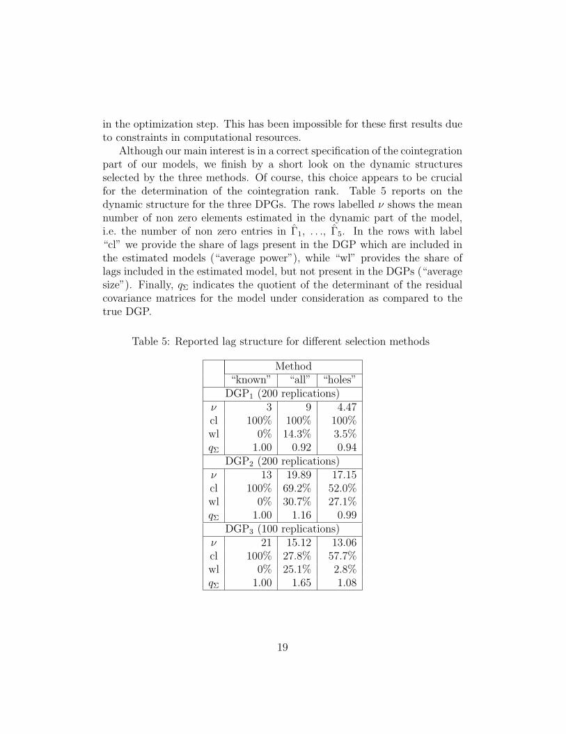
Although our main interest is in a correct specification of the cointegrationpart of our models, we finish by a short look on the dynamic structuresselected by the three methods. Of course, this choice appears to be crucialfor the determination of the cointegration rank. Table 5 reports on thedynamic structure for the three DPGs. The rows labelled ν shows the meannumber of non zero elements estimated in the dynamic part of the model,i.e. the number of non zero entries in Γ1, . . ., Γ5. In the rows with label“cl” we provide the share of lags present in the DGP which are included inthe estimated models (“average power”), while “wl” provides the share oflags included in the estimated model, but not present in the DGPs (“averagesize”). Finally, qΣ indicates the quotient of the determinant of the residualcovariance matrices for the model under consideration as compared to thetrue DGP.

Table 5: Reported lag structure for different selection methods

Method“known” “all” “holes”

DGP1 (200 replications)ν 3 9 4.47cl 100% 100% 100%wl 0% 14.3% 3.5%qΣ 1.00 0.92 0.94

DGP2 (200 replications)ν 13 19.89 17.15cl 100% 69.2% 52.0%wl 0% 30.7% 27.1%qΣ 1.00 1.16 0.99

DGP3 (100 replications)ν 21 15.12 13.06cl 100% 27.8% 57.7%wl 0% 25.1% 2.8%qΣ 1.00 1.65 1.08

19

For a simple dynamic structure like DGP1, the optimization method ap-pears to work extremely well by finding the relevant lags (on the diagonalof Γ1) for all replications and including only a small number of additionallags. The standard method has to include all nine first order lags in orderto capture the relevant lags. Consequently, the share of non relevant lagsincreases as the mean number of lags included (ν = 9). Only for this rathersimple DGP, qΣ indicates a slight tendency of overfitting for the “take all up”approach and – to a smaller extent - for the “holes” method. For the otherDGPs no overfitting is indicated by this measure, but the “holes” approachresults in better fitting models with a determinant of the residual covariancematrix close to that of the true DGP. For DGP2, the share of relevant lagsidentified by the optimization heuristic is smaller than for the “all” heuristic,which is surprising at first sight given the larger search space. This result de-serves further attention. Nevertheless, it is remarkable that the optimizationheuristic seems to identify those lags allowing for a correct estimation of thecointegration rank more often than the “all” heuristic (see Table 4). Finally,for DGP3, the optimization heuristic is much more successful in selecting therelevant lags and avoiding to include non relevant ones. Nevertheless, thisadvantage in the modelling of the dynamic part does not show up in a dra-matic improvement in selecting the right cointegration rank. Again our firstresults support earlier findings that the performance of model selection pro-cedures in the context of cointegration depends heavily on the specific DGP.In particular, as Gredenhoff and Karlsson (1999, p. 184) we might concludethat “choosing the lag–length in VAR–models is not an easy task”. Conse-quently, more research is needed to identify the features of DGPs affectingthe performance of different model selection methods.

5 Conclusion

In this paper, we discuss the model selection issue in the context of non–stationary VAR–models with stationary cointegration relationships. Ourreading of the literature suggests that the modelling of the dynamic partof these VEC–models is crucial for a correct rank identification. We comparedifferent methods for model selection in a MC simulation including methodsbased on information criteria and a two–step procedure employing Johansen’stesting strategy. Furthermore, we introduce a discrete optimization heuris-tic allowing for the selection of lag structures out of a much larger search

20

space than the usual “take all up to the k–th lag” approach. Again, a MCsimulation is used to assess the relative performance of this algorithm.

Our findings support the view that the results of methods aiming at iden-tifying the cointegration rank of a VECM depend heavily on the modelling ofthe dynamic structure. In contrast to earlier studies and in accordance withmore recent findings, already a very small set of DGPs indicates that thiseffect might differ markedly for different DGPs. In particular, the practicalguideline rather to include too many lags is not supported for all DGPs byour findings. However, we find that the optimization heuristic approach incombination with a modified BIC performs relatively well as compared tothe “take all up to the k–th lag” approach.

Given the small set of DGPs considered in this paper and the restriction toa single model selection procedure in the optimization context points directlytowards future research. First, we have to apply our method to a much largerset of different DGPs in order to find out how robust our results are and whichfactors might be responsible for differences in the (relative) performance.Second, we want to include other procedures in our approach, in particularthe modified PIC suggested by Chao and Phillips (1999) and Johansen’sprocedure. Finally, we have to improve the performance of the estimationstep in the optimization heuristic in order to allow for a larger number ofiterations for a given problem in order to have more reliable results from theoptimization method.

Despite our limited and preliminary results the tentative conclusion seemsadmitted that employing a more refined method for identifying the dynamicstructure of a VECM might improve the performance in terms of rank orderidentification.

References

Ahking, F. W. (2002). Model mis–specification and Johansen’s co–integrationanalysis: An application to the US money demand. Journal of Macroe-conomics 24, 51–66.

Ahn, S. K. and G. C. Reinsel (1990). Estimation for partially nonstationarymultivariate autoregressive models. Journal of the American StatisticalAssociation 85(411), 813–823.

21

Bahmani-Oskooee, M. and T. J. Brooks (2003). A new criteria for selectingthe optimum lags in Johansen’s cointegration technique. Applied Eco-nomics 35, 875–880.

Bewley, R. and M. Yang (1998). On the size and power of system tests forcointegration. The Review of Economics and Statistics 80(4), 675–679.

Bruggemann, R., H.-M. Krolzig and H. Lutkepohl (2003). Comparison ofmodel reduction methods for VAR processes. Technical Report 2003–W13. Economics Group, Nuffield College. University of Oxford.

Campos, J., D. F. Hendry and H.-M. Krolzig (2003). Consistent model se-lection by an automatic gets approach. Oxford Bulletin of Economics &Statistics 65(s1), 803–820.

Chao, J. C. and P. C. B. Phillips (1999). Model selection in partially non-stationary vector autoregressive processes with reduced rank structure.Journal of Econometrics 91, 227–271.

Cheung, Y.-.W and K. S. Lai (1993). Finite–sample sizes of Johansen’s like-lihood ratio test for cointegration. Oxford Bulletin of Economics andStatistics 55, 313–328.

Fogel, D. (2001). Evolutionary Computation: Toward a New Philosophy ofMachine Intelligence. 2nd ed.. IEEE Press. New York, NY.

Gatu, Cristian and Erricos J. Kontoghiorghes (2003). Parallel algorithms forcomputing all possible subset regression models using the QR decom-position. Parallel Computing p. forthcoming.

Gonzalo, J. and J.-Y. Pitarakis (1999). Lag length estimation in large dimen-sional systems. Journal of Time Series Analysis 23(4), 401–423.

Gredenhoff, M. and S. Karlsson (1999). Lag–length selection in VAR–modelsusing equal and unequal lag–length procedures. Computational Statistics14, 171–187.

Hendry, D. F. and H.-M. Krolzig (2001). Automatic Econometric Model Se-lection. Timberlake Consultants Press. London.

22

Hendry, D. F. and H.-M. Krolzig (2003). Automatic model selection: A newinstrument for social science. Technical report. Economics Department.Oxford University.

Ho, M. S. and B. E. Sørensen (1996). Finding cointegration rank in highdimesional systems using the Johansen test: An illustration using databased Monte Carlo simulations. The Review of Economics and Statistics78(4), 726–732.

Jacobson, T. (1995). On the determination of lag order in vector autoregres-sions of cointegrated systems. Computational Statistics 10(2), 177–192.

Johansen, S. (1988). Statistical analysis of cointegration vectors. Journal ofEconomic Dynamics and Control 12, 231–254.

Johansen, S. (1991). Estimation and hypothesis testing of cointegra-tion vectors in gaussian vector autoregressive models. Econometrica59(6), 1551–1580.

Johansen, S. (1992). Determination of cointegration rank in the presence ofa linear trend. Oxford Bulletin of Economics and Statistics 54(3), 383–397.

Johansen, S. (1995). Likelihood-Based Inference in Cointegrated Vector Au-toregressive Models. Oxford University Press. Oxford.

Johansen, S. (2002). A small sample correction for the test of cointegra-tion rank in the vector autoregressive model. Econometrica 70(5), 1929–1961.

Krolzig, H.-M. and D. F. Hendry (2001). Computer automation of general–to–specific model selection procedures. Journal of Economic Dynamics& Control 25, 831–866.

Lutkepohl, H. (1993). Introduction to Multiple Time Series Analysis. 2 ed..Springer. Berlin.

Maringer, Dietmar and Peter Winker (2003). Portfolio optimization underdifferent risk constraints with memetic algorithms. Technical Report2003–005E. Staatswissenschaftliche Fakultat. Universitat Erfurt.

23

Moscato, P. (1999). Memetic algorithms: A short introduction. In: New Ideasin Optimization (M. Doriga D. Corne and F. Glover, Eds.). pp. 219–234.MacGraw-Hill. London.

Omtzigt, Pieter (2002). Automatic identification and restriction of the coin-tegration space. Technical Report 2002/25. Faculty of Economics. Uni-versity of Insubria, Varese.

Potscher, B. M. (1991). Effects of model selection on inference. EconometricTheory 7, 7–67.

Winker, Peter (1995). Identification of multivariate AR–models by thresholdaccepting. Computational Statistics and Data Analysis 20(9), 295–307.

Winker, Peter (2000). Optimized multivariate lag structure selection. Com-putational Economics 16, 87–103.

Winker, Peter (2001). Optimization Heuristics in Econometrics: Applicationsof Threshold Accepting. Wiley. Chichester.

24