Optimal hedging with the vector autoregressive model

Lukasz T. Gatarek12 & Søren Johansen3

9 Feb 2014

Abstract

We derive the optimal hedging ratios for a portfolio of assets driven by a Coin-tegrated Vector Autoregressive model with general cointegration rank. Our hedge isoptimal in the sense of minimum variance portfolio.

We consider a model that allows for the hedges to be cointegrated with the hedgedasset and among themselves. We find that the minimum variance hedge for assetsdriven by the CVAR, depends strongly on the portfolio holding period. The hedgeis defined as a function of correlation and cointegration parameters. For short hold-ing periods the correlation impact is predominant. For long horizons, the hedge ratioshould overweight the cointegration parameters rather then short-run correlation in-formation. In the infinite horizon, the hedge ratios shall be equal to the cointegratingvector. The hedge ratios for any intermediate portfolio holding period should be basedon the weighted average of correlation and cointegration parameters.

The results are general and can be applied for any portfolio of assets that can bemodeled by the CVAR of any rank and order.

Keywords: hedging, cointegration, minimum variance portfolio

JEL Classification: C22, C58, G11

1The first author is grateful to National Science Center Poland for funding with grant Preludium No.2013/09/N/HS4/03751. The second author is grateful to CREATES - Center for Research in EconometricAnalysis of Time Series (DNRF78), funded by the Danish National Research Foundation.

2Econometric Institute and Tinbergen Institute, Erasmus University Rotterdam, P.O. Box 1738, NL-3000DR Rotterdam, The Netherlands. E-mail: gatarek@tlen.pl

3Department of Economics, University of Copenhagen and CREATES, Department of Economics andBusiness, Aarhus University, DK-8000 Aarhus C. E-mail: soren.johansen@econ.ku.dk.

1

Introduction

The idea of minimum variance portfolio dates back to [Markowitz, 1952]. It is defined as aportfolio of individually risky assets that, when taken together, result in the lowest possiblerisk level for the rate of expected return. Such a portfolio hedges each investment with anoffsetting investment; the individual investor’s choice on how much to offset investments de-pends on the level of risk and expected return he/she is willing to accept. The investments ina minimum variance portfolio are individually riskier than the portfolio as a whole. The nameof the term comes from how it is mathematically expressed in Markowitz Portfolio Theory,in which volatility is used as a replacement for risk, and in which less variation in volatilitycorrelates to less risk in an investment. Since the seminal paper of [Markowitz, 1952], thenotion of minimum variance portfolio and minimum variance hedging has been explored andextended heavily in both financial and econometric literature, see [Grinold and Kahn, 1999].However, the common denominator of those methods remain the same. They either aim atminimizing volatility of a portfolio itself or volatility of some function of a portfolio. Thisfunction often represents the evolution of the portfolio over time. This is also the purposeof the hedging problem we define.

In general, the hedging methods can be divided in two classes: static and dynamicmethods. The static hedging techniques assume that the hedged portfolio is selected giveninformation available in period t, and remains unchanged during the entire holding periodt, . . . , t + h. On the contrary, the dynamic hedging methods allow for rebalancing of theportfolio during the holding period.

Our method is static. We find the optimal hedging ratios for a portfolio of assets drivenby a Cointegrated Vector Autoregressive model (CVAR). We start with a simple process,which relates the hedged asset to hedges via cointegration relation. The hedges are exogenousand are modeled via random walks. In a general specification of the model, the hedges canalso be related to the hedged asset via cointegration relation.

The general results that we find, define the optimal hedging ratios as a function ofcorrelation and cointegration parameters in the model. We find that a minimum varianceportfolio held for one period should be based on the hedge ratios driven only by correlation.In the infinite horizon, the hedge ratios will be equal to a cointegrating vector. The hedgeratios for any intermediate portfolio holding period should be based on the weighted averageof the correlation and cointegration parameters. Our result are general and can be appliedto a CVAR model of any rank and order.

1 Exogenous case

1.1 Univariate hedge

Regression estimation of a cointegration relation Single regression equation estima-tion of cointegration relation has been a topic of research for more than two decades. Thereare many methods of correcting the finite-sample biases in static regressions. [Phillips, 1988]and [Phillips, 1990] have argued that the performance of estimators of cointegrating vectorsbased on individual regressions is adversely affected by the existence of first-order biases.These biases have no effect on the consistency of the estimators, but result in the asymptoticdistributions having non-zero means.

Such biases might play an important role in finite samples. Let us consider a simple

2

bivariate cointegration model with an endogenous variable y1t cointegrated with a weaklyexogenous variable y2t

y1t = βy2t + u1t

y2t = y2,t−1 + u2t

(1.1)

where where ut are independent identically distributed (i.i.d.) N(0, Φ) random errors withmean zero and variance Φ, where

Φ =

(φ11 φ12

φ21 φ22

).

When disturbances uit, i = 1, 2 are autocorrelated or intercorrelated, a static regression ofy1t on y2t provides an estimate which can be biased in fairly large samples. This is due todisregarding any information about the process generating y2t. Under i.i.d. Gaussian er-rors, the parameters of the process can be estimated via the full-system maximum likelihoodestimation of cointegrated system, or by maximum likelihood of the regression model withparameters (β, Φ). This amounts to a single-equation regression of y1t corrected for y2t−1 andy2t. This method is referred to as a single-equation dynamic regression. The long-run esti-mates obtained from the properly specified dynamic equation are equivalent, asymptotically,to the full system estimates.

For the system in (1.1), the definition of dynamic regression is simple. In what follows wesummarize this procedure. First we substitute in (1.1) using the second equation to obtain

y1t = βy2,t−1 + βu2t + u1t = βy2,t−1 + v1t,

where v1t = βu2t + u1t, and we define βCorr = φ−122 ξ21 = (φ21 + βφ22)φ

−122 . For v2t = u2t we

then have vt i.i.d. N(0, Ξ) where

Ξ =

(ξ11 ξ12

ξ12 ξ22

)=

(φ11 + β2φ22 + 2βφ12 φ12 + βφ22

φ21 + βφ22 φ22

).

From the multivariate Normal theory, the following relation holds

E(v1t|u2t) =Cov(v1t, u2t)

V ar(u2t)u2t = ξ21φ

−122 u2t = βCorru2t,

such that

E(y1t|y2t, y2,t−1) = E(βy2t + v1t|u2t) = βy2t + βCorru2t = βy2t + βCorrΔy2t

results in a regression form of the cointegration model

y1t = βy2,t−1 + βCorrΔy2t + η1t. (1.2)

Here βCorr = φ−122 ξ21 collects the information with respect to the correlation between v1t

and u2t and corrects the estimate from a single equation by information about the correla-tion structure among random errors. We will refer to it as a β-correction parameter. Byconstruction ηt = y1t−E(y1t|y2t, y2,t−1) is an i.i.d. sequence independent of the sequence u2t.

3

The single equation in (1.2) represents unbiased estimation of the cointegration parameterβ. We can prove that the correction works by analyzing covariance of ηt and u2t. Byconstruction of ηt

ηt = u1t − φ21φ−122 u2t,

we find no covariance between ηt and u2t

Cov(ηt, u2t) = E((u1t − φ12φ−122 u2t), u2t) = φ12 − φ12φ

−122 φ22 = 0,

what implies that running dynamic regression (with y2t and y2,t−1) leads to no loss of infor-mation from φ12. The variance of ηt is given by

V ar(ηt) = E(u1t − φ12φ−122 u2t)

2 = φ11 − φ12φ−122 φ21.

Several features are now evident. By construction ηt is uncorrelated with u2t. The processu2t is serially uncorrelated with past u2t and with past u1t. It follows that ηt and u2t areuncorrelated at all lags. The covariance matrix of (v1t, u2t)

′ is diagonal, and the estimation ofa single dynamic equation provides a fully efficient and unbiased estimate of the cointegrationparameter β. Traditionally βCorr is disregarded after running the regression in (1.2). Its mainand only role is to provide an unbiased estimator of β. The information that is conveyedby this parameter, however, might be useful on its own. In what follows we will presentan example of how it can be used in construction of hedged portfolios for assets modeledaccording to the specification in (1.1).

Hedging under full mean reversion Model (1.1) can be interpreted as a realistic rep-resentation of the data generating process for prices of pairs of assets in many financialmarkets. In that case the process y1t is endogenous and its realization cointegrates withthe path of y2t with cointegrating parameter β. The process y2t is defined as an exogenousrandom walk. Apart from cointegration between y1t and y2t, the process is also characterizedby intercorrelation in the disturbances. Despite widely used volatility models in financialeconometric theory, cointegrated systems with independent and identically distributed errorsremain a valid representation of various relations in financial market, such as daily measure-ment of financial instruments with limited liquidity. An illiquid asset can be defined as anasset which cannot readily be sold at its face value, see [Vayanos, 2004]. The price formationprocess in such markets underlie different principles than the highly volatile intra-day, highfrequency trading environments. For illiquid markets, the volatility clustering patterns etc.,are not reflected in the price quotations. That concerns to an even higher extent quotedfinancial contracts, whose maturity is distant in the future, for instance in 2 or 3 years. Suchfamilies of future contracts, each with different maturity, but referring to the same under-lying asset, can be modeled by common stochastic trends. Apart from that, the amountof correlation among such assets is naturally very high. This is related to the sparsity ofobservations (due to illiquidity), what implies a small amount of noise at the level of dailymeasurements. In such systems, hedging of a particular maturity with closer or further ma-turities, has remained a financial industry standard for decades. The informational content,filtered by price quotations for different maturities, remains unchanged across maturity, onlythe amount and speed of adjustment of distinct maturities to the common market trend isdifferent. Due to limited volatility in such markets, such systems can be well representedby the specification in (1.1), with reservation, however, that the strong assumption about

4

the full reversion in this model should be relaxed. The simplistic specification in model(1.1) implies full mean reversion from period to period. This follows from an alternativerepresentation of the model in (1.1) given by

Δy1t = αy1,t−1 + βy2t + u1t

Δy2t = u2t,(1.3)

where α = −1 and Δy1t = y1t − y1,t−1. This representation of the system in (1.1) is referredto as an error correction form, where α can be interpreted as mean reversion or speed ofadjustment. Estimation of the parameter α constitutes an important part of econometricmodeling in cointegrated systems. For expository reasons we start with the rather restrictivespecification of full reversion, α = −1, which will be replaced by a more general model below.We derive first an optimal hedge for a model with full mean reversion.

As shown above, the regression estimation of model (1.1) requires a correlation correctionrepresented by the parameter βCorr. The information contained in this parameter can beinformative for a hedging procedure based on this process. Our goal consists of finding aminimum variance portfolio. In what follows, we define this hedge in detail given the datagenerating process for assets specified by the equations (1.1).

We define the hedging parameter βh as the amount invested in the hedge y2t in order tohedge asset y1t and thus we define the portfolio in time period t

st = y1t − βhy2t (1.4)

which consists of assets y1t and y2t weighted with (1,−βh)′. The subscript h indicates that

the main determinant of the hedge we define is the portfolio holding period denoted by h.In financial market one can consider a long and a short position in a given security. The

long position means the holder of the position owns the security and will profit if the price ofthe security goes up. The short position is defined as the sale of a borrowed security, with theexpectation that the asset will fall in value. Then, the investor must eventually return theborrowed security by buying it back from the market. Because it can be purchased cheaperthen at the time of borrowing, the difference in price results in profit for the investor.

In portfolio hedging, traditionally a long position in asset y1t is hedged with short aposition in another asset y2t and vice versa. Thus the sign in front of the weight βh symbolizesthe market convention regarding hedging practice.

Over time the portfolio value can change. Let st+h − st denote the change in portfoliomarket value, induced by the risk drivers we wish to hedge against. Provided a hedge y2t isavailable, the hedging problem involves computing the vector of portfolio weights (1,−βh)

′

that is optimal according to a particular method. The choice of method depends on theobjective of the portfolio manager. Although those objectives can be various, in most casesthey aim at keeping the risk caused by the unhedged part of y1t minimal over time. Themarket value of the portfolio defines the exposure of the portfolio, which can be interpretedas an unhedged part of y1t in period t. This invokes an alternative interpretation of theportfolio value as a spread

st = y1t − βhy2t. (1.5)

Further we define a hedging error after h observations as

et(h) = st+h − st = y1,t+h − y1t − βh(y2,t+h − y2t). (1.6)

5

The hedging problem we consider aims at minimizing the conditional variance of thehedging error for a holding period h given the past information It = σ(ys, s ≤ t}.

The optimization problem is defined as

minβh

V ar(et(h)|It) = minβh

V ar(st+h|It). (1.7)

The optimal portfolio is selected in period t and it is held up to period t + h. It is a statichedge, as the portfolio is not rebalanced during periods t, . . . , t + h.

We present an optimal hedge which explores both the long term cointegration parameterβ, but also the correlation between the random errors in y1t and y2t.

Theorem 1.1 Let yt, t = 1, . . . , T, be bivariate and given by

y1t = βy2t + u1t,

y2t = y2,t−1 + u2t,

where ui are i.i.d. (0, Φ). Then the optimal hedge coefficient for the portfolio st = y1t −βhy2t

at time horizon h is given by

β∗h = β + h−1φ−1

22 φ21 = h−1(β(h − 1) + βCorr), (1.8)

and the minimal variance is

V ar(y1,t+h − β∗hy2,t+h|It) = φ11 − h−1φ12φ

−122 φ21.

Proof: See Appendix.The hedge defined in (1.8) is a weighted average of the correlation correction, βCorr, and

the cointegration parameter with weights: 1/h and (h−1)/h. The resulting formula complieswith the stylized facts about the short- and long-term hedging in the sense that for a shortperiod, h = 1, we hedge fully based on the correlation

β⋆h = βCorr,

whereas for a long period, when h → ∞, we hedge fully based on cointegration

β⋆h = β.

1.2 Multivariate Specification

Regression estimation of cointegration relation We define the model with n assets,from which n − 1 are hedges. Let yt = (y1t, y

′2t)

′ ∈ R1+(n−1), t = 1, . . . , T be given by

y1t = β′y2t + u1t

y2t = y2t−1 + u2t,(1.9)

where ui are i.i.d. (0, Φ). The main difference between the univariate case (with one hedgemodeled as a random walk y2t) and the multivariate case, is the possibility of correlationbetween the innovations of the random walks y2t, y3t, . . . , ynt. Two hedges modeled by cor-related random walks are substitutes. In the extreme scenario, if two potential hedges are

6

fully correlated, then having one of them to hedge y1t is enough for a portfolio. The optimalhedges that we derive for the portfolio based on assets modeled according to (1.9) takesinto account not only the ratio between the cointegration and correlation parameters butalso deeply explores the correlation in order to account for optimal amount of hedges in aportfolio. By comparing the variance of the optimal portfolio we can see what we gain byincluding more hedges.

To derive the composition of the hedging portfolio, we first need to derive the β-correctionparameters, representing the presence of correlation in the errors in the multivariate spec-ification. As we allow for n − 1 cointegrating parameters βi, i ∈ 2, . . . , n, we need n − 1correction parameters. To derive them we follow the same procedure as in the single hedgescenario. We insert the random walks in y2 into first equation in (1.9). The resulting equationfor y1t can be specified as

y1t = β′y2t + β′u2t + u1t,

= β′y2t + v1t

where v1t = β′u2t + u1t. Similarly to the univariate case, in order to define the correctionparameters, we explore the covariance between v1t and u2t. We obtain

V ar

(v1t

u2t

)=

(β′Φ22β + β′Φ21 + Φ12β Φ12 + β′Φ22

Φ21 + Φ22β Φ22

)Based on properties of the multivariate Normal distribution we obtain

E(v1t|u2t) = (β + Φ−122 Φ21)u2t

soy1t = β′y2t + βCorr′Δy2t + ηt,

whereβCorr = β + Φ−1

22 Φ21,

and {ηt} is i.i.d. and uncorrelated with {u2t}.Hedging with correlated assets The vector containing the n − 1 individual hedges isdefined as

βh = (βh,2, . . . , βh,n)′.

Then the portfolio is defined asst = y1t − β′

hy2t. (1.10)

We interpret βh,i, i ∈ 2, . . . , n as the amount of asset yit, necessary to hedge y1t in theportfolio st. Further, the unhedged part of y1t is again equal to the value (exposure) of theportfolio

st = y1t − β′hy2t,

and the hedging error over h periods is defined as in (1.6). The optimal hedge that minimizesthe variance of the hedging error over h periods follow.

7

Theorem 1.2 Let yt = (y1t, y′2t)

′ ∈ R1+(n−1), t = 1, . . . , T be given by

y1t = β′y2t + u1t,

y2t = y2t−1 + u2t,

where ui are i.i.d. (0, Φ). Then the optimal hedge coefficient for the portfolio st = y1t −β′hy2t

at time horizon h is given by

β∗h = β + h−1Φ−1

22 Φ21 = h−1(β(h − 1) + βCorr),

and the minimal variance is

V ar(y1,t+h − β∗hy2,t+h|It) = Φ11 − h−1Φ12Φ

−122 Φ21.

Proof: See Appendix.It is seen that the variance of the optimal portfolio increases with the horizon h, from

the conditional variance of u1t given u2t, Φ11 − Φ12Φ−122 Φ21 for h = 1, to the variance of the

cointegrating relation Φ11 for h → ∞. It is also seen that including more correlated hedges,the varian of u1t given u2t will decrease, but the limit remains the same.

2 Full cointegration model

The analysis under exogenous hedges is now generalized to the full cointegration model, see[Johansen 1996]. Thus we consider a model that allows the hedges to be cointegrated withy1t and among themselves such that the number of cointegrating relations could be morethan one. The assumption of full reversion is dropped and general adjustment coefficientsare allowed.

Theorem 2.1 Let (y1t, y′2t)

′ ∈ R1+(n−1), t = 1, . . . , T be given by

Δyt = αγ′yt−1 + ut,

where ut are i.i.d.(0, Ξ) and α and γ are r×n matrices, and the eigenvalues of ρ = Ir+γ′α areinside the unit circle. Then the optimal hedge for the portfolio st = y1t−β′

hy2t = (1,−β′h)

′yt+h

at time horizon h is given byβ∗

h = Σ−1h22Σh21,

where

Σh = V ar(yt+h|It) =

(Σh11 Σh12

Σh21 Σh22

)is given by

Σh = hCΞC ′ − α(γ′α)−2(Ir − ρh)γ′ΞC ′ − CΞγ(Ir − ρ′h)(α′γ)−2α′ (2.1)

+ α(γ′α)−1[h−1∑i=0

ρiγ′Ξγρ′i](α′γ)−1α′,

and C = γ⊥(α′⊥γ⊥)−1α′

⊥. The minimal variance is

V ar(y1,t+h − β∗hy2,t+h|It) = Σh11 − Σh12Σ

−1h22Σh21.

8

Proof: See Appendix.Note that for h = 1, we get Ir − ρ = −γ′α and C + α(γ′α)−1γ′ = In and therefore

Σ1 = CΞC ′ + α(γ′α)−1γ′ΞC ′ + CΞγ(α′γ)−1α′ + α(γ′α)−1γ′Ξγ(α′γ)−1α′ = Ξ,

and for h → ∞ we find h−1Σh = CΞC ′, the long run-variance of the process yt.In the following we assume that there is a cointegrating relation of the form y1t + β′

1y2t,and that the cointegrating vectors have been written as

γ = (γ1, γ2) =

(1 0β1 β2

)(2.2)

for γ1 ∈ Rn and γ2 ∈ Rn×(r−1), and we define

Γ = V ar(γ′yt) = V ar

(y1t + β′

1y2t

β′2y2t

)=

(Γ11 Γ12

Γ21 Γ22

). (2.3)

Theorem 2.2 If the cointegrating relations are given by (2.2) then the variance of the sta-tionary relation y1t − β′y2t is minimized for

β∗coint = −β1 + β2Γ

−122 Γ21. (2.4)

Proof: See Appendix.We finally show that the optimizing portfolio β∗

h = Σ−1h22Σh21, see (2.1), converges to β∗

coint

for h → ∞.

Theorem 2.3 The optimizing portfolio approaches the cointegration portfolio

β∗h → β∗

coint for h → ∞. (2.5)

Proof: See Appendix.

2.1 Some special cases

The results in Theorem 2.1 cover the cases considered so far, in particular we focus on amodel with one cointegrating relation and n − 1 exogenous hedges.

We consider the model (1.3) written in error correction form

Δy1t = α1(y1,t−1 + α−11 β′y2t−1) + β′u2t + u1t

Δy2t = u2t

where ut are i.i.d.(0, Φ). We find the covariance matrix

Ξ = V ar

(β′u2t + u1t

u2t

)=

(Φ11 + β′Φ21 + Φ12β + β′Φ22β β′Φ22 + Φ12

Φ21 + Φ22β Φ22

),

and the parameters α = (α1, 0, . . . , 0)′, γ = (1, α−11 β′)′, γ′

⊥ = (−α−11 β, In−1) and α′

⊥ =(0, In−1), but also

C = In − α(γ′α)−1γ′ =

(0 −α−1

1 β′

0 In−1

).

9

Inserting into the general expression (2.1) we first find that because α′⊥ = (0, In−1) we

getΣh22 = hα′

⊥Ξα⊥ = hΦ22.

Next we see that α′⊥C = α′

⊥ = (0, In−1), 1 + ρ = 1 + γ′α = 1 + α1, C ′e1 = (0,−α−11 β′) and

we find

Σh21 = α′⊥Σhei = hα′

⊥Ξ(0,−α−11 β′) − α′

⊥Ξγ(1 − (1 + α1)h)α−1

1

= −hΦ22βα−11 − (Φ21 + Φ22β + α−1

1 Φ22β)(Ir − (1 + α1)h)α−1

1

and therefore

β∗h = −βα−1

1 + h−1(Φ−122 Φ21 + β(1 + α−1

1 ))((1 + α1)h − 1)α−1

1 . (2.6)

In particular we can take α1 = −1, see (1.1), and find the full mean reversion case whichgives

β∗h = β + h−1Φ−1

22 Φ21,

see Theorem 1.2.

3 Numerical illustrations

3.1 Full mean reversion

To present how the developed methodology works in practice, we present the optimal hedgeimplied by the resulting formulas for a selection of model specifications. It is shown how theoptimal hedging formula balances the correlation and cointegration parameters dependingon the protfolio holding period h. As shown in formula (1.8), for infinitely held portfolios, theoptimal hedge is given by the cointegration parameter. This parameter results in a stationaryportfolio st with a constant variance. Any other selection of the hedging parameter leads toa portfolio which is nonstationary in variance. That is also true about the optimal hedgewe derive for any holding horizon h different from h = ∞. Still, we intend to constructthe portfolio according to the optimal ratio β∗

h implied by the formula, because for a givenholding period h, it results in lower variance than the portfolio based on cointegration hedgeand held h time periods. It is crucial for the methodology to know a priori the holdinghorizon for this portfolio.

To start with, we show the role of strength of correlation for the construction of theoptimal hedge. We start with case of no correlation in random errors of process in (1.1) andthen we increase the correlation subsequently

• No covariance of the innovationsWe select the following parameters for model (1.1)

β = 0.4

Φ =

(0.1 00 0.2

).

(3.1)

These parameters imply the following βCorr parameter

βCorr = ξ21φ−122 = (φ21 + βφ22)φ

−122 = β = 0.4, (3.2)

10

which, according to (1.8), defines the optimal hedge ratio for a portfolio st held up toperiod t + 1, that is, for h = 1. In this degenerate case, the optimal hedge for h = 1,i.e. βCorr, is equal to β. As a consequence

β⋆h =

βCorr + β(h − 1)

h= β. (3.3)

To understand why the relation βCorr = β holds under no covariance in innovationswe need to refer to the regression representation of cointegration

y1t = βy2t−1 + βCorrΔy2t + ηt (3.4)

and the definition of process ηt

ηt = u1t − φ21φ−122 u2t|φ21=0 = u1t. (3.5)

After substituting for ηt in (3.4) we obtain

y1t = βy2t−1 + βCorry2t − βCorry2,t−1 + u1t. (3.6)

It follows immediately that only if βCorr = β we obtain the original equation for y1t inmodel (1.1), i.e.

y1t = βy2t + u1t. (3.7)

• Low covariance of the innovationsIn this scenario we keep the cointegration relation at the same level as in the pre-vious example, but we allow for some correlation in the innovations. The followingparameters are selected for model (1.1)

β = 0.4

Φ =

(0.1 0.010.01 0.2

).

(3.8)

These parameters imply the following βCorr

βCorr = ξ21φ−122 = (φ21 + βφ22)φ

−122 = (0.01 + 0.4 × 0.2)0.2−1 = 0.45. (3.9)

Thus the optimal hedge for h = 1 equals to βCorr = 0.45 and then it smoothly dropsto asymptotically reach the level of the cointegration hedge β = 0.4. Any intermedi-ate portfolio holding horizon h requires a weighted average of those two parameters,according to equation (1.8).

• High covariance in the innovationsFinally we consider scenario of high correlation, implied by the covariance of 0.12. Thefollowing parameters are selected for model (1.1)

β = 0.4

Φ =

(0.1 0.120.12 0.2

).

(3.10)

11

In that case an optimal hedge required for h = 1 rises as much as to 1, higher then inthe previous scenario, where βCorr = 0.45. Thus, the higher correlation automaticallytranslates into a higher hedge for the optimal portfolio for h = 1

βCorr = ξ21φ−122 = (φ21 + βφ22)φ

−122 = (0.12 + 0.4 × 0.2)0.2−1 = 1. (3.11)

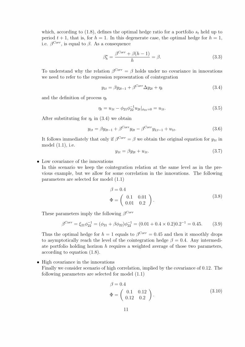
Due to unchanged cointegration parameter, the optimal hedge for an infinitely heldportfolio remains the same, i.e. β = 0.4.

3.2 Limited reversion

• No covariance in the innovationsSimilarly to case of full mean reversion, we start with the scenario of no correlation.We consider the model in (1.3). Mean reversion is set equal to α = −0.2. Cointegrationlevel and covariance matrix are unchanged from the previous example

α = −0.2

β = 0.4

Φ =

(0.1 00 0.2

) (3.12)

which results in the same level of βCorr, as well. The limiting level of the hedge forh → ∞ is immediately found from equation (2.6)

βh(h → ∞) = −β

α= − 0.4

−0.2= 2. (3.13)

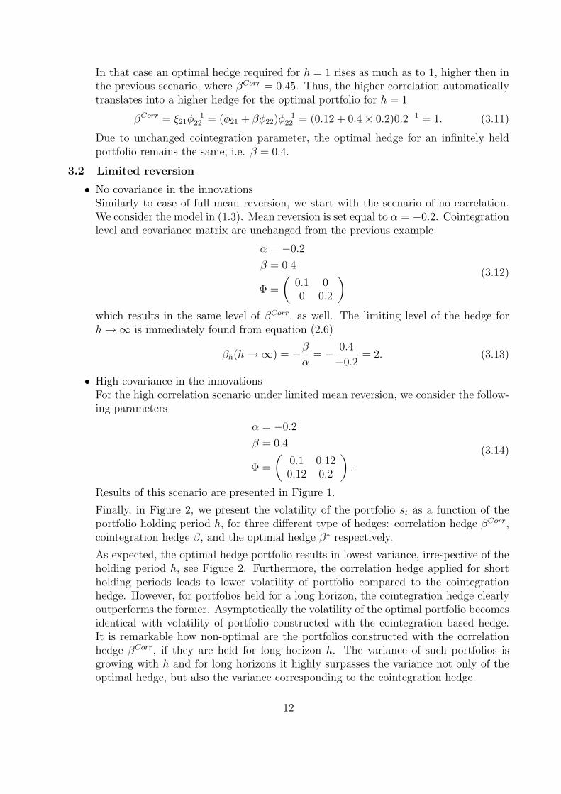
• High covariance in the innovationsFor the high correlation scenario under limited mean reversion, we consider the follow-ing parameters

α = −0.2

β = 0.4

Φ =

(0.1 0.120.12 0.2

).

(3.14)

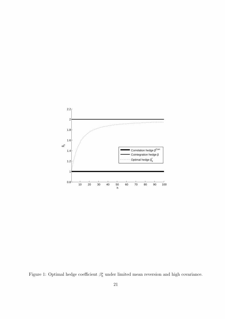
Results of this scenario are presented in Figure 1.

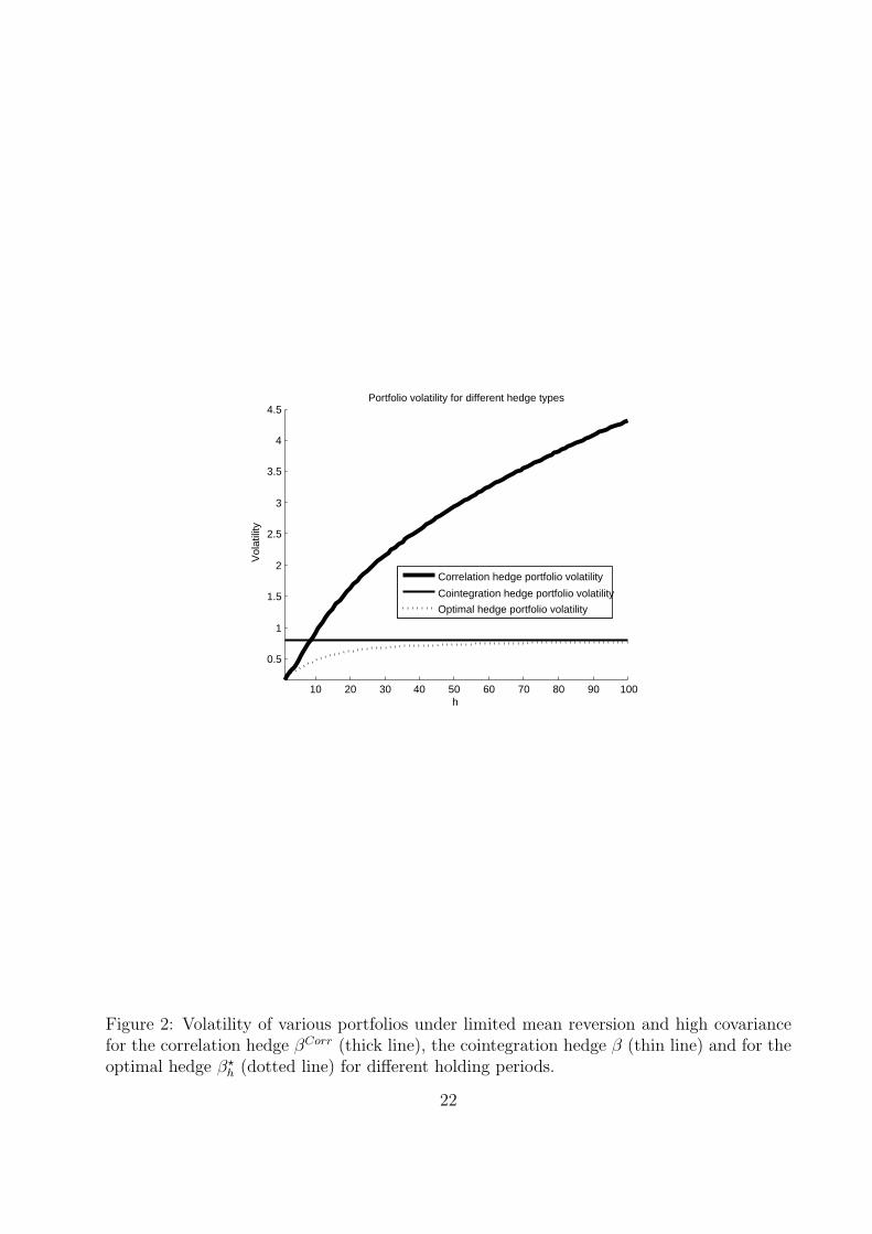
Finally, in Figure 2, we present the volatility of the portfolio st as a function of theportfolio holding period h, for three different type of hedges: correlation hedge βCorr,cointegration hedge β, and the optimal hedge β∗ respectively.

As expected, the optimal hedge portfolio results in lowest variance, irrespective of theholding period h, see Figure 2. Furthermore, the correlation hedge applied for shortholding periods leads to lower volatility of portfolio compared to the cointegrationhedge. However, for portfolios held for a long horizon, the cointegration hedge clearlyoutperforms the former. Asymptotically the volatility of the optimal portfolio becomesidentical with volatility of portfolio constructed with the cointegration based hedge.It is remarkable how non-optimal are the portfolios constructed with the correlationhedge βCorr, if they are held for long horizon h. The variance of such portfolios isgrowing with h and for long horizons it highly surpasses the variance not only of theoptimal hedge, but also the variance corresponding to the cointegration hedge.

12

4 Summary

We derive the optimal hedging ratios for a portfolio of assets driven by a Cointegrated VectorAutoregressive model with general cointegration rank. Our hedge is optimal in the sense ofminimum variance portfolio. We start with the exogenous case, in which the hedged assetdepends on hedges via a cointegration relation, and the hedges are exogenous, modeled byrandom walks. Then we consider a model that allows for the hedges to be cointegratedwith the hedged asset and among themselves. We find that the minimum variance hedge forassets driven by the CVAR, depends strongly on the portfolio holding period. The hedge isdefined as a function of correlation and cointegration parameters. For short holding periodsthe correlation impact is predominant. For long horizons, the hedge ratio should overweightthe cointegration parameters rather then short-run correlation information. In the infinitehorizon, the hedge ratios shall be equal to the cointegrating vector. The hedge ratios for anyintermediate portfolio holding period should be based on the weighted average of correlationand cointegration parameters.

Our results are general and can be applied for any portfolio of assets that can be modeledby the CVAR of any rank and order. The further research aims at a dynamic version of thedeveloped methodology. In that case the static hedge kept for the entire portfolio holdinghorizon shall be replaced by a hedge that is dynamically rebalanced during this period.

13

References

[Grinold and Kahn, 1999] Grinold, R., Kahn, R., (1999), Active Portfolio Management:A Quantitative Approach for Producing Superior Returns andControlling Risk, McGraw-Hill, New York

[Johansen 1996] Likelihood-Based Inference in Cointegrated Vector AutoregressiveModels. Oxford University Press, Oxford (2. ed.)

[Markowitz, 1952] Markowitz, H., (1952), Portfolio selection, Journal of Finance,77-90, 7(1).

[Phillips, 1988] Phillips, P.C.B., (1988), Reflections on econometric methodol-ogy, Economic Record, 64, 344-359.

[Phillips, 1990] Phillips, P.C.B., (1990), Optimal inference in co-integrated sys-tems, Econometrica, 59, 282-306.

[Vayanos, 2004] Vayanos, D., (2004), Flight to Quality, Flight to Liquidity, andthe Pricing of Risk, NBER Working Paper, 10327.

14

Appendix

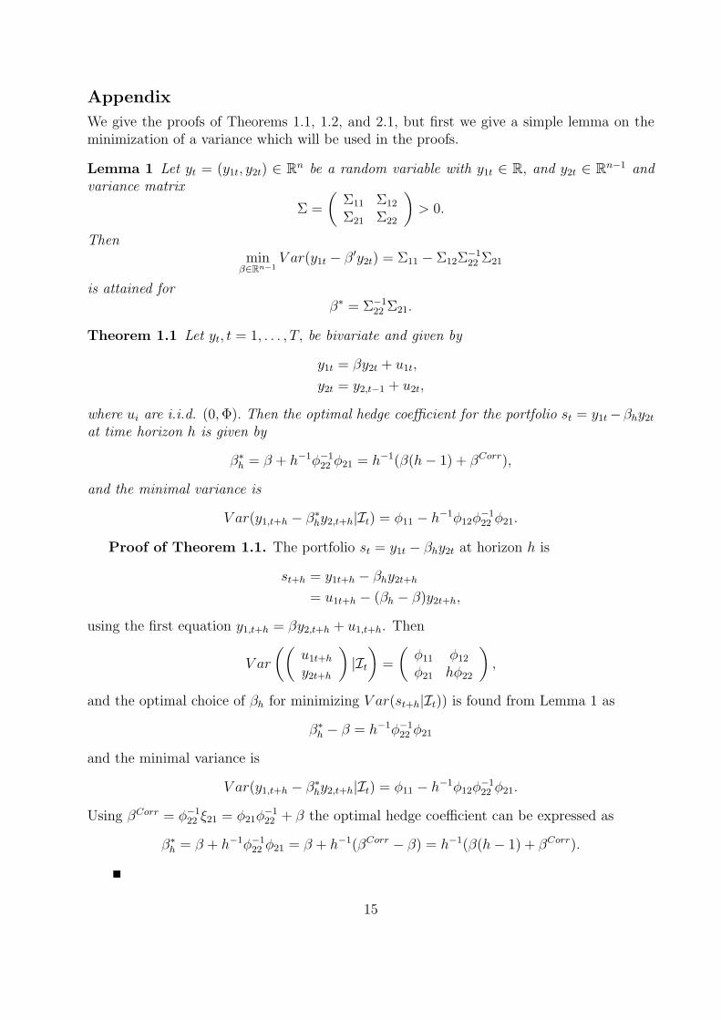
We give the proofs of Theorems 1.1, 1.2, and 2.1, but first we give a simple lemma on theminimization of a variance which will be used in the proofs.

Lemma 1 Let yt = (y1t, y2t) ∈ Rn be a random variable with y1t ∈ R, and y2t ∈ Rn−1 andvariance matrix

Σ =

(Σ11 Σ12

Σ21 Σ22

)> 0.

Thenmin

β∈Rn−1V ar(y1t − β′y2t) = Σ11 − Σ12Σ

−122 Σ21

is attained forβ∗ = Σ−1

22 Σ21.

Theorem 1.1 Let yt, t = 1, . . . , T, be bivariate and given by

y1t = βy2t + u1t,

y2t = y2,t−1 + u2t,

where ui are i.i.d. (0, Φ). Then the optimal hedge coefficient for the portfolio st = y1t −βhy2t

at time horizon h is given by

β∗h = β + h−1φ−1

22 φ21 = h−1(β(h − 1) + βCorr),

and the minimal variance is

V ar(y1,t+h − β∗hy2,t+h|It) = φ11 − h−1φ12φ

−122 φ21.

Proof of Theorem 1.1. The portfolio st = y1t − βhy2t at horizon h is

st+h = y1t+h − βhy2t+h

= u1t+h − (βh − β)y2t+h,

using the first equation y1,t+h = βy2,t+h + u1,t+h. Then

V ar

((u1t+h

y2t+h

)|It

)=

(φ11 φ12

φ21 hφ22

),

and the optimal choice of βh for minimizing V ar(st+h|It)) is found from Lemma 1 as

β∗h − β = h−1φ−1

22 φ21

and the minimal variance is

V ar(y1,t+h − β∗hy2,t+h|It) = φ11 − h−1φ12φ

−122 φ21.

Using βCorr = φ−122 ξ21 = φ21φ

−122 + β the optimal hedge coefficient can be expressed as

β∗h = β + h−1φ−1

22 φ21 = β + h−1(βCorr − β) = h−1(β(h − 1) + βCorr).

15

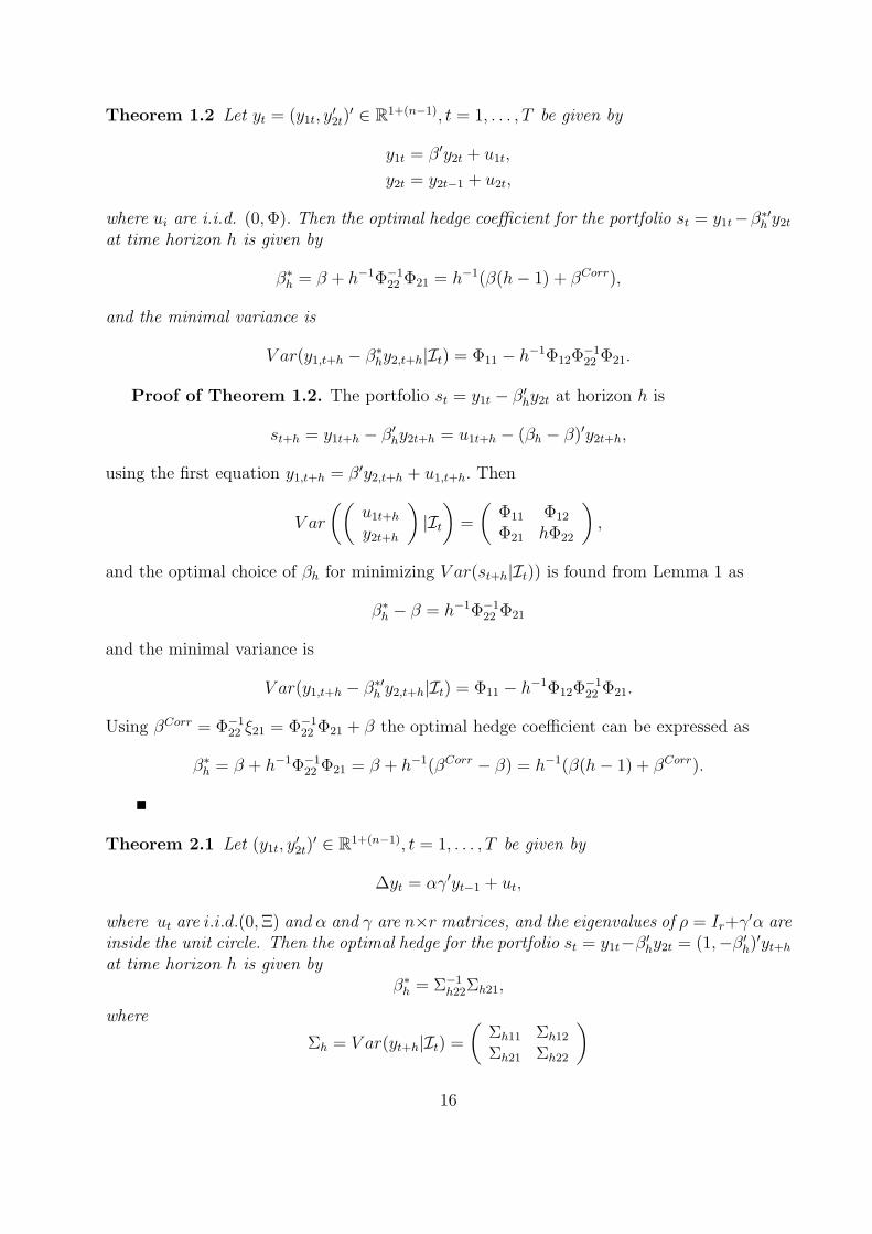
Theorem 1.2 Let yt = (y1t, y′2t)

′ ∈ R1+(n−1), t = 1, . . . , T be given by

y1t = β′y2t + u1t,

y2t = y2t−1 + u2t,

where ui are i.i.d. (0, Φ). Then the optimal hedge coefficient for the portfolio st = y1t−β∗′h y2t

at time horizon h is given by

β∗h = β + h−1Φ−1

22 Φ21 = h−1(β(h − 1) + βCorr),

and the minimal variance is

V ar(y1,t+h − β∗hy2,t+h|It) = Φ11 − h−1Φ12Φ

−122 Φ21.

Proof of Theorem 1.2. The portfolio st = y1t − β′hy2t at horizon h is

st+h = y1t+h − β′hy2t+h = u1t+h − (βh − β)′y2t+h,

using the first equation y1,t+h = β′y2,t+h + u1,t+h. Then

V ar

((u1t+h

y2t+h

)|It

)=

(Φ11 Φ12

Φ21 hΦ22

),

and the optimal choice of βh for minimizing V ar(st+h|It)) is found from Lemma 1 as

β∗h − β = h−1Φ−1

22 Φ21

and the minimal variance is

V ar(y1,t+h − β∗′h y2,t+h|It) = Φ11 − h−1Φ12Φ

−122 Φ21.

Using βCorr = Φ−122 ξ21 = Φ−1

22 Φ21 + β the optimal hedge coefficient can be expressed as

β∗h = β + h−1Φ−1

22 Φ21 = β + h−1(βCorr − β) = h−1(β(h − 1) + βCorr).

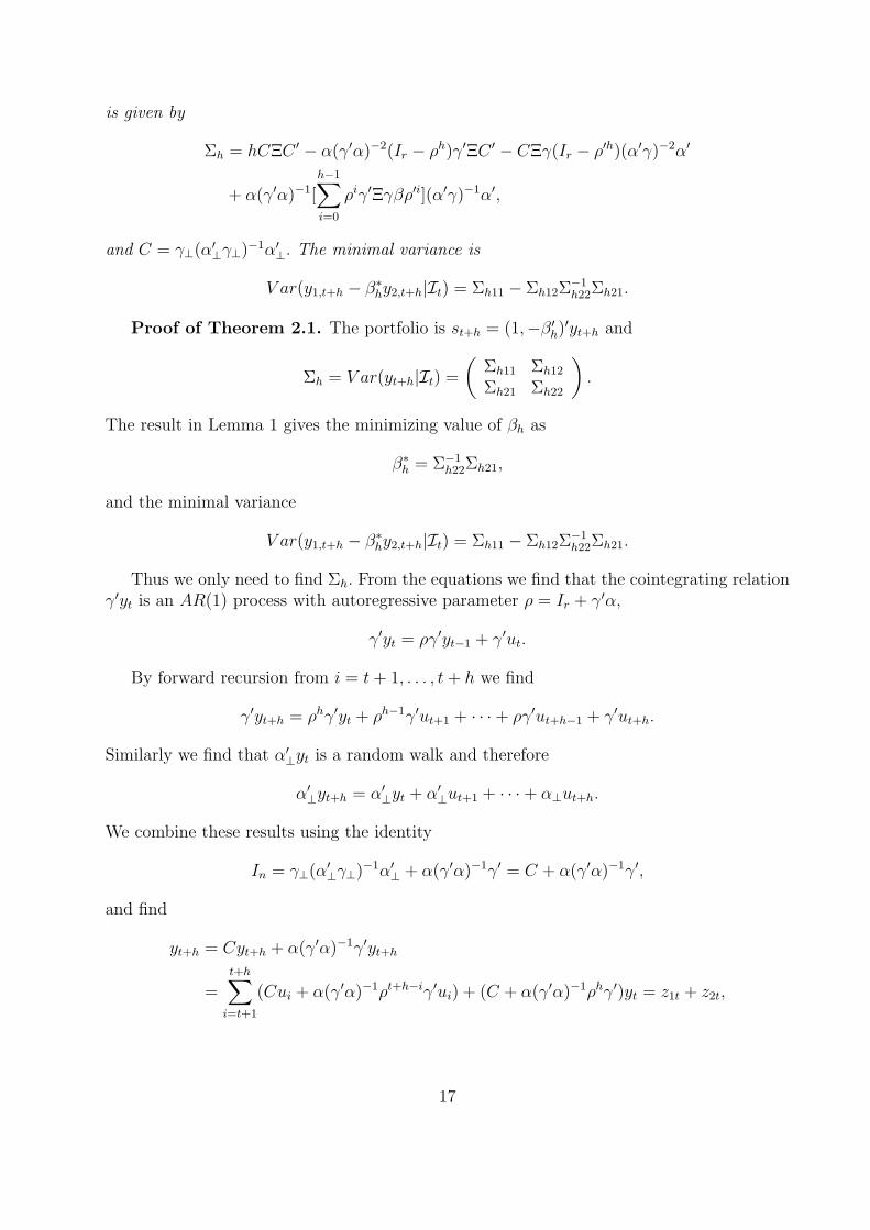
Theorem 2.1 Let (y1t, y′2t)

′ ∈ R1+(n−1), t = 1, . . . , T be given by

Δyt = αγ′yt−1 + ut,

where ut are i.i.d.(0, Ξ) and α and γ are n×r matrices, and the eigenvalues of ρ = Ir+γ′α areinside the unit circle. Then the optimal hedge for the portfolio st = y1t−β′

hy2t = (1,−β′h)

′yt+h

at time horizon h is given byβ∗

h = Σ−1h22Σh21,

where

Σh = V ar(yt+h|It) =

(Σh11 Σh12

Σh21 Σh22

)

16

is given by

Σh = hCΞC ′ − α(γ′α)−2(Ir − ρh)γ′ΞC ′ − CΞγ(Ir − ρ′h)(α′γ)−2α′

+ α(γ′α)−1[h−1∑i=0

ρiγ′Ξγβρ′i](α′γ)−1α′,

and C = γ⊥(α′⊥γ⊥)−1α′

⊥. The minimal variance is

V ar(y1,t+h − β∗hy2,t+h|It) = Σh11 − Σh12Σ

−1h22Σh21.

Proof of Theorem 2.1. The portfolio is st+h = (1,−β′h)

′yt+h and

Σh = V ar(yt+h|It) =

(Σh11 Σh12

Σh21 Σh22

).

The result in Lemma 1 gives the minimizing value of βh as

β∗h = Σ−1

h22Σh21,

and the minimal variance

V ar(y1,t+h − β∗hy2,t+h|It) = Σh11 − Σh12Σ

−1h22Σh21.

Thus we only need to find Σh. From the equations we find that the cointegrating relationγ′yt is an AR(1) process with autoregressive parameter ρ = Ir + γ′α,

γ′yt = ργ′yt−1 + γ′ut.

By forward recursion from i = t + 1, . . . , t + h we find

γ′yt+h = ρhγ′yt + ρh−1γ′ut+1 + · · · + ργ′ut+h−1 + γ′ut+h.

Similarly we find that α′⊥yt is a random walk and therefore

α′⊥yt+h = α′

⊥yt + α′⊥ut+1 + · · · + α⊥ut+h.

We combine these results using the identity

In = γ⊥(α′⊥γ⊥)−1α′

⊥ + α(γ′α)−1γ′ = C + α(γ′α)−1γ′,

and find

yt+h = Cyt+h + α(γ′α)−1γ′yt+h

=t+h∑

i=t+1

(Cui + α(γ′α)−1ρt+h−iγ′ui) + (C + α(γ′α)−1ρhγ′)yt = z1t + z2t,

17

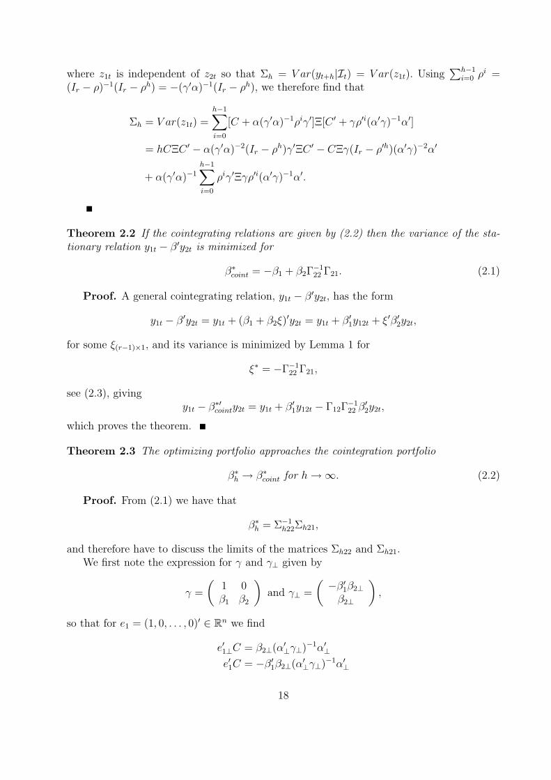
where z1t is independent of z2t so that Σh = V ar(yt+h|It) = V ar(z1t). Using∑h−1

i=0 ρi =(Ir − ρ)−1(Ir − ρh) = −(γ′α)−1(Ir − ρh), we therefore find that

Σh = V ar(z1t) =h−1∑i=0

[C + α(γ′α)−1ρiγ′]Ξ[C ′ + γρ′i(α′γ)−1α′]

= hCΞC ′ − α(γ′α)−2(Ir − ρh)γ′ΞC ′ − CΞγ(Ir − ρ′h)(α′γ)−2α′

+ α(γ′α)−1

h−1∑i=0

ρiγ′Ξγρ′i(α′γ)−1α′.

Theorem 2.2 If the cointegrating relations are given by (2.2) then the variance of the sta-tionary relation y1t − β′y2t is minimized for

β∗coint = −β1 + β2Γ

−122 Γ21. (2.1)

Proof. A general cointegrating relation, y1t − β′y2t, has the form

y1t − β′y2t = y1t + (β1 + β2ξ)′y2t = y1t + β′

1y12t + ξ′β′2y2t,

for some ξ(r−1)×1, and its variance is minimized by Lemma 1 for

ξ∗ = −Γ−122 Γ21,

see (2.3), givingy1t − β∗′

cointy2t = y1t + β′1y12t − Γ12Γ

−122 β′

2y2t,

which proves the theorem.

Theorem 2.3 The optimizing portfolio approaches the cointegration portfolio

β∗h → β∗

coint for h → ∞. (2.2)

Proof. From (2.1) we have that

β∗h = Σ−1

h22Σh21,

and therefore have to discuss the limits of the matrices Σh22 and Σh21.We first note the expression for γ and γ⊥ given by

γ =

(1 0β1 β2

)and γ⊥ =

(−β′

1β2⊥β2⊥

),

so that for e1 = (1, 0, . . . , 0)′ ∈ Rn we find

e′1⊥C = β2⊥(α′⊥γ⊥)−1α′

⊥

e′1C = −β′1β2⊥(α′

⊥γ⊥)−1α′⊥

18

and define we α′1 = e′1α, α′

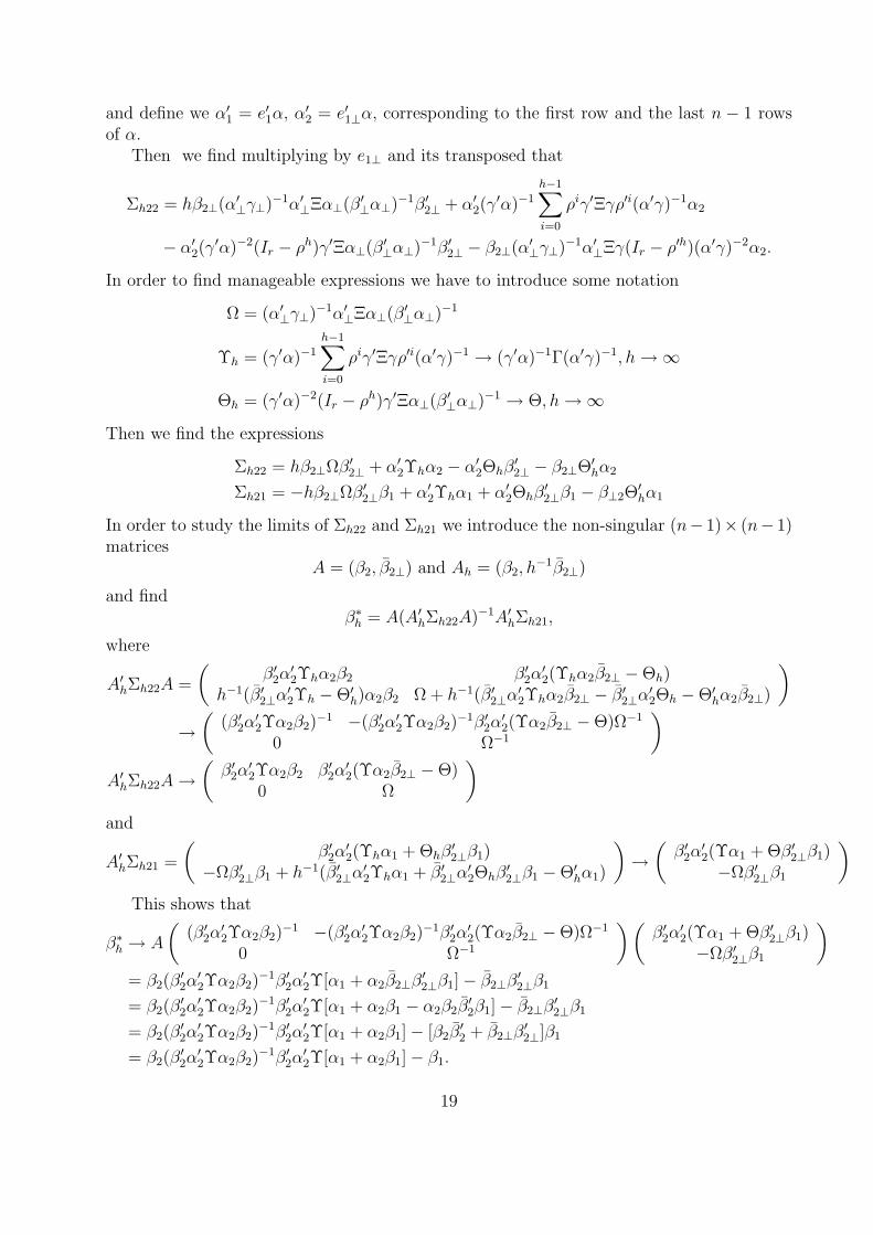
2 = e′1⊥α, corresponding to the first row and the last n − 1 rowsof α.

Then we find multiplying by e1⊥ and its transposed that

Σh22 = hβ2⊥(α′⊥γ⊥)−1α′

⊥Ξα⊥(β′⊥α⊥)−1β′

2⊥ + α′2(γ

′α)−1

h−1∑i=0

ρiγ′Ξγρ′i(α′γ)−1α2

− α′2(γ

′α)−2(Ir − ρh)γ′Ξα⊥(β′⊥α⊥)−1β′

2⊥ − β2⊥(α′⊥γ⊥)−1α′

⊥Ξγ(Ir − ρ′h)(α′γ)−2α2.

In order to find manageable expressions we have to introduce some notation

Ω = (α′⊥γ⊥)−1α′

⊥Ξα⊥(β′⊥α⊥)−1

Υh = (γ′α)−1

h−1∑i=0

ρiγ′Ξγρ′i(α′γ)−1 → (γ′α)−1Γ(α′γ)−1, h → ∞

Θh = (γ′α)−2(Ir − ρh)γ′Ξα⊥(β′⊥α⊥)−1 → Θ, h → ∞

Then we find the expressions

Σh22 = hβ2⊥Ωβ′2⊥ + α′

2Υhα2 − α′2Θhβ

′2⊥ − β2⊥Θ′

hα2

Σh21 = −hβ2⊥Ωβ′2⊥β1 + α′

2Υhα1 + α′2Θhβ

′2⊥β1 − β⊥2Θ

′hα1

In order to study the limits of Σh22 and Σh21 we introduce the non-singular (n− 1)× (n− 1)matrices

A = (β2, β̄2⊥) and Ah = (β2, h−1β̄2⊥)

and findβ∗

h = A(A′hΣh22A)−1A′

hΣh21,

where

A′hΣh22A =

(β′

2α′2Υhα2β2 β′

2α′2(Υhα2β̄2⊥ − Θh)

h−1(β̄′2⊥α′

2Υh − Θ′h)α2β2 Ω + h−1(β̄′

2⊥α′2Υhα2β̄2⊥ − β̄′

2⊥α′2Θh − Θ′

hα2β̄2⊥)

)→

((β′

2α′2Υα2β2)

−1 −(β′2α

′2Υα2β2)

−1β′2α

′2(Υα2β̄2⊥ − Θ)Ω−1

0 Ω−1

)A′

hΣh22A →(

β′2α

′2Υα2β2 β′

2α′2(Υα2β̄2⊥ − Θ)

0 Ω

)and

A′hΣh21 =

(β′

2α′2(Υhα1 + Θhβ

′2⊥β1)

−Ωβ′2⊥β1 + h−1(β̄′

2⊥α′2Υhα1 + β̄′

2⊥α′2Θhβ

′2⊥β1 − Θ′

hα1)

)→

(β′

2α′2(Υα1 + Θβ′

2⊥β1)−Ωβ′

2⊥β1

)This shows that

β∗h → A

((β′

2α′2Υα2β2)

−1 −(β′2α

′2Υα2β2)

−1β′2α

′2(Υα2β̄2⊥ − Θ)Ω−1

0 Ω−1

)(β′

2α′2(Υα1 + Θβ′

2⊥β1)−Ωβ′

2⊥β1

)= β2(β

′2α

′2Υα2β2)

−1β′2α

′2Υ[α1 + α2β̄2⊥β′

2⊥β1] − β̄2⊥β′2⊥β1

= β2(β′2α

′2Υα2β2)

−1β′2α

′2Υ[α1 + α2β1 − α2β2β̄

′2β1] − β̄2⊥β′

2⊥β1

= β2(β′2α

′2Υα2β2)

−1β′2α

′2Υ[α1 + α2β1] − [β2β̄

′2 + β̄2⊥β′

2⊥]β1

= β2(β′2α

′2Υα2β2)

−1β′2α

′2Υ[α1 + α2β1] − β1.

19

We now find from β2 = e′1⊥γ2 and α′2 = e′1⊥α that

β′2α

′2 = γ′

2e1⊥e′1⊥α = e′1⊥γ′α

α1 + α2β1 = α′(e1 + e1⊥e′1γ1) = α′γ1 = α′γe1.

Hence

β′2α

′2Υα2β2 = e′1⊥γ′α(γ′α)−1Γ(α′γ)−1α′γe1⊥ = Γ22

β′2α

′2Υ[α1 + α2β1] = e′1⊥Γ(α′γ)−1[α1 + α2β1] = Γ21,

and therefore

β∗h → β2Γ

−122 e′1⊥Γ(α′γ)−1[α1 + α2β1] − β1 = −β1 + β2Γ

−122 Γ21 = β∗

coint

as was to be proved.

20

10 20 30 40 50 60 70 80 90 1000.8

1

1.2

1.4

1.6

1.8

2

2.2

h

β h

Correlation hedge βCorr

Cointegration hedge β

Optimal hedge βh*

Figure 1: Optimal hedge coefficient β⋆h under limited mean reversion and high covariance.

21

10 20 30 40 50 60 70 80 90 100

0.5

1

1.5

2

2.5

3

3.5

4

4.5Portfolio volatility for different hedge types

h

Vol

atili

ty

Correlation hedge portfolio volatility

Cointegration hedge portfolio volatility

Optimal hedge portfolio volatility

Figure 2: Volatility of various portfolios under limited mean reversion and high covariancefor the correlation hedge βCorr (thick line), the cointegration hedge β (thin line) and for theoptimal hedge β⋆

h (dotted line) for different holding periods.

22