Optimal Fiscal Policy in Overlapping GenerationsModels∗

Carlos GarrigaFlorida State University and CREB

January 2001(First version: December 1998)

Abstract

This paper provides, from a theoretical and quantitative point of view, an explanationof why taxes on capital returns are high by analyzing the optimal Þscal policy in an econ-omy with intergenerational redistribution. For this purpose, the government is modeledexplicitly and can choose (and commit to) an optimal tax policy in order to maximizesociety�s welfare. In an inÞnitely lived economy with heterogeneous agents, the long runoptimal capital tax is zero. If heterogeneity is due to the existence of overlapping gener-ations, this result in general is no longer true. I provide a sufficient conditions for zerocapital, and show that a general class of preferences, commonly used in the macro andpublic Þnance literature, violate this condition. For a version of the model, calibrated tothe US economy, the main results are: Þrst, if the government is restricted to use pro-portional taxes across generations, the model can account for the observed capital andlabor income taxes. Second, if the government can use speciÞc taxes for each generation,then the age proÞle capital tax pattern implies subsidizing asset returns of the youngergenerations and taxing at higher rates the asset returns of the older ones.

Keywords: Optimal taxation.J.E.L. classiÞcation codes: E62, H21.

∗I want to thank the useful comments of Pat Kehoe, Juan Carlos Conesa, Antonio Manresa,Begoña Dominguez, Tim Kehoe, Tim Salmon, Jim Cobbe and seminar participants at the 2000Meeting of the Society for Economic Dynamics, the Federal Reserve Bank of Minneapolis, Uni-versity of Texas-Austin and Universidad Carlos III de Madrid. I also acknowledge the Þnancialsupport of DGCYT PB96-0988 from Ministerio de Educación y Cultura and SGR97-180 from theGeneralitat de Catalunya. Correspondence: Departament of Economics, Florida State Univer-sity, 246 Bellamy, Tallahassee, Florida 32306-2180 (USA). E-mail: cgarriga@garnet.acns.fsu.edu

1

1 Introduction

The standard view of economists is that capital returns should not be taxed at all.In Lucas� words: �I believed that the single most desirable change in the U.S. taxstructure would be the taxation of capital gains as ordinary income. I now believethat neither capital gains nor any source of income from capital should be taxedat all. My earlier view was based on what I viewed as the best available economicanalysis, but of course I think my current view is based on a better economicanalysis�, (Lucas (1990)).

This view is built on a well-established theory of optimal Þscal policy. Instandard neoclassical growth models, with inÞnitely-lived consumers, the optimalpolicy predicts that capital taxes should be zero in the long run and importantwelfare gains can be realized by implementing this policy. This result was Þrstshown by Chamley (1986). Several papers have extended this result to more com-plex economies that include heterogeneous consumers (Judd (1985)), endogenousgrowth (Jones, Manuelli and Rossi (1997)), aggregate shocks (Chari, Christianoand Kehoe (1994)), and open economies (Razin and Sandka (1995)). In each casethe result is the same, capital returns should not be taxed at all.

However the observed data for most OECD economies show that capital taxesare different from zero. For instance in the US the average capital tax over theperiod 1965−1995 is around 35%, and in the U.K and Germany it is around 37%and 23.5% respectively.

At this point theory and data seem to be mutually exclusive. Why mightgovernments choose to tax capital returns at high rates? Can we Þnd a modelwhere the optimal policy implies capital taxes different from zero? Is this modelconsistent with the observed capital taxation?

The main contribution of this paper is to show that when we consider a Þnitelifetime economy, in the tradition of Auerbach and Kotlikoff (1987), for the classof utility functions commonly used in the macro and public Þnance literature theoptimal policy implies a tax rate on capital returns different from zero. Moreover,for some plausible choices of parameter values the optimal policy is consistentwith the average capital taxes observed for most OECD countries.

This result contrasts with previous results in the extensive literature on op-timal Þscal policy in overlapping generations economies, for example Pestieau(1974), Atkinson and Sandmo (1980), Atkinson and Stiglitz (1980), and more re-cently Chari and Kehoe (1999). These papers focus their analysis on the steadystate and Þnd restrictive conditions for zero capital taxes in the long run. Theseconditions cannot be extended to economies where agents live more than twoperiods.

This result together with the standard results in inÞnite-lived consumers mod-els suggested other explanations to account for the observed high capital taxation:incomplete markets (Aiyagari (1995) and Domeij and Heathcote (2000)), timeconsistency issues (Klein and Rios-Rull (2000) and Phelan and Stachetti (2001)),or information problems (Golosov, Kocherlakota and Tsyvinski (2001)). One ofthe main problems in these papers is that Þscal policy plays two roles: Þnance

2

government expenditure and substitute for missing markets (insurance, lack ofcommitment or information problems). This raises the question why the govern-ment cannot implement some other type of policy to achieve this goal, and setcapital taxes to zero. In this paper markets are complete, and the focus is on thedistortions due to taxation.

This paper provides theoretical foundations as well as quantitative results forthe optimal Þscal policy in Þnite lifetime environments. The main theoreticalresult is that the optimal tax on capital returns is in general different from zero,both in the transition path and in the long run. I provide a sufficient conditionfor the zero capital tax result and show that a general class of preferences violatesthis condition.

To provide some intuition it is useful to compare this result with the optimalpolicy in an inÞnitely-lived consumers economy. In a dynamic economy there iscertain equivalence between tax instruments. For example, a tax system thatuses positive capital taxes to Þnance government expenditure is equivalent to atax system that uses an ever-increasing consumption tax and an increasing laborsubsidy. In an inÞnitely-lived consumer economy, if preferences are separable andexhibit some degree of substitutability, an increasing consumption tax creates animportant distortion on the relative price between today�s consumption and con-sumption at period T . Then given that individuals want to smooth consumption,they prefer a constant consumption tax than an ever-increasing consumption tax.

In contrast, if individuals live a Þnite number of periods, as in an overlap-ping generations model, the distortions associated with this policy are not thatimportant because for a given generation today�s consumption and period T con-sumption are not perfectly substitutable. Hence the effect of capital distortions ismuch smaller and not necessarily bigger than distortions caused by other taxes.

In general taxes on capital returns are different from zero unless we make someassumption either on the lifetime horizon or on the set of instruments available tothe government. The optimal capital tax can be zero if we consider either a twoperiod OG model where the old generation does not supply labor (this is the stan-dard framework used in the referenced literature1), or the government is allowedto use age-dependent taxes. In these two cases the uniform tax property ensureszero capital taxes, both in the transition path and in the long run. Restrictionson the set of tax instruments that the government can use play an importantrole in the determination of the optimal policy. This point is emphasized in thequantitative results.

For a version of the model calibrated to the US economy the key Þndings are:Þrst, if the government uses proportional taxes across ages, the optimal capital taxis as high as in the US economy. Second, if the government can use age-dependent

1In a simple two period model, where only the young generations supply labor, the standardassumption for the set of Þscal instruments available implies that labor income tax affects younggenerations while capital taxes affect old generations in the economy. Therefore, under certainassumptions on the utility function (satisfy unitary expenditure elasticity), it can be shown thatcumulative distortions of the capital income taxes on the intertemporal decisions make younggenerations prefer a static distortion due to labor taxes. If we allow generations to work in allperiods, then the previous result is no longer true even with the same type of preferences.

3

proportional taxes, then the age proÞle capital tax pattern implies a subsidy onthe asset returns of the younger generations and a tax on the asset holdings ofthe older ones. Hence, constraints on the set of instruments that the governmentcan use are quantitatively too important to be ignored.

At this point two papers deserve special comments. Escolano (1992) showed,using a quantitative analysis, that in overlapping generations economies, positivecapital taxes can be optimal and the efficiency loss of the current Þscal systemin the US economy is not quantitatively relevant. In his model for a particularvalue of the government discount factor, the optimal tax on capital returns is zero.This paper has two shortcomings, Þrst it does not derive sufficient conditions tocheck whether this is a general result or not. Second, the quantitative exerciseimplies that the government only has access to proportional taxes across ages.Independent work by Erosa and Gervais (2000) considers a similar economy andderives some of the results presented here for the case of age-dependent taxes.

The paper is organized as follows. Section 2 describes the environment anddeÞnes a competitive equilibrium, and section 3 deÞnes the government problemand derives sufficient conditions for the zero capital tax result. Section 4 describesthe calibration process and the main quantitative Þndings under different taxarrangements. Finally, section 5 concludes.

2 The economy

The model is a standard overlapping generations production economy with twogoods, a consumption-capital good and labor. Agents live I ≥ 2 periods andeach cohort is populated by a continuum of identical households, represented bythe interval [0, 1]. Without loss of generality, the population is assumed to bestationary and its total size is constant.2

There is a representative Þrm that produces aggregate output Yt using aconstant returns to scale production function F (Kt, Lt), using aggregate cap-ital Kt and aggregate labor Lt as primary inputs. Labor is measured in ef-Þciency units. The production function F : R2

+ → R+ is strictly concave,monotone, homogeneous of degree one and continuously differentiable, with par-tial derivatives F1(Kt, Lt) > 0 and F2(Kt, Lt) > 0. Furthermore for all K,L ∈ R2

+

F (0, L) = F (K, 0) = 0. Capital depreciates each period at a constant rateδ ∈ (0, 1) and there is no exogenous technological change. These assumptionsimply that in competitive factor markets Þrms will make zero proÞts, hence it isunnecessary to specify Þrms� ownership. Then, each period prices are determinedby the marginal products, that is

rt = F1(Kt, Lt)− δ, (1)

wt = F2(Kt, Lt), (2)

where rt denotes the interest rate net of depreciation and wt is the wage rate perefficiency unit of labor. Let Ct and Lt denote aggregate consumption and labor

2This is not an important assumption for the basic results and simpliÞes notation.

4

respectivelyCt =

XI

i=1cit ∀t, (3)

Lt =XI

i=1²i`it ∀t, (4)

where cit denotes consumption of an individual of age i at time t, ²i denote her

efficiency units, and `it is hours worked.The government in this economy Þnances an exogenous sequence of expendi-

ture {G}∞t=0 using proportional capital taxes θt, labor taxes τ t and debt Dt. Thegovernment intertemporal budget constraint is

Gt +RtDt ≤ τ twtLt + θtrtKt +Dt+1 ∀t, (5)

where Rt denotes the return on government debt.3 Let π = {τ `t , θt}∞t=0 be a taxpolicy consisting of an inÞnite sequence of proportional taxes. Notice that thegovernment debt has not been included as part of the policy. Given the initialgovernment debt D0 and the sequence {G}∞t=0, we can back up the sequence ofdebt {D}∞t=1.

The economy resource constraint at each time t is given by

Ct +Kt+1 − (1− δ)Kt +Gt ≤ F (Kt, Lt) ∀t. (6)

Households in this economy have standard preferences deÞned over a stream ofconsumption and labor {cit, `it}∞t=0, and are represented by a time separable utilityfunction XI

i=1βi−1U(cit, `

it) ∀t, (7)

where β > 0 is the subjective discount factor. The utility function U : R2+ → R+

is C2, strictly concave, increasing in consumption Uc(cit, `it) > 0, decreasing in

labor U`(cit, `it) < 0. The agents are endowed at each period with a time invariant

vector of efficiency units of labor ² = (²1, ..., ²I). One unit of time of an individualof age i can be transformed into ²i units of input in the production function. Ateach period, taking prices and taxes as given, individuals choose consumption,labor supply, and asset holdings. Households� decisions face a sequence of budgetand non-negativity constraints:

cit + ai+1t+1 ≤ (1− τ t)wt²i`it + (1 + rt(1− θt))ait 1 ≤ i ≤ I ∀t, (8)

a1t = 0, 0 ≤ `it ≤ 1, cit ≥ 0 ∀t.

Households are born with zero assets and accumulate wealth ai+1t+1 in three forms:

buying government debt of one period maturity and lending to households orÞrms. Government debt and capital are perfect substitutes for the individualinvestment decisions.

3Without loss of generality I have abstracted from consumption taxes, because in this modelthey are redundant.

5

At the initial period, t = 0, the stock of capital and debt is distributed amongthe initial, s, generations (individuals of age 2 to I). Let as0 be the initial endow-ment of wealth of generation s. The period 0 budget constraint is given by

cs0 + as+11 ≤ (1− τ0)w0²

s`s0 + (1 + r0(1− θ0))as0 2 ≤ s ≤ I, (9)

Intertemporal trade between generations to smooth consumption over the life-cycle is allowed. 4 Market clearing conditions in the capital markets imply:

Kt+1 =XI

i=1ait+1 −Dt+1 ∀t, (10)

Next we proceed by deÞning the notion of competitive equilibrium.

DeÞnition 1 (Competitive Equilibrium): Given a tax policy π and a se-quence of government expenditure {Gt}∞t=0, a competitive equilibrium in this econ-omy is a sequence of individual allocations {{cit, `it, ait+1}Ii=1}∞t=0, production plans{Kt, Lt}∞t=0, government debt {Dt+1}∞t=0, and relative prices {rt, wt, Rt}∞t=0, suchthat:

1. Consumers born at time t ≥ 1 maximize (7) subject to (8). Similarly consumersborn at t ≤ 0 maximize utility subject to (9).2. In the production sector (1) and (2) are satisÞed for all t.

3. Factor markets clear and (4) and (10) hold.

4. The government budget constraint (5) is satisÞed.

5. Feasibility (6) is satisÞed for all t.

3 Government problem

Let�s consider the policy problem faced by the government. Suppose that thereexists a benevolent government that chooses the optimal policy π∗, to maximizethe welfare of all (present and future) generations subject to given constraints.These constraints imply that the present value government budget constraint mustbe satisÞed and the allocation associated with the optimal policy has to belongto the subset of policies for which a competitive equilibrium exists.

The optimal Þscal policy might cause time-consistency problems because thegovernment might have incentives to deviate from the optimal policy once it hasbeen announced and taken into account by the agents. This time-consistencyissue has been shown in Kydland and Prescott (1977) and Calvo (1978). In thispaper we abstract from these issues and it is assumed that the government can

4This assumption implies that credit markets are complete, in the sense that agents are notcredit constrained. Aiyagari (1995) shows that in an economy with incomplete markets theoptimal capital tax is positive. The basic intuition works as follows. Because of the incom-plete insurance markets, there is a precautionary motive for accumulating capital. In addition,the possibility of being borrowing constrained in the future leads to some additional savings.These facts increase the capital stock. Then, a positive capital tax is needed to reduce capitalaccumulation and equalize the interest rate of the economy to the rate of time preference.

6

commit to future policies. This commitment technology is modelled in the timingof the decisions and it works as follows: Þrst the government chooses a policy πat time zero, second agents choose optimal allocations taking as given the policyand prices.5

The government is benevolent and values all present and future generationsin the economy. The government objective function is deÞned as a weighted sumof each generation�s lifetime utility6. Therefore the government assigns a non-negative weight to all individuals when born. Let ωt ∈ R+ be the relative weightof a generation born at time t. The sequence of weights {ωt}∞t=−(I−1) is boundedabove by a large positive constant Γ < ∞. Formally the government objectivefunction is

W ({cit, lit}) =X∞

t=0

XI

i=1ωt+1−i

³βi−1U(cit, l

it)´. (11)

To Þnd an asymptotic steady state for the government problem it is convenientto impose some structure on the sequence of weights7, such as

limt→∞

ωtωt+1

=1

λ> 1.

where λ can be view as a subjective valuation of present and future generations.If the government valuation of future generations is high, then λ is close to one.

The government problem of choosing the optimal policy is solved using theso-called primal approach, as in Lucas and Stokey (1983) and Chari and Ke-hoe (1999). One way to think of it is having the government choosing directlyfrom the set of implementable allocations given a tax policy π. Then from theallocations it is possible to back out policies and prices from the competitiveequilibrium. The set of implementable allocations is characterized by the periodresource constraint and an implementability constraint for each generation. Theimplementability constraint takes into account that changes in the policy willaffect agents� decisions, therefore prices and government revenues. These con-straints are constructed by substituting the households� budget constraints, andÞrms� Þrst-order conditions, into the households� decision rules. The next propo-sition shows how to characterize the set of implementable allocations for a givenclass of policy π.

Proposition 1 (Set of Implementable Allocations): Given a tax policy π anycompetitive equilibrium allocation x = {{cit, lit}Ii=1,Kt+1}∞t=0 satisÞes the periodresource constraint:XI

i=1cit +Kt+1 − (1− δ)Kt +Gt = F (Kt,

XI

i=1²i`it) ∀t, (12)

5If a commitment technology is not available there are two ways to go, one is to Þnd mecha-nisms that substitute for commitment as in Chari and Kehoe (1990) or Stokey (1991), or solve thecase where neither commitment or reputation mechanism are operative as in Klein and Ríos-Rull(1999) or Phelan and Stacchetti (1999).

6In the early literature, see Samuelson (1958) or Diamond (1965), society�s welfare was rep-resented by the utility of a representative generation in steady state.

7Atkinson and Sandmo (1980) derive, using the so-called dual approach, the optimal capitaltax in the steady state for different government discount factors. It can be easily shown that allare particular cases of this formulation.

7

implementability constraints for all newborn generations:XI

i=1βi−1

³cit+i−1Uci

t+i−1+ `it+i−1U`it+i−1

´= 0 t ≥ 0, (13)

implementability constraints for the initial old generations at t = 0:XI

i=sβi−s

³cii−sUci

i−s+ `ii−sU`ii−s

´= Ucs

0as0 s = 2, ..., I, (14)

marginal rates of substitution between consumption and labor, and consumptiontoday and tomorrow are equal across consumers:

Uc1t

Ul1t²1 = . . . =

UcIt

UlIt²I ∀t, i, (15)

Uc1t

Uc2t+1

= . . . =UcI−1

t

UcIt+1

∀t, i. (16)

Furthermore, given allocations that satisÞes (12), (13), (14), (15), and (16), wecan construct a tax policy π = {τ t, θt}∞t=0, a sequence of government debt {Dt}∞t=0

and relative prices {rt, wt, Rt}∞t=0, that together with the allocation x, constitutea competitive equilibrium.

Proof. We Þrst proceed by showing that the allocations in a competitive equilib-rium must satisfy (12), (13), (14), (15), and (16). Condition (12) is straightforwardfrom substituting the labor market clearing condition (4) into (6). To derive theimplementability constraint for each generation we have to use the Þrst-orderconditions of the consumer�s problem

βiUcit= αit ∀t, i, (17)

βiUlit= −αit(1− τ t)wt²i ∀t, i, (18)

αit = αi+1t+1 [1 + rt+1(1− θt+1)] ∀t, i, (19)

where αit denotes the Lagrange multiplier of age i budget constraint. To derivethe implementability constraint we have to multiply (17), (18) by their respectivecontrol variables and then add them up for all i. Then substituting in the re-sulting expression the households� budget constraint and using (19) we derive theimplementability constraint for the newborn generations (13). For the initial gen-erations in the economy at time t = 0 the distribution of asset holdings appearson the right hand side of (14).

If the government is restricted to use the same proportional taxes for all gen-erations the set of implementable allocations needs to include constraints (15),and (16).

Now we prove the second part of Proposition 1. From the aggregate capitalstock, Kt, and the aggregate labor supply, Lt, we construct the relative pricesusing the Þrm�s Þrst-order conditions (1) and (2).

8

To derive the policy π = {τ t, θt}∞t=0 we substitute the allocations {{cit, lit}Ii=1}∞t=0

and the equilibrium prices {rt, wt, }∞t=0 into households� Þrst-order conditions asfollows

1− τ t = −Ulit

Ucit²iFLt

∀t, i, (20)

1− θt+1 =1

FKt − δ

Ucit

βUci+1t+1

− 1 ∀t, i. (21)

The tax rates are set to satisfy the consumers� Þrst-order conditions. The returnon debt holdings for all t is determined by an arbitrage argument, Rt = 1 +rt(1 − θt). Substituting Uci

tand U`it from the consumers problem into (13), (14)

we obtain the intertemporal budget constraint of each household (for simplicitywritten in Arrow-Debreu terms):XI−1

i=0pt+i

hcit+i − (1− τ t+i)wt+i²i`it+i

i= 0 ∀i. (22)

The sequence of government debt {Dt}∞t=0 is adjusted to satisfy the desiredcapital-output ratio, and is obtained using market clearing in the capital market

Dt+1 =XI

i=1ait+1 −Kt+1. (23)

This expression does not impose any restrictions on the sign of the governmentdebt, therefore it might be negative. If feasibility and the households budgetconstraint are satisÞed, then the government budget constraint is also satisÞed.

It is important to note that if an allocation x = {{cit, lit}Ii=1,Kt+1}∞t=0 satis-Þes feasibility and each generation�s implementability constraint, that does notimply that the marginal rates of substitution across consumers are equal. Tosee this, suppose that the government can use age-dependent taxes, that is πi ={{τ it, θit}Ii=1}∞t=0, then if an allocation x satisÞes feasibility and the implementabil-ity constraint, the marginal rates of substitution do not need to be equal acrossgenerations at a given point in time. The constraints in the set of taxes that thegovernment can use will play an important role to determine the optimal Þscalpolicy but are often not considered.

In a representative agent economy, the government has incentives to tax heav-ily the initial stock of capital. To avoid this problem it is commonly assumed thatthe government takes as given the initial capital tax. In this type of economy thegovernment faces an inÞnite sequence of implementability constraints, becausethe economy is populated over time by an inÞnite number of individual that livea Þnite number of periods. Then, taxing the initial distribution of asset holdings{as0}Is=0 is equivalent to tax an inelastically supplied factor and has intergenera-tional redistributive effects, therefore it is assumed that the government takes asgiven the initial capital tax {θ0}. Dropping this assumption does not affect themain results of the paper because capital taxes at t = 0 cannot be used to mimiclump-sum taxes beyond t = 1.

9

The government�s optimal taxation problem is to choose x from the set of im-plementable allocations such that the utilitarian objective function is maximized.Formally the Ramsey allocation problem is,

max{{ci

t,`it}I

i=1,Kt+1}∞t=0

X∞t=0

XI

i=1ωt+1−i

hβi−1U(cit, `

it)i, (24)

s.t.XI

i=1cit +Kt+1 − (1− δ)Kt +Gt = F (Kt,

XI

i=1²i`it) ∀t, (25)XI

i=1βi−1

³cit+i−1Uci

t+i−1+ `it+i−1U`it+i−1

´= 0 t ≥ 0, (26)XI

i=sβi−s

³cii−sUci

i−s+ `ii−sU`ii−s

´= Ucs

0as0 s = 2, ..., I, (27)

Ucit

Uci+1t+1

= ... =UcI−1

t

UcIt+1

∀t, i = 1, ..., I, (28)

Uc1t

U`1t²1 = ... =

UcIt

U`It²I ∀t, i = 1, ..., I. (29)

where the initial distribution of wealth as,0, K0 = K > 0 and {Gt}∞t=0 are givenand cit ≥ 0, `it ∈ (0, 1).

The allocation x that solves the Ramsey allocation problem is constrainedefficient, in the sense that there exists no other constrained efficient allocation x0

that Pareto dominates the optimal.To solve the government problem I follow a particular approach assuming that

the government has access to a complete set of age-dependent taxes (that is drop-ping the additional constraints on the marginal rates of substitution), and thenverify under what conditions capital taxes will be zero. If capital taxes are notzero in the less constrained problem, then we cannot expect them to be zero forthe age-independent tax case. Then, it is useful to redeÞne the objective functionby introducing the implementability constraint on it, and use the associated La-grange multiplier as co-state variable. Let ηt−i be the Lagrange multiplier of theimplementability constraint for the agent born in period t− i. Let�s deÞne

V (cit, `it, ηt−i) = U(c

it, `

it) + ηt−i(c

itUci

t+ `itU`it). (30)

The modiÞed Ramsey Allocation Problem can be written as follows:

max{{ci

t,`it}I

i=1,Kt+1}∞t=0

X∞t=0

XI

i=1ωt+1−i

hβi−1V (cit, `

it, ηt−i)

i−XI

s=2η1−sUcs

0as0,

(31)s.t.

XI

i=1cit +Kt+1 − (1− δ)Kt +Gt = F (Kt,

XI

i=1²i`it) ∀t. (32)

This problem has a similar structure to an optimal planning problem, exceptthat the period utility function U(·) has been replaced by a �pseudo� utility func-tion V (·). If the government has access to lump-sum taxes, the implementabilityconstraint will not be binding, ηt−i = 0, and it will not be optimal to use distor-tionary taxes and the economy would achieve a full efficient allocation. Let µt be

10

the Lagrange multiplier of the resource constraint, then the Þrst-order necessaryconditions at t > 0 are deÞned by

[cit] ωt+1−iβi−1Vcit− µt = 0,

[ci+1t ] ωt−iβiVci+1

t− µt = 0,

[`it] ωt+1−iβi−1V`it+ µtFLt²

i = 0,

[Kt+1] −µt + µt+1(1− δ + FKt) = 0,

together with the transversality condition for the optimal capital path:

limt→∞µtKt+1 = 0. (33)

Throughout the paper I assume that the solution of the Ramsey allocation prob-lem exists and that the time paths of the solutions converge to a steady state.Neither of these assumptions is innocuous. Notice that since the set of alloca-tions that satisfy the implementability constraint might fail to be convex, theÞrst-order conditions are necessary but not sufficient (for a detailed discussion ofnonconvexities, see Lucas and Stokey (1983)). Rearranging terms, we have:

ωt+1−iVcit= ωt+2−iVci

t+1(1− δ + FKt+1) ∀i, t, (34)

V`itVci

t

= −FLt²i ∀i, t, (35)

Vcit=

ωt−iωt+1−i

βVci+1t, ∀i, t. (36)

Notice that Equation (34) is slightly different from the competitive equilib-rium Euler equation. In this case the government equates the derivative of theobjective function of a newborn generation at different times. Equation (35) isthe intratemporal condition between consumption and labor, that determines theamount of effective hours worked by each generation at a given period t. Finally,equation (36) is the static redistributive condition, and implies that the govern-ment will assign consumption among two different generations according to theratio of their relative weights.

For the initial s generations at t = 0, the Þrst-order necessary conditions aredifferent from the previous ones, given the initial distribution of asset holdings.The Þrst-order condition with respect to consumption-labor is given by

V`s0 − η1−shUcs

0`s0((1 + FK0(1− θs0)as0) + Ucs

0FK0`s0

(1− θs0)as0i

Vcs0− η1−sUcs

0cs0((1 + FK0(1− θs0)as0)

= −FL0²s, (37)

and the redistributive Þrst-order condition is

Vcs0− η1−sUcs

0cs0((1 + FK0(1− θs0)as0)

Vcs+10− η2−sUcs+1

0 cs+10

³(1 + FK0(1− θs+1,t)a

s+10

´ = βωs+1

ωs. (38)

11

This redistributive condition does not appear in the competitive equilibriumÞrst-order conditions, but it is very useful to derive the optimal capital taxes.Updating (36) one period and substituting in (34) we obtain

Vcit= βVci+1

t+1(1− δ + FKt+1) ∀i, t, (39)

This new expression is very similar to a life-cycle Euler equation, but instead ofhaving the marginal utility with respect to consumption it has the derivative ofV (·).

To derive the optimal tax policy π∗ we combine the Þrst-order conditions of theRamsey Allocation Problem together with the competitive equilibrium Þrst-orderconditions. The resulting expression is the optimal capital tax rate

θ∗t+1 =1

βrt+1

Vcit

Vci+1t+1

−Uci

t

Uci+1t+1

∀i, t. (40)

We use the same procedure to determine the expression for the optimal labortax rate

τ∗t = 1−Uci

t

U`it

V`itVci

t

∀i, t. (41)

It is important to remark that we are solving a relaxed version of the Ramseyproblem, hence we cannot expect that taxes on capital returns are zero unlesstwo conditions are satisÞed: Þrst, the ratio Vci

t/Vci+1

t+1is equal to the solution

of the competitive equilibrium Ucit/Uci+1

t+1, and second, the additional constraints

on marginal utilities are also satisÞed. Hence in these type of economies theoptimal capital tax is affected by the distortions in the labor market implied bythe restrictions on the set of taxes π.

If we drop the age subscripts from the Þrst-order conditions of the Ramseyproblem, the associated expression for the optimal tax policy is equal to theone obtained in an inÞnite-lived consumer economy. Chamley (1986) proves twoimportant results. First, for a general class of utility functions capital taxes shouldbe zero in the long run (consumption is constant, therefore Uct = Uct+1). Second,for a particular class of functions, that satisfy Vct/Vct+1 = Uct/Uct+1 , the optimalcapital income taxes are zero after a Þnite number of periods. The conditions forthe zero capital result in the transition path are generally viewed as an applicationof the uniform commodity taxation principle (see Atkinson and Stiglitz (1980)),that speciÞes conditions under which taxing all goods at the same rate is optimal.

In overlapping generations economies the previous results are not generallytrue. The next proposition provides sufficient conditions that preferences need tosatisfy for the zero capital income tax result.

Proposition 2: If the government has access to proportional distortionary taxesacross agents, then taxes on capital income are zero for t ≥ 2 if preferences satisfy:

θt = 0⇒citUcci

t+ `itU`ci

t

Ucit

=`itU``it + c

itUc`it

U`it∀t > 1 (42)

12

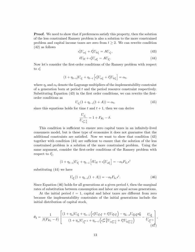
Proof. We need to show that if preferences satisfy this property, then the solutionof the less constrained Ramsey problem is also a solution to the more constrainedproblem and capital income taxes are zero from t ≥ 2. We can rewrite condition(42) as follows

citUccit+ `itU`ci

t= AUci

t, (43)

`U`` + citUc`it

= AU`it . (44)

Now let�s consider the Þrst-order conditions of the Ramsey problem with respectto cit

(1 + ηt−i)Ucit+ ηt−i

hcitUcci

t+ `itU`ci

t

i= αt,

where ηt and αt denote the Lagrange multipliers of the implementability constraintof a generation born at period t and the period resource constraint respectively.Substituting Equation (43) in the Þrst order conditions, we can rewrite the Þrst-order conditions as

Ucit(1 + ηt−i(1 +A)) = αt, (45)

since this equations holds for time t and t+ 1, then we can derive

Ucit

Uci+1t+1

= 1 + FKt − δ.

This condition is sufficient to ensure zero capital taxes in an inÞnitely-livedconsumers model, but is these type of economies it does not guarantee that theadditional constraints are satisÞed. Now we want to show that condition (43)together with condition (44) are sufficient to ensure that the solution of the lessconstrained problem is a solution of the more constrained problem. Using thesame argument, consider the Þrst-order conditions of the Ramsey problem withrespect to `it,

(1 + ηt−i)U`it + ηt−ih`U`` + c

itUc`it

i= −αtFLt²

i

substituting (44) we have

U`it(1 + ηt−i(1 +A)) = −αtFLt²

i. (46)

Since Equation (46) holds for all generations at a given period t, then the marginalrates of substitution between consumption and labor are equal across generations.

At the initial period t = 1, capital and labor taxes are different from zerobecause the implementability constraints of the initial generations include theinitial distribution of capital stock,

θ1 =1

β(FK1 − δ)

(1 + ηs)Ucs0+ ηs−i

³cstUcs

t cst+ `stU`st cs

t

´− η1−sUcs

0cs0as0

(1 + ηs)Ucs+11+ ηs−i

³cs+1t+1Uccs+1

t+1+ `stU`cs+1

t+1

´ − Ucs0

Ucs+11

,(47)

13

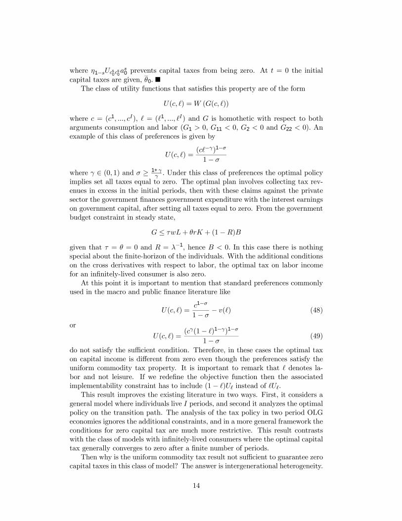
where η1−sUcs0c

s0as0 prevents capital taxes from being zero. At t = 0 the initial

capital taxes are given, θ0.The class of utility functions that satisÞes this property are of the form

U(c, `) =W (G(c, `))

where c = (c1, ..., cI), ` = (`1, ..., `I) and G is homothetic with respect to botharguments consumption and labor (G1 > 0, G11 < 0, G2 < 0 and G22 < 0). Anexample of this class of preferences is given by

U(c, `) =(c`−γ)1−σ

1− σwhere γ ∈ (0, 1) and σ ≥ 1+γ

γ . Under this class of preferences the optimal policyimplies set all taxes equal to zero. The optimal plan involves collecting tax rev-enues in excess in the initial periods, then with these claims against the privatesector the government Þnances government expenditure with the interest earningson government capital, after setting all taxes equal to zero. From the governmentbudget constraint in steady state,

G ≤ τwL+ θrK + (1−R)Bgiven that τ = θ = 0 and R = λ−1, hence B < 0. In this case there is nothingspecial about the Þnite-horizon of the individuals. With the additional conditionson the cross derivatives with respect to labor, the optimal tax on labor incomefor an inÞnitely-lived consumer is also zero.

At this point it is important to mention that standard preferences commonlyused in the macro and public Þnance literature like

U(c, `) =c1−σ

1− σ − v(`) (48)

or

U(c, `) =(cγ(1− `)1−γ)1−σ

1− σ (49)

do not satisfy the sufficient condition. Therefore, in these cases the optimal taxon capital income is different from zero even though the preferences satisfy theuniform commodity tax property. It is important to remark that ` denotes la-bor and not leisure. If we redeÞne the objective function then the associatedimplementability constraint has to include (1− `)U` instead of `U`.

This result improves the existing literature in two ways. First, it considers ageneral model where individuals live I periods, and second it analyzes the optimalpolicy on the transition path. The analysis of the tax policy in two period OLGeconomies ignores the additional constraints, and in a more general framework theconditions for zero capital tax are much more restrictive. This result contrastswith the class of models with inÞnitely-lived consumers where the optimal capitaltax generally converges to zero after a Þnite number of periods.

Then why is the uniform commodity tax result not sufficient to guarantee zerocapital taxes in this class of model? The answer is intergenerational heterogeneity.

14

This factor plays an important role in this result, because the government facesadditional constraints if taxes have to be equal across generations at each periodt, (i.e. marginal rates of substitution need to be equal across consumers). Inthis case the solution of the less constrained problem is not a solution to themore constrained problem. This is not true in an economy with heterogeneousinÞnitely-lived consumers. Chari and Kehoe (1999) show that the additionalconstraints are satisÞed if the production function F (·) has the form F (K,L) =F (K,H(L)), where H(·) is some function. In an overlapping generations economythis argument does not apply because the properties of the zero capital tax resultdepend on U(·) and not on F (·). In the numerical simulations it will be clear thatthese additional constraints have important quantitative effects.

In general taxes on capital returns are different from zero unless we make someassumption either on the lifetime horizon or on the set of instruments available tothe government. The next proposition states that the additional set of constraintsplay a crucial role to determine the optimal Þscal policy in this type of economies.

Proposition 3: In this environment the uniform commodity tax result is a suf-Þcient condition to ensure zero capital taxes if:

1) The government has access to age-dependent taxes, or

2) I=2 and the old generation does not supply labor.

Proof. If the government can use age-speciÞc taxes the Ramsey allocation dropsthe additional constraints, therefore the optimal policy for utility functions of theform (48) and (49) imply zero capital taxes from period two onwards. In this caselabor taxes are different from zero. Equivalently in a two period OLG economywhere the old generation does not supply labor, the government problem does notinclude additional constraints. The young generation supplies labor in the marketwhile the old generation supplies capital.

In a different environment the previous result might not be true. Considera standard two period OLG model but suppose the young generations have anendowment, mt, which is not taxed at all. This is almost equivalent to consideringan exogenously Þxed labor supply. Then, the new implementability for a newborngeneration is

c1tUc1t+ `1tU`1t + βc

2t+1Uc2

t+1= mtUc1

t

Then even if preferences satisfy the uniform commodity taxation property,the Ramsey taxes on c1t and c

2t+1 are not uniform, that implies capital taxes

different from zero. The previous example is useful because it highlights therelation between taxes on consumption and capital, and gives some of the intuitionof why it might be optimal to tax capital. In an overlapping generations model,the distortions associated with this policy are not that important because for agiven generation today�s consumption and period T consumption are not perfectlysubstitutable. Hence the effect of capital distortions is much smaller and notnecessarily bigger than distortions caused by other taxes like labor income taxes.

15

This model predicts that in general taxes on capital returns are different fromzero. In the next section I explore if the model can account for the observed taxesfor the US economy for some plausible parameter values.

4 Quantitative Results

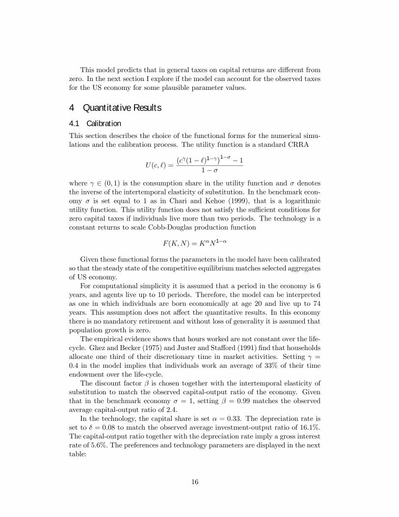
4.1 Calibration

This section describes the choice of the functional forms for the numerical simu-lations and the calibration process. The utility function is a standard CRRA

U(c, `) =

¡cγ(1− `)1−γ¢1−σ − 1

1− σwhere γ ∈ (0, 1) is the consumption share in the utility function and σ denotesthe inverse of the intertemporal elasticity of substitution. In the benchmark econ-omy σ is set equal to 1 as in Chari and Kehoe (1999), that is a logarithmicutility function. This utility function does not satisfy the sufficient conditions forzero capital taxes if individuals live more than two periods. The technology is aconstant returns to scale Cobb-Douglas production function

F (K,N) = KαN1−α

Given these functional forms the parameters in the model have been calibratedso that the steady state of the competitive equilibrium matches selected aggregatesof US economy.

For computational simplicity it is assumed that a period in the economy is 6years, and agents live up to 10 periods. Therefore, the model can be interpretedas one in which individuals are born economically at age 20 and live up to 74years. This assumption does not affect the quantitative results. In this economythere is no mandatory retirement and without loss of generality it is assumed thatpopulation growth is zero.

The empirical evidence shows that hours worked are not constant over the life-cycle. Ghez and Becker (1975) and Juster and Stafford (1991) Þnd that householdsallocate one third of their discretionary time in market activities. Setting γ =0.4 in the model implies that individuals work an average of 33% of their timeendowment over the life-cycle.

The discount factor β is chosen together with the intertemporal elasticity ofsubstitution to match the observed capital-output ratio of the economy. Giventhat in the benchmark economy σ = 1, setting β = 0.99 matches the observedaverage capital-output ratio of 2.4.

In the technology, the capital share is set α = 0.33. The depreciation rate isset to δ = 0.08 to match the observed average investment-output ratio of 16.1%.The capital-output ratio together with the depreciation rate imply a gross interestrate of 5.6%. The preferences and technology parameters are displayed in the nexttable:

16

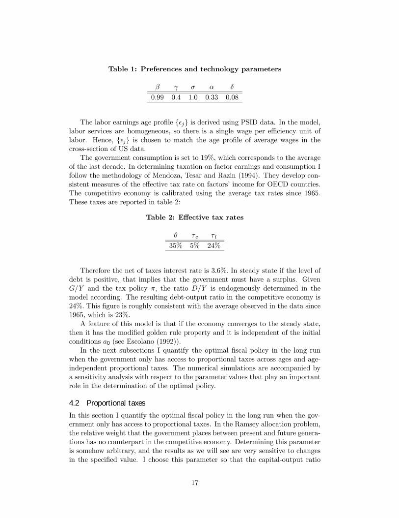
Table 1: Preferences and technology parameters

β γ σ α δ

0.99 0.4 1.0 0.33 0.08

The labor earnings age proÞle {²j} is derived using PSID data. In the model,labor services are homogeneous, so there is a single wage per efficiency unit oflabor. Hence, {²j} is chosen to match the age proÞle of average wages in thecross-section of US data.

The government consumption is set to 19%, which corresponds to the averageof the last decade. In determining taxation on factor earnings and consumption Ifollow the methodology of Mendoza, Tesar and Razin (1994). They develop con-sistent measures of the effective tax rate on factors� income for OECD countries.The competitive economy is calibrated using the average tax rates since 1965.These taxes are reported in table 2:

Table 2: Effective tax rates

θ τ c τ l

35% 5% 24%

Therefore the net of taxes interest rate is 3.6%. In steady state if the level ofdebt is positive, that implies that the government must have a surplus. GivenG/Y and the tax policy π, the ratio D/Y is endogenously determined in themodel according. The resulting debt-output ratio in the competitive economy is24%. This Þgure is roughly consistent with the average observed in the data since1965, which is 23%.

A feature of this model is that if the economy converges to the steady state,then it has the modiÞed golden rule property and it is independent of the initialconditions a0 (see Escolano (1992)).

In the next subsections I quantify the optimal Þscal policy in the long runwhen the government only has access to proportional taxes across ages and age-independent proportional taxes. The numerical simulations are accompanied bya sensitivity analysis with respect to the parameter values that play an importantrole in the determination of the optimal policy.

4.2 Proportional taxes

In this section I quantify the optimal Þscal policy in the long run when the gov-ernment only has access to proportional taxes. In the Ramsey allocation problem,the relative weight that the government places between present and future genera-tions has no counterpart in the competitive economy. Determining this parameteris somehow arbitrary, and the results as we will see are very sensitive to changesin the speciÞed value. I choose this parameter so that the capital-output ratio

17

associated with the optimal policy coincides with the competitive economy. Thatimplies setting λ = 0.947.

A summary of the results obtained for the case where the government is re-stricted to use proportional taxes across consumers in presented in table 3.

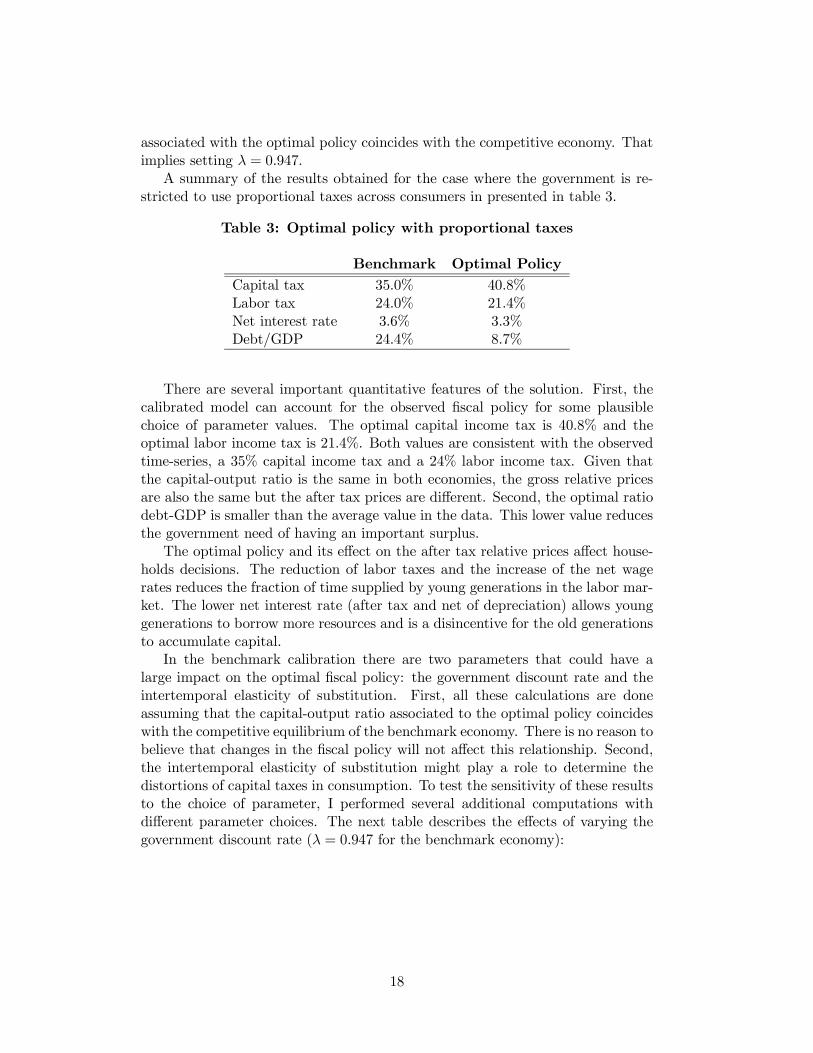
Table 3: Optimal policy with proportional taxes

Benchmark Optimal PolicyCapital tax 35.0% 40.8%Labor tax 24.0% 21.4%Net interest rate 3.6% 3.3%Debt/GDP 24.4% 8.7%

There are several important quantitative features of the solution. First, thecalibrated model can account for the observed Þscal policy for some plausiblechoice of parameter values. The optimal capital income tax is 40.8% and theoptimal labor income tax is 21.4%. Both values are consistent with the observedtime-series, a 35% capital income tax and a 24% labor income tax. Given thatthe capital-output ratio is the same in both economies, the gross relative pricesare also the same but the after tax prices are different. Second, the optimal ratiodebt-GDP is smaller than the average value in the data. This lower value reducesthe government need of having an important surplus.

The optimal policy and its effect on the after tax relative prices affect house-holds decisions. The reduction of labor taxes and the increase of the net wagerates reduces the fraction of time supplied by young generations in the labor mar-ket. The lower net interest rate (after tax and net of depreciation) allows younggenerations to borrow more resources and is a disincentive for the old generationsto accumulate capital.

In the benchmark calibration there are two parameters that could have alarge impact on the optimal Þscal policy: the government discount rate and theintertemporal elasticity of substitution. First, all these calculations are doneassuming that the capital-output ratio associated to the optimal policy coincideswith the competitive equilibrium of the benchmark economy. There is no reason tobelieve that changes in the Þscal policy will not affect this relationship. Second,the intertemporal elasticity of substitution might play a role to determine thedistortions of capital taxes in consumption. To test the sensitivity of these resultsto the choice of parameter, I performed several additional computations withdifferent parameter choices. The next table describes the effects of varying thegovernment discount rate (λ = 0.947 for the benchmark economy):

18

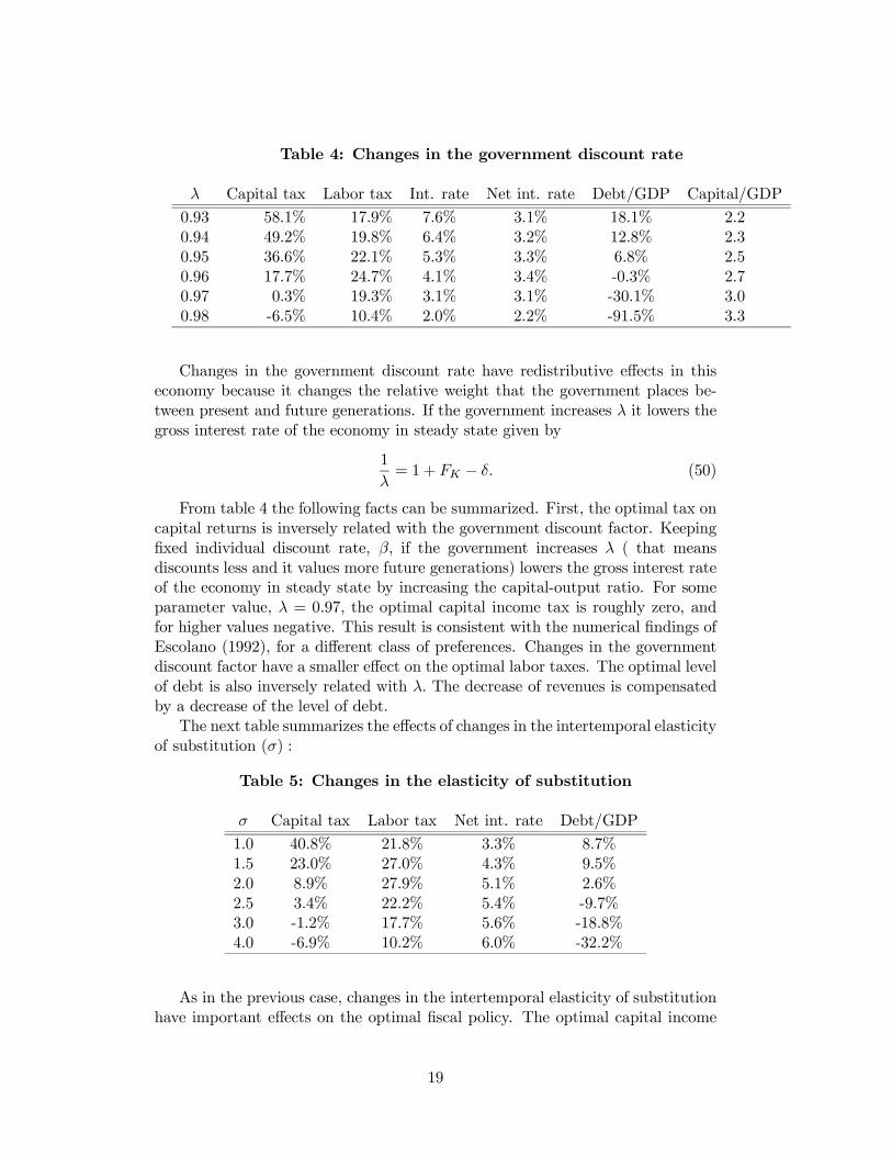
Table 4: Changes in the government discount rate

λ Capital tax Labor tax Int. rate Net int. rate Debt/GDP Capital/GDP

0.93 58.1% 17.9% 7.6% 3.1% 18.1% 2.20.94 49.2% 19.8% 6.4% 3.2% 12.8% 2.30.95 36.6% 22.1% 5.3% 3.3% 6.8% 2.50.96 17.7% 24.7% 4.1% 3.4% -0.3% 2.70.97 0.3% 19.3% 3.1% 3.1% -30.1% 3.00.98 -6.5% 10.4% 2.0% 2.2% -91.5% 3.3

Changes in the government discount rate have redistributive effects in thiseconomy because it changes the relative weight that the government places be-tween present and future generations. If the government increases λ it lowers thegross interest rate of the economy in steady state given by

1

λ= 1 + FK − δ. (50)

From table 4 the following facts can be summarized. First, the optimal tax oncapital returns is inversely related with the government discount factor. KeepingÞxed individual discount rate, β, if the government increases λ ( that meansdiscounts less and it values more future generations) lowers the gross interest rateof the economy in steady state by increasing the capital-output ratio. For someparameter value, λ = 0.97, the optimal capital income tax is roughly zero, andfor higher values negative. This result is consistent with the numerical Þndings ofEscolano (1992), for a different class of preferences. Changes in the governmentdiscount factor have a smaller effect on the optimal labor taxes. The optimal levelof debt is also inversely related with λ. The decrease of revenues is compensatedby a decrease of the level of debt.

The next table summarizes the effects of changes in the intertemporal elasticityof substitution (σ) :

Table 5: Changes in the elasticity of substitution

σ Capital tax Labor tax Net int. rate Debt/GDP

1.0 40.8% 21.8% 3.3% 8.7%1.5 23.0% 27.0% 4.3% 9.5%2.0 8.9% 27.9% 5.1% 2.6%2.5 3.4% 22.2% 5.4% -9.7%3.0 -1.2% 17.7% 5.6% -18.8%4.0 -6.9% 10.2% 6.0% -32.2%

As in the previous case, changes in the intertemporal elasticity of substitutionhave important effects on the optimal Þscal policy. The optimal capital income

19

tax is highly sensitive to assumptions about the intertemporal elasticity of sub-stitution. Auerbach and Kotlikoff (1987) use 1.5, and some other authors in envi-ronments with uncertainty have used values around 2. The optimal tax on capitalreturns is zero only for a special parametrization of the model economy, in thiscase when σ ∈ (2.5, 3.0). The optimal labor tax is not very sensitive to variationsin this parameter because the consumption and labor decisions are not affectedby σ. In general, a lower taxation is compensated with a lower debt-output ratio.

To summarize, if the government uses proportional taxes across ages, theoptimal capital tax is consistent with the observed tax for the US economy. Theoptimal Þscal policy is very sensitive to variations of the government discount rateand the intertemporal elasticity of substitution. The calibrated model can accountfor the observed capital taxes for some plausible choice of parameter values. Theconditions for zero capital taxes in steady state are much more restrictive that inthe inÞnitely-lived agent model. In the next section we study the optimal policywhen the government has access to age-dependent proportional taxes.

4.3 Age-dependent taxes

This section studies from a quantitative point of view the optimal Þscal policywith an unrestricted set of Þscal instruments. Now the government can chooseage-dependent proportional taxes. Formally that implies dropping the additionalconstraints on the marginal rates of substitution in the government problem. NextÞgure presents a summary of the numerical results for the optimal policy in thebenchmark economy:

[Insert Figure 1]

We can summarize these characteristics as follows. First, for the benchmarkcase (σ = 1), the age-speciÞc capital tax is constant across households and equalto zero. This result is consistent with Proposition 3, this type of utility functionsatisÞes the sufficient conditions for zero capital taxes if the government can useage-speciÞc taxes.8 Second, the age speciÞc labor income taxes are large anddiffer across households. For this particular parametrization labor taxes are theonly source of revenues to Þnance government expenditure. The ratio debt-GDPassociated to the optimal policy is 45.1%, almost double than the average observedin the data from 1965-1996.

As in the previous section, the quantitative analysis is accompanied by a sensi-tivity analysis with respect to the government discount rate and the intertemporalelasticity of substitution. Variations of the government discount rate, λ, do notaffect the optimal tax on capital returns as long as the utility function satisÞesthe sufficient conditions. Hence, this result is independent of the relative weightthat the government places on present and future generations. Changes in thediscount rate affect the interest rate in steady state, the higher is λ, the higher

8In this case the additional conditions that restrict the marginal rates of substitution betweenconsumption today and tomorrow are not binding. In order to satisfy the sufficient conditionsfor zero capital taxation we must allow labor taxes to differ across agents.

20

are wages in the economy. Therefore at a higher wage the Þnancial needs of thegovernment can be satisÞed with a lower labor income tax. The level of debt isadjusted to satisfy the desired capital-output ratio. For a higher values of theintertemporal elasticity of substitution the optimal capital tax across generationsis different from zero. Figure 2 displays the optimal age-speciÞc taxes for differentvalues of σ.

[Insert Figure 2]

Summarizing the effects of changes in intertemporal elasticity of substitu-tion. First, the distribution of capital taxes differs over the life cycle. For theparametrized version of the model, if the government can use a complete set ofinstruments, then the age proÞle capital tax pattern implies subsidizing asset re-turns of the young generations in the economy and taxing at high rates the assetreturns of old generations. Changes in the elasticity of substitution do not affectthe average capital income tax over the life cycle, which is zero. Second, noticethat an increase in σ does not substantially affect the distribution of capital taxesacross generations, but it lowers the labor-speciÞc taxes for all ages.. Finally, bothlabor income taxes and the ratio debt-output are decreasing in σ. For σ = 1.5,the debt-output ratio is 23.1% and for σ = 2 only 3.9%. For higher values of σ,this ratio is negative.

5 Conclusions

This paper provides, from a theoretical and quantitative point of view, an expla-nation of why the observed taxes on capital returns are larger than what standardtheory predicts, not taxing capital at all. Using a stylized economy with inter-generational redistribution, I derive a sufficient condition to check whether theoptimal policy implies zero capital taxes, and I show that commonly used utilityfunctions in the macro and public Þnance literature violate this condition. There-fore, when heterogeneity is due to an intergenerational factor, we should expecttaxes on capital returns to be different from zero. For a version of the model,calibrated to the US economy, the main results are: Þrst, if the government isrestricted to use proportional taxes across generations, the model can account forthe observed capital and labor income taxes. Second, if the government can usespeciÞc taxes for each generation, then the age proÞle capital tax pattern impliessubsidizing asset returns of the younger generations and taxing at higher ratesthe asset returns of the older ones.

21

6 References

Aiyagari, R. (1995), �Optimal Capital Income Taxation with Incomplete Markets,Borrowing Constraints, and Constant Discounting�, Journal of Political Economy,103: 158-75.

Atkinson, A. B. and A. Sandmo (1980), �Welfare Implications of the Taxationof Savings�, Economic Journal, 90: 519-549.

Atkinson, A. B. and J. Stiglitz (1980), Lectures on Public Economics. McGraw-Hill, New York.

Auerback, A.J. and L.J. Kotlikoff (1987), Dynamic Fiscal Policy. CambridgeUniversity Press. Cambridge.

Calvo, G. (1978), �On the Time Consistency of Optimal and Monetary Policyin a Monetary Economy�, Econometrica 46: 1411-1428.

Chamley, C. (1986), �Optimal Taxation of Capital Income in General Equi-librium with InÞnite Lives�, Econometrica 54: 607-622.

Chari, V.V. and P.J. Kehoe (1990), �Sustainable Plans�, Journal of PoliticalEconomy, 98: 783-802.

Chari, V.V., L.J. Christiano and P.J. Kehoe (1994), �Optimal Fiscal Policyin a Business Cycle Model�, Journal of Political Economy, 102: 617-652.

Chari, V.V., and P.J. Kehoe (1999), �Optimal Fiscal and Monetary Policy�,in Handbook of Macroeconomics, vol , Edited by J.B. Taylor and M. Woodford.Elsevier.

Diamond, P.A. (1965), �National Debt on a Neoclassical Growth Model�,American Economic Review, 55: 1126-1150.

Domeij, D. and J. Heathcote (2000), �Capital versus Labor Income Taxationwith Heterogeneous Agents�, Mimeo, Stockholm School of Economics.

Erosa, A. and M. Gervais (2000), �Optimal Fiscal Policy in Life-Cycle Economies�,Federal Reserve Bank of Richmond Working Paper 00-2.

Escolano, J. (1992), �Optimal Taxation in Overlapping Generations Models�,Mimeo. University of Minnesota.

Ghez, G. and G.S. Becker (1975), The allocation of time and Goods over theLife Cycle, New York: Columbia University Press.

Golosov, M. N. Kocherlakota and A. Tsyvinski (2001), �Optimal Indirect andCapital Taxation�, Working Paper 615, Federal Reserve Bank of Minneapolis.

Jones, L.E., R.E. Manuelli and P.E. Rossi (1997), �On the Optimal Taxationof Capital Income�, Journal of Economic Theory, 73: 93�117.

Judd, K.L. (1985), �Redistributive Taxation in a Simple Perfect ForesightModel�, Journal of Public Economics, 28: 59-83.

Judd, K.L. (1999), �Optimal Taxation and Spending in General CompetitiveGrowth Models�, Journal of Public Economics, 71: 1-263.

Juster, F.T. and F.P. Stafford (1991), �The Allocation of Time: EmpiricalFindings, Behaviour Models, and Problem Measurement�, Journal of EconomicLiterature 29: 471-522.

Klein, P. and J.V. Ríos-Rull (1999), �Time Consistent Fiscal Policy�, MimeoUniversity of Pennsylvania.

22

Kydland, F.E. and Prescott, E.C. (1977), �Rules Rather than Discretion: TheInconsistency of Optimal Plans�, Journal of Political Economy, 85: 473-91.

Lucas, R.E. Jr. (1990), �Supply-Side Economics: An Analytical Review�,Oxford Economics Papers, 42: 293-316.

Lucas, R.E. Jr. and N.L. Stokey (1983), �Optimal Fiscal and Monetary Policyin an Economy without Capital�, Journal of Monetary Economics, 12: 55-93.

Mendoza, E.G., A. Razin and L.L. Tesar (1994), �Effective Tax Rates inMacroeconomics: Cross-Country Estimates of Tax Rates on Factor Incomes andConsumption,� Journal of Monetary Economics; 34: 297-323.

Pestieau, P.M. (1974), �Optimal Taxation and Discount Rate for Public In-vestment in a Growth Setting,� Journal of Public Economics; 3: 217�235.

Phelan, C. and E. Stacchetti (1999), �Sequential Equilibrium in a RamseyTax Model�, Research Department Staff Report 258, Federal Reserve Bank ofMinneapolis.

Razin, A. and E. Sandka (1995), �The Status of Capital Income Taxation inthe Open Economy�, FinanzArchiv, 52: 21-32.

Samuelson, P.A. (1958), �An Exact Consumption-Loan Model of Interest withor without the Social Contrivance of Money�, Journal of Political Economy, 66:467-482.

Stokey, N.L. (1991), �Credible Public Policies�, Journal of Economic Dynam-ics and Control, 15: 627-656.

23

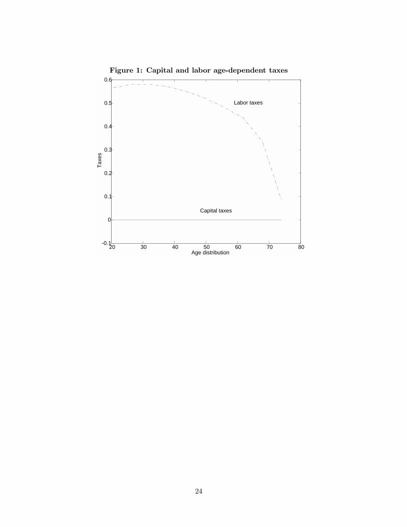
Figure 1: Capital and labor age-dependent taxes

20 30 40 50 60 70 80-0.1

0

0.1

0.2

0.3

0.4

0.5

0.6

Age distribution

Taxe

sLabor taxes

Capital taxes

24

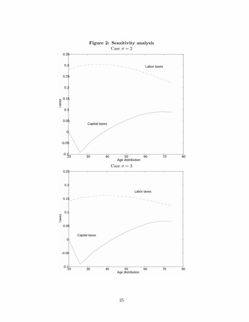
Figure 2: Sensitivity analysisCase σ = 2

20 30 40 50 60 70 80-0.1

-0.05

0

0.05

0.1

0.15

0.2

0.25

0.3

0.35

Age distribution

Taxe

s

Labor taxes

Capital taxes

Case σ = 3

20 30 40 50 60 70 80-0.1

-0.05

0

0.05

0.1

0.15

0.2

0.25

Age distribution

Taxe

s

Labor taxes

Capital taxes

25