Optimal Diversification:Reconciling Theory and Evidence

Joao Gomes and Dmitry Livdan∗

January, 2003

Abstract

In this paper we show that the main empirical findings about firm diversificationand performance are consistent with the maximization of shareholder value. In ourmodel, diversification allows a firm to explore better productive opportunities whiletaking advantage of synergies. By explicitly linking the diversification strategies of thefirm to differences in size and productivity, our model provides a natural laboratoryto investigate quantitatively several aspects of the relationship between diversificationand performance. Specifically, we show that our model is able to rationalize both theevidence on the diversification discount (Lang and Stulz (1994)) and the documentedrelation between diversification and firm productivity (Schoar (2002)).

JEL classification: D21, G32, G34Keywords: Diversification; Corporate Strategy; Diversification Discount; Total

Factor Productivity and Size;

∗The Wharton School, University of Pennsylvania. E-mail: gomesj@wharton.upenn.edu, anddlivdan@wharton.upenn.edu. We are grateful to Andrew Abel, Michael Brandt, Domenico Cuoco, JanEberly, Simon Gervais, Armando Gomes, Francisco Gomes, Gary Gorton, John Graham, Skander Van denHeuvel, Rich Kihlstrom, Leonid Kogan, Jan Mahrt-Smith, Vojislav Maksimovic, Andrew Metrick, GordonPhillips, Tom Sargent, Jeremy Stein, and an anonymous referee, as well as seminar participants at Kellogg,Wharton, Penn State, the 2002 SED and Econometric Society Meetings, and the 2003 AFA meetings.Financial Support from the Rodney L. White Center for Financial Research is gratefully acknowledged. Thispaper combines our earlier papers ”Optimal Diversification” and ”The Performance of Optimally DiversifiedFirms: Reconciling Theory and Evidence”.

Empirical work on firm diversification has often been interpreted as supporting the view

that conglomerates are inefficient. Findings such as the fact that conglomerates trade at

a discount, relative to a portfolio of comparable stand-alone firms, have led researchers to

believe that diversification destroys value.1 Popular explanations for this “diversification

discount” have generally emphasized the agency and behavioral problems associated with

the existence of conglomerates.2 Unfortunately, this view of diversification creates at least

two difficulties for researchers. First, while addressing the effects of diversification on

performance, agency models often fail to answer the more fundamental economic question

of why diversified firms exist at all, as diversification is often ex-ante inefficient. Second, the

empirical predictions of these agency-based models are usually very hard to quantify and

thus quite difficult to test. As a consequence, direct evidence supporting this agency view

is quite limited. Instead, support typically comes from the perceived failures of competing

theories.

In this paper we show that the main empirical regularities about firm diversification are

broadly consistent with a neoclassical view of efficient firm diversification. In our model, firms

diversify for two reasons. First, diversification allows firms to take advantage of economies

of scope by eliminating redundancies across different activities and lowering fixed costs of

production. Second, diversification allows a mature, slow growing, firm to explore attractive

new productive opportunities. We formalize this concept by assuming that production

activities exhibit decreasing returns to scale. As scale grows, returns decrease, eventually

leading the firm to search for profit opportunities in new activities.

In contrast to standard agency arguments, the structure of our model provides a natural

environment to investigate quantitatively the role of firm diversification on performance.

1

Since the model generates an artificial cross-sectional distribution of firms, we are able to

directly compare our results with the available empirical evidence.

We have two main sets of findings. First, the model predicts that diversified firms have,

on average, a lower value of Tobin’s Q than focused firms, as documented by Lang and

Stulz (1994). This happens despite the fact that diversification is optimal and there is no

source of inefficiency in our model. The intuition, however, is simple. In our model, firms

diversify only when they become relatively unproductive in their current activities. It is this

endogenous selection mechanism that accounts for the lower valuation of diversified firms.

Second, because our model explicitly links productivity with corporate diversification, we can

also address recent evidence on the effects of diversification on productivity (Schoar (2002)).

We find that, just as in the data, our model predicts that firms following diversification

strategies also experience empirically plausible productivity losses.

This emphasis on the importance of firm selection in accounting for the performance of

conglomerates effectively presents a theoretical foundation for the recent empirical findings

by Chevalier (2001), Villalonga (2001), and Campa and Kedia (2002). Although their exact

sources and methodologies differ, all of these papers are part of a growing empirical literature

suggesting that sample selection accounts for most, if not all, of the ex-post differences

between conglomerates and specialized firms.3

More broadly, our work is also part of a recent strand of literature that emphasizes a

view of conglomerates as profit maximizing firms. Nevertheless, all of them still assume that

diversification reduces firm value: while conglomerates allocate resources efficiently (profit

maximization), they are still endowed with lower profit opportunities than a specialized firm

(diversification is value reducing).

2

For example, Matsusaka (2001) models diversification as an intermediate, and less

productive, stage in a search process over industries that best match the firm’s organizational

capabilities. When the perfect match is found, a firm eventually specializes. Bernardo and

Chowdhry (2002) explain the diversification discount by assuming that specialized firms have

growth options allowing them to diversify in the future. Conglomerates on the other hand,

are firms who have exercised these options and are thus less valuable to investors.

Closest to our model is the work of Maksimovic and Phillips (2002) who first formalize

the idea that diversification decisions can be understood as the optimal response of firms

to industry or sectoral shocks. Using a static linear quadratic model, they show that firms

will become conglomerates only when they face similar profit opportunities across sectors.

Specialized firms, on the other hand, are usually much more productive in their chosen

activities. Their paper also provides strong supporting evidence for this view. In their

model conglomerates are valued at a premium relative to small specialized firms and at a

discount relative to large specialized firms. However, they also assume that firms must incur

extra costs when they produce in more than one industry.

Thus, while our dynamic environment does incorporate features from these models, our

analysis differs in one crucial way. In our model conglomerates are not assumed to be

ex-ante less efficient. Thus our model generates a diversification discount endogenously, an

explanation that seems consistent with recent empirical evidence, and questions the common

interpretation of the diversification discount as evidence of inefficiency. This endogenous

relation between productivity and diversification is also present in Maksimovic and Phillips

(2002) and Inderst and Muller (2003). Our dynamic setting however allows us to also account

for the interaction between productivity and firm size as joint determinants of the decision to

3

diversify. As we will see this allows us to better account for the existing empirical evidence.

In addition to this key distinction, our model also provides a unified and consistent

explanation for much of the empirical evidence by endogenously linking productivity, size,

and valuations to diversification strategies. Finally, our approach relies on the detailed

quantitative evaluation of an artificial panel of firms generated by solving a fully specified

general equilibrium environment. Thus our framework is able to produce a well-defined

cross-sectional distribution of firms that provides both a reasonable description of the data

and a natural ground to examine the quantitative implications of our model.

Finally, our work also offers a useful framework to study the natural boundaries of the

firm in the context of a neoclassical environment. While our model is silent about the exact

micro-foundations for the interactions between (and within) firms (for example, internal

capital markets, incomplete contracts, and power relationships within firms), it provides

something of a reduced form approach that is well suited for detailed empirical study, a

serious difficulty in this field of research.

The rest of this paper is organized as follows. Section I details the basic economic

environment and discusses our main assumptions. Section II provides a quantitative

evaluation of our model and establishes its main empirical implications. Section III

concludes.

I Model

A pattern that emerges from much of the relevant empirical evidence is one of substantial

firm heterogeneity across a number of different characteristics such as firm size, firm growth,

as well as investment and diversification strategies. It is therefore crucial that our framework

4

is consistent with this evidence and thus able to produce a well-defined cross-sectional

distribution of firms that provides a reasonable description of the data.

Our theoretical approach is then based on a industry equilibrium environment with

heterogeneous firms, along the lines of Hopenhayn (1992) and Gomes (2001). Our economy

consists of 2 sectors: households and firms. The core of the analysis is our description

of the production sector, where a large number of firms is engaged in the production of

the consumption good. The role of households is limited and summarized by a single

representative household making optimal consumption and portfolio decisions.

A Firms

The production side of the economy consists of a large number of firms and two separate

industries or sectors. While the model can be augmented to include more sectors, this would

make the analysis unnecessarily complicated. Empirically, the effects of diversification on

performance are most notable when firms first expand from one to two segments, with

additional expansions having only marginal effects on performance (Lang and Stulz (1994)).

A.1 Description

We assume that time is discrete and the horizon is infinite. In each time period t, a firm

can either be focused in sector st = 1, 2 or operate in both sectors simultaneously, in which

case we will say that a firm is diversified and set st = 1 + 2 = 3. We assume that sectoral

mobility is costly so that specialized firms cannot simply move all resources from sector 1 to

sector 2 (say). Formally, we assume that:

st ∈{ {st−1, 3}, st−1 = 1, 2

{1, 2, 3}, st−1 = 3(1)

5

In other words, a firm that has previously been focused in sector s can only choose to

remain in sector s (st = st−1), or to expand to both sectors (st = 3). Diversified firms,

however, face no restrictions: they can either remain diversified, or they can refocus on a

single industry. This costly mobility ensures that a firm must diversify before focusing on

entirely new activities, a pattern that is consistent with the data.4

The outcome of production in sector s, during period t, is the final good yst . For simplicity,

we assume that the goods are perfect substitutes so that the relative price between y1t and y2

t

is always equal to 1. Production in either sector requires two inputs: capital or productive

capacity, kt, and labor, lt, and is subject to a technology shock zst . Labor is hired at the

competitive wage rate Wt > 0, but capacity is owned by the firm. Production possibilities

for an individual firm operating in sector s are described by a Cobb-Douglas production

function:

yst = ezs

t kαkt lαl

t , 0 < αk + αl < 1, (2)

where αk and αl are the output elasticities of capital and labor, respectively. The restrictions

on these coefficients guarantee that production in each sector exhibits decreasing returns to

scale, so that returns fall as the firm grows.

Productivity levels are firm specific and cannot be traded. We assume that productivity

in each sector s follows a simple AR(1) process

zst = ρzs

t−1 + εst , (3)

where each εst is a normal random variable with mean zero and variance σ2. For simplicity

we also assume that there is no cross-correlation between the shocks in the two sectors. To

save on notation we also define the productivity vector zt = (z1t , z

2t ).

6

Finally, total firm capacity is described by the law-of-motion

kt+1 = (1 − δ)kt + it, (4)

where it denotes gross investment spending, and δ is the depreciation rate of capital. Thus,

new investment, it, becomes productive only at the beginning of the next period.

The timing of the decisions is illustrated in Figure 1.

Every firm arrives at period t with a pre-chosen level of capacity kt. Before any activity

takes place the firm observes the (firm-specific) vector of productivity levels in both sectors,

zt. With this information at hand, each firm makes the following choices during the period

t:

• the optimal sectoral decision for the current period, st, by choosing whether to operate

one (st = 1 or 2) or both (st = 3) production units in period t;

• the optimal allocation of capital and labor across its activities;

• how much to invest for the future, it, and, as a consequence, the total amount of

capacity to install at the beginning of the next period, kt+1.

A firm that chooses to focus its activities in sector st alone generates the following profits

during period t:

π(st, kt, zt; Wt) = maxlt

{ezs

t kαkt lαl

t − Wtlt − f}

, st = 1, 2 (5)

where f ≥ 0 is a fixed cost of production that must be paid if the firm is active in sector s.5

7

Conversely, if the firm chooses to be diversified (so that st = 3), profits are described by:

π(3, kt, zt; Wt) = maxlt,θt

{ez1

t (θtkt)αk(θtlt)

αl + ez2t ((1 − θt)kt)

αk((1 − θt)lt)αl (6)

−Wtlt − (2 − λ)f} ,

s.t. 0 ≤ θt ≤ 1,

where θt denotes the fraction of resources (capital and labor) that the diversified firm

allocates to sector 1 in period t.6 Because diversified firms operate in both sectors, they

face larger fixed costs of production. However, equation (6) embeds our assumption that

they can eliminate redundancies and thus save a fraction λ/2 of the combined costs in each

sector. Thus, a conglomerate pays only fixed costs in the amount (2 − λ)f .

The solution to these static optimization problems yields optimal decision rules for total

firm employment, lt = l(st, kt, zt; Wt), the size of each segment, θt = θ(st, kt, zt; Wt), as well

as total production, yt = y(st, kt, zt; Wt).

A.2 Discussion

Our environment is constructed to incorporate the main incentives for the creation of

conglomerates identified by the literature on firm diversification. Somewhat loosely our

model emphasizes some of the most popular advantages of firm diversification: “synergies”

and the exploration of “free” cash flows.

Synergies are created through the elimination of redundancies across business lines, such

as overhead. In our model, this feature is captured by the savings parameter λ. Such dilution

of costs generates a form of economies of scope and creates a benefit to firm diversification

that cannot be replicated by shareholders. It is this key advantage that separates our work

from the existing literature. In our model, conglomerates not only operate efficiently, but

8

they also create value to investors. As a result the resulting diversification discount in our

model is entirely driven entirely by the endogenous nature of the diversification decision.

In addition to this key feature, our model also assumes the existence of decreasing returns

to scale in each sector. This assumption generates something like a “free cash flow” effect:

as the firm grows in size, marginal productivities fall and it becomes unprofitable for the

firm to invest additional resources in on-going activities. Instead, the firm can better use

resources by exploring new production possibilities. Thus, diversification is more likely to

be optimal for large firms, since it enables them to overcome the decreasing returns nature

of the single sector technology. This feature is also consistent with the empirical observation

that large firms are much more likely to become diversified.

Decreasing returns to scale are also used by Santalo (2001) and Maksimovic and Phillips

(2002). Santalo (2001) constructs a model where the diversification discount is attributed by

the ”size discount” induced by decreasing returns. However, much of the empirical evidence

suggests that decreasing returns alone are not sufficient since the diversification discount

seems to survive after one controls for the size of the firm. Maksimovic and Phillips (2002)

use a linear quadratic example to show how decreasing returns to scale can provide a natural

bound to the size of the firm and thus create an incentive to diversification. Because they do

not have fixed costs in their model however, firms would never find it optimal to be focused.

To overcome this, they instead must assume that conglomerates have higher production costs

than those of two focused firms combined.

In addition to these core advantages, conglomerates also benefit from two additional

features of our environment. They have more options than stand-alone firms (the mobility

restriction (1)). Although this is not a crucial feature of our model, it stands in contrast

9

to Bernardo and Chowdry (2002), who rationalize the diversification discount by assuming

that focused firms have more options than conglomerates.

Finally, since the productivity shocks z1t and z2

t are not perfectly correlated (as in equation

(3) above), diversification allows a firm to both explore alternative profit opportunities and

lower exposure to cash flow risk. This idea of conglomerates as the optimal response of firms

to sectoral variations in profit opportunities was also first introduced to this literature by

Maksimovic and Phillips (2002). However, in the absence of trading frictions, this feature is

not valued by investors in general equilibrium since it can be easily replicated by a portfolio

of stand-alone firms.

Thus, in our model production is more efficient and resources are saved, when operations

are combined in a conglomerate. Hence, unlike much of the literature, our model captures

some of the most plausible benefits to corporate diversification while abstracting from any

of its potential drawbacks, such as those induced by agency or behavioral problems.

Emphasizing these advantages of the conglomerates ensures that a model does not

deliver a diversification discount “by assumption”. Since conglomerates have generally

more resources and better opportunities in our model, their low valuation can only be the

endogenous outcome of self-selection and not the obvious consequence of assuming that

focused firms are, a priori, better. As a number of recent studies suggest, this explanation

seems to consistent with the available evidence.

A.3 Optimality

Let (s, k, z) denote the state for a firm that was active in sector s in period t−1, has k units

of installed capacity at the beginning of period t, and faces a vector of productivity shocks

10

z. The optimal behavior of this firm can be summarized by the value function v(s, k, z; W ),

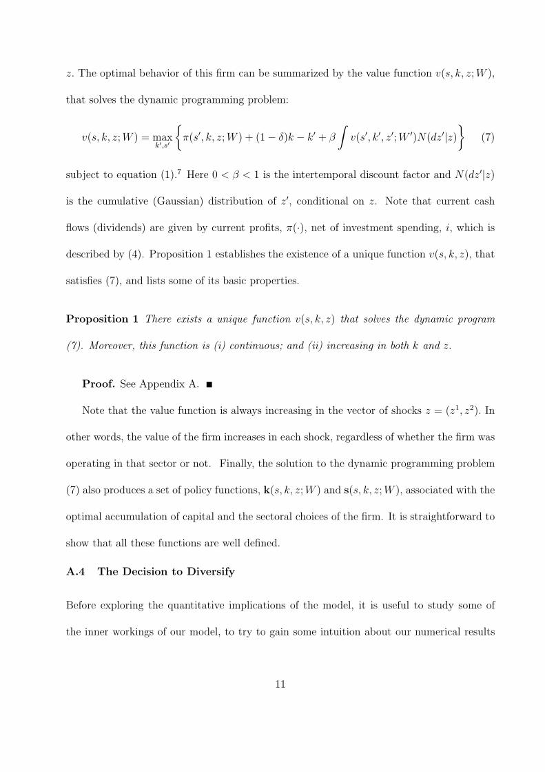
that solves the dynamic programming problem:

v(s, k, z; W ) = maxk′,s′

{π(s′, k, z; W ) + (1 − δ)k − k′ + β

∫v(s′, k′, z′; W ′)N(dz′|z)

}(7)

subject to equation (1).7 Here 0 < β < 1 is the intertemporal discount factor and N(dz′|z)

is the cumulative (Gaussian) distribution of z′, conditional on z. Note that current cash

flows (dividends) are given by current profits, π(·), net of investment spending, i, which is

described by (4). Proposition 1 establishes the existence of a unique function v(s, k, z), that

satisfies (7), and lists some of its basic properties.

Proposition 1 There exists a unique function v(s, k, z) that solves the dynamic program

(7). Moreover, this function is (i) continuous; and (ii) increasing in both k and z.

Proof. See Appendix A.

Note that the value function is always increasing in the vector of shocks z = (z1, z2). In

other words, the value of the firm increases in each shock, regardless of whether the firm was

operating in that sector or not. Finally, the solution to the dynamic programming problem

(7) also produces a set of policy functions, k(s, k, z; W ) and s(s, k, z; W ), associated with the

optimal accumulation of capital and the sectoral choices of the firm. It is straightforward to

show that all these functions are well defined.

A.4 The Decision to Diversify

Before exploring the quantitative implications of the model, it is useful to study some of

the inner workings of our model, to try to gain some intuition about our numerical results

11

below. Accordingly, this section attempts to shed some light on the optimal diversification

decision of an individual firm.

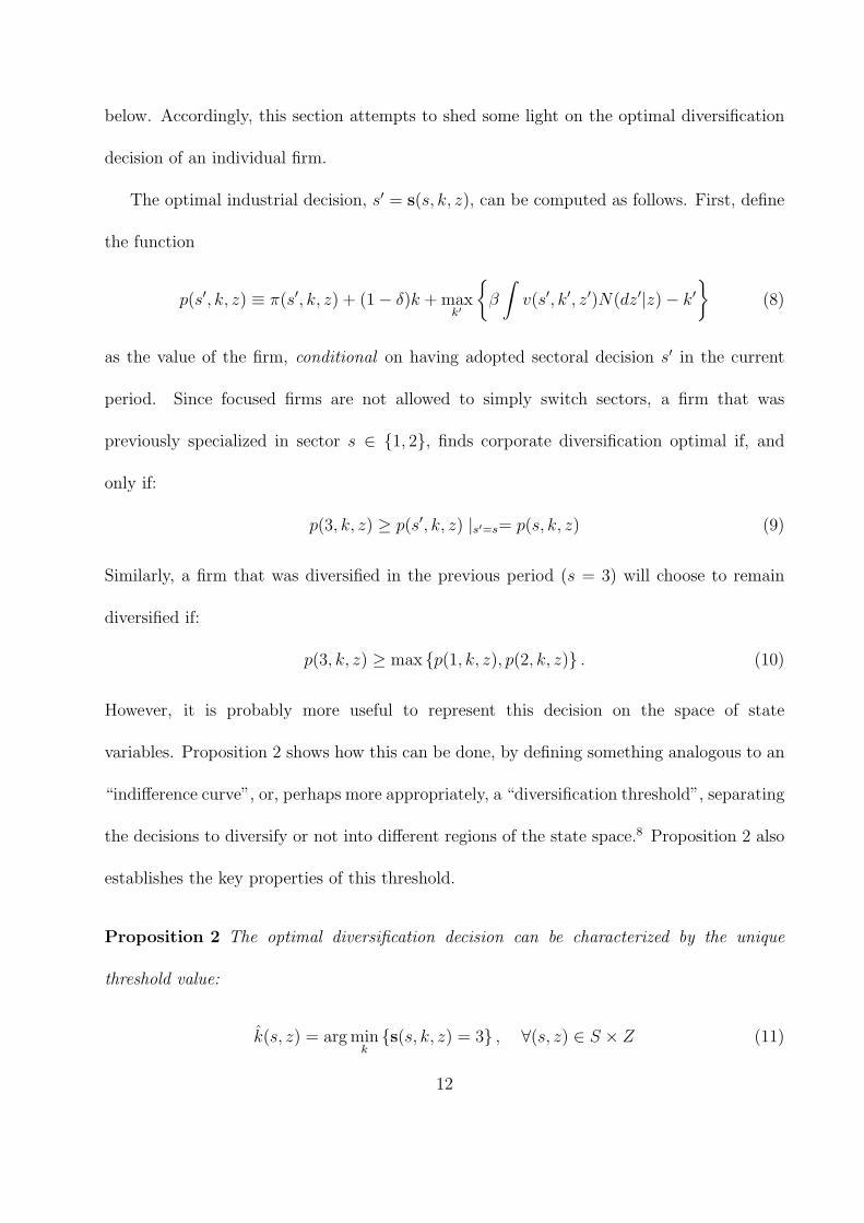
The optimal industrial decision, s′ = s(s, k, z), can be computed as follows. First, define

the function

p(s′, k, z) ≡ π(s′, k, z) + (1 − δ)k + maxk′

{β

∫v(s′, k′, z′)N(dz′|z) − k′

}(8)

as the value of the firm, conditional on having adopted sectoral decision s′ in the current

period. Since focused firms are not allowed to simply switch sectors, a firm that was

previously specialized in sector s ∈ {1, 2}, finds corporate diversification optimal if, and

only if:

p(3, k, z) ≥ p(s′, k, z) |s′=s= p(s, k, z) (9)

Similarly, a firm that was diversified in the previous period (s = 3) will choose to remain

diversified if:

p(3, k, z) ≥ max {p(1, k, z), p(2, k, z)} . (10)

However, it is probably more useful to represent this decision on the space of state

variables. Proposition 2 shows how this can be done, by defining something analogous to an

“indifference curve”, or, perhaps more appropriately, a “diversification threshold”, separating

the decisions to diversify or not into different regions of the state space.8 Proposition 2 also

establishes the key properties of this threshold.

Proposition 2 The optimal diversification decision can be characterized by the unique

threshold value:

k(s, z) = arg mink

{s(s, k, z) = 3} , ∀(s, z) ∈ S × Z (11)

12

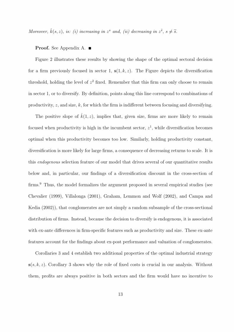
Moreover, k(s, z), is: (i) increasing in zs and, (ii) decreasing in zs, s �= s.

Proof. See Appendix A.

Figure 2 illustrates these results by showing the shape of the optimal sectoral decision

for a firm previously focused in sector 1, s(1, k, z). The Figure depicts the diversification

threshold, holding the level of z2 fixed. Remember that this firm can only choose to remain

in sector 1, or to diversify. By definition, points along this line correspond to combinations of

productivity, z, and size, k, for which the firm is indifferent between focusing and diversifying.

The positive slope of k(1, z), implies that, given size, firms are more likely to remain

focused when productivity is high in the incumbent sector, z1, while diversification becomes

optimal when this productivity becomes too low. Similarly, holding productivity constant,

diversification is more likely for large firms, a consequence of decreasing returns to scale. It is

this endogenous selection feature of our model that drives several of our quantitative results

below and, in particular, our findings of a diversification discount in the cross-section of

firms.9 Thus, the model formalizes the argument proposed in several empirical studies (see

Chevalier (1999), Villalonga (2001), Graham, Lemmon and Wolf (2002), and Campa and

Kedia (2002)), that conglomerates are not simply a random subsample of the cross-sectional

distribution of firms. Instead, because the decision to diversify is endogenous, it is associated

with ex-ante differences in firm-specific features such as productivity and size. These ex-ante

features account for the findings about ex-post performance and valuation of conglomerates.

Corollaries 3 and 4 establish two additional properties of the optimal industrial strategy

s(s, k, z). Corollary 3 shows why the role of fixed costs is crucial in our analysis. Without

them, profits are always positive in both sectors and the firm would have no incentive to

13

focus, given the assumption of decreasing returns to scale. Corollary 4 shows that if synergies

are sufficiently large there is never an incentive for the firm to be focused.

Corollary 3 In the absence of fixed costs (f = 0), diversification is always optimal.

Proof. See Appendix A.

Corollary 4 Suppose f > 0. Diversification is the optimal corporate strategy if λ ≥ 1, i.e.

synergies are sufficiently large.

Proof. See Appendix A.

B Aggregation and Equilibrium

To provide a detailed evaluation of the implications of our model, we need to construct an

artificial panel of firms that can then be used to examine the available empirical evidence.

We can do this by aggregating the individual decisions of every firm in the economy and

computing the equilibrium in our model. Since each firm can be described by the (s, k, z),

the cross-sectional distribution of firms is completely summarized by a measure, µ(s, k, z),

defined over this state space. The law of motion for µ is given by:

µ′(s′, k′, z′) =

∫1{k′=k(s,k,z;W )} × 1{s′=s(s,k,z;W )}N(z′|dz)µ(ds, dk, z), (12)

where 1{.} is an indicator function that equals 1 if the argument is satisfied and 0

otherwise. Intuitively, next period’s cross-sectional distribution of firms is determined by

combining the exogenous transition probabilities implied by N(·) with the endogenous ones,

prescribed by the optimal policies for capacity, k(s, k, z), and sectoral choices, s(s, k, z). For

14

empirical purposes we are interested in the properties of a stationary equilibrium where this

distribution does not depend on initial conditions, so that µ′ = µ.

To close the model, we must offer a description of market demand for the final goods

produced, as well as the supply of labor input. While it is easy to provide reduced form

expression for these functions, it is also straightforward to show how this can be done in

general equilibrium by adding a very stylized description of household/shareholder behavior.

Specifically, we summarize the household sector with a single representative agent deriving

utility from leisure, L, and consumption, C, and income from wages, W , and dividends,

D. Without aggregate uncertainty, all aggregate quantities and prices are constant and the

consumer problem collapses to the static representation:

maxC,L

U = ln(C − AL) (13)

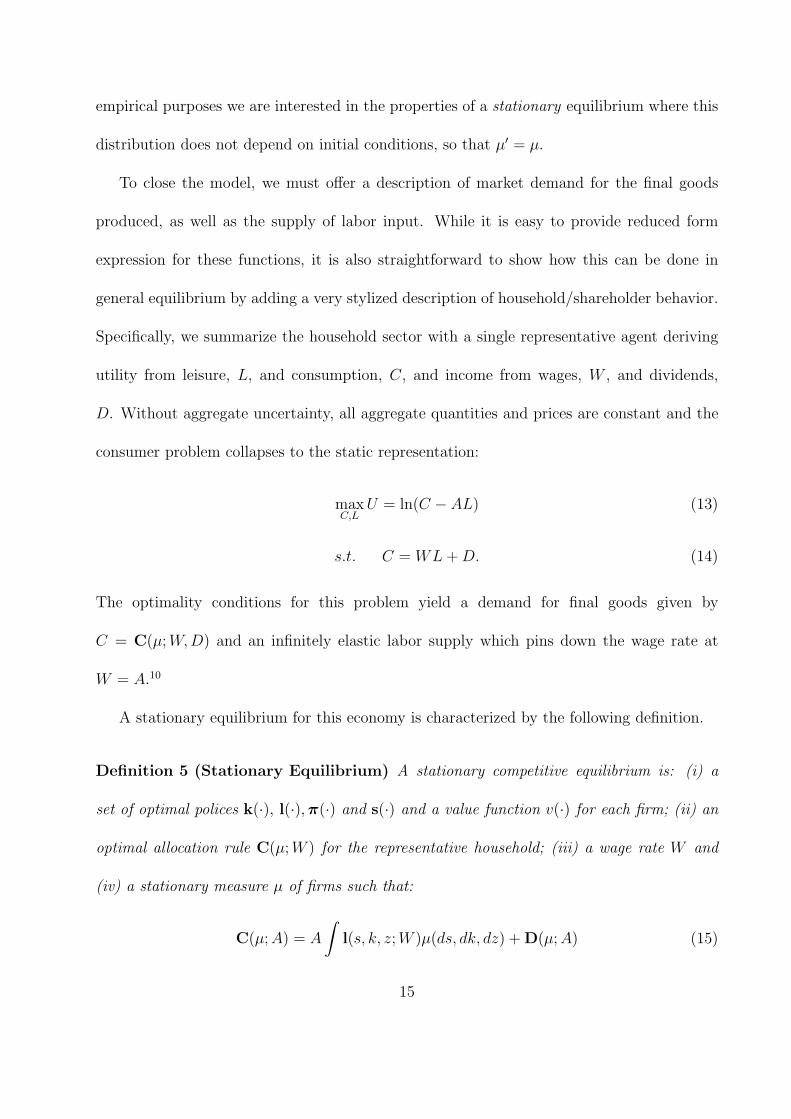
s.t. C = WL + D. (14)

The optimality conditions for this problem yield a demand for final goods given by

C = C(µ; W,D) and an infinitely elastic labor supply which pins down the wage rate at

W = A.10

A stationary equilibrium for this economy is characterized by the following definition.

Definition 5 (Stationary Equilibrium) A stationary competitive equilibrium is: (i) a

set of optimal polices k(·), l(·),π(·) and s(·) and a value function v(·) for each firm; (ii) an

optimal allocation rule C(µ; W ) for the representative household; (iii) a wage rate W and

(iv) a stationary measure µ of firms such that:

C(µ; A) = A

∫l(s, k, z; W )µ(ds, dk, dz) + D(µ; A) (15)

15

Equation (15) also summarizes labor market equilibrium, by imposing W = A. It also

uses the fact that aggregate dividends are given by11

D(µ; A) =

∫π(s, k, z; A)µ(ds, dk, dz) −

∫(k(s, k, z; A) − (1 − δ)k) µ(ds, dk, dz). (16)

Given our assumptions, establishing the existence of a stationary competitive equilibrium

is immediate.12 Although the definition seems abstract and its computation is non-trivial,

this equilibrium concept is the key to our analysis. It delivers a non-degenerate cross-sectional

distribution of firms, µ, which provides us with an artificial dataset of firms of different size,

productivities, and more importantly, diversification strategies. With this information at

hand we are ready to address the key empirical findings in this area.

II Quantitative Results

Computing the stationary equilibrium involves two steps. First, we must specify parameter

values. These must be selected to be consistent with either long run properties of the

data (unconditional first moments) or with prior empirical evidence. Second, we develop

and implement a numerical algorithm capable of approximating the stationary equilibrium

up to an arbitrarily small error. Appendix B describes this procedure in detail. With

the equilibrium computed, we focus on two key empirical issues. Section B investigates the

model’s implications for the so-called “diversification discount”, by comparing our predictions

with the results in Lang and Stulz (1994). Since our model implies that diversification is

driven by productivity differentials, it is important to investigate its predictions for the

relation between firm diversification and productivity. Section C explores this issue by

comparing our results with the empirical evidence in Schoar (2002).

16

A Calibration and Summary Statistics

Since most data is available at an annual frequency, we assume that a time period in the

model corresponds to one year. The calibration exercise is divided in two parts. First, we

use independent evidence on the degree of returns to scale (Burnside’s (1996)) to set the

output elasticities αl = 0.65 and αk = 0.3. The rate of depreciation in the capital stock is

set to 0.1, a value close to that found in the data by Gomes (2001).

The four remaining parameters, f, λ, σ, and ρ, cannot be individually identified from

the available data. Instead, they are chosen so that the model is able to approximate the

unconditional moments on the panel studied by Lang and Stulz (1994) for Compustat. Since

the main stylized facts are, in effect, conditional moments, or regressions, from this panel, this

seems appropriate. Accordingly, we select these parameters so that the model approximates

the cross-sectional mean and dispersion of Tobin’s Q, the fraction of diversified firms in the

sample, and the average level of Q for conglomerates.13

Table I summarizes our calibration procedure while Table II compares the key summary

statistics generated by the stationary equilibrium of the model with those of the Compustat

dataset used by Lang and Stulz (1994). Although our model calibration does not reproduce

these four statistics exactly, the artificial sample is reasonably similar to its empirical

counterpart, particularly in terms of cross-sectional dispersion and the relative weight of

conglomerates in the sample, the two crucial elements for statistical inference.

B Diversification Discount

Most empirical studies on the efficiency of conglomerates examine the relation between

diversification and the value of the firm, usually measured by Tobin’s (average) Q.14

17

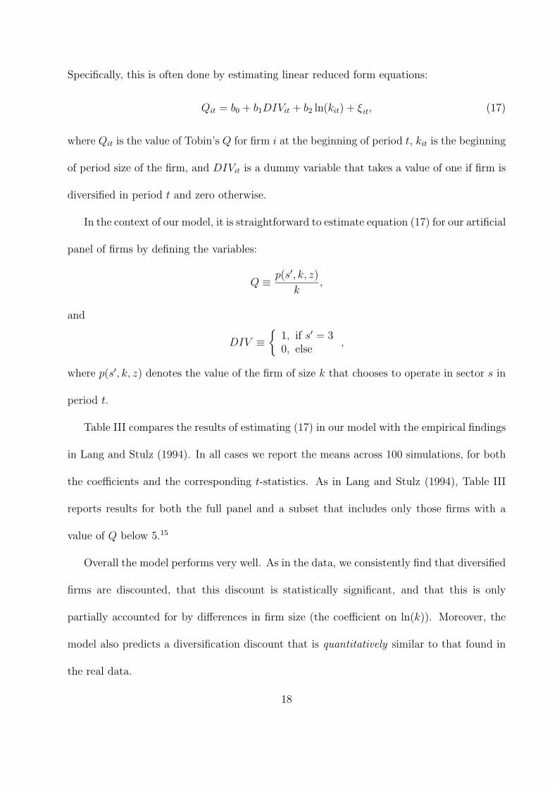
Specifically, this is often done by estimating linear reduced form equations:

Qit = b0 + b1DIVit + b2 ln(kit) + ξit, (17)

where Qit is the value of Tobin’s Q for firm i at the beginning of period t, kit is the beginning

of period size of the firm, and DIVit is a dummy variable that takes a value of one if firm is

diversified in period t and zero otherwise.

In the context of our model, it is straightforward to estimate equation (17) for our artificial

panel of firms by defining the variables:

Q ≡ p(s′, k, z)

k,

and

DIV ≡{

1, if s′ = 30, else

,

where p(s′, k, z) denotes the value of the firm of size k that chooses to operate in sector s in

period t.

Table III compares the results of estimating (17) in our model with the empirical findings

in Lang and Stulz (1994). In all cases we report the means across 100 simulations, for both

the coefficients and the corresponding t-statistics. As in Lang and Stulz (1994), Table III

reports results for both the full panel and a subset that includes only those firms with a

value of Q below 5.15

Overall the model performs very well. As in the data, we consistently find that diversified

firms are discounted, that this discount is statistically significant, and that this is only

partially accounted for by differences in firm size (the coefficient on ln(k)). Moreover, the

model also predicts a diversification discount that is quantitatively similar to that found in

the real data.

18

Looking only at the subset of firms with a value of Q below 5 shows that the observed

diversification discount is not due to a small number of outliers. Table III confirms that in

the model, as in the data, eliminating outliers does decrease the discount’s magnitude but

it does not eliminate it. Although smaller, the coefficient on the diversification dummy is

significant, both statistically and economically.

Thus, despite the fact that conglomerates operate efficiently and that diversification

clearly adds value to the firm, our model is able to rationalize the documented diversification

“discount”. Moreover, this discount also seems to possess the same robustness properties

that are observed in the actual data. Since diversification is optimal however, the explanation

cannot be that conglomerates destroy value. Instead, the success of the model hinges on the

endogenous selection mechanism identified in section A.4.

It is important to note that our results accord with the view that conglomerates are

indeed less efficient firms. Crucially however, they are not inefficient. In particular, and as

long as λ > 0, separation of their units destroys shareholder value.

Finally, the exact magnitude of the discount depends on synergies created by the

conglomerate, measured by the parameter λ. Indeed, if these synergies are too large, the

discount may disappear altogether. We view this dependence as an important strength of

the model and a useful direction for future research. For instance, allowing λ to vary across

firms could rationalize recent evidence suggesting that the magnitude of the discount seems

to vary with the level of synergies created by diversification (for example Chevalier (2001)).

19

B.1 Source of the Diversification Discount

Following Lang and Stulz (1994), Tables IV and V attempt to shed light on the source of the

discount. We focus on two subsamples of the full panel of firms: on-going conglomerates and

newly diversified firms. Table IV reports the results of estimating (17) for the subsample

of firms that do not change the number of segments in which they operate. Specifically,

we consider only the set of firms for which st = st−1 = ... = st−4, thus excluding all newly

diversified (as well as refocused) firms from the sample. As Table IV documents, however,

excluding these newly diversified firms does not eliminate the observed discount both in the

data and in the model. Moreover, the actual value of the discount in our model is again very

close to that observed by Lang and Stulz (1994).

By contrast, Table V looks at the behavior of firms that change the numbers of segments

of activity across adjacent years. Specifically, these firms are classified as “diversifying”, if

they change the number of sectors they operate in from one to two (formally st−1 = 1 or 2

and st = 3) and “focusing” firms if they reduce the number of activities from 2 to 1 (st−1 = 3

and st = 1 or 2). These firms are then compared with those that maintained the number of

activities constant during the same period. For “diversifying” firms, the comparison group is

the set of other previously focused firms that chose not to become diversified in the current

period. Similarly, focusing firms are compared with other diversified firms that chose to

remain diversified.

Following Lang and Stulz (1994) we report two alternative results. First, we look at the

average differences in Q at the time that the firms choose to expand (or contract). Next, we

also look at the dynamic effects of the decision, by comparing the effects of diversification

20

(refocusing) on ∆Q.

The findings are somewhat inconclusive, both in the model and in the data since no

coefficient seems statistically significant.16 Nevertheless there is some suggestion, both in the

model and the data, that diversifying firms seem to experience drops in Q (while the opposite

happens for focusing firms). The model’s implications for the level of Q are somewhat less

successful, but not statistically significant.

In recent empirical work Burch and Nanda (2003), and Dittmar and Shivdasani (2003)

also find that firm spin-offs and divestures tend to raise value, while improving the quality

of investment. The results in Table V show that their evidence is also consistent with an

optimal allocation of resources by firms. Intuitively this occurs because, firms in our model

will refocus when productivity shocks become more asymmetric. Thus, divestitures are also

going to be associated with increases in productivity and investment in on-going activities.

Overall, Tables IV and V broadly confirm the empirical success of our model. It is not

only capable of generating a diversification discount, but also provides quantitatively realistic

results for the subsets of existing and newly diversified firms.

B.2 Robustness

While our benchmark calibration appears quite successful it is interesting to examine the

robustness of our findings to alternative choices of parameter values, particularly in light

of the fact that there is relatively little a-priori evidence for the four parameters, f ,λ,

σ, and ρ. Table III investigates whether our main findings, regarding the existence of a

diversification discount, are sensitive to our choices for these parameters. Specifically, Table

VI compares the results of fitting the regression equation (17) to artificial samples, generated

21

by varying our choices for the key parameters f ,λ, σ, and ρ. While the exact magnitude

of the discount varies across the different experiments, the basic qualitative finding of a

diversification discount seems robust. The alternative values are chosen to indicate which

changes lead to lower discounts. Thus, low variability in productivity (low σ or ρ) reduces

the cross-sectional variability in Q and thus the discount. High fixed costs, f , increase the

cost savings of conglomerates, λf , and lower the discount. Decreasing the cost savings λ

also lowers the implied discount. The reason is that lower synergies make diversification less

attractive. With a low λ most conglomerates are formed to take advantage of decreasing

returns to scale, and this effect is entirely captured by the large coefficient of ln k.

C Diversification and Productivity

In our model productivity differentials play a key role in determining firm behavior and

the observed link between diversification and firm valuation. In this section, we investigate

whether the implied movements in firm and sectoral productivity are also consistent with

existing empirical evidence. In a recent study, Schoar (2002) carefully documents the

productivity patterns in manufacturing using the LRD database. Specifically, she computes

Total Factor Productivity (TFP) for each plant, j, in each firm, i, and every period, t, by

estimating the residual, εijt, in the following log-linear Cobb-Douglas production function:

ln(yijt) = ajt + bjt ln (kijt) + cjt ln (lijt) + εijt, (18)

Given this measure of productivity, we can examine the relation between firm

diversification and firm productivity. Schoar (2002) focuses on two measures. First, she

seeks to capture static differences in average productivity across firms by estimating the

22

following equation:

TFPijt = a1 + b1 × SEGit + µijt. (19)

where SEGit is the logarithm of the number of segments in which firm i operates in period

t. Thus, estimating b1 > 0 implies that diversified (multi-segment) firms are, on average,

more productive than focused firms. In addition, she also examines the dynamic effects of

diversification on future productivity. This is accomplished by estimating the equation:

TFPijt = a2 + b2 × AFTERit + νijt. (20)

where AFTERit is defined as a dummy variable that equals one in the period after the

firm diversifies and it is equal to zero otherwise.17 Thus, a finding of b2 > 0 implies that

diversification improves plant productivity.

It is again relatively straightforward to use the artificial panel of firms generated by our

model to replicate Schoar’s (2002) procedures and compare the results. Given our measures

of capital, labor and output and assuming that each activity corresponds to one plant we

can easily estimate (18-20). Table VII compares our findings with the results in Tables II

and IV from Schoar (2002).

While Schoar (2002) finds a significant productivity premium of more than 3% for

diversified firms, our model implies that focused firms are, on average, 2.3% more productive.

However, this result depends on the magnitude of the diversification discount, since lower

productivity leads to lower valuations. This is important since in Schoar’s LRD sample the

average market discount for diversified firms is only about 10%, while our model, which is

calibrated to replicate the Lang and Stulz’s (1994) results, implies a discount of about 20%.

23

The last column of Table VII addresses this issue by recalibrating our model to generate a

discount of exactly 10%, thus making our results directly comparable with hers. We find that

in this case our model can also match the observed productivity premium for conglomerates.

Table VII also shows that our model successfully reproduces the observed losses of

productivity after the firm diversifies.18 As Schoar (2002) argues, these findings reinforce the

importance of distinguishing between the static effect of being diversified and the dynamic

effect of becoming diversified. From a static, or cross-sectional, point-of-view, diversified

firms are, on average, more productive than focused firms. However, as Figure 1 illustrates,

diversification in our model is often the result of bad productivity shocks in on-going

activities. Thus, it is not surprising to find that, on average, diversification is associated

with productivity losses in incumbent sectors, just as Schoar (2002) finds.19

These results suggest that our basic argument that diversification decisions are driven

by efficient responses to productivity differentials is not the result of assuming unrealistic

patterns for productivity. The fact that our model is consistent with much of the evidence

also suggests a possible alternative interpretation to the more popular “new toy effect”,

that emphasizes a shift in focus by managers towards the newly acquired segments at the

expense of incumbent ones. Our findings show that this evidence can also be rationalized in

the context of a value maximizing model.

III Conclusions

In this paper we show that a general dynamic model of optimal behavior of a firm that

maximizes shareholder value is actually consistent with the main empirical findings about

firm diversification and performance. In our model, diversification is a natural result of firm

24

growth and it stems from dynamic firm strategies that maximize value. Diversification allows

a firm to explore new productive opportunities while taking advantage of synergies.

The dynamic structure of our model allows us to examine several aspects of the

relationship between firm diversification and performance in a very general setting. In

particular, we need not place any significant restrictions on the nature of functional forms

or parameter values in our model, beyond those already discussed. The very forces leading

to optimal diversification, are sufficient to generate a wealth of realistic features, regarding

firm diversification, size, productivity and valuations.

We obtain several important results. First, we can show that firms currently expanding

are not only less productive than other (non-expanding) focused firms, but they also

experience productivity losses after the expansion, as documented by Schoar (2002). Second,

as Santalo (2001) and Maksimovic and Phillips (2002) suggest, we find that size differences

can account for part of the differences both in productivity and valuation across focused

and diversifying firms. However, we also show that this size “effect”, can not account for

all of these differences. Finally, and perhaps more surprisingly, we show that despite all

the obvious advantages to firm diversification and the fact that firm diversification does

not destroy value in our model, it is still possible to obtain a diversification discount as

documented by Lang and Stulz (1994).

25

References

[1] Amihud, Yakov, and Baruch Lev, 1981, Risk Reduction as a Managerial Motive for

Conglomerate Mergers, Bell Journal of Economics 12, 605-617.

[2] Berger, Philip and Ofek, Eli, 1995, Diversification’s Effect on Firm Value, Journal of

Financial Economics 37, 39-65.

[3] Bernardo, Antonio and Chowdhry, Bhagwan 2002, Resources, Real Options and

Corporate Strategy, Journal of Financial Economics, forthcoming.

[4] Burch, Timothy, and Vikram Nanda, 2003, Divisional Diversity and the Conglomerate

Discount: The Evidence from Spin-Offs, forthcoming, Journal of Financial Economics

[5] Burnside, Craig, Production Function Regressions, Returns to Scale and Externalities,

Journal of Monetary Economics, vol 37, pp 177-201, 1996.

[6] Campa, Jose and Kedia, Simi, 2002, Explaining the Diversification Discount, Journal

of Finance, 57(4), 135-160.

[7] Chevalier, Judith 2001, Why Do Firms Undertake Diversifying Mergers? An

Examination of the Investment Policies of Merging Firms, unpublished manuscript,

University of Chicago.

[8] Cocco, Joao and Jan Mahrt-Smith, 2001, Return Sensitivity to Industry Shocks:

Evidence on the (In)-Efficient Use of Internal capital Markets, unpublished manuscript,

London Business School.

26

[9] Dennis, Dabid, Dennis, Dianne and Sarin, Atulya, Agency Problems, Equity Ownership

and Corporate Diversification, Journal of Finance, 52(1), 135-160.

[10] Dittmar, Amy and Anil Shivdasani, 2003, Divestitures and Divisional Investment

Policies, forthcoming, Journal of Finance.

[11] Gomes, Joao, 2001, Financing Investment, American Economic Review, 91(5), 1263-

1285.

[12] Graham, John, Lemmon, Michael and Wolf, Jack, 2002, Does Corporate Diversification

Destroys Value?, Journal of Finance 57, 695-720.

[13] Hopenhayn, Hugo, 1991,Entry, Exit, and Firm Dynamics In Long Run Equilibrium,

Econometrica, 60(5), 1127–1150.

[14] Jensen, Michael, 1986, Agency Costs of Free Cash Flow, Corporate Finance, and

Takeovers, American Economic Review 76(2), 323-329.

[15] Jensen, Michael, and Kevin Murphy, 1990, Performance Pay and Top Management

Incentives, Journal of Political Economy 98, 225-264

[16] Lamont, Owen and Polk, Chistopher 2001, The Diversification Discount: Cash Flows

Versus Returns, Journal of Finance, 56(5), 1693-1721.

[17] Lamont, Owen and Polk, Chistopher 2002, Does Diversification Destroys Value?

Evidence from Industry Shocks, Journal of Financial Economics vol. 63(1)

[18] Lang, Larry and Rene Stulz, 1994, Tobin’s q,Corporate Diversification, and Firm

Performance, Journal of Political Economy 102(6) 1248-1280.

27

[19] Maksimovic, Vojislav and Phillips, Gordon, 2002, Do Conglomerate Firms Allocate

Resources Inefficiently Across Industries, forthcoming, Journal of Finance.

[20] Matsusaka, John, 2001, Corporate Diversification, Value Maximization, and

Organizational Capabilities, Journal of Business 74(3), 409-431.

[21] Inderst, Roman and Muller, Holger, 2003, Internal vs. External Financing: An Optimal

Contracting Approach, forthcoming, Journal of finance.

[22] Rajan, Raghuram, Servaes, Henri, and Zingales, Luigi, 2000, The Cost of Diversity:

The Diversification Discount and Inefficient Investment, Journal of Finance 55, 35-80.

[23] Santalo, Juan, 2001, Diversification Discount, Size Discount and Organizational Capital,

unpublished manuscript, University of Chicago.

[24] Scharfestein, David, and Stein, Jeremy 2000, The Dark Side of Internal Capital Markets

I, Journal of Finance 55, 2537-2564.

[25] Schleifer, Andrei, and Robert Vishny, 1989, Managerial Entrenchment, The Case of

Manager-Specific Investment, Journal of Financial Economics 25, 123-139.

[26] Schoar, Antoinette, 2002, Effects of Corporate Diversification on Productivity,

forthcoming, Journal of Finance.

[27] Stokey, Nancy and Lucas, Robert, 1989, Recursive Methods in Economic Dynamics,

Harvard University Press.

[28] Stulz, Rene, 1990, Managerial Discretion and Optimal Financing Policies, Journal of

Financial Economics 26, 3-27.

28

[29] Villalonga, Belen, 2001, Does Diversification Cause the “Diversification Discount”?,

unpublished manuscript, Harvard University.

[30] Wernerfelt, Birger and Cynthia A. Montgomery, 1988, Tobin’s q and Importance of

Focus in Firm Performance, American Economic Review 78, 246-250

[31] Whited, Toni, 2001, Is It Inefficient Investment That Causes Diversification Discount?,

Journal of Finance 56, 1667-1691.

29

Notes

1See Wernerfelt and Montgomery (1988), Lang and Stulz (1994), Berger and Ofek (1995), Rajan, Servaes,

and Zingales (2000), Whited (2001), Lamont and Polk (2001, 2002), and among others.

2See Jensen (1986), Amihud and Levy (1981), Jensen and Murphy (1990), Shleifer and Vishny (1989),

and Stulz (1990), Denis, Denis and Sarin (1997), and Scharfestein and Stein (2000) among others.

3Although we do not address their findings, recent work by Whited (2002), Graham, Lemmon and Wolf

(2002), also suggests that the diversification discount is not caused inefficient conglomerates

4This assumption has little impact on our numerical analysis. It will, however, make it easier to construct

Figure 2 below and to gain some intuition about our results. A more realistic model would allow for some

form of costly switching, possibly as a consequence of learning or irreversible investment, but this would

greatly complicate our analysis.

5Fixed costs guarantee a minimum scale of production, thus forcing a firm to stay focused, unless outside

opportunities are sufficiently attractive. As we show below, without fixed costs a firm will always be

diversified.

6Since both output elasticities and prices do not differ across sectors, capital-labor ratios must also be

identical. It follows that the conglomerate must allocate the same share of capital and labor inputs to each

sector.

7We use the convention s′, k′, z′, etc. to denote the value of the state variables that are relevant at the

beginning of the next period.

8Formally, this threshold is a separating hyperplane in the 4-dimensional space of state variables.

9This endogenous relation between productivity and diversification is also present in Maksimovic and

Phillips (2002) and Inderst and Muller (2003). Our dynamic setting however allows us to also account for

the interaction between productivity and firm size as joint determinants of the decision to diversify. As we

will see this allows us to better account for the existing empirical evidence.

10This problem is equivalent to that of a shareholder investing in the stocks of each firm (Gomes (2001)).

11Note that π(s′, k, z;W ) = π(s(s, k, z), k, z;W ) = π(s, k, z;W ). Similarly, for l(s, k, z;W ) = l(s′, k, z;W ).

12The proof follows the arguments provided in Hopenhayn (1992) and Gomes (2001).

13The preference parameters are not important and we simply use β = 1/1.065 and A = W = 0.5.

14The use of Tobin’s Q to measure the value of the firm is theoretically correct even in the presence of

measurement error

15When possible we focus on the numbers reported by Lang and Stulz (1994) for “industry-adjusted” Q′s,

since these control for the fact that diversified firms are generally concentrated in low Q industries.

30

16Intuitively, the lack of statistical significance in the artificial sample is a consequence of the small variation

in the shocks z. Although large variations would change this quantitative finding, a larger dispersion in z

would lead to an unrealistically high dispersion in Q.

17Schoar (2002) also adds variables such as age and the number of segments the firm operates. In the

context of our model, however, age is not defined and the number of segments is redundant.

18Here, our results can only be compared with Schoar’s (2002) estimates for incumbent plants since, in

our model, new plants have no prior history.

19Firms may also diversify if the diversification threshold moves because outside opportunities improve.

In this case productivity in the incumbent sector need not fall for these firms.

31

Appendix

A. Proofs

We derive all formal proofs under the most general set of conditions. Accordingly, define the

set S = {1, 2, 3}. Let K × L ⊆ R2+ be the space of inputs and suppose that the stochastic

process for the shock has a bounded support Z = [z, z]×[z, z], −∞ < z < z < ∞. Moreover,

define z and k as the minimal sigma-fields generated by Z and K, respectively. Finally

let F (k, l) denote a general decreasing returns to scale technology and Q(zt+1|zt) be the

transition function of z.

We make the following minimal assumptions regarding the nature of these functions and

the size of the fixed costs.

Assumption 1 The production function F (•): (i) is continuously differentiable; (ii) is

strictly increasing; (iii) is strictly concave; (iv) satisfies the standard Inada conditions; and

(v) exhibits decreasing returns to scale in k and l.

Assumption 2 The technology levels zt = (z1t , z

2t ) follow a joint Markov transition function

Q(zt+1, zt) : Z ×z → [0, 1]× [0, 1] that: (i) is stationary, (ii) is monotone and (iii) satisfies

the Feller property. Let G(z) denote the invariant distribution of z.

Assumption 3 The fixed costs of production, f, are not too large, i.e. ∃k ∈ R+ : f ≤

zF (k, l).

32

A.1 Proof of Proposition 1

To show existence and uniqueness define the operator

(Tv)(s, k, z) = max{k′,s′}

{π(s′, k, z) + (1 − δ)k − k′ + β

∫v(s′, k′, z′)Q(dz′, z)

}, (A1)

s′ ∈{ {s, 3}, s = 1, 2

S, s = 3.

Let C(S × K × Z) be the space of all bounded and continuous functions in S × K × Z.

The proof is in two steps:

(a) T : C(S × K × Z) −→ C(S × K × Z) (Lemma 6);

(b) T is a contraction in C(S × K × Z) (Lemma 7).

The Contraction Mapping Theorem then guarantees that there is a unique fixed point

that satisfies (A1).

Monotonicity then follows immediately from Theorems 9.7 and 9.11 in Stokey and Lucas

(1989).

Lemma 6 T : C(S × K × Z) −→ C(S × K × Z) .

Proof. Suppose v(s′, k′, z′) ∈ C(S × K × Z). Since Q(dz′|z) has the Feller property it

follows from Lemma 9.5 in Stokey and Lucas (89) that

∫v(s′, k′, z′)Q(dz′, z) ∈ C(S × K × Z).

Since π(s′, k, z) is also bounded and continuous, the result follows immediately.

Lemma 7 T is a contraction in C(S × K × Z).

Proof. The proof uses Blackwell’s sufficient conditions for a contraction.

33

(a)Monotonicity.

Consider v1(s, k, z), v2(s, k, z) ∈ C(S × K × Z), such that v1(s, k, z) ≥ v2(s, k, z). It

follows that ∫v1(s

′, k′, z′)Q(dz′, z) ≥∫

v2(s′, k′, z′)Q(dz′, z),

and hence

(Tv1)(s, k, z) ≥ (Tv2)(s, k, z).

(b) Discounting

Let a ∈ R and v(s, k, z) ∈ C(S × K × Z). It follows that

(Tv + a)(s, k, z) = v(s, k, z) + βa = (Tv)(s, k, z) + βa.

A.2 Proof of Proposition 2

Using (8) we can rewrite the optimal diversification decision of a focused firm as

Π(s, k, z) + Ψ(s, z) ≥ (1 − λ)f, s ∈ {1, 2} (A2)

where

Π(s, k, z) ≡ π(3, k, z) − π(s, k, z) + (1 − λ)f, (A3)

and

Ψ(s, z) = Ψ(s′, z) |s′=s≡ maxk′

{β

∫v(3, k′, z′)Q(dz′, z) − k′

}−

−maxk′

{β

∫v(s, k′, z′)Q(dz′, z) − k′

}. (A4)

Equation (A2) decomposes the optimal diversification decision into a “profit” component,

Π(s, k, z), and an “option” component, Ψ(s, z), associated with the continuation payoffs. By

34

definition k(s, z), satisfies

Π(s, k(s, z), z) + Ψ(s, z) = (1 − λ)f, ∀(s, z) ∈ S × Z (A5)

Lemmas 8 and 9 imply that the left hand side is non-negative and strictly increasing in k.

Hence, if diversification is optimal for k = k(s, z), it must also be optimal for k > k(s, z). If

the left hand side exceeds (1 − λ)f then diversification is always optimal and k(s, z) = 0.

To establish monotonicity let z = (zs, zs) and z = (zs +∆zs, zs), with ∆zs > 0. It follows

from (A5) that

Π(s, k(s, z), z) + Ψ(s, z) = (1 − λ)f.

Lemmas 8 and 9 imply that both Π(·) and Ψ(·) are decreasing in zs. Since Π(·) is increasing

in k, it follows that k(s, z) > k(s, z).

Analogously, let z = (zs, zs+∆zs), with ∆zs > 0. Since both Π(·) and Ψ(·) are increasing

in zs (Lemmas 8 and 9), it follows that k(s, z) < k(s, z).

Now consider a previously diversified firm. Here the threshold is determined by

p(3, k(s, z), z) ≥ max{

p(1, k(s, z), z), p(2, k(s, z), z)}

(A6)

or, simply, by

mins∈{1,2}

{Π(s, k(s, z), z) + Ψ(s, z)

}= (1 − λ)f, ∀z ∈ Z (A7)

Again the left hand side is non-negative and strictly increasing in k, since Π(s, k, z)+Ψ(s, z)

has these properties as well, and the result follows as above.

Lemma 8 Let Π(s, k, z) be defined by (A3). Then Π(s, k, z) is (i) non-negative; (ii) weakly

increasing in k; and (iii) decreasing in zs and increasing in zs, s �= s.

35

Proof. (i) Π(s, k, z) ≥ 0. By definition

π(3, k, z) = π(1, θ∗k, z) + π(2, (1 − θ∗)k, z) + λf

where θ∗ = θ(k, z), is the optimal share of capital allocated to sector 1. Clearly then

π(3, k, z) ≡{

π(1, k, z) − (1 − λ)f,π(2, k, z) − (1 − λ)f,

θ∗ = 1θ∗ = 0

since θ∗ is chosen optimally, it follows that

Π(s, k, z) = π(3, k, z) − π(s, k, z) ≥ 0

(ii) Monotonicity in k. Taking derivatives of π(3, k, z) with respect to k we obtain

∂π(3, k, z)

∂k=

∂π(1, θ∗k, z)

∂(θk)

(k∂θ∗

∂k+ θ∗

)+

∂π(2, (1 − θ∗)k, z)

∂(θk)

(−k

∂θ∗

∂k+ (1 − θ∗)

)

Noting that the optimal choice of θ∗ implies

∂π(1, θ∗k, z)

∂(θk)=

∂π(2, (1 − θ∗)k, z)

∂(θk),

we immediately obtain

∂π(3, k, z)

∂k=

∂π(s′, θ∗k, z)

∂(θk)≥ ∂π(s, k, z)

∂k, s = 1, 2.

Where the inequality follows from the fact that the profit function is strictly concave and

θ ≤ 1. Since

∂Π(s, k, z)

∂k=

∂π(3, k, z)

∂k− ∂π(s, k, z)

∂k≥ 0, s = 1, 2

(iii) Monotonicity in z. Taking derivatives of π(3, k, z) with respect to zs and simplifying as

in (ii) we obtain

∂π(3, k, z)

∂zs=

∂π(s, θ∗k, z)

∂zs+

∂π(s, (1 − θ∗)k, z)

∂zs=

∂π(s, θ∗k, z)

∂zs

36

since production in sector s does not depend on the shock to sector i. Now, using the

envelope theorem and the profits definitions (6) and (5) yields

∂π(3, k, z)

∂zs= F (θ∗ks, ·) ≤ F (ks, ·) =

∂π(s, k, z)

∂zs.

and hence that

∂Π(s, k, z)

∂zs≤ 0, s = 1, 2.

Monotonicity in zs follows immediately from the fact that π(s, k, z) depends only on zs.

Lemma 9 Let Ψ(s, z) be defined by (A4). Then Ψ(s, z) is: (i) non-negative; and (ii)

decreasing in zs and increasing in zs, s �= s.

Proof. (i) Ψ(s, z) ≥ 0. First note that

v(3, k′, z′) = max {p(1, k′, z′), p(2, k′, z′), p(3, k′, z′)}

≥ max {p(s′′, k′, z′), p(3, k′, z′)} = v(s′, k′, z′),

∀(k′, z′) ∈ K × Z,∀s′′ ∈ {1, 2},

From monotonicity of Q(·) it follows that

∫max {p(1, k′, z′), p(2, k′, z′), p(3, k′, z′)}Q(dz′, z)

≥∫

max {p(s′′, k′, z′), p(3, k′, z′)}Q(dz′, z),

Hence for any value of z ∈ Z and any value of k′ ∈ K

β

∫v(3, k′, z′)Q(dz′, z) − k′ ≥ β

∫v(s′, k′, z′)Q(dz′, z) − k′.

Since this holds for every value of k′ it follows that it holds at the maximum and Ψ(s, z) ≥ 0.

37

(ii) Ψ(s, z) is decreasing in zs and increasing in zs, s �= s. Suppose zs >> zs. Then

p(s, k, z) >> p(s, k, z),

and consequently

v(3, k, z) ≈ max {p(s, k, z), p(3, k, z)} .

Given the monotonicity of Q(·) it follows that:

∫v(3, k′, z′)Q(dz′, z) ≈

∫max {p(s, k′, z′), p(3, k′, z′)}Q(dz′, z) =

∫v(s, k′, z′)Q(dz′, z),

and, therefore, Ψ(s, z) = 0.

Now suppose that the opposite is true, i.e. zs << zs. In that case

v(3, k, z) ≈ max {p(s, k, z), p(3, k, z)}

and

∫v(3, k′, z′)Q(dz′, z) ≈

∫max {p(s, k′, z′), p(3, k′, z′)}Q(dz′, z) >

∫v(s, k′, z′)Q(dz′, z).

which implies that Ψ(s, z) > 0. It follows from continuity of both v(·) and Q(·) that Ψ(s, z)

must fall with zs.

An identical argument can be constructed to establish that Ψ(s, z) increases with zs.

A.3 Proof of Corollary 3

In the absence of fixed costs inequality (A2) is always satisfied.

A.4 Proof of Corollary 4

Inequality (A2) is always satisfied if λ ≥ 1.

38

B. Solution Method

The computational strategy involves the following steps

1. Solving the Bellman Equation (7) and computing the optimal firm decision rules;

2. Using the optimal decision rules to iterate on (12) and compute the stationary measure

µ = µ′ = µ∗

3. Computing aggregate quantities and using the market clearing condition (15) to

determine the equilibrium levels of consumption and labor.

Given the properties of our problem, the first step is better implemented with the less

efficient but more robust method of value function iteration on a discrete state space.

We specify a grid with a finite number of points for the capital stock as well as a finite

approximation to the normal random vector z. The later task is accomplished using in

Tauchen and Hussey’s (1991) method for optimal discrete state space approximations to

normal random variables. We use 15 × 15 grid points for this procedure. The space for

the capital stock is divided in 201 equally spaced elements. In either case the results were

relatively unchanged when we use finer grids. The upper bound for capacity, k, was chosen

to be non-binding at all times.

To compute µ∗, we take the optimal value function v(s, k, z) and the decision rules

k(s, k, z) and s(s, k, z), as well as the stochastic process for the technology shocks z and

proceed as follows:

• Define the size of the panel data, by specifying the number of firms M and the length

of time T.

39

• Simulate a sequence of exogenous technology shocks zit = (z1it, z

2it) for each firm i in

every period t.

• For the initial period

(i) Initiate each firm’s capital stock at k = k0.

(ii) Start the simulation by using draws from a uniform distribution to randomly

allocating firms to either sector 1 or 2.

• For all other periods

(i) Given the current state for each firm i, (sit−1, kit, zit) use the optimal policy functions

to determine next period’s capital stock, kit+1, and sectoral decision, sit.

(ii) Using the value function, compute the current market value of the firm i, vit.

(iii) Using the stochastic process for z, compute next period’s shock zit+1.

(v) Construct the cross-sectional distribution of firms µit = µ(sit, kit, zit).

• Continue the simulation until∣∣∣∣µit − µit+1

∣∣∣∣ < ε.

Using the stationary distribution, µ, it is straightforward to use the goods market

condition to obtain aggregate consumption.

40

Figure 1: Timing of Events

t t+1�

�

Firm arrives with(st−1, kt, zt−1)

�

zt is revealed

�

Firm produces and choosesst and kt+1

41

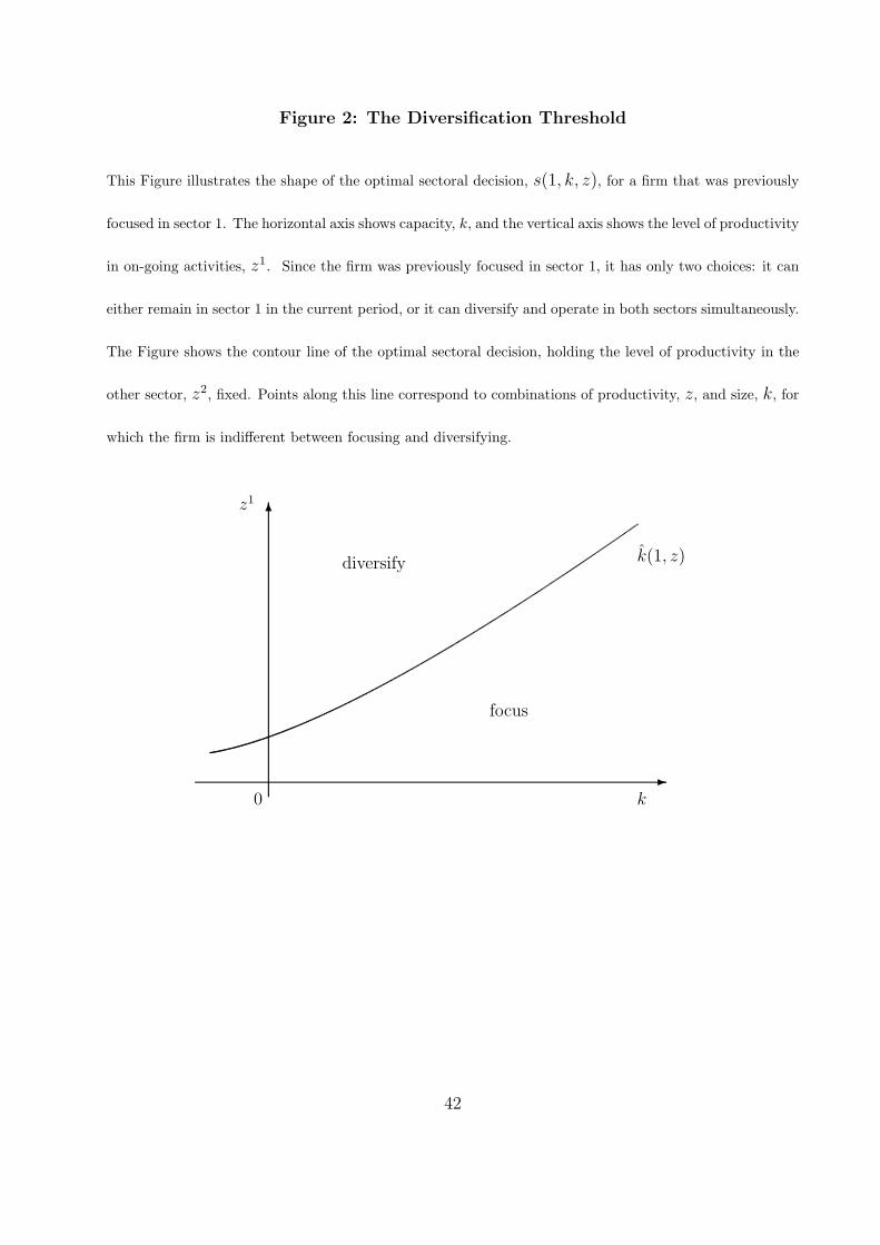
Figure 2: The Diversification Threshold

This Figure illustrates the shape of the optimal sectoral decision, s(1, k, z), for a firm that was previously

focused in sector 1. The horizontal axis shows capacity, k, and the vertical axis shows the level of productivity

in on-going activities, z1. Since the firm was previously focused in sector 1, it has only two choices: it can

either remain in sector 1 in the current period, or it can diversify and operate in both sectors simultaneously.

The Figure shows the contour line of the optimal sectoral decision, holding the level of productivity in the

other sector, z2, fixed. Points along this line correspond to combinations of productivity, z, and size, k, for

which the firm is indifferent between focusing and diversifying.

�k

focus

diversify

�z1

0

k(1, z)

42

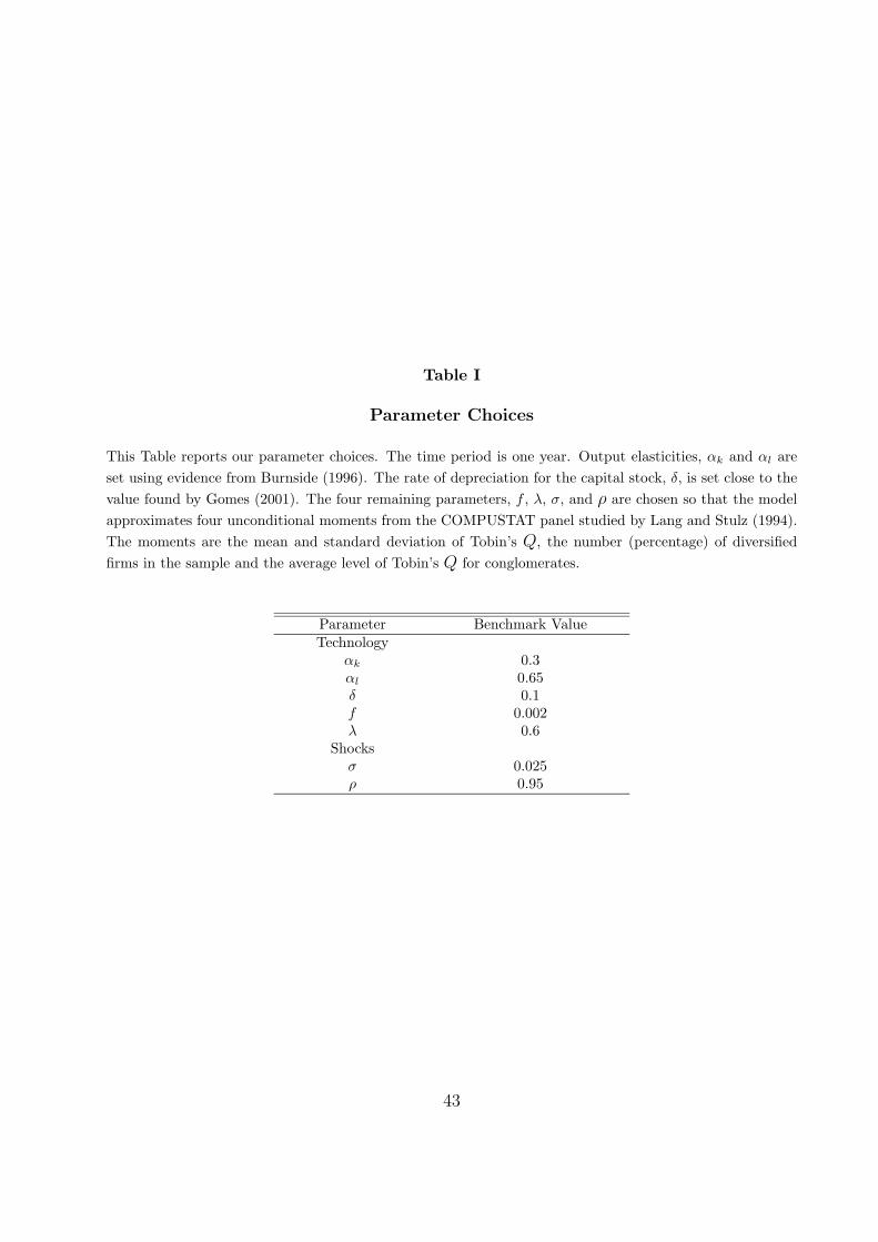
Table I

Parameter Choices

This Table reports our parameter choices. The time period is one year. Output elasticities, αk and αl areset using evidence from Burnside (1996). The rate of depreciation for the capital stock, δ, is set close to thevalue found by Gomes (2001). The four remaining parameters, f , λ, σ, and ρ are chosen so that the modelapproximates four unconditional moments from the COMPUSTAT panel studied by Lang and Stulz (1994).The moments are the mean and standard deviation of Tobin’s Q, the number (percentage) of diversifiedfirms in the sample and the average level of Tobin’s Q for conglomerates.

Parameter Benchmark ValueTechnology

αk 0.3αl 0.65δ 0.1f 0.002λ 0.6

Shocksσ 0.025ρ 0.95

43

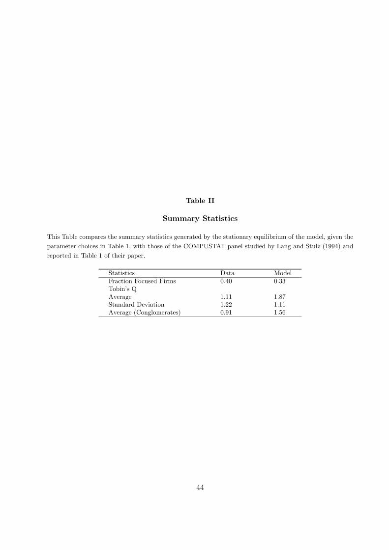
Table II

Summary Statistics

This Table compares the summary statistics generated by the stationary equilibrium of the model, given theparameter choices in Table 1, with those of the COMPUSTAT panel studied by Lang and Stulz (1994) andreported in Table 1 of their paper.

Statistics Data ModelFraction Focused Firms 0.40 0.33Tobin’s QAverage 1.11 1.87Standard Deviation 1.22 1.11Average (Conglomerates) 0.91 1.56

44

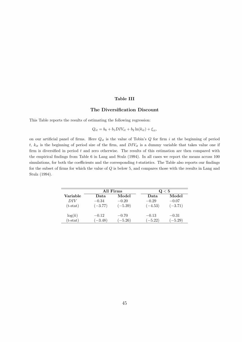
Table III

The Diversification Discount

This Table reports the results of estimating the following regression:

Qit = b0 + b1DIVit + b2 ln(kit) + ξit,

on our artificial panel of firms. Here Qit is the value of Tobin’s Q for firm i at the beginning of periodt, kit is the beginning of period size of the firm, and DIVit is a dummy variable that takes value one iffirm is diversified in period t and zero otherwise. The results of this estimation are then compared withthe empirical findings from Table 6 in Lang and Stulz (1994). In all cases we report the means across 100simulations, for both the coefficients and the corresponding t-statistics. The Table also reports our findingsfor the subset of firms for which the value of Q is below 5, and compares those with the results in Lang andStulz (1994).

All Firms Q < 5Variable Data Model Data Model

DIV(t-stat)

−0.34(−3.77)

−0.20(−5.39)

−0.29(−4.53)

−0.07(−3.71)

log(k)(t-stat)

−0.12(−3.48)

−0.70(−5.26)

−0.13(−5.22)

−0.31(−5.29)

45

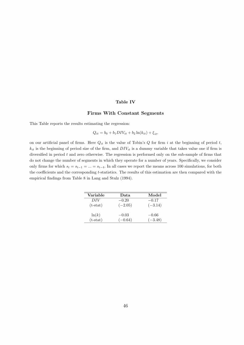
Table IV

Firms With Constant Segments

This Table reports the results estimating the regression:

Qit = b0 + b1DIVit + b2 ln(kit) + ξit,

on our artificial panel of firms. Here Qit is the value of Tobin’s Q for firm i at the beginning of period t,kit is the beginning of period size of the firm, and DIVit is a dummy variable that takes value one if firm isdiversified in period t and zero otherwise. The regression is performed only on the sub-sample of firms thatdo not change the number of segments in which they operate for a number of years. Specifically, we consideronly firms for which st = st−1 = ... = st−4. In all cases we report the means across 100 simulations, for boththe coefficients and the corresponding t-statistics. The results of this estimation are then compared with theempirical findings from Table 8 in Lang and Stulz (1994).

Variable Data ModelDIV

(t-stat)−0.20(−2.05)

−0.17(−3.14)

ln(k)(t-stat)

−0.03(−0.64)

−0.66(−3.48)

46

Table V

Firms Changing Segments

This Table compares firms that change the numbers of segments of activity across adjacent years with thosefirms that maintain the number of activities constant. Specifically, firms are classified as “diversifying” ifthey change the number of sectors they operate from one to two (formally st−1 = 1 or 2 and st = 3). Weprovide two separate results. First, we look at the average differences in Q at the time of the diversificationtakes place by estimating the regression:

Qit = b0 + b1DIVit + ξit,

for the subset of previously focused firms (st−1 < 3). Here Qit is the value of Tobin’s Q for firm i at thebeginning of period t, and DIVit is a dummy variable that takes value one if firm has been focused at t−1 andbecomes diversified in period t and zero otherwise. Next, we look at the dynamic effects of diversification, bycomparing the effects of diversification on ∆Q.˙We accomplish that by estimating the following regression:

∆Qit = b0 + b1DIVit + ξit,

again only for the subset of previously focused firms. Here ∆Qit = Qit −Qit−1. This Table also reports theeffects of refocusing on firm value, by estimating the same regressions as above, and letting DIVit equal oneif firm has been diversified at t − 1 and becomes focused in period t and zero otherwise. These regressionsare only estimated for the subset of previously diversified firms. In all cases we report the means across 100simulations, for both the coefficients and the corresponding t-statistics. The results of this estimation arethen compared with the empirical findings from Table 8 in Lang and Stulz (1994).

Regression on Qt Regression on ∆Qt = Qt+1 − Qt

Variable Data Model Data Model

Diversifying FirmsDIV

(t-stat)−0.163(−1.23)

0.045(0.37)

−0.204(−1.60)

−0.038(−1.46)

Focusing FirmsDIV

(t-stat)−0.016(−0.70)

0.035(1.40)

0.024(1.39)

0.020(1.22)

47

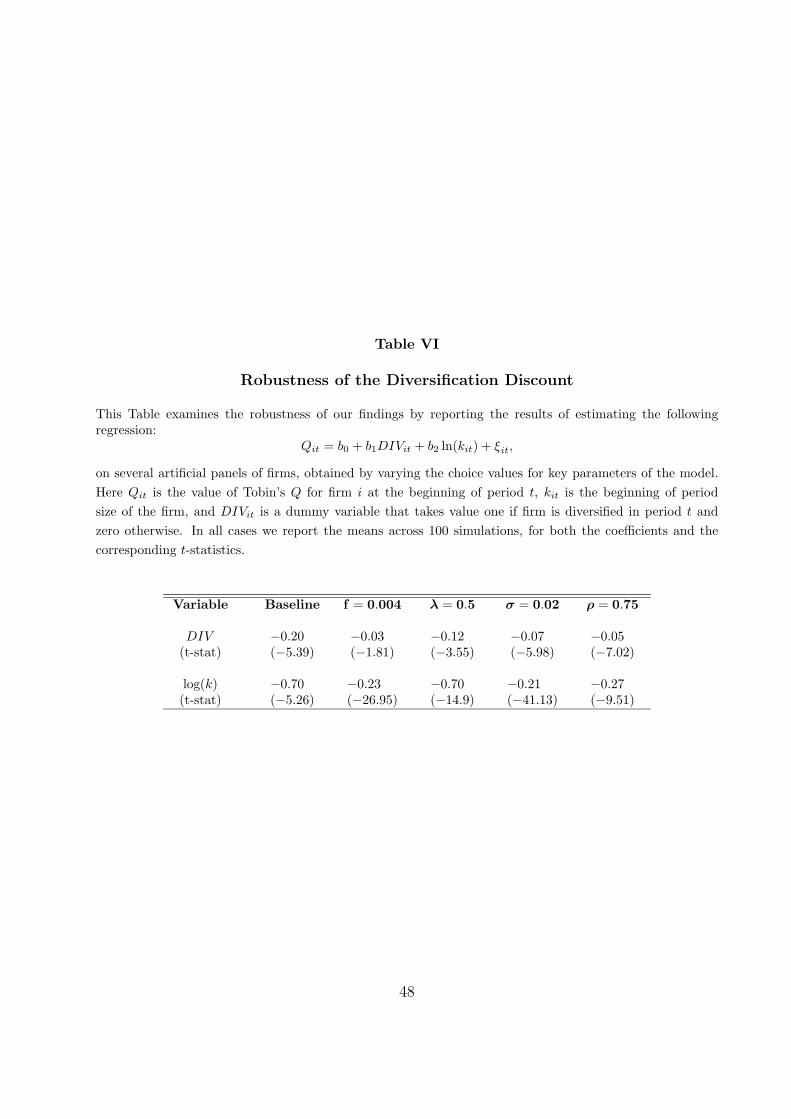
Table VI

Robustness of the Diversification Discount

This Table examines the robustness of our findings by reporting the results of estimating the followingregression:

Qit = b0 + b1DIVit + b2 ln(kit) + ξit,

on several artificial panels of firms, obtained by varying the choice values for key parameters of the model.Here Qit is the value of Tobin’s Q for firm i at the beginning of period t, kit is the beginning of periodsize of the firm, and DIVit is a dummy variable that takes value one if firm is diversified in period t andzero otherwise. In all cases we report the means across 100 simulations, for both the coefficients and thecorresponding t-statistics.

Variable Baseline f = 0.004 λ = 0.5 σ = 0.02 ρ = 0.75

DIV(t-stat)

−0.20(−5.39)

−0.03(−1.81)

−0.12(−3.55)

−0.07(−5.98)

−0.05(−7.02)

log(k)(t-stat)

−0.70(−5.26)

−0.23(−26.95)

−0.70(−14.9)

−0.21(−41.13)

−0.27(−9.51)

48

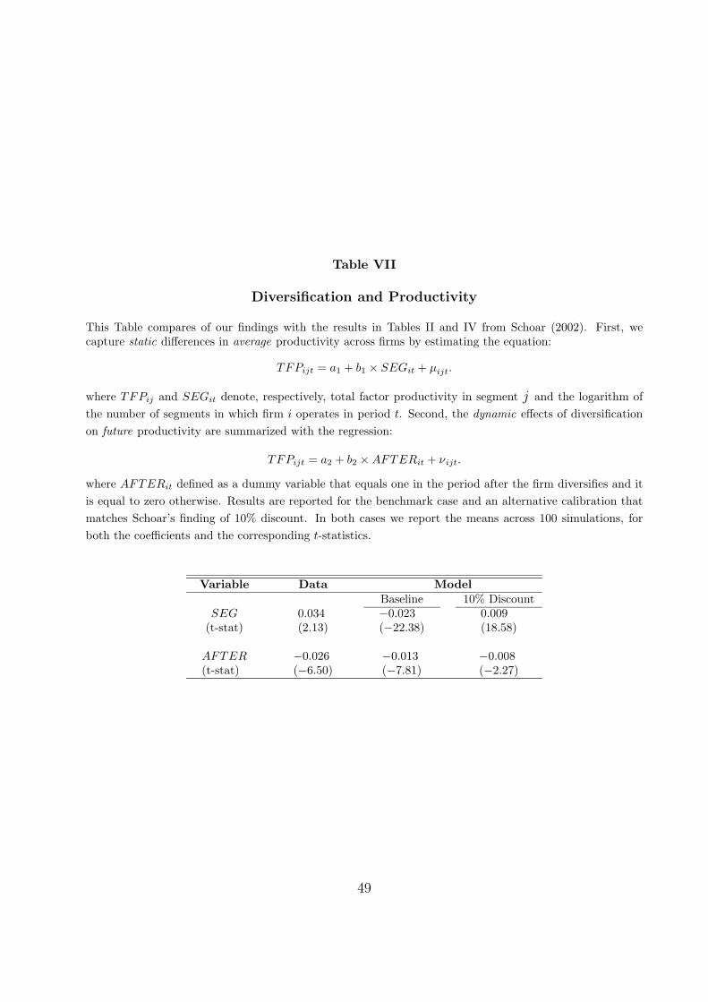
Table VII

Diversification and Productivity

This Table compares of our findings with the results in Tables II and IV from Schoar (2002). First, wecapture static differences in average productivity across firms by estimating the equation:

TFPijt = a1 + b1 × SEGit + µijt.

where TFPij and SEGit denote, respectively, total factor productivity in segment j and the logarithm ofthe number of segments in which firm i operates in period t. Second, the dynamic effects of diversificationon future productivity are summarized with the regression:

TFPijt = a2 + b2 × AFTERit + νijt.

where AFTERit defined as a dummy variable that equals one in the period after the firm diversifies and itis equal to zero otherwise. Results are reported for the benchmark case and an alternative calibration thatmatches Schoar’s finding of 10% discount. In both cases we report the means across 100 simulations, forboth the coefficients and the corresponding t-statistics.

Variable Data ModelBaseline 10% Discount

SEG(t-stat)

0.034(2.13)

−0.023(−22.38)

0.009(18.58)

AFTER(t-stat)

−0.026(−6.50)

−0.013(−7.81)

−0.008(−2.27)

49