Optimal distribution network reconfiguration using meta ...
114
University of Central Florida University of Central Florida STARS STARS Electronic Theses and Dissertations, 2004-2019 2015 Optimal distribution network reconfiguration using meta-heuristic Optimal distribution network reconfiguration using meta-heuristic algorithms algorithms Arash Asrari University of Central Florida Part of the Electrical and Electronics Commons Find similar works at: https://stars.library.ucf.edu/etd University of Central Florida Libraries http://library.ucf.edu This Doctoral Dissertation (Open Access) is brought to you for free and open access by STARS. It has been accepted for inclusion in Electronic Theses and Dissertations, 2004-2019 by an authorized administrator of STARS. For more information, please contact [email protected]. STARS Citation STARS Citation Asrari, Arash, "Optimal distribution network reconfiguration using meta-heuristic algorithms" (2015). Electronic Theses and Dissertations, 2004-2019. 52. https://stars.library.ucf.edu/etd/52
Transcript of Optimal distribution network reconfiguration using meta ...

University of Central Florida University of Central Florida
STARS STARS
Electronic Theses and Dissertations, 2004-2019
2015
Optimal distribution network reconfiguration using meta-heuristic Optimal distribution network reconfiguration using meta-heuristic
algorithms algorithms
Arash Asrari University of Central Florida
Part of the Electrical and Electronics Commons
Find similar works at: https://stars.library.ucf.edu/etd
University of Central Florida Libraries http://library.ucf.edu
This Doctoral Dissertation (Open Access) is brought to you for free and open access by STARS. It has been accepted
for inclusion in Electronic Theses and Dissertations, 2004-2019 by an authorized administrator of STARS. For more
information, please contact [email protected].
STARS Citation STARS Citation Asrari, Arash, "Optimal distribution network reconfiguration using meta-heuristic algorithms" (2015). Electronic Theses and Dissertations, 2004-2019. 52. https://stars.library.ucf.edu/etd/52
OPTIMAL DISTRIBUTION NETWORK RECONFIGURATION USING META-HEURISTIC ALGORITHMS
by
ARASH ASRARI B.S. Shahid Bahonar University of Kerman, Kerman, Iran, 2008
M.S. Ferdowsi University of Mashhad, Mashhad, Iran, 2012
A dissertation submitted in partial fulfillment of the requirements for the degree of Doctor of Philosophy
in the Department of Electrical Engineering & Computer Science in the College of Engineering and Computer Science
at the University of Central Florida Orlando, Florida
Spring Term 2015
Major Professor: Thomas Wu

© 2015 Arash Asrari
ii
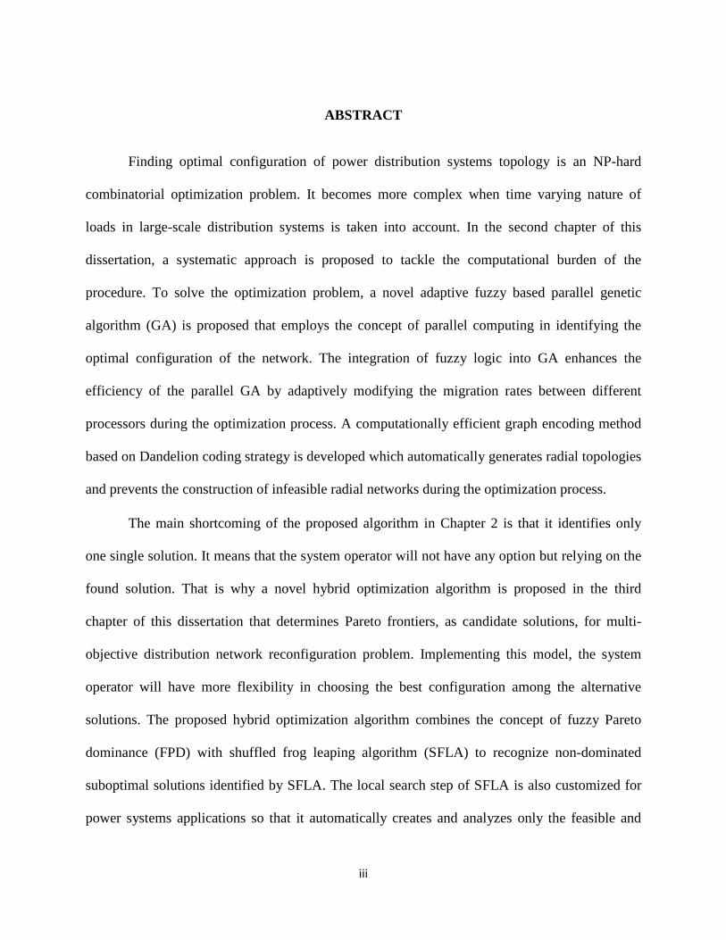
ABSTRACT
Finding optimal configuration of power distribution systems topology is an NP-hard
combinatorial optimization problem. It becomes more complex when time varying nature of
loads in large-scale distribution systems is taken into account. In the second chapter of this
dissertation, a systematic approach is proposed to tackle the computational burden of the
procedure. To solve the optimization problem, a novel adaptive fuzzy based parallel genetic
algorithm (GA) is proposed that employs the concept of parallel computing in identifying the
optimal configuration of the network. The integration of fuzzy logic into GA enhances the
efficiency of the parallel GA by adaptively modifying the migration rates between different
processors during the optimization process. A computationally efficient graph encoding method
based on Dandelion coding strategy is developed which automatically generates radial topologies
and prevents the construction of infeasible radial networks during the optimization process.
The main shortcoming of the proposed algorithm in Chapter 2 is that it identifies only
one single solution. It means that the system operator will not have any option but relying on the
found solution. That is why a novel hybrid optimization algorithm is proposed in the third
chapter of this dissertation that determines Pareto frontiers, as candidate solutions, for multi-
objective distribution network reconfiguration problem. Implementing this model, the system
operator will have more flexibility in choosing the best configuration among the alternative
solutions. The proposed hybrid optimization algorithm combines the concept of fuzzy Pareto
dominance (FPD) with shuffled frog leaping algorithm (SFLA) to recognize non-dominated
suboptimal solutions identified by SFLA. The local search step of SFLA is also customized for
power systems applications so that it automatically creates and analyzes only the feasible and
iii
radial configurations in its optimization procedure which significantly increases the convergence
speed of the algorithm.
In the fourth chapter, the problem of optimal network reconfiguration is solved for the
case in which the system operator is going to employ an optimization algorithm that is
automatically modifying its parameters during the optimization process. Defining three fuzzy
functions, the probability of crossover and mutation will be adaptively tuned as the algorithm
proceeds and the premature convergence will be avoided while the convergence speed of
identifying the optimal configuration will not decrease. This modified genetic algorithm is
considered a step towards making the parallel GA, presented in the second chapter of this
dissertation, more robust in avoiding from getting stuck in local optimums.
In the fifth chapter, the concentration will be on finding a potential smart grid solution to
more high-quality suboptimal configurations of distribution networks. This chapter is considered
an improvement for the third chapter of this dissertation for two reasons: (1) A fuzzy logic is
used in the partitioning step of SFLA to improve the proposed optimization algorithm and to
yield more accurate classification of frogs. (2) The problem of system reconfiguration is solved
considering the presence of distributed generation (DG) units in the network. In order to study
the new paradigm of integrating smart grids into power systems, it will be analyzed how the
quality of suboptimal solutions can be affected when DG units are continuously added to the
distribution network.
The heuristic optimization algorithm which is proposed in Chapter 3 and is improved in
Chapter 5 is implemented on a smaller case study in Chapter 6 to demonstrate that the identified
solution through the optimization process is the same with the optimal solution found by an
exhaustive search.
iv

ACKNOWLEDGMENTS
I would like to express my deepest appreciation to my supervisor, Dr. Thomas Wu, and
my co-advisor, Dr. Saeed Lotfifard, for the patient mentorship they provided to me. Most
especially, I would like to thank them for their excellent guidance, caring, support, and giving
me the freedom to pursue my doctoral research in an excellent atmosphere under their
supervision. I have learned a lot by working with them which has helped me recognize better my
academic goals. Also, I would like to thank Dr. Michael Haralambous, Dr. Jennifer Pazour and
Dr. George Atia as my committee members for their helpful comments on my proposal and this
dissertation.
v
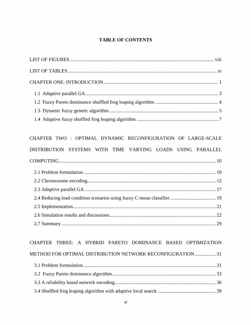
TABLE OF CONTENTS
LIST OF FIGURES ..................................................................................................................... viii
LIST OF TABLES ......................................................................................................................... xi
CHAPTER ONE: INTRODUCTION ............................................................................................. 1
1.1 Adaptive parallel GA ............................................................................................................ 3
1.2 Fuzzy Pareto dominance shuffled frog leaping algorithm ................................................... 4
1.3 Dynamic fuzzy genetic algorithm ........................................................................................ 5
1.4 Adaptive fuzzy shuffled frog leaping algorithm .................................................................. 7
CHAPTER TWO : OPTIMAL DYNAMIC RECONFIGURATION OF LARGE-SCALE
DISTRIBUTION SYSTEMS WITH TIME VARYING LOADS USING PARALLEL
COMPUTING ............................................................................................................................... 10
2.1 Problem formulation ........................................................................................................... 10
2.2 Chromosome encoding ........................................................................................................ 12
2.3 Adaptive parallel GA .......................................................................................................... 17
2.4 Reducing load condition scenarios using fuzzy C-mean classifier ..................................... 19
2.5 Implementation.................................................................................................................... 21
2.6 Simulation results and discussions ...................................................................................... 22
2.7 Summary ............................................................................................................................. 29
CHAPTER THREE: A HYBRID PARETO DOMINANCE BASED OPTIMIZATION
METHOD FOR OPTIMAL DISTRIBUTION NETWORK RECONFIGURATION ................. 31
3.1 Problem formulation ........................................................................................................... 31
3.2 Fuzzy Pareto dominance algorithm .................................................................................... 33
3.3 A reliability based network encoding.................................................................................. 36
3.4 Shuffled frog leaping algorithm with adaptive local search ............................................... 39
vi

3.5 Implementation.................................................................................................................... 45
3.6 Simulation results and discussions ...................................................................................... 47
3.7 Summary ............................................................................................................................. 55
CHAPTER FOUR: OPTIMAL DISTRIBUTION NETWORK RECONFIGURATION USING
DYNAMIC FUZZY BASED GENETIC ALGORITHM ............................................................ 56
4.1 Overview of genetic algorithm ............................................................................................ 56
4.2 Determining crossover and mutation parameters ................................................................ 57
4.3 Simulation results and discussions ...................................................................................... 61
4.4 Summary ............................................................................................................................ 69
CHAPTER FIVE: THE IMPACT OF DISTRIBUTED GENERATION INTEGRATION ON
OPTIMAL DISTRIBUTION NETWORK RECONFIGURATION ............................................ 71
5.1 Methodology ....................................................................................................................... 71
5.2 Simulation results and discussions ...................................................................................... 77
5.3 Summary ............................................................................................................................. 86
CHAPTER SIX: EXHAUSTIVE SEARCH ................................................................................. 87
CHAPTER SEVEN: CONCLUSION .......................................................................................... 92
LIST OF REFERENCES .............................................................................................................. 94
vii

LIST OF FIGURES
Figure 1: (a) The corresponding tree for chromosome S1; (b) The corresponding tree for
chromosome S1’ ............................................................................................................... 16
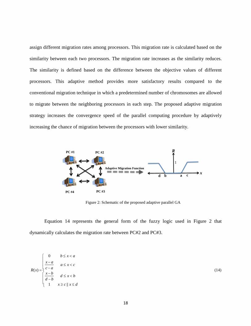
Figure 2: Schematic of the proposed adaptive parallel GA ......................................................... 18
Figure 3: 119-bus distribution network with aged and risky switches shown in red and thicker
lines [49] ........................................................................................................................... 24
Figure 4 : The hourly load data of the studied year ...................................................................... 25
Figure 5: The computed LCRI for each class ............................................................................... 25
Figure 6: (a) Total fitness; (b) Number of Switching ................................................................... 26
Figure 7: The optimal network configuration for class #19 ......................................................... 27
Figure 8: Power loss values corresponding to class #19............................................................... 28
Figure 9: The operation of initial tie switches .............................................................................. 28
Figure 10: Pareto frontier identified by a typical Pareto-dominance algorithm ........................... 34
Figure 11: A radial network with two loops ................................................................................. 37
Figure 12: The fuzzy functions calculating SRI for each switch .................................................. 39
Figure 13: The sample network used to clarify the adaptive local search step............................. 44
Figure 14: A 136-bus distribution network with 21 loops (Loop #16 contains branch numbers {1-
7, 136, 73, 70, 63-68, 99-101, 103-107, 110, 153, 45-47, 43, 42, 40, 39}) [57] .............. 47
Figure 15: The determined SRI of each switch ............................................................................ 49
Figure 16: The number of AS members ....................................................................................... 50
Figure 17: The declining trend of average fitness values ............................................................. 51
viii
Figure 18: The declining trend of fitness values ((a): average; (b): power loss; (c) voltage sag; (d)
THD) ................................................................................................................................. 53
Figure 19: The identified Pareto frontier .................................................................................... 53
Figure 20: The fuzzy function determining P1 ............................................................................. 59
Figure 21: The fuzzy function determining P2 ............................................................................. 60
Figure 22: The fuzzy function determining P3 ............................................................................. 61
Figure 23: Case study [62] ............................................................................................................ 62
Figure 24: The trend of the best fitness value in each generation ................................................ 65
Figure 25: The trend of the average and the best fitness value in each generation ...................... 66
Figure 26: The final solution......................................................................................................... 67
Figure 27: The power loss of each branch .................................................................................... 68
Figure 28: The trend of average fitness values ............................................................................. 69
Figure 29: The flowchart of algorithm.......................................................................................... 72
Figure 30: A radial network with three loops ............................................................................... 73
Figure 31: Updating the archive set members .............................................................................. 74
Figure 32: Determining the fitness fuzzy value for classification ................................................ 75
Figure 33: The case study [63]...................................................................................................... 77
Figure 34: The number of AS members found by the algorithm .................................................. 79
Figure 35: The declining trend of average voltage drop ............................................................... 80
Figure 36: The declining trend of average voltage sag ................................................................. 81
Figure 37: The frontiers identified by the algorithm for three scenarios ...................................... 82
Figure 38: The voltage profile of configurations presented in Table 2 ........................................ 83
Figure 39: The small case study for exhaustive search................................................................. 87
ix

Figure 40: The configuration with minimum power loss ............................................................. 89
Figure 41: The configurations with (a): minimum voltage sag and (b): minimum THD ............. 90
x
LIST OF TABLES
Table 1: Description of Added DG Units to the Network (Power Factor= 0.8 lag) ..................... 23
Table 2: Performance of Different Scenarios ............................................................................... 29
Table 3: Nonlinear Load Data (Percentage of Fundamental Frequency) ..................................... 48
Table 4: Performance of Different Algorithms ............................................................................. 52
Table 5: The Effect of the Proposed Reliability-based Encoding Strategy on the Performance of
the Algorithm .................................................................................................................... 55
Table 6: The Description of Different Scenarios .......................................................................... 78
Table 7: The Configurations with the Lowest Voltage Drop ....................................................... 82
Table 8: The Configurations Located at the Center of Pareto Frontiers ....................................... 84
Table 9: The Suboptimal Configurations Identified for Scenario #3 ........................................... 85
Table 10: Branch Data of the Small Case Study ........................................................................... 88
Table 11: Bus Data of the Small Case Study ................................................................................ 88
Table 12: Nonlinear Load Data of the Small Case Study (Percentage of Fundamental Frequency)
........................................................................................................................................... 88
xi
CHAPTER ONE: INTRODUCTION
Ever growing deployment of distribution automation (DA) technologies in distribution
systems has made the skeleton of the power grids more flexible. The network topology can be
dynamically reconfigured to optimally utilize the power grids. Distribution network
reconfiguration is a common problem in distribution management systems which is proposed by
Merlin and Back in 1975 [1]. Distribution network reconfiguration is the act of opening and
closing the switching devices of power systems to reach a topology that optimizes the desired
objectives.
Distribution systems reconfiguration has a variety of applications such as power loss
reduction [2], load balancing [3], improving power quality [4], increasing distributed generation
(DG) penetration [5], decreasing the number of switching operations [6], enhancing voltage
stability margin [7], and system restoration [8].
The distribution automation usually aims at optimizing more than one objective function.
There are mainly two techniques to solve multi-objective optimization problems: (1) Assigning
different significance factors to the objective functions, adding them up and solving the
optimization problem to optimize the resulted single function; (2) Adopting a Pareto dominance-
based algorithm to provide a set of optimums instead of only a single solution. The advantage of
the second option is that it provides alternative solutions. Therefore, the operator has more
flexibility to select the best possible solution from the identified Pareto frontier based on the
condition of the network.
1

The main challenge of implementing distribution network reconfiguration problem is the
high number of different possible switching combinations in a network to be considered and
analyzed as the candidates of the optimal configuration. That is why network reconfiguration is
known as a combinatorial, non-linear, non-differentiable constrained optimization problem.
Therefore, researchers have shown interest to employ meta-heuristic intelligent global
optimization algorithms in order to solve this NP-hard problem. Examples of these evolutionary
algorithms are genetic algorithm (GA) [9-10], partial swarm optimization (PSO) [11], harmony
search algorithm (HSA) [12], honey bee mating optimization (HBMO) [13], tabu search
algorithm (TSA) [14], ant colony optimization (ACO) [15], simulated annealing immune (SAI)
[16], and artificial neural network (ANN) based algorithms [17-18].
This dissertation contains seven chapters. In the second chapter, an adaptive parallel GA
is proposed to solve the problem of network reconfiguration when the time varying nature of
electric load is taken into account. A Pareto based SFLA is proposed in the third chapter to
resolve the main shortcoming of the presented method in Chapter 2. The proposed GA in
Chapter 2 is improved in Chapter 4 to be able to automatically modify its parameters during the
optimization process in order to enhance its efficiency in identifying more fertilized solutions.
The proposed method in Chapter 3 is modified in Chapter 5 and the problem of network
reconfiguration is solved in a smart grid in the presence of distributed generations (DGs). This
chapter elaborates how the quality of suboptimal solutions will be affected when DG units are
continuously added to the distribution network. The efficiency of the proposed method in
Chapter 3, which is modified in Chapter 5, is verified by comparing the simulation results with
an exhaustive search. Finally, Chapter 7 concludes this dissertation. The description of the
2

optimization methods proposed in this dissertation to solve the network reconfiguration problem
for the aforementioned concerns are briefly described in the rest of this chapter.
1.1 Adaptive parallel GA
The distribution network reconfiguration, depending on how the load is modeled, can be
dynamic or static. In static optimal distribution network reconfiguration, the loads are assumed to
be one single constant value in entire optimization process. Although this assumption
significantly reduces the computational burden of the algorithm, it cannot realistically model and
cover the impacts of load variations. Therefore, the time varying nature of the loads needs to be
taken into account [19-21]. For instance, in [22] to consider the impact of load variations a
dynamic network reconfiguration method is proposed in which the optimization procedure is
executed repetitively every hour as the load value varies.
Solving the optimization problem over a long period of time is computationally
expensive; especially in large-scale distribution systems with a large number of switches and so
many load condition scenarios. In order to address this issue, an intelligent and computationally
efficient algorithm is proposed in the second chapter. Fuzzy C-Mean (FCM) is utilized to cluster
the loading patterns into few clusters. This process significantly reduces the computational
burden of the long run optimization procedure.
To efficiently encode the radial network topology, a method based on Dandelion
encoding algorithm is developed. The proposed method assures that all the generated
3

chromosomes in the reconfiguration process automatically construct feasible radial
configurations. This significantly improves the convergence speed of the algorithm as the tedious
task of checking the radiality of the generated population is not needed any more.
In order to solve the optimization problem, a novel adaptive fuzzy-based parallel GA is
proposed in which the migration rates among different processors are dynamically modified
according to fuzzy rules. The proposed method reduces the computation burden of
reconfiguration problem through parallel computing. Also, by developing an adaptive migration
strategy based on fuzzy logic, it prevents the optimization algorithm from converging into local
optimums.
The objective functions defined for the proposed method are power loss, number of
switching and voltage drop. The strategy of assigning different significance factors is adopted to
introduce one single objective function to the algorithm. The performance of the proposed
reconfiguration method is demonstrated on a 119-bus distribution network.
1.2 Fuzzy Pareto dominance shuffled frog leaping algorithm
In the third chapter, a novel hybrid optimization model, which is a combination of fuzzy
Pareto dominance (FPD) technique and shuffled frog leaping algorithm (SFLA), is proposed to
identify a Pareto frontier as a set of high-quality suboptimal configurations for the network.
SFLA is a meta-heuristic population based cooperative search method originated from natural
memetics [23]. It provides a frog leaping rule for local search and a memetic shuffling rule for
4

global information exchange [24]. This global optimization algorithm is much faster in
convergence compared to the other prominent evolutionary algorithms [25].
To consider the reliability of switching procedure, a reliability based frog coding is
proposed in which a Switch Reliability Index (SRI) is defined for each switch. SRI is a fuzzy
value between zero and one. A switch with a higher value of SRI has the higher chance to be
selected for generating the initial population of the optimization process. Using the proposed
reliability based frog coding, aged switches or the switches located at critical points of the
network will be less participated in the process of network reconfiguration. Moreover, a
systematic approach is proposed to adapt the local search step of SFLA for the application of
distribution network reconfiguration so that only feasible frogs (i.e. radial configurations) are
automatically born. This idea significantly increases the convergence speed of the conventional
SFLA.
The objective functions to be optimized by the proposed algorithm are power loss,
voltage sag and total harmonic distortion (THD) as two main indices of power quality. The
strategy of Pareto dominance is utilized to recognize the suboptimal solutions identified by the
optimization algorithm. The efficiency of the proposed method is verified on a large scale 136-
bus electricity distribution network.
1.3 Dynamic fuzzy genetic algorithm
One of the most highly used methods in order to solve the network reconfiguration
5

optimization problem is genetic algorithm (GA). GA is a multi-dimensional and stochastic
search strategy performing based on the idea of natural selection of chromosomes during the
process of evolution. The main concentration of this algorithm is to set a reasonable trade-off
between exploitation and exploration. If it focuses more on exploitation, the probability of
getting stuck in a local optimum increases. On the other hand, higher exploration slows down the
convergence process.
Therefore, there should be a meaningful interaction between the GA parameters (i.e.
crossover probability and mutation probability) in order to boost the efficiency of GA
performance [26]. For the purpose of identifying the optimal network configuration, GA is
utilized in [27] in which the parameters are considered to be fixed values. In order to set a better
balance between exploitation and exploration and avoid poor parameterization, researchers have
proposed different techniques to determine the GA parameters dynamically as the algorithm
proceeds and adjust them so that GA does not fall into local optimums while its convergence
speed does not slow down. A "messy" approach is proposed in [28] to calculate and update the
crossover and mutation probabilities based on the proportion of individual's fitness value and
average fitness value compared to the best fitness value. A two-level adaptive system is proposed
in [29] to dynamically determine and update the GA parameters "population size", "crossover
rate", "mutation rate", "generation gap", "scaling window" and "selection strategy". The GA
parameters are adopted in [30] based on the environmental constraint of maximum population
size. In this technique, GA operators are considered as alternative reproduction strategies and
fighting among individuals is permitted. A fuzzy logic controller (FLC) is proposed in [31] to
adaptively tune the crossover rate based on the individuals' age in order to preclude the
6

premature convergence and improve the emulation of the biological process.
In the fourth chapter, the optimization problem of electric distribution reconfiguration is
solved by a GA that employs three fuzzy functions to adaptively tune its crossover and mutation
rates. The first fuzzy rule is defined based on the position of each chromosome compared to the
best chromosome in the same generation. The second fuzzy rule is introduced on the basis of the
situation of all the chromosomes compared to the best chromosome in the same generation. The
output of the third fuzzy rule depends on the lifetime of each chromosome. Defining these three
fuzzy functions, the probability of crossover and mutation changes as the algorithm proceeds and
the premature convergence is avoided while the convergence speed of identifying the global
optimal configuration does not decrease.
1.4 Adaptive fuzzy shuffled frog leaping algorithm
The concentration of the fifth chapter is to analyze a potential smart grid solution to more
high-quality suboptimal configurations of distribution networks. This new paradigm of electrical
grids proposes the adoption of two-way flows of electricity and builds a distributed energy
delivery network. As a result, utilities are enforced to evolve their classical topologies to
accommodate distributed generation (DG). DG units are categorized in two main groups: (1)
conventional generation resources such as gas turbines, diesel generators, fuel cells, and battery
banks; (2) renewable energy resources such as wind turbines, solar cells, hydro power, and
hybrid wind-PV-battery system. The idea of decentralized generation suggests the generation of
7

electricity from many small energy resources with the purpose of improving the security of
supply and decreasing the environmental impacts of excessive burned fossil fuels in central
plants.
Considering the noticeable growing trend of on-site generation units in distribution
systems over the last years, researchers have shown interest to solve the problem of network
reconfiguration in the presence of DGs. In [32] a particle swarm optimization (PSO) algorithm is
presented to solve network reconfiguration problem with the purpose of maximizing DG
integration and minimizing total power loss. A meta-heuristic harmony search algorithm (HSA)
is employed in [33] to simultaneously solve the optimal DG placement and network
reconfiguration problems to optimize power loss and voltage profile. Optimal locations of DG
units are recognized by sensitivity analysis in this study. A genetic algorithm is utilized in [5] to
reconfigure distribution systems so that it maximizes the penetration of DG units while it
optimizes voltage profile and thermal constraints (i.e. total loading of the branches). In [34]
operation strategies are taken into account to utilize network reconfiguration of automated
distribution systems in the presence of DGs as a real-time operation to optimize power loss and
service restoration. An artificial bee colony (ABC) algorithm is presented in [35] to optimally
reconfigure a distribution network containing hybrid renewable systems (wind turbines & solar
cells) as DGs so that the total power loss, the total electrical energy cost, and the total reduced
emission of atmospheric pollutants are optimized.
A Pareto-based global optimization algorithm is proposed in the fifth chapter to solve the
multi-objective problem of distribution system reconfiguration with the purpose of optimizing
8

voltage profile and voltage sag. The optimization method utilizes a Pareto dominance technique
to recognize non-dominated solutions identified by SFLA which is adapted in the encoding and
partitioning steps. Developing this Pareto-based optimization technique, the system operator will
not have to rely on only one single solution. The algorithm will identify a set of high-quality
suboptimal solutions on the Pareto frontier which are unable to dominate each other. Any of the
recognized solutions on the Pareto frontier might be adopted as a candidate network
configuration based on the situation of system. A fuzzy logic is introduced in the partitioning
step of SFLA based on the values of voltage drop and voltage sag in order to provide a more
accurate criterion for the classification of frogs.
9

CHAPTER TWO : OPTIMAL DYNAMIC RECONFIGURATION OF
LARGE-SCALE DISTRIBUTION SYSTEMS WITH TIME VARYING
LOADS USING PARALLEL COMPUTING
2.1 Problem formulation
In this chapter the following objectives are selected for optimal network reconfiguration:
(1) power losses; (2) voltage deviation from the nominal value; and (3) the number of switching.
1 1 1 2 2 2 3 31 1 1 1 1
( * ( . ) * ( . ) * ( . . ))365 365
C C K C Ci i ki i
ij k iji i k j i
D DMax k fit F k fit F k fit N w x
= = = = =
+ +∑ ∑ ∑∑∑ (1)
1 1
1Nf m
lf
f l
F Ploss= =
=∑∑ (2)
2
22 )()(lf
lf
lfl
flf
V
QPrPloss
+=
(3)
∑=
−=N
nnVVF
1
max2 (4)
Subject to
min maxnV V V≤ ≤ (5)
maxl lI I≤ (6)
snNm −= (7)
.A I L= (8)
10

where, the dynamics are i, j and k. i and j count the number of clusters (classes). And k refers to
the switch number. C represents the total number of clusters. The concept based on which
clusters are defined will be explained in Section 2.4. lfPloss denotes the line loss of branch l in
feeder f. lfP , l
fQ , lfV and l
fr stand for the active power, reactive power, voltage and the resistance
value of the head node of feeder f and branch l, respectively. nV , lI and maxlI represent the
voltage of bus n, the current of branch l and the maximum allowed value of lI , respectively. iF1
and iF2 , respectively, refer to F1 and F2 for the loading condition at class i. Di is the number of
days that are assigned to cluster i. Nij signifies the total number of transitions from class i to class
j in the year under study. kijx is a binary variable with the default value of zero. If in the transition
from class i to j the status of switch k is changed, the value of kijx becomes one. That is why this
variable represents the connectivity of the relevant switch (branch).
A weighting factor of w is assigned to each switch based on how much a given switch is
desired to participate in the process of network reconfiguration. For instance, the assigned value
of w to a given switch could be increased according to asset management monitoring data as the
switch ages. Therefore, the possibility of participation of that switch in the reconfiguration
process reduces. Another scenario could be a case when a given switch is located at a critical
location of the network and changing its status is not desirable as it may cause disturbances that
are not tolerable by adjacent sensitive loads or it might lead to loss of a significant portion of the
network. In these cases also a higher value can be assigned to w associated to the switch.
K stands for the total number of switches. m, Nf, N and ns are the total number of
branches, feeders, nodes (buses) and energy sources, respectively. I is the m-vector complex
11

branch current, L is the n-vector complex nodal current, and A is the n×m node-to-branch
incidence matrix. k1, k2 and k3 are weighting factors for power loss, voltage deviation and
number of switching which are defined by the operator based on the relative importance of the
corresponding objective. For instance, if the main concentration of the operator is on the
minimization of power loss, a higher value is assigned to k1 (e.g. k1=0.7, k2=0.2, k3= 0.1). fit1, fit2
and fit3 are the relevant fuzzy membership functions defined by operator to scale and restrain the
variables between zero and one. These functions should be defined so that maximizing the output
of these functions is equivalent to minimizing their corresponding arguments (i.e. power loss,
voltage deviation or switching number). For example, if 11. 0
365C iii
DF
==∑ then, 1 11
( . )365
C iii
Dfit F
=∑
should be equal to one.
2.2 Chromosome encoding
Efficient distribution network topology encoding significantly reduces the computational
burden of the optimization procedure. The most straightforward but the least efficient encoding
method is constructing a string formed by the binary status of the switches (closed/open) [10].
This technique requires an extra function to be integrated into the GA structure to check the
radiality of network topology. A distribution network is called radial when there is only one path
between each node (bus) and the source (Node #1). A vertex encoding method based on the
Prufer number is presented in [36] in order to avoid the tedious radiality check procedure of GA.
This strategy relies on the number of nodes (i.e. buses) in the network instead of the number of
12

switches or branches. An edge-set encoding based algorithm is proposed in [37]. The bits of each
chromosome, generated by this method, refer to the branch numbers that are connected together
directly or indirectly. A Matroid theory based GA encoding algorithm is proposed in [10] in
order to solve the network reconfiguration problem faster without checking the distribution
network radiality. In [38] an analytic comparison of six classical tree graph encoding techniques
(i.e. characteristic vector, Prufer numbers, network random keys, edge sets, node biased
encoding, and link and node biased encoding) are provided. The performance of GA using each
of these encoding strategies has been analyzed as well. Two sequential encoding techniques
called subtractive and additive are proposed in [9] to generate radial topologies for solving
network reconfiguration problem. An encoding method based on the Prufer number and a
clustering string is presented in [39] for solving optimal spanning tree problem in
communication systems.
The power distribution systems encoding/decoding method not only should generate
radial configuration but also needs to prevent “infeasible radial network” that refers to the
generated topologies in which the buses with no switch in between are connected together.
Moreover, the implementation of the coding strategy should not be too complicated.
Dandelion coding method is proposed in [40] to encode spanning trees in communication
systems. Dandelion strategy is one of the most computationally efficient encoding techniques
for spanning trees. This coding scheme exhibits a noticeably higher locality and heritability
compared to the other encoding strategies like Blob code, Prufer code and direct tree code [40].
Furthermore, if the problem size increases, its locality improves as well. These features make
this method very appropriate for large-scale networks.
13

In this chapter the problem of finding the optimal radial topology is formulated as
identifying the optimal feasible spanning tree. It should be mentioned that “tree” and “radial
network” refer to the same concept in this dissertation. A network encoding algorithm based on
Dandelion theory is developed for the application of electrical distribution networks that
generates "Radial & Feasible" structures. The procedure for implementing the encoding strategy
is as follows:
0) Set k=0;
1) Randomly generate vector S1 containing n-2 components whose elements are
selected from the set {1,2,...,n} where n refers to the number of nodes;
2) Develop matrix S2 whose second row is S1, and the first row is the vector [2,
3,...,n-1];
3) Switch the first and second row of S2 and call the generated matrix S3. Then,
build vector S4 whose components are the common columns in S2 and S3;
4) Sort the components of S4 in a descending order, delete the repetitive components
and call the generated vector S5;
5) In order to keep the radial topology of the distribution network with multiple
feeders, connect all the root nodes (substations) to each other with a “virtual line”.
6) Connect the nodes of S5 to each other. Then, connect node 1 to the first
component of S5, and node n to the last element of S5. Finally, connect the elements in the
first row of S2 to the corresponding components existing in the second row of S2.
7) The generated chromosome using this node-based coding is always radial.
However, after constructing the radial chromosome its feasibility should be checked in this
14

step. If the generated chromosome is feasible, set k=k+1. It is notable this branch checking
process takes considerably less time in comparison to the checking of radiality of the
chromosomes in conventional binary coding.
8) If the generated tree in the previous step is feasible, remove the virtual line and
the developed chromosome will be still radial.
9) If k is equal to the desired number of population, go to 10; otherwise go to 1.
10) Finish.
The following example explains the encoding method numerically. Consider a network
with n=9 nodes:
Step 1)
[ ]1 5 6 8 2 6 4 9S = (9)
Step 2)
2 3 4 5 6 7 82
5 6 8 2 6 4 9S
=
(10)
Step 3)
5 6 8 2 6 4 93
2 3 4 5 6 7 8S
=
(11)
{ }4 (2,5), (5, 2), (6,6)S = (12)
Step4)
15

{ }5 2,5,6S = (13)
Step 5) It is assumed there is only one substation in the network. Therefore, there is no
need to consider the virtual links.
Step 6) Figure 1 (a) depicts the corresponding tree to chromosome S1. As it can be
realized from the figure, a unique tree can be assigned to any other chromosome using this
encoding technique.
Step 7) According to Figure 1 (a), the generated tree for S1 is feasible. In this example, it
is assumed that only the adjacent nodes can be connected together.
Now if the same procedure is repeated for the initial random vector S1'= {9, 3, 1, 7, 8, 5,
3}, one can attain the relevant tree illustrated in Figure 1 (b). In this radial network, the
connections between 1-7, 3-9, 9-2, and 8-3 are not possible which makes this tree an infeasible
distribution network. Therefore, in Step 7 the created vector is removed from the initial
population of the optimization procedure.
(a)
(b)
Figure 1: (a) The corresponding tree for chromosome S1; (b) The corresponding tree for chromosome S1’
1 2
7
5
8
4 6
9
3 1 2
7
5
8
4 6
9
3
16
2.3 Adaptive parallel GA
Parallel Genetic algorithms (PGAs) are considered as a class of guided random
evolutionary algorithms [41]. While PGAs still have the benefits of serial GAs (i.e. robustness,
easy customization for new problems, and multiple solution capabilities), they also have higher
efficiency (i.e. super numerical performance) [42], larger diversity maintenance [43], additional
availability of CPU [44], and higher speed in comparison to serial GAs. The PGAs can be
categorized into three general groups: (1) Master-slave PGA; (2) Fine-grained PGA; (3) Multi-
deme PGA. In a master-slave PGA, there is only one united population in which the evaluations
of chromosomes are distributed by scheduling fractions of population among different
processing slave units. A fine-grained PGA contains only one spatially structured population.
Selection and mating in this method are limited to small groups to avoid groups' overlapping and
disseminating better individuals across the entire population. A multi-deme PGA contains
several populations that exchange their chromosomes occasionally based on a process called
migration. More details about these three PGA approaches can be found in [45].
One important factor that has a direct impact on the performance of multi-deme PGA is
the utilized migration strategy. In conventional methods the migration rate is a predefined fixed
value. However, as optimization is a dynamic process, developing adaptive migration rate that is
dynamically calculated and updated based on the current status of different demes, will improve
the algorithm in terms of speed and quality of final result.
Figure 2 depicts the proposed adaptive parallel GA. After each certain number of
generations, an adaptive migration strategy based on a fuzzy logic is applied to dynamically
17
assign different migration rates among processors. This migration rate is calculated based on the
similarity between each two processors. The migration rate increases as the similarity reduces.
The similarity is defined based on the difference between the objective values of different
processors. This adaptive method provides more satisfactory results compared to the
conventional migration technique in which a predetermined number of chromosomes are allowed
to migrate between the neighboring processors in each step. The proposed adaptive migration
strategy increases the convergence speed of the parallel computing procedure by adaptively
increasing the chance of migration between the processors with lower similarity.
Figure 2: Schematic of the proposed adaptive parallel GA
Equation 14 represents the general form of the fuzzy logic used in Figure 2 that
dynamically calculates the migration rate between PC#2 and PC#3.
0
( )
1 ||
b x ax a a x cc aR xx b d x bd b
x c x d
≤ < − ≤ < −= − ≤ < − ≥ ≤
(14)
PC #1
PC #4 PC #3
PC #2
Adaptive Migration Function
a cbd
1
x
R
18

where, x stands for the absolute difference value between the average fitness values of PC #2 and
PC #3. A higher difference value causes a more crowded population of migrating chromosomes
between the corresponding PCs. In Equation 14 a higher difference value of a-c or b-d increases
the diversity in the migration procedure. Therefore, it is a trade-off between not falling into local
optimums and the spread of convergence.
At a later stage, the computed migration rate (R) is multiplied by the maximum allowed
number of transferring chromosomes to attain the number of individuals to be exchanged
between these two PCs. The same procedure is carried out for every two other PCs.
After determining the number of migrating chromosomes, a systematic strategy should be
employed to select the chromosomes which need to be migrated. Randomly selecting the
chromosomes may prevent selecting the most fertilized individuals for the migration. On the
other hand, selecting the chromosomes with highest objective values may lead to immature
convergence and trapping the algorithm in local minima. To address this issue, the roulette-
wheel selection technique [46] is utilized in the proposed migration strategy. In this method, the
chromosomes with higher objective values have a higher chance to be selected for the migration
process. However, there is still a chance for the less fertilized individuals to be migrated with the
hope of transferring the new and rare features (genes) to the other PCs.
2.4 Reducing load condition scenarios using fuzzy C-mean classifier
In the proposed optimal distribution network reconfiguration method, the time varying
19
nature of the loads is taken into account. However, performing the optimization algorithm for
every possible load condition scenario is not computationally practical. To address this issue, the
load scenarios are reduced by clustering the daily load data. Fuzzy C-Mean (FCM) algorithm
[47] is utilized for this classification purpose. One of the most significant advantages of this
clustering technique is that it provides more accurate results for overlapped nontrivial samples
compared to other clustering techniques such as k-means algorithm [48].
In this method, the desired number of classes as well as initial clustering seeds is
determined in the first stage. This algorithm updates the location of seeds (daily load curves) in
each iteration and then a fuzzy membership vector, containing the degrees of membership to
each of the clusters, is assigned to each seed. The membership degrees are assigned based on the
distance between each seed and the centers of other clusters. The highest membership degree
(i.e. the least distance value) in each fuzzy vector indicates the corresponding class of the
relevant daily load curve. The required procedure to implement FCM method is detailed in [47].
In the proposed optimal reconfiguration algorithm, once the daily load data over the
studied year are classified using FCM classifier, Load Class Representative Index (LCRI) is
defined as the average value of each class which is used as the representative of each class in the
process of the optimization.
Using the employed load scenario reduction method, the 365 daily load data are reduced
to only M LCRI values which significantly reduces the computational burden of the
optimization process.
20

2.5 Implementation
The following pseudo code represents the implementation procedure of the proposed
algorithm.
1) Apply FCM classifier algorithm to the existing 365 daily load curves of the
studied year.
2) Put Day_counter=1.
3) If the optimal configuration of Class (Day_counter) has been already
determined, put Day_counter= Day_counter +1 and go to step 2; otherwise, go to step 4.
4) Calculate the corresponding LCRI (Class(Day_counter)), and consider that
value as the electricity demand of the network.
5) Create N radial and feasible structures, through implementing the ten steps
elaborated in section 2.2, as the initial population of GA.
6) Locate the N chromosomes in different PCs equally. Implement the following
steps for all the PCs in parallel.
7) Put Generation=1.
8) Run the power flow algorithm and calculate the fitness value for each
chromosome using Equations 1-4 provided in section 2.1.
9) Apply the adopted selection operator to determine the individuals participating
in the mating pool.
10) Apply the selected crossover and mutation strategies to specify the chromosomes
taking part in the next generation.
21

11) If [Generation/Migration_gap] equals an integer value, apply the proposed
adaptive fuzzy based migration strategy to determine the number of chromosomes to be
transferred between each two parallel processors. Otherwise, go to step 13.
12) Apply the roulette-wheel selection technique to select the individuals to be
transferred mutually between each two processors.
13) If Max_Generation=Generation, go to step 14. Otherwise, Generation=
Generation+1 and go to step 8.
14) Print the identified individual with the highest fitness value in all the PCs as the
best configuration of the corresponding class.
15) If Day_counter=365, go to step 16. Otherwise, Day_counter= Day_counter+1
and go to step 3.
16) Finish.
2.6 Simulation results and discussions
The proposed algorithm is implemented in MATLAB software on a computer with the
processor of Intel(R) Xeon(R) CPU E5-2603 0 @ 1.80 GHz. The network shown in Figure 3 is
selected as a platform for implementing the algorithm. It is a 119-bus distribution network
presented in [49] with a difference that five distributed generation (DG) units are added to the
system. The tie switches are numbered and presented with dash lines. Table 1 presents the
location and the capacity of the added DG units.
22

As it was mentioned in 2.1, a weighted sum of three different fitness values is optimized
in this chapter. In this study, K1, K2, and K3 are assumed to be equal (i.e. 0.333), which means all
the three fitness values have the same importance in the optimizing process.
Table 1: Description of Added DG Units to the Network (Power Factor= 0.8 lag)
DG1 DG2 DG3 DG4 DG5
Bus No.
27 56 65 94 118
Output (MW)
0.1 0.15 0.3 0.2 0.2
In Figure 3, the aged switches or the switches that are located at sensitive locations are
presented with red and thicker lines. As it was discussed in section 2.2, these switches are
desired not to participate in the reconfiguration process. To reach this goal, the operator can
simply assign a higher value of w in Equation 1 for the aged or more critical switches.
23

Figure 3: 119-bus distribution network with aged and risky switches shown in red and thicker lines [49]
The assumed hourly load of the studied network over a year is depicted in Figure 4. For
this application, FCM is implemented to classify the daily load curves into 20 (M=20) classes.
The computed LCRI together with the number of days belonging to each class are presented in
Figure 5. For example, the class no. 4 has the highest value of LCRI (7023.9 MW). This class
represents 16 days of the year. Once the optimization problem is solved, a certain optimal
configuration is found for each day of the year. For example, the class no. 19 contains 15 daily
load curves related to days #186, 190-191, 196-197, 199-201, 204-207, and 211-213. It means
that the configuration identified by the optimization algorithm for class #19 is utilized for the
119
120
121
122
123
105
106
107
108
109
110
111
112
113
114
115
117
118116
66
67
68
69
70
71
72
73
74
75
76
77
78
79
80
DG5
89
90
91
81
82
83
84
85
86
87
88
93
94
95
96
97
98
99
100
101
102
103
2
4
5
6
7
3
8
9
29
30
31
32
33
34
35
36
49
50
51
52
53
54
55
56
3738
58
59
6061
62
63
64
65
DG4
DG3
DG2
40
41
42
43
44
45
46
47
48
10
11
18
19
20
21
22
23
24
25
26
27
DG1
S1
2
3
4
5
6
7
8
910
12
13
11
14
15
1
24
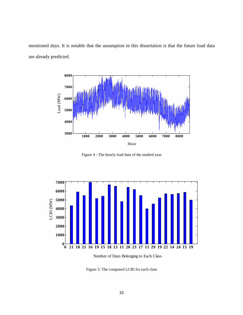
mentioned days. It is notable that the assumption in this dissertation is that the future load data
are already predicted.
Figure 4 : The hourly load data of the studied year
Figure 5: The computed LCRI for each class
1000 2000 3000 4000 5000 6000 7000 80003000
4000
5000
6000
7000
8000
Hour
Load
(MW
)
0 21 18 21 16 19 15 18 13 11 20 23 17 11 29 19 22 14 24 15 190
1000
2000
3000
4000
5000
6000
7000
Number of Days Belonging to Each Class
LCR
I (M
W)
25

The proposed parallel GA model is implemented on four processors each of which
containing 100 chromosomes. It is assumed that after each 10 iterations (i.e. migration gap), the
adaptive fuzzy migration strategy, discussed in section 2.3, is carried out among all the
processors. Figure 6 illustrates the increasing trend of the total fitness value as well as the
declining trend of number of switching for the four parallel PCs during 30 generations.
According to Figure 6, PC #3 identifies the most fertilized solution because of its efficient
migrations at iteration #10 and #20.
Figure 6: (a) Total fitness; (b) Number of Switching
The configuration identified by the optimization algorithm for class #19 is presented in
Figure 7. The operator should apply this configuration at the days corresponding to class #19.
The open switches for this configuration are shown by red and bold dash lines. It is notable that,
the status of the aged and risky switches has not been changed as it was desired.
0 10 20 30
0.45
0.5
0.55
0.6
0.65
0.7
0.75
(a)
0 10 20 301800
1900
2000
2100
2200
2300
2400
2500
2600
2700
2800
(b)
PC #1PC #2PC #3PC #4
PC #1PC #2PC #3PC #4
26

Figure 7: The optimal network configuration for class #19
Figure 8 illustrates how the power loss of each branch changes after optimal
reconfiguration of the network for class# 19. According to Figure 8, the branch power loss
values significantly reduce in the identified network configuration.
119
120
121
122
123
105
106
107
108
109
110
111
112
113
114
115
117
118116
66
67
68
69
70
71
72
73
74
75
76
77
78
79
80
DG5
89
90
91
81
82
83
84
85
86
87
88
93
94
95
96
97
98
99
100
101
102
103
2
4
5
6
7
3
8
9
29
30
31
32
33
34
35
36
49
50
51
52
53
54
55
56
3738
58
59
6061
62
63
64
65
DG4
DG3
DG2
40
41
42
43
4445
46
47
48
10
11
18
19
20
21
22
23
24
25
26
27
DG1
S1
2
3
4
5
6
7
8
910
12
13
11
14
15
1
12
13
14
15
16
17
27

Figure 8: Power loss values corresponding to class #19
The schedule of all the initial tie switches over the studied year is illustrated in Figure 9.
The vertical axis presents the number of classes in which the corresponding tie switch will be
closed. According to this figure, the status of tie switches #9 and #1 do not change at all (stay
open) and the status of switch #3, 4 and 13 stay the same (closed) in most classes.
Figure 9: The operation of initial tie switches
Finally, the performance of the proposed algorithm is compared with that of GA with
only one PC (i.e. parallelism is not used) and conventional parallel GA without the fuzzy
migration (i.e. migration rate is a fixed predefined number), as is shown in Table 2. This table
0 20 40 60 80 100 120 1370
0.2
0.4
0.6
0.8
1
Branch No.
Scal
ed P
ower
Los
s
PrimaryFinal
1 2 3 4 5 6 7 8 9 10 11 12 13 14 150
5
10
15
20
The Tie Switch Number
The
Num
ber
of C
lass
es
28
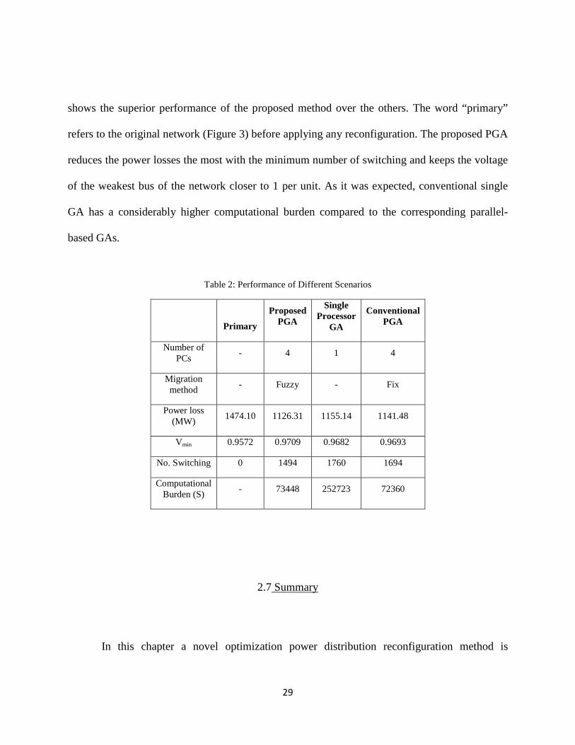
shows the superior performance of the proposed method over the others. The word “primary”
refers to the original network (Figure 3) before applying any reconfiguration. The proposed PGA
reduces the power losses the most with the minimum number of switching and keeps the voltage
of the weakest bus of the network closer to 1 per unit. As it was expected, conventional single
GA has a considerably higher computational burden compared to the corresponding parallel-
based GAs.
Table 2: Performance of Different Scenarios
Primary
Proposed PGA
Single Processor
GA
Conventional PGA
Number of PCs - 4 1 4
Migration method - Fuzzy - Fix
Power loss (MW) 1474.10 1126.31 1155.14 1141.48
Vmin 0.9572 0.9709 0.9682 0.9693
No. Switching 0 1494 1760 1694
Computational Burden (S) - 73448 252723 72360
2.7 Summary
In this chapter a novel optimization power distribution reconfiguration method is
29

proposed that identifies the high-quality suboptimal feasible topologies for large-scale networks
with time varying loads. The proposed method can tackle the computational burden of large-
scale power distribution systems reconfiguration by using parallel processing, efficient topology
encoding, and load scenario reduction. Fuzzy based migration strategy is proposed to
dynamically compute the number of fertilized chromosomes that should be migrated among the
processors of parallel GA. A modified Dandelion encoding is developed that reduces the
computational burden of classic binary coding strategy by automatically generating feasible and
radial topologies during the optimization process. An FCM clustering method is adopted to
decrease the considerable amount of load scenarios during the year under study.
One of the main advantages of the proposed dynamic power distribution systems
reconfiguration method is that the optimization process is carried out over a long period of time
in contrast to the existing methods that the optimization is re-executed every short period of time.
Therefore, by using the proposed method the accumulated objective functions are optimized.
30
CHAPTER THREE: A HYBRID PARETO DOMINANCE BASED
OPTIMIZATION METHOD FOR OPTIMAL DISTRIBUTION NETWORK
RECONFIGURATION
3.1 Problem formulation
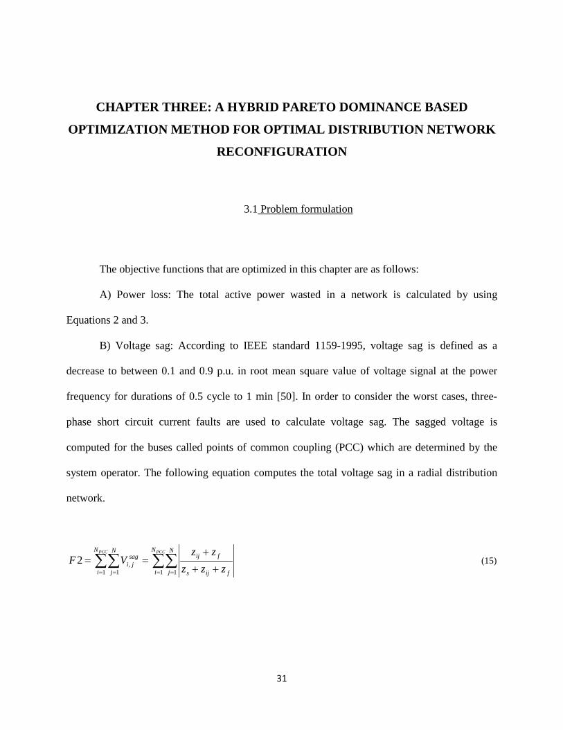
The objective functions that are optimized in this chapter are as follows:
A) Power loss: The total active power wasted in a network is calculated by using
Equations 2 and 3.
B) Voltage sag: According to IEEE standard 1159-1995, voltage sag is defined as a
decrease to between 0.1 and 0.9 p.u. in root mean square value of voltage signal at the power
frequency for durations of 0.5 cycle to 1 min [50]. In order to consider the worst cases, three-
phase short circuit current faults are used to calculate voltage sag. The sagged voltage is
computed for the buses called points of common coupling (PCC) which are determined by the
system operator. The following equation computes the total voltage sag in a radial distribution
network.
∑∑ ∑∑= = = = ++
+==
PCC PCCN
i
N
j
N
i
N
j fijs
fijsagji zzz
zzVF
1 1 1 1,2 (15)
31

where, sagjiV , signifies the voltage sag at bus i (a PCC) resulted from a fault at node j. zij refers to
the impedance between PCC and fault location j. zf and zs represent the fault impedance and the
source impedance at PCC. N and NPCC are the number of buses and the length of PCC,
respectively.
C) Total harmonic distortion (THD): THD is a criterion indicating the harmonic
distortion level in a system. As it is presented in Equation 16, THD is defined as the summation
of all harmonic components of a signal over the fundamental component [51].
∑∑
=
==pccN
i i
m
h
hi
V
VF
11
2
2
3 (16)
where, hiV is the voltage of bus i related to the harmonic h. And m denotes the number of
harmonics to be considered.
The following three constraints need to be satisfied:
min maxnV V V≤ ≤ (17)
maxl lI I≤ (18)
32
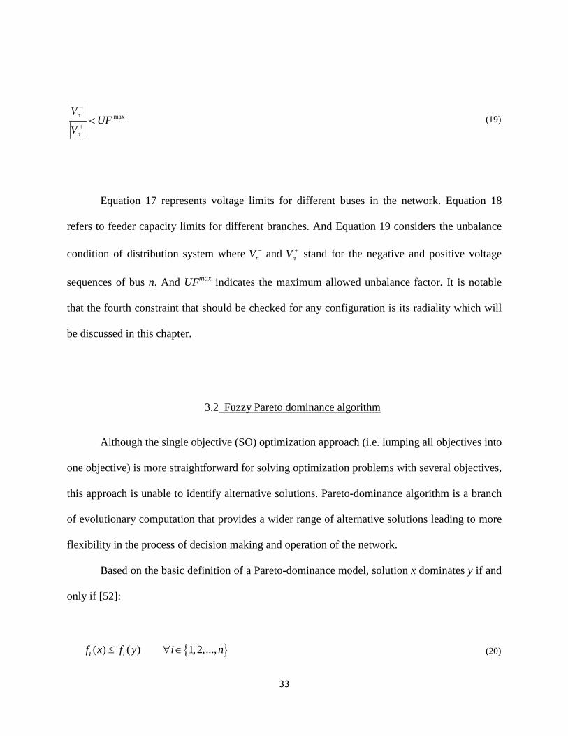
maxUFV
V
n
n <+
−
(19)
Equation 17 represents voltage limits for different buses in the network. Equation 18
refers to feeder capacity limits for different branches. And Equation 19 considers the unbalance
condition of distribution system where −nV and +
nV stand for the negative and positive voltage
sequences of bus n. And UFmax indicates the maximum allowed unbalance factor. It is notable
that the fourth constraint that should be checked for any configuration is its radiality which will
be discussed in this chapter.
3.2 Fuzzy Pareto dominance algorithm
Although the single objective (SO) optimization approach (i.e. lumping all objectives into
one objective) is more straightforward for solving optimization problems with several objectives,
this approach is unable to identify alternative solutions. Pareto-dominance algorithm is a branch
of evolutionary computation that provides a wider range of alternative solutions leading to more
flexibility in the process of decision making and operation of the network.
Based on the basic definition of a Pareto-dominance model, solution x dominates y if and
only if [52]:
{ }( ) ( ) 1, 2,...,i if x f y i n≤ ∀ ∈ (20)
33
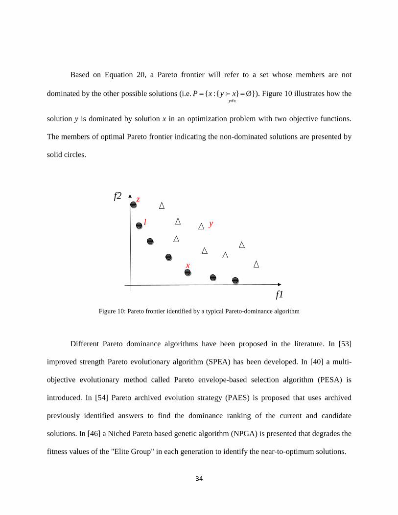
Based on Equation 20, a Pareto frontier will refer to a set whose members are not
dominated by the other possible solutions (i.e.xyxyxP
#}{:{ == Ø}). Figure 10 illustrates how the
solution y is dominated by solution x in an optimization problem with two objective functions.
The members of optimal Pareto frontier indicating the non-dominated solutions are presented by
solid circles.
Figure 10: Pareto frontier identified by a typical Pareto-dominance algorithm
Different Pareto dominance algorithms have been proposed in the literature. In [53]
improved strength Pareto evolutionary algorithm (SPEA) has been developed. In [40] a multi-
objective evolutionary method called Pareto envelope-based selection algorithm (PESA) is
introduced. In [54] Pareto archived evolution strategy (PAES) is proposed that uses archived
previously identified answers to find the dominance ranking of the current and candidate
solutions. In [46] a Niched Pareto based genetic algorithm (NPGA) is presented that degrades the
fitness values of the "Elite Group" in each generation to identify the near-to-optimum solutions.
f1
f2
x
y
z
l
34

In this chapter, fuzzy Pareto dominance (FPD) technique is utilized to recognize the non-
dominated network configurations identified by the global optimization algorithm. FPD assigns
certain levels of dominance between each two solutions based on mutual fuzzy-based dominance
degrees [53]. Therefore, FPD does not consider the solid circles in Figure 10 equally optimal.
This is the major advantage of this technique over the conventional Pareto-dominance models.
According to FPD, vector (i.e. solution) a is dominated by vector b at the degree of pµ
[53]:
min( , )( , )
i ii
pi
i
a ba b
bµ =
∏∏
(21)
where, a and b indicate fitness values of the corresponding solutions. The degree of dominance
varies between zero and one. If it equals to one, a is absolutely dominated by b. If ( , )p a bµ and
( , )p b aµ are both less than one, the vectors are non-dominated (e.g. the position of x and z in
Figure 10). Although y is not absolutely dominated by z, it cannot be considered as a member of
the optimal Pareto frontier since there is an l which has the same value of f2 but a lower value of
f1 compared to y.
Finally, the average of pµ is assumed as the rank of a:
}),({)(Mb
pM bameanar∈
= µ (22)
35

where, M represents all the possible answers.
The solution with the lowest value of (.)Mr stands for the most fertilized individual (i.e.
configuration).
3.3 A reliability based network encoding
One important step in optimal network reconfiguration is encoding the topology of the
network. In general, there are four major network (called “frog” in this chapter) coding
techniques: 1) Vertex (i.e. node) based methods [40] in which the number of bits of each frog
corresponds to the number of buses (i.e. nodes) in the network. This technique automatically
creates radial configurations but it leads to large-size frogs for large systems containing many
buses; 2) Branch based strategies [54] which automatically create radial frogs whose number of
bits is proportional to the number of branches in the network; 3) Binary switch based approach
which develops binary individuals (i.e. frogs) whose number of bits is the same as the number of
switches in the system. This technique does not guarantee producing radial configurations and
requires a tedious radial checking procedure to remove the infeasible frogs, 4) Loop (i.e. mesh)
based algorithms [55] that automatically create radial frogs. The number of bits in each frog is
equivalent to the number of meshes in the network.
As the number of loops in a system is noticeably less than the number of branches and
36

nodes, the loop-based strategy is computationally more efficient for encoding large distribution
networks. In this chapter, this approach is adopted to encode the SFLA frogs. Therefore, the
number of bits of each frog is equal to the number of loops in the network. Each bit indicates the
branch number, located in the corresponding loop that should be open. For instance, the encoded
frog for the network configuration shown in Figure 11 is F1= {10, 4}. As long as there is no
more than one open branch in each common feeder (in Figure 11 the common feeder refers to
branches #5 and #6), the developed frog represents a radial configuration. As an example, any
developed frog for the network presented in Figure 11 is radial except {6, 6}, {5, 5}, {6, 5} and
{5, 6}. It is notable that the infeasible configurations should be automatically avoided which will
be discussed in details in this chapter.
Figure 11: A radial network with two loops
It is desirable that the aged and risky switches less participate in the reconfiguration
procedure. To address this issue, in this chapter, a systematic approach is proposed to be used in
the encoding stage of the initial population. By adopting this initialization technique, the
Substation
1 2
1
2
3
4
5
67
8
9
10
37

optimization process identifies the suboptimal configurations with a less risky switching number.
Two fuzzy values, between zero and one, are assigned to each switch (it is assumed there
is one switch installed at each branch). The output of the first fuzzy function depends on the age
of the associated switch. Since older switches are less desired to participate in the process of
reconfiguration, less values of g1 (refer to Figure 12) will be assigned to the aged switches. For
instance, if switch #9 is older than switch #3 in Figure 11, the first function returns a higher
value of g1 for the latter. The second fuzzy function returns a value of g2 (refer to Figure 12) that
corresponds to the “distance” of the relevant switch from the closest critical branch. If it is
assumed that the critical branches in Figure 11 are the branch #1, #6 and #7 (because they are
closer to the substation bus), the distance vector for the ten branches in the network is {0, 1, 2, 2,
1, 0, 0, 1, 2, 2}. For simplicity, the branches are assumed to have an equal length. As it can be
seen, the branches #3, #4, #9 and #10 have the longest distance from the relevant closest critical
branch. Therefore, these four branches allocate a higher value of g2 to themselves and they will
be more desired to participate in the process of the reconfiguration as the malfunction of switch
#3 or #9 only affects one bus while the failure of switch #2 affects two buses.
38
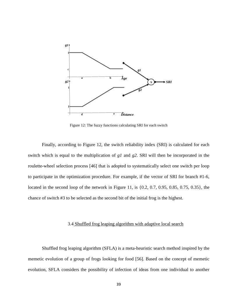
Figure 12: The fuzzy functions calculating SRI for each switch
Finally, according to Figure 12, the switch reliability index (SRI) is calculated for each
switch which is equal to the multiplication of g1 and g2. SRI will then be incorporated in the
roulette-wheel selection process [46] that is adopted to systematically select one switch per loop
to participate in the optimization procedure. For example, if the vector of SRI for branch #1-6,
located in the second loop of the network in Figure 11, is {0.2, 0.7, 0.95, 0.85, 0.75, 0.35}, the
chance of switch #3 to be selected as the second bit of the initial frog is the highest.
3.4 Shuffled frog leaping algorithm with adaptive local search
Shuffled frog leaping algorithm (SFLA) is a meta-heuristic search method inspired by the
memetic evolution of a group of frogs looking for food [56]. Based on the concept of memetic
evolution, SFLA considers the possibility of infection of ideas from one individual to another
g1
g2b
c
a
d e
f
Distance
1
1
AgeX
g1
g2
SRI
39

one in a local search area. A shuffling methodology is also permitted to make this algorithm able
for the exchange of information between local searches in order to yield a global optimum. This
algorithm combines a deterministic and random approach. The deterministic strategy forces the
method to use response surface information in order to guide the heuristic search as effective as
possible. However, the random elements result in a more robust and flexible search pattern.
In the rest of this section, at first, the concept of SFLA is briefly explained. Then, the
shortcoming of this global optimization algorithm for being applied to the network
reconfiguration problem is discussed. Finally, a systematic approach is proposed to address this
caveat.
Suppose there are several stones and a group of frogs in a swamp. The main goal of the
frogs is to find the stone with the maximum food. The frogs have the permission to communicate
with each other to improve their memes. Meme improvement is achieved by changing leaping
steps of each frog so that an individual frog's position becomes closer to the best stone.
The first step to simulate SFLA is to randomly generate a certain number of feasible
frogs as the initial population. At a later stage, the frogs are sorted in a descending order based
on their fitness values. Then, all of the frogs are divided into m memeplexes, each of which
contains n frogs. In order to classify the frogs, the first member of the sorted set is put in the first
memeplex, the second one in the second memeplex, the mth one in the mth memeplex, the
(m+1)th one in the first memeplex and so on. By partitioning the frogs, a set of “parallel frog
cultures” are created which try to move towards the main goal individually in parallel.
At the next stage, an evolutionary method is applied to the worst frog (the one with the
worst fitness value) in each memeplex to improve its position (i.e. to become closer to the stone
40

containing the maximum food). The following equations show this process that is called “local
search”:
)().( ,oldwb XXrandD −= (23)
maxmax
,, ;DDD
DXX oldwneww
≤≤−
+= (24)
where, rand() is a random number between zero and one. Xb, Xw,old and Xw,new refer to the best
frog, the current worst frog and the new frog in the corresponding memeplex, respectively. D and
Dmax stand for the step size and the maximum allowed step size. If this strategy generates a better
frog with a lower fitness value, the new frog replaces the old one. Otherwise, the same process
should be repeated with a difference that instead of using the local best frog in Equation 23 the
global best frog (i.e. the best frog in all memeplexes) should be used. If using the global best frog
does not improve the worst frog either, a new frog is generated randomly that replaces the worst
one. Finally, the entire individuals in different memeplexes are combined and all the steps are
repeated until a convergence criterion is satisfied. The final step, that is called shuffling process,
improves the meme quality and makes the cultural evolution free from any bias. In this step, all
the frogs in different memeplexes are combined together to build a united population. More
details about the implementation of SFLA can be found in [23].
The above mentioned SFLA procedure is not directly applicable to the distribution
network reconfiguration task since it does not guarantee the feasibility and radiality of the
41

generated frogs through the local search step. In other words, some generated frogs (i.e.
distribution system configurations) via Equations 23 and 24 might be: (1) infeasible; which
means the generated frog may contain bits that refer to the switches not existing in the
corresponding loop. For example, the created frog for Figure 11 is not feasible if its first bit
refers to a branch number that is located in loop #2, (2) non-radial; for example, the frog {5, 6}
generated for Figure 11 is not radial.
The most straightforward strategy to address this challenge is to repeat the local search
procedure for each memeplex and iteration of SFLA until feasible and radial (F&R)
configurations are identified. Despite of its simplicity, this process is too time-consuming for
large distribution networks and it significantly increases the computation burden of the
algorithm. Another possible simple technique to solve this problem is to assign a penalty factor
to the objective functions (refer to Equations. 2-3 and 15-16) for generated non-F&R frogs.
Applying this method still reduces the convergence speed since the optimization algorithm needs
to be executed for more iterations to learn the consequence of generating non-F&R
configurations (i.e. with higher objective values).
In this chapter a novel "adaptive local search" is proposed that automatically generates
F&R frogs in the local search step of SFLA which significantly reduces the computation burden
of the algorithm. In the proposed method a matrix called Loop-Branch Cell-Matrix (LBCM) is
introduced whose dimensions is L×L, where L represents the number of loops in the network.
Each element of LBCM contains a vector called Cell Vector (CV). The CVs located on the
diagonal components of LBCM contain the branch numbers of the corresponding loops.
However, the CVs related to the non-diagonal components of LBCM consist of the common
42
branches between the relevant loops. The procedure to implement the proposed technique is as
follows:
1) Implement Equations 23 and 24 to calculate Xw,new.
2) Repeat this process for l=1:L.
3) If the loop number (l) is more than one, go to 4. Otherwise, go to 5.
4) for m=1:l-1; if any component of LBCM(l,m) has been selected so far,
LBCM(l,l)=LBCM(l,l)- LBCM(l,m).
5) Round Xw,new (l) to the closest component of LBCM(l,l).
Once the LBCM is created, it is used to modify the output of local search of SFLA so that
any possible non-F&R configuration will be converted into an F&R configuration, which
significantly increases the speed of the optimization process.
Considering Figure 13 as an example, the LBCM has four rows and four columns. It is
assumed that the best and the worst configurations of Figure 13 are {10, 4, 16, 11} and {7, 2, 18,
10}, respectively. Applying Equations 23 and 24 to these frogs, the vector of Xw,new will be
obtained. According to Equation 25, the first generated bit of the frog is 9.6 that should be
rounded to the closest integer value corresponding to LBCM(1,1), which is CV={5,6,7,8,9,10}.
Therefore, the first modified bit becomes "10". The second bit is 2.9. The CVs of LBCM(2,2)
and LBCM(2,1) are {1,2,3,4,5,6} and {5,6}, respectively. Since any element of LBCM(2,1) has
not been selected yet, LBCM(2,2) remains unchanged and 2.9 is rounded to "3".
43

Figure 13: The sample network used to clarify the adaptive local search step
,
7 10 7 9.62 4 2 2.9
(1,4).18 16 18 17.710 11 10 10.3
T T T
w newX rand
− − = + × = −
−
(25)
The third bit is 17.7. The CVs of LBCM(3,3), LBCM(3,1) and LBCM(3,2) are
{14,15,16,17,18}, {Ø} and {17 (3), 18 (4)}, respectively. Since the branch #3 has been already
picked, LBCM(3,3) is changed into {14,15,16}. Therefore, 17.7 is rounded to "16". Finally, the
fourth bit is 10.3. The CVs of LBCM(4,4), LBCM(4,1), LBCM(4,2) and LBCM(4,3) are
{10,11,12,13}, {10}, {Ø} and {Ø}, respectively. Therefore, LBCM(4,4) should be changed into
{11,12,13} because the branch #10 was selected for the first loop. As a result, 10.3 is rounded to
"11" to create the new frog of {10, 3, 16, 11} as the output of the adaptive local search step.
It is notable that according to Equation 25 the output of the conventional local search of
SFLA is {10, 3, 18, 10} which is obviously non-radial. However, as explained above, the output
Substation
1 2
1
2
3 (17)
4 (18)
5
67
8
9
10
16
1511 12
1314
3
4
44

of the proposed adaptive local search is F&R.
3.5 Implementation
The pseudo code of the proposed fuzzy Pareto dominance adaptive shuffled frog leaping
algorithm (FPD-ASFLA) for identifying a Pareto frontier as the high-quality suboptimal network
configurations is as follows:
1) Generate the initial population of frogs using the reliability based systematic
encoding proposed in 3.3.
2) Put Iteration=1.
3) Run Newton–Raphson power flow program.
4) Calculate power loss, voltage sag and THD for each frog using Equations 2-3 &
15-16.
5) Compute the rank of each frog using Equations 21 and 22.
6) Sort the individuals in a descending order based of their rank.
7) If Iteration >1 go to 8, directly. Otherwise, save the best frog (i.e. the
configuration with the lowest rank) in the archive set (AS)) and go to 10.
8) Calculate the domination degree of each frog in population proportional to all the
frogs in AS, using Equation 21. If there is no frog in AS dominating the relevant individual
in the population, it will be added to AS as a new member. This process will be repeated
for all the frogs in population.
45

9) Compute the domination degree of each old member in AS proportional to all the
new members of AS. If there is even one new member dominating the relevant old frog, the
old individual will be removed from AS. This process will be repeated for all the old
members of AS.
10) Sort and partition all the frogs in m memeplexes based on the method presented
in 3.4.
11) Repeat the process of local search (LS) for each m memeplex, using Equations 11
and 12, until LS_Iteration=Max_ LS_Iteration. And modify the topology of each
recently created frog in this step through the presented strategy in 3.4 to develop F&R
individuals.
12) Apply the shuffling process, as it was explained in 3.4, to combine all the frogs in
different memeplexes and create a united population.
13) If Iteration = Max_Iteration, go to 14. Otherwise, Iteration= Iteration+1 and go
to 3.
14) Report all the frogs saved in the most recently AS as the suboptimal network
configurations identified by the proposed hybrid optimization algorithm. Based on the
network operational situation, the operator will decide to rely on which configuration of
the optimal Pareto frontier.
46
3.6 Simulation results and discussions
The proposed algorithm is implemented in MATLAB software on a computer with the
processor of Intel(R) Xeon(R) CPU E5-2603 0 @ 1.80 GHz. The performance of the proposed
hybrid FPD-ASFLA algorithm is demonstrated by its implementation on a 136-bus distribution
network [57], that is shown in Figure 14. The tie switches are distinguished by dash lines and red
numbers. This network contains 156 branches and 21 loops. It is assumed that one switch is
installed at each branch. It is notable that adopting the loop-based encoding strategy leads to
frogs with only 21 bits, which significantly reduces the computational burden of the optimization
algorithm compared to the case of branch-based or node-based coding techniques.
Figure 14: A 136-bus distribution network with 21 loops (Loop #16 contains branch numbers {1-7, 136, 73, 70, 63-
68, 99-101, 103-107, 110, 153, 45-47, 43, 42, 40, 39}) [57]
47

The calculated g1, g2, and SRI values (according to section 3.3) for all the switches are
presented in Figure 15. For simplicity, the length of all branches is considered to be equal. As it
can be observed, the probability of selecting switch #9 for encoding the initial frogs is much
higher than an aged switch (e.g. #8) or a switch with a more critical location (e.g. #17).
To consider nonlinear loads for the network, 19 harmonic currents as the percentage of
fundamental currents are defined for 11 buses of the system which are presented in Table 3.
Also, four points of common coupling are assumed for Bus #12, 20, 24 and 28.
Table 3: Nonlinear Load Data (Percentage of Fundamental Frequency
Bus No.
Harmonic No. 3 5 7 9 11 13 15 17 19
7 0 30 0 0 8 6.8 0 4.1 3.2
8 90 60 45 28 10 8 6 5 4
11 75 56 34 6 13 0 0 0 0
16 0 1 1 0 8 4 0 0.2 0.1
21 0 90 85 0 65 0 0 34 5
26 0 95 90 0 70 65 0 46 10
45 0 40 20 0 9 7.7 0 0.7 0.4
52 80 53 31 13 7 5.5 5 4.5 1.1
54 0 2 2 0 9 5 0 0.3 0.2
63 0 50 30 0 10 8.9 0 6.2 4.3
91 85 65 40 8 33 36 0 0 0
48
Figure 15: The determined SRI of each switch
The algorithm stops when it reaches Iteration #100 after repeating the local search
process 10 times for each iteration (i.e. LS_Iteration=10). The performance of the proposed
algorithm (FPD-ASFLA) is compared with FPD-SFLA (i.e. the proposed hybrid model without
adapting the local search step) and FPD-GA (i.e. applying the same Pareto dominance technique
to genetic algorithm). In order to provide a fair comparison, these three optimization algorithms
start the searching process from the same initial frog population.
The growing trend of the number of archive set (AS) members during the optimization
procedure is shown in Figure 16. The minor reductions observed in this figure are due to
applying step 9 in 3.5. As it can be inferred, FPD-ASFLA, FPD-SFLA and FPD-GA will identify
31, 55 and 26 non-dominated frogs in their AS after 100 iterations.
8 73 144251 17 39 63 12199
0.1
0.2
0.3
0.4
0.5
Branch Number
The
Rel
ativ
e Pr
obab
ility
of S
elec
tion
g1g2LSRI
49

Figure 16: The number of AS members
Since a number of non-dominated solutions with three fitness values (i.e. power loss,
voltage sag and THD) are identified in each iteration, the average fitness value of the updated AS
members is selected to present the progress of algorithm. The declining trend of average fitness
values for the three algorithms is depicted in Figure 17. Comparing Figures 16 and 17, it can be
realized that although FPD-SFLA has identified a higher number of non-dominated frogs, FPD-
ASFLA provides the higher qualified suboptimal solutions.
20 40 60 80 1000
10
20
30
40
50
60
Iteration
Num
ber o
f AS
Mem
bers
FPD-ASFLAFPD-SFLAFPD-GA
50
Figure 17: The declining trend of average fitness values
Table 4 provides a more detailed comparison between the performance of the mentioned
algorithms and the corresponding single models (i.e. single objective SFLA and GA). As it can
be noticed, the computational burden of FPD-ASFLA is considerably less than that of the Pareto
based models; however, single objective SFLA has the lowest operation time. On the other hand,
FPD-ASFLA has identified the configurations with the lowest power loss, voltage sag and THD
on its Pareto frontier.
0 20 40 60 80 100150
200
250
300
350
400
450
500
550
Iteration
Ave
rage
Fitn
ess
Val
ue
FPD-ASFLAFPD-SFLAFPD-GA
51
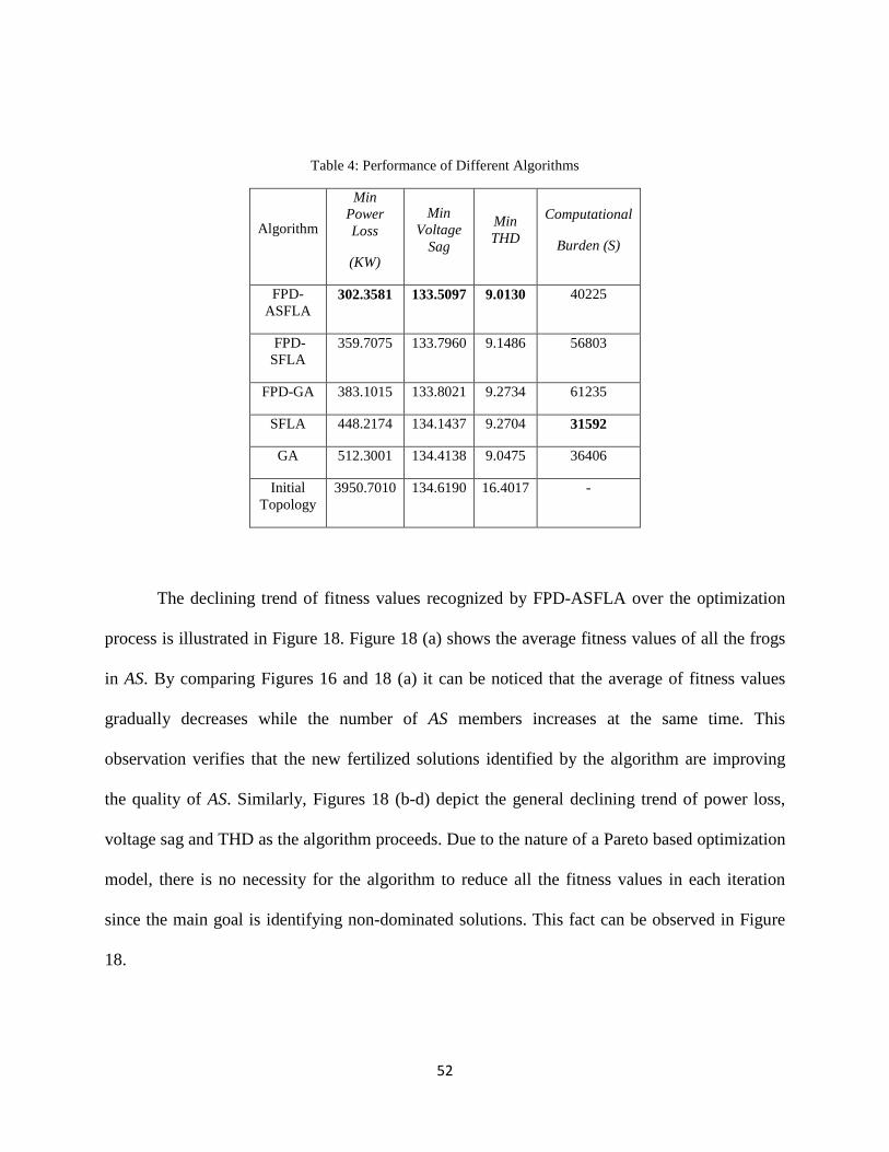
Table 4: Performance of Different Algorithms
Algorithm
Min Power Loss
(KW)
Min Voltage
Sag
Min THD
Computational
Burden (S)
FPD-ASFLA
302.3581 133.5097 9.0130 40225
FPD-SFLA
359.7075 133.7960 9.1486 56803
FPD-GA 383.1015 133.8021 9.2734 61235
SFLA 448.2174 134.1437 9.2704 31592
GA 512.3001 134.4138 9.0475 36406
Initial Topology
3950.7010 134.6190 16.4017 -
The declining trend of fitness values recognized by FPD-ASFLA over the optimization
process is illustrated in Figure 18. Figure 18 (a) shows the average fitness values of all the frogs
in AS. By comparing Figures 16 and 18 (a) it can be noticed that the average of fitness values
gradually decreases while the number of AS members increases at the same time. This
observation verifies that the new fertilized solutions identified by the algorithm are improving
the quality of AS. Similarly, Figures 18 (b-d) depict the general declining trend of power loss,
voltage sag and THD as the algorithm proceeds. Due to the nature of a Pareto based optimization
model, there is no necessity for the algorithm to reduce all the fitness values in each iteration
since the main goal is identifying non-dominated solutions. This fact can be observed in Figure
18.
52
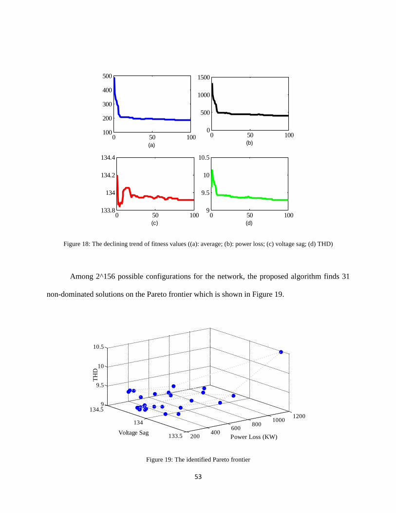
Figure 18: The declining trend of fitness values ((a): average; (b): power loss; (c) voltage sag; (d) THD)
Among 2^156 possible configurations for the network, the proposed algorithm finds 31
non-dominated solutions on the Pareto frontier which is shown in Figure 19.
Figure 19: The identified Pareto frontier
0 50 100100
200
300
400
500
(a)
0 50 1000
500
1000
1500
(b)
0 50 100133.8
134
134.2
134.4
(c)0 50 100
9
9.5
10
10.5
(d)
200 400600 800
1000 1200
133.5
134
134.59
9.5
10
10.5
Power Loss (KW)Voltage Sag
THD
53

Once the optimal Pareto frontier is identified, among the 31 candidates, the most
appropriate configurations can be selected based on the operator’s decision. For instance, four
scenarios are defined in this section as follows: (1) a configuration is desired that causes
minimum power loss; (2) a configuration is desired that causes the minimum voltage sag; (3) a
configuration is desired that causes the minimum THD; (4) a configuration is desired that causes
the minimum average of power loss, voltage sag and THD. The suboptimal frogs for the defined
scenarios will be: (1) {9, 83, 79, 84, 135, 145, 148, 90, 104, 150, 120, 141, 106, 126, 128, 7, 92,
98, 139, 96, 51}; (2) {8, 67, 78, 15, 135, 145, 148, 90, 147, 150, 118, 141, 110, 123, 154, 47, 92,
151, 139, 142, 48}; (3) {9, 15, 79, 84, 135, 145, 148, 90, 104, 150, 119, 141, 106, 126, 128, 7,
92, 98, 139, 96, 51}; (4) {9, 83, 79, 84, 135, 145, 148, 90, 104, 150, 119, 141, 106, 126, 128, 7,
92, 98, 139, 96, 51}.
Table 5 compares the impact of conventional and the proposed reliability based encoding
approaches on the quality of the identified Pareto frontier. According to this table, if the
proposed encoding method is used, the number of risky switching that is scheduled in the
suboptimal configurations significantly reduces. It is notable that, in Table 5, the change in the
status of a given switch is considered as a risky operation if the associated SRI for the switch is
less than 0.2.
54
Table 5: The Effect of the Proposed Reliability-based Encoding Strategy on the Performance of the Algorithm
Power Loss
(KW)
Voltage Sag
THD High Risky
Operations
Proposed Encoding
432.85 134.09 9.28 9
Conventional Encoding
430.07 134.83 9.65 34
3.7 Summary
In this chapter, a novel hybrid optimization algorithm based on the combination of fuzzy
Pareto dominance (FPD) and shuffled frog leaping algorithm (SFLA) is proposed to solve the
multi-objective optimization problem of distribution network reconfiguration with the purpose of
minimizing power loss, voltage sag and THD. It identifies a Pareto frontier as the non-dominated
suboptimal configurations. The local search step of SFLA is customized for the application of
power system reconfiguration that significantly reduces the computational burden of the
algorithm. A reliability based encoding strategy is also developed that selects more reliable
solutions as the start point of the optimization procedure. The performance of the proposed
hybrid optimization algorithm is demonstrated by its implementation on a 136-bus distribution
network. The simulation results verify that the proposed optimization algorithm not only is much
faster in convergence compared to the similar Pareto based models but also it identifies more
fertilized solutions. It is also demonstrated that the proposed reliability based initial encoding
leads to more reliable solutions found by the algorithm after 100 iterations.
55

CHAPTER FOUR: OPTIMAL DISTRIBUTION NETWORK
RECONFIGURATION USING DYNAMIC FUZZY BASED GENETIC
ALGORITHM
4.1 Overview of genetic algorithm
The three main optimization tools employed in engineering problems are neural networks
(NNs), machine learning and evolutionary computation (EC). GA is known as the most
prominent and popular member of EC family. GA performs based on the idea of natural selection
to evolve a population of chromosomes as the candidate solutions to a given problem using its
operators that are selection, crossover, and mutation. According to the principle of "survival of
the fittest", the first operator selects the chromosomes based on their fitness values to participate
in the reproduction of the next generation. The second operator changes subparts of each two
chromosomes, selected by the first operator, to produce two new individuals. In order to
maintain the genetic diversity of a population, mutation is utilized to alter one or more gene
values of each chromosome that produces a new individual for the next generation. More details
about the concept of GA and its implementation can be found in [58]. The procedure of solving
the reconfiguration optimization problem by GA is explained as follows:
Step 1) Generate N chromosomes randomly as an initial population.
Step 2) Run the load flow program.
Step 3) Compute the fitness value of each individual.
Step 4) Select N chromosomes based on the adopted selection strategy.
56

Step 5) For each two selected chromosomes, generate a value between zero and one,
randomly. If this value is less than the crossover probability, apply the adopted crossover
strategy to the pair to create two new chromosomes which replace the two old ones. Otherwise,
the pair remains unmodified.
Step 6) For each chromosome, generate a value between zero and one, randomly. If this
value is less than the mutation probability, apply the mutation strategy on the chromosome to
produce a new individual. Otherwise, the chromosome is directly transferred to the next step
without any change.
Step 7) If the stopping criterion is satisfied, print the chromosome with the minimum
fitness value as the final solution and go to step 8. Otherwise, go to step 2.
Step 8) Finish.
4.2 Determining crossover and mutation parameters
The crossover and mutation parameters, which are presented as Pc and Pm, respectively,
indicate the probabilities based on which crossover and mutation occurs. The efficient
performance of GA critically originates from a successful crossover and mutation. Therefore, an
accurate technique to determine Pm and Pc plays a significant and undeniable role in the behavior
of GA [59]. The value of Pc controls the speed of exploiting process in identifying the best
answer in a local area. On the other hand, the value of Pm adjusts the speed of algorithm in
exploring new regions. Therefore, a meaningful relationship between crossover and mutation
57

probabilities is necessary to prevent the algorithm from falling into local optimums, which is the
result of a weak exploration, or from having a low convergence speed, that is the consequence of
a poor exploitation.
Conventionally, trial and error procedures were used by researchers to find fixed values
for Pc and Pm. For instance, trial and error experiments are utilized in [60] to determine the fixed
Pc and Pm values of a GA that is employed to tune the node connection weights of an artificial
neural network (ANN) in load forecasting. Despite of their simplicity, there is a main
disadvantage accompanied with these trial and error techniques. As the algorithm proceeds, the
optimal contribution rates of crossover and mutation varies that brings about the necessity of
having different crossover and mutation probabilities for different chromosomes and different
generations [61]. However, these trial and error methods can provide only one single Pc and Pm
for all the chromosomes in different generations. For this reason, a self-adaptive GA is proposed
in this chapter, which is able to automate the parameters setting process and update them
dynamically as the evolution of chromosomes goes forward.
In this chapter, the concept of fuzzy membership functions is utilized to introduce a
dynamic strategy for determining Pc and Pm. The process is elaborated in this section for the
mutation operator. The first function, f1, assigns a fuzzy membership value between zero and
one, shown as p1, to the chromosome based on the distance of its fitness value from the best
fitness value in the same generation. If the chromosome is close to the best individual, f1 assigns
a lower value to the chromosome to decrease the probability of mutation and increase the
survival possibility of that chromosome in the next generation. On the other hand, if the
chromosome is far from the best individual, f1 assigns a higher value to the chromosome to
58

increase the mutation probability with the hope of producing a new chromosome with a better
fitness value. The first fuzzy function is depicted in Figure 20.
Figure 20: The fuzzy function determining P1
The second function, f2, assigns a fuzzy value, shown as p2, to the chromosome based on
the distance of the average fitness value of all the chromosomes in the same generation from the
best fitness value. It is notable that the calculated fuzzy membership value is equal for all the
chromosomes in the same generation. If the average fitness value is close to the best individual's
fitness, it means all the chromosomes in the population are converging to one individual which
increases the risk of falling into a local optimum. As a result, f2 assigns a higher value to all the
chromosomes to raise the mutation probability and explore new regions. On the other hand, if the
average fitness value is far from the best fitness value, it means the chromosomes are exploring
too much and they do not consider the existing optimum in their locality. For this reason, f2
determines a lower value for p2 to decrease the mutation probability and gain up the speed of
exploiting process. The second fuzzy function is illustrated in Figure 21.
0 Minfit b Maxfit
a
1
Fitness Value
f1(F
itnes
s)=P
1
59
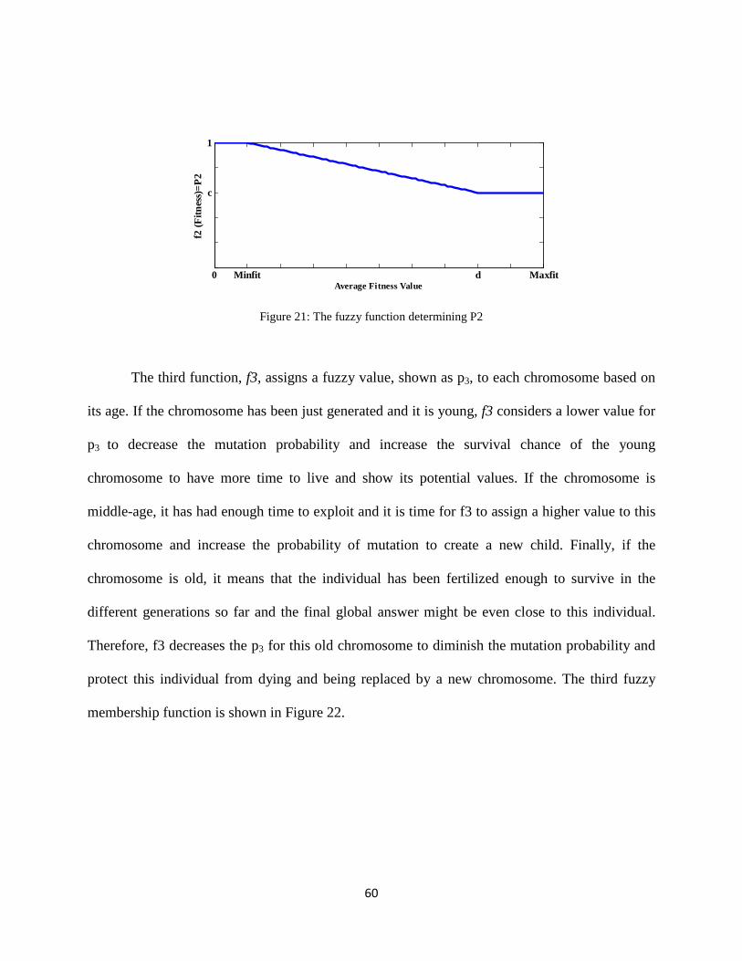
Figure 21: The fuzzy function determining P2
The third function, f3, assigns a fuzzy value, shown as p3, to each chromosome based on
its age. If the chromosome has been just generated and it is young, f3 considers a lower value for
p3 to decrease the mutation probability and increase the survival chance of the young
chromosome to have more time to live and show its potential values. If the chromosome is
middle-age, it has had enough time to exploit and it is time for f3 to assign a higher value to this
chromosome and increase the probability of mutation to create a new child. Finally, if the
chromosome is old, it means that the individual has been fertilized enough to survive in the
different generations so far and the final global answer might be even close to this individual.
Therefore, f3 decreases the p3 for this old chromosome to diminish the mutation probability and
protect this individual from dying and being replaced by a new chromosome. The third fuzzy
membership function is shown in Figure 22.
0 Minfit d Maxfit
c
1
Average Fitness Value
f2 (F
itnes
s)=P
2
60

Figure 22: The fuzzy function determining P3
Therefore, the probability of mutation for each chromosome is calculated as follows:
ant 1 2 3m constP P P P P= × × × (26)
where, in Figures 20-22 and Equation 26 the fixed values of a, b, c, d, e, f, g and Pconstant are
determined through a trial and error procedure. The same process can be repeated for the
crossover operator with only one difference that the x-axis in Figure 20 and 22 will stand for the
average fitness and the average age of the corresponding pair, respectively.
4.3 Simulation results and discussions
The presented method is developed in MATLAB and the simulation process is done on a
computer with the processor of Intel(R) Xeon(R) CPU E5-2603 0 @ 1.80 GHz. The algorithm is
0 f g MaxAge
e
1
Age
f3(F
itnes
s)=P
3
61

tested on a 33-bus radial distribution network [62] that is shown in Figure 23. It contains 32
sectionalizing switches and five tie lines.
Figure 23: Case study [62]
The chromosome encoding strategy adopted in this chapter is the same loop-based
encoding method elaborated in Chapter 3. The utilized coding technique is much faster and more
computationally efficient than the branch-based and node-based strategies which would bring
about the chromosomes with 37 and 33 genes, which are the number of branches and nodes,
respectively. For instance, the generated chromosome Ch={33, 34, 35, 36, 37} represents the
18
21
32
1
4
5
6
7
8
9
10
11
12
13
14
15
16
17
24
25
19
20
21
22
26
27
28
29
30
31
32
33
33
3
4
5
6
7
8
9
10
11
12
13
14
15
16
17
21
19
20
18
22
23
2425
26
27
28
29
30
31
32
34
35
36
37
62

initial configuration (see Figure 23) in which all the branches are closed except the lines 33, 34,
35, 36 and 37. As can be inferred, the generated individual refers to a radial network since each
of the five open branches corresponds to one separate loop number. Utilizing the loop-based
encoding technique, GA is employed to randomly create N initial chromosomes signifying N
radial networks. N is the number of population that is assumed to be 100 in the simulation. Then,
load flow is run to compute the fitness value, which is the total power loss, for each
configuration. At a later stage, the roulette wheel selection strategy [58] is adopted to select the
more fertilized chromosomes with lower fitness values (i.e. lower total power losses). However,
the less qualified individuals still have a low chance to participate in the next generation and
increase the diversity.
Afterwards, the two point crossover technique is applied on the selected individuals.
Adopting this method, a value is selected randomly between zero and one for each two
chromosomes. If the random value is higher than the crossover probability, the two individuals
survive and will transfer to the next step without any modification. Otherwise, two points are
chosen randomly for each two chromosomes and the relevant genes between those two points are
exchanged between the two individuals to produce two new children. And the generated children
take part in the next step instead of their parents. Then, the chromosomes are mutated to
guarantee a diverse population. For this purpose, a random value between zero and one is
selected for each individual. If the value is less than the mutation probability, one of the genes of
the chromosome is selected and its value will change. Since the non-radial configurations are not
desirable, another branch from the same loop is randomly selected to replace the chosen gene.
For instance, if the gene 33 (i.e. Branch #33) in Ch is chosen to be mutated, one of the branches
63
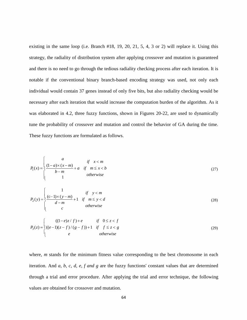
existing in the same loop (i.e. Branch #18, 19, 20, 21, 5, 4, 3 or 2) will replace it. Using this
strategy, the radiality of distribution system after applying crossover and mutation is guaranteed
and there is no need to go through the tedious radiality checking process after each iteration. It is
notable if the conventional binary branch-based encoding strategy was used, not only each
individual would contain 37 genes instead of only five bits, but also radiality checking would be
necessary after each iteration that would increase the computation burden of the algorithm. As it
was elaborated in 4.2, three fuzzy functions, shown in Figures 20-22, are used to dynamically
tune the probability of crossover and mutation and control the behavior of GA during the time.
These fuzzy functions are formulated as follows.
1(1 ) ( )( )
1
a if x ma x mP x a if m x bb m
otherwise
< − × −= + ≤ <−
(27)
2
1(c 1) ( )( ) 1
if y my mP y if m y d
d motherwisec
< − × −= + ≤ <−
(28)
3
((1 ) / ) 0( ) (( 1)( ) / ( )) 1
e z f e if z fP z e z f g f if f z g
e otherwise
− + ≤ <= − − − + ≤ <
(29)
where, m stands for the minimum fitness value corresponding to the best chromosome in each
iteration. And a, b, c, d, e, f and g are the fuzzy functions' constant values that are determined
through a trial and error procedure. After applying the trial and error technique, the following
values are obtained for crossover and mutation.
64
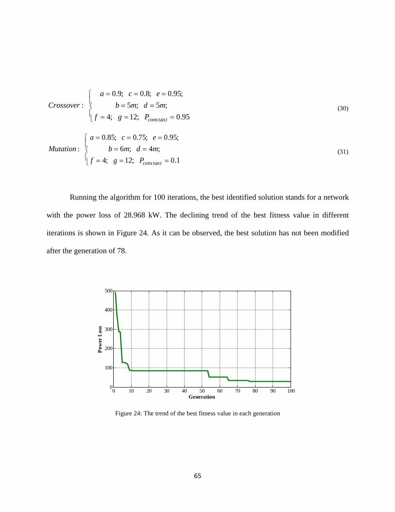
tan
0.9; 0.8; 0.95;: 5 ; 5 ;
4; 12; 0.95cons t
a c eCrossover b m d m
f g P
= = = = = = = =
(30)
tan
0.85; 0.75; 0.95;: 6 ; 4 ;
4; 12; 0.1cons t
a c eMutation b m d m
f g P
= = = = = = = =
(31)
Running the algorithm for 100 iterations, the best identified solution stands for a network
with the power loss of 28.968 kW. The declining trend of the best fitness value in different
iterations is shown in Figure 24. As it can be observed, the best solution has not been modified
after the generation of 78.
Figure 24: The trend of the best fitness value in each generation
0 10 20 30 40 50 60 70 80 90 1000
100
200
300
400
500
Generation
Pow
er L
oss
65
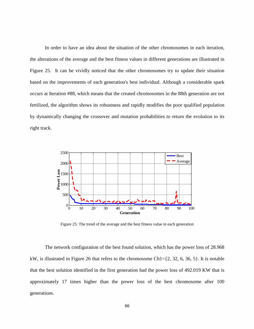
In order to have an idea about the situation of the other chromosomes in each iteration,
the alterations of the average and the best fitness values in different generations are illustrated in
Figure 25. It can be vividly noticed that the other chromosomes try to update their situation
based on the improvements of each generation's best individual. Although a considerable spark
occurs at Iteration #88, which means that the created chromosomes in the 88th generation are not
fertilized, the algorithm shows its robustness and rapidly modifies the poor qualified population
by dynamically changing the crossover and mutation probabilities to return the evolution to its
right track.
Figure 25: The trend of the average and the best fitness value in each generation
The network configuration of the best found solution, which has the power loss of 28.968
kW, is illustrated in Figure 26 that refers to the chromosome Ch1={2, 32, 6, 36, 5}. It is notable
that the best solution identified in the first generation had the power loss of 492.019 KW that is
approximately 17 times higher than the power loss of the best chromosome after 100
generations.
0 10 20 30 40 50 60 70 80 90 1000
500
1000
1500
2000
2500
Generation
Pow
er L
oss
BestAverage
66
Figure 26: The final solution
A comparison between each branch's power loss of the best identified solution in the first
and the final generation is provided in Figure 27. As it can be gathered from the figure, the final
solution dramatically wastes less amount of power in all the branches, except Branch #16,
compared to the best chromosome identified in the first generation.
18
21
3
2
1
4
5
6
7
8
9
10
11
12
13
14
15
16
17
24
25
19
20
21
22
26
27
28
29
30
31
32
33
33
3
4
5
6
7
8
9
10
11
12
13
14
15
16
17
21
19
20
18
22
23
2425
26
27
28
29
30
31
32
34
35
36
37
67
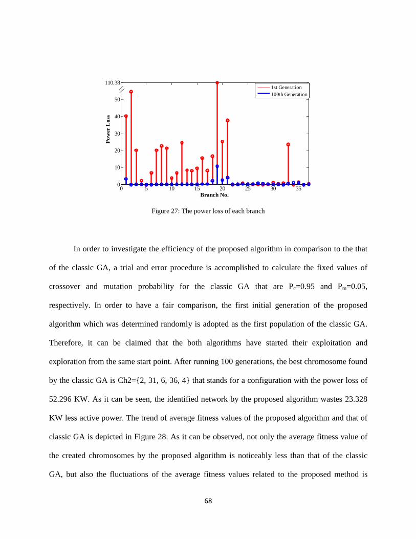
Figure 27: The power loss of each branch
In order to investigate the efficiency of the proposed algorithm in comparison to the that
of the classic GA, a trial and error procedure is accomplished to calculate the fixed values of
crossover and mutation probability for the classic GA that are Pc=0.95 and Pm=0.05,
respectively. In order to have a fair comparison, the first initial generation of the proposed
algorithm which was determined randomly is adopted as the first population of the classic GA.
Therefore, it can be claimed that the both algorithms have started their exploitation and
exploration from the same start point. After running 100 generations, the best chromosome found
by the classic GA is Ch2={2, 31, 6, 36, 4} that stands for a configuration with the power loss of
52.296 KW. As it can be seen, the identified network by the proposed algorithm wastes 23.328
KW less active power. The trend of average fitness values of the proposed algorithm and that of
classic GA is depicted in Figure 28. As it can be observed, not only the average fitness value of
the created chromosomes by the proposed algorithm is noticeably less than that of the classic
GA, but also the fluctuations of the average fitness values related to the proposed method is
0 5 10 15 20 25 30 350
10
20
30
40
50
110.38
Branch No.
Pow
er L
oss
1st Generation100th Generation
68

considerably less. It means that the presented dynamic GA with fuzzy crossover and mutation is
more robust than the classic GA. Moreover, the chromosomes produced in each generation of the
proposed model are more reliable since their power losses are significantly less than that of the
configurations identified by the classic GA.
Figure 28: The trend of average fitness values
4.4 Summary
In this chapter, a dynamic fuzzy-based GA is successfully applied to solve the
optimization problem of distribution network reconfiguration with the objective function of
minimizing total power loss in the system. In order to dynamically tune the probability of
crossover and mutation, three fuzzy functions are defined based on the situation of each
chromosome, the situation of all the individuals in a population, and finally the age of each
chromosome. Simulations of the proposed algorithm are carried on a 33-bus distribution network
and the results are compared with the efficiency of the classic GA that utilizes fixed parameters
0 10 20 30 40 50 60 70 80 90 1000
500
1000
1500
2000
2500
Generation
Ave
rage
Fitn
ess
Classic GAProposed Algorithm
69

for the operators of crossover and mutation. The simulation results demonstrate the more
robustness and reliability of the proposed algorithm.
70
CHAPTER FIVE: THE IMPACT OF DISTRIBUTED GENERATION
INTEGRATION ON OPTIMAL DISTRIBUTION NETWORK
RECONFIGURATION
5.1 Methodology
As it was explained in Chapter 3, Shuffled frog leaping algorithm (SFLA) is a meta-
heuristic optimization model that mimics the memetic evolution of a group of frogs looking for
the stone containing the maximum food in a swamp. In this chapter the concept of Pareto
dominance is considered within the structure of SFLA to develop a multi-objective global
optimization model discovering a set of non-dominated solutions located on the optimal Pareto
frontier. Figure 29 shows the flowchart of the presented reconfiguration optimization algorithm.
More explanations about this flowchart will be provided in the rest of this section.
71
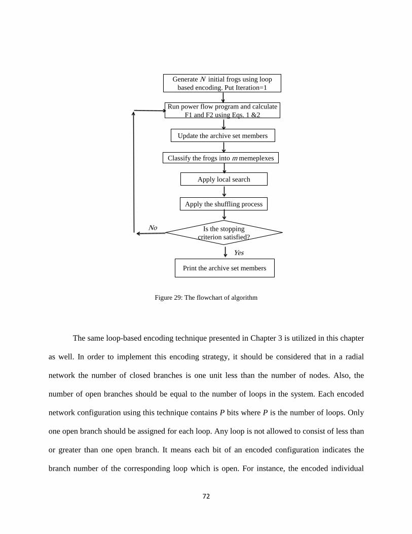
Figure 29: The flowchart of algorithm
The same loop-based encoding technique presented in Chapter 3 is utilized in this chapter
as well. In order to implement this encoding strategy, it should be considered that in a radial
network the number of closed branches is one unit less than the number of nodes. Also, the
number of open branches should be equal to the number of loops in the system. Each encoded
network configuration using this technique contains P bits where P is the number of loops. Only
one open branch should be assigned for each loop. Any loop is not allowed to consist of less than
or greater than one open branch. It means each bit of an encoded configuration indicates the
branch number of the corresponding loop which is open. For instance, the encoded individual
Generate N initial frogs using loop based encoding. Put Iteration=1
Run power flow program and calculate F1 and F2 using Eqs. 1 &2
Update the archive set members
Classify the frogs into m memeplexes
Apply local search
Apply the shuffling process
Is the stopping criterion satisfied?
Print the archive set members
Yes
No
72

(i.e. frog) for the network topology shown in Figure 30, which contains 10 nodes, 9 closed
branches and 3 loops, is F={10, 4, 11}.
Figure 30: A radial network with three loops
The archive set (AS) contains the suboptimal non-dominated solutions during the
optimization process. For example, Fig. 31a. shows the AS members found at iteration T. As it
can be seen, any frog in this set is not able to dominate any other member of AS. At each
iteration AS members should be updated in two steps: (1) The new generated frogs which are not
dominated by the current AS members should be added to the Pareto frontier. As it can be
realized from Figure 31b., the frogs z, m and n are the new AS members which are identified at
iteration T+1. (2) The old AS members which are dominated by the new AS members should be
Substation
1 2
1
2
3 4
5
67
8
9
10
3
11 12
73

removed from the Pareto frontier. As it can be gathered from Figure 31c, the frogs x and y which
are dominated by the new members z, m and n are deleted from the archive set.
Figure 31: Updating the archive set members
Different methods can be adopted to classify the encoded frogs (i.e. network
configurations) into m memeplexes. In this work, a fuzzy based strategy is presented to assign
one single fitness value to each frog as a criterion of selection for classifying. The two objective
functions defined for the algorithm to be optimized are voltage drop and voltage sag which are
formulated in Equations 4 and 15. As it is shown in Figure 32, two fuzzy values are assigned to
these objective values using the trapezoidal fuzzy functions. The multiplication of these fuzzy
values will yield the fitness value of the corresponding frog. At the next stage, the frogs should
F1
F2
x yz
F1
F2
m n
z
F1
F2
m n
a b
c
xy
74

be classified in different memeplexes. Roulette wheel method is employed for this purpose. All
the memeplexes should contain the same number of frogs and they should be prepared fairly
consisting of less fertilized and more fertilized frogs. That is why at the beginning step the first
member of each memeplex should be selected from the roulette wheel so that, most likely, the
frogs with higher fitness values will be chosen. When the first members of all the memeplexes
are selected, this process will be repeated to determine the second members of each memeplex,
and so on. It should be emphasized that each selected frog should be taken out and it will not be
put back in the roulette wheel for further selections.
Figure 32: Determining the fitness fuzzy value for classification
f1
f2b
c
a
d e
f
Voltage Sag
1
1
Voltage DropX
f1
f2
F
75

Local search is an evolutionary method that is repetitively applied to each memeplex to
improve the worst frogs of the corresponding memeplex. Using Equations 23 and 24, the best
and worst frog in the memeplex are used to generate a new frog.
If the new frog dominates the worst frog, it will be replaced by Xw,old. Otherwise, this
process will be repeated with the difference that instead of Equation 23, Equation 32 will be used
in which the best frog among all the memeplexes (i.e. Xg) will be employed to generate the new
frog. If the new developed frog cannot still dominate the older worst frog (i.e. Xw,old) in the
memeplex, another frog will be generated randomly to be replaced by the worst frog. It is notable
that the worst frog is dominated by the new one when its voltage drop and voltage sag values are
higher than that of the new frog. Repeating this evolutionary process for each memeplex, the
frogs will be improved locally.
)().( ,oldwg XXrandD −= (32)
At the end of each iteration, shuffling process will be applied to make the cultural
evolution free from any bias. After improving the worst frogs by Local Search, shuffling
processor will combine all the frogs in different memeplexes to develop a united population.
76
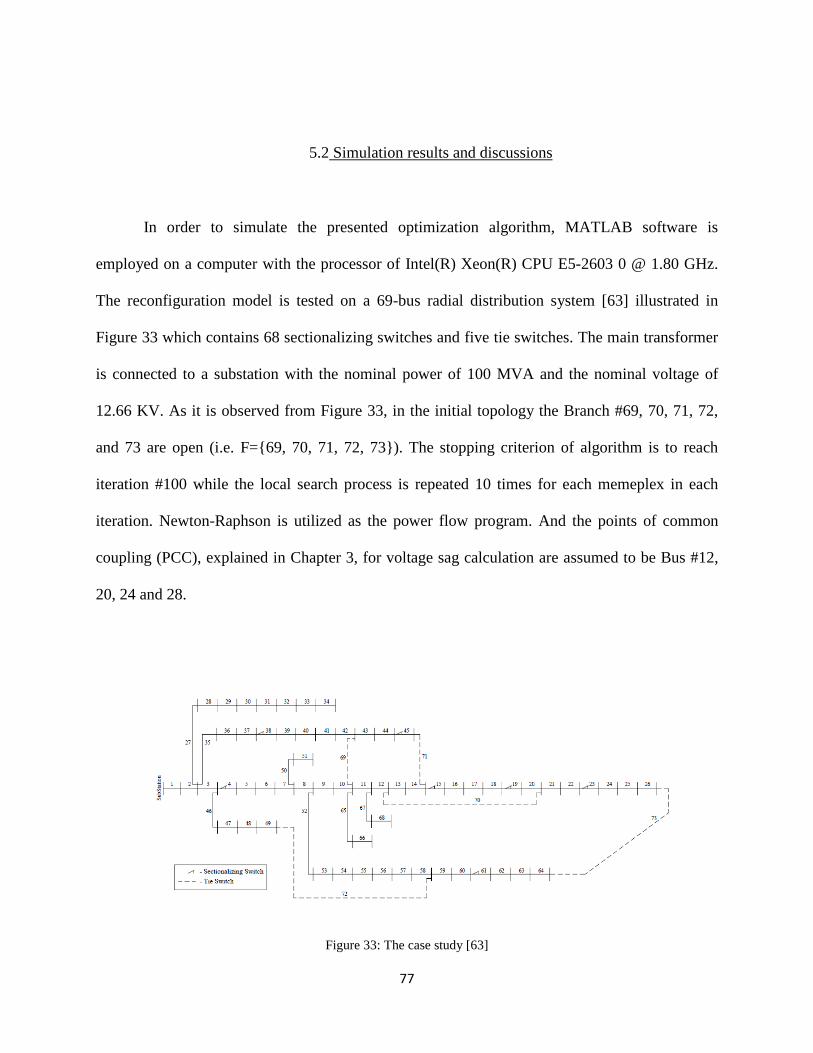
5.2 Simulation results and discussions
In order to simulate the presented optimization algorithm, MATLAB software is
employed on a computer with the processor of Intel(R) Xeon(R) CPU E5-2603 0 @ 1.80 GHz.
The reconfiguration model is tested on a 69-bus radial distribution system [63] illustrated in
Figure 33 which contains 68 sectionalizing switches and five tie switches. The main transformer
is connected to a substation with the nominal power of 100 MVA and the nominal voltage of
12.66 KV. As it is observed from Figure 33, in the initial topology the Branch #69, 70, 71, 72,
and 73 are open (i.e. F={69, 70, 71, 72, 73}). The stopping criterion of algorithm is to reach
iteration #100 while the local search process is repeated 10 times for each memeplex in each
iteration. Newton-Raphson is utilized as the power flow program. And the points of common
coupling (PCC), explained in Chapter 3, for voltage sag calculation are assumed to be Bus #12,
20, 24 and 28.
Figure 33: The case study [63]
77

To study the effect of DG integration, the optimization method is implemented in three
different scenarios as is described in Table 6. It is notable that the power factor of all the
installed DG units is 0.8 lag.
Table 6: The Description of Different Scenarios
No. DG units Location (Bus No.) Power (KVA)
Scenario #1 0 - -
Scenario #2 5 11, 21, 50, 55, 61 80, 50, 150, 10, 500
Scenario #3 10 7, 11, 12, 21, 49, 50, 55, 61, 64, 65
15, 80, 80, 50, 150, 150, 10, 500, 100, 30
The number of non-dominated solutions (i.e. the archive set’s frogs) increases as the
algorithm proceeds since it identifies a higher number of suboptimal configurations located on
the Pareto frontier. This growing trend for different scenarios is compared in Figure 34. As it is
observed from the figure, approximately, the same number of suboptimal solutions is identified
by the algorithm after 100 iterations for the three cases.
78

Figure 34: The number of AS members found by the algorithm
The first defined objective function is voltage drop. In order to present the fluctuations of
this fitness value during the optimization process, the average voltage drop of all the non-
dominated solutions is recorded as the average voltage drop of each iteration. Figure 35 provides
a comparison among the declining trends of average voltage drop for three scenarios. This
observation verifies that the integration of DG units to the network will improve the performance
of optimization algorithm to identify more high-quality suboptimal solutions with less values of
voltage drop.
10 20 30 40 50 60 70 80 90 1000
5
10
15
20
25
Iteration
No.
Non
-dom
inat
ed S
olut
ions
Sc#1Sc#3Sc#2
79

Figure 35: The declining trend of average voltage drop
The second objective function defined for the algorithm is voltage sag. As different non-
dominated solutions are found in each iteration, the average voltage sag of suboptimal solutions
is recorded to stand for the second fitness value of the relevant iteration. The declining trends of
average voltage sag for three scenarios during the optimization process are compared in Figure
36. As it is demonstrated, the presence of DG units in the network will make the optimization
algorithm more efficient in finding the topologies with less voltage sag values.
0 10 20 30 40 50 60 70 80 90 100
0.8
1
1.2
1.4
0.7
Iteration
Ave
rage
Vol
tage
Dro
p (p
u)
Sc#1Sc#3Sc#2
80

Figure 36: The declining trend of average voltage sag
As it was presented in Figure 34, the algorithm finds approximately the same number of
non-dominated solutions after 100 iterations for different scenarios. These suboptimal network
configurations are located on Pareto frontiers which are illustrated together in Figure 37. As it
was expected, the higher number of DG units in the system will help the reconfiguration model
identify more high-quality Pareto frontiers with the lower values of voltage drop and voltage sag.
0 10 20 30 40 50 60 70 80 90 10024
25
26
27
28
29
30
31
Iteration
Ave
rage
Vol
tage
Sag
Sc#1Sc#3Sc#2
81

Figure 37: The frontiers identified by the algorithm for three scenarios
Table 7 presents the configurations with the lowest value of voltage drop on the identified
frontiers. The second row of this table indicates the open switches of each topology.
Table 7: The Configurations with the Lowest Voltage Drop
Initial Scenario #1 Scenario #2 Scenario #3
Configuration 69,70,71,72,73 10, 20, 13, 58, 26 69, 20, 13, 58, 64 69, 19, 13, 58, 64
Voltage Drop 1.8460 1.0637 0.6961 0.6236
The voltage profiles of the network topologies presented in Table 7 are depicted in Figure
38. As it was expected, running the optimization algorithm even in the absence of DG units will
lead to a more high-quality suboptimal configuration with an improved voltage profile (refer to
the green and red profiles in Figure 38). Also, it is verified that Sc#3 with the highest number of
0.7 0.8 0.9 1 1.1 1.2 1.3 1.422
24
26
28
30
Voltage Drop
Vol
tage
Sag
Sc#1Sc#3Sc#2
82
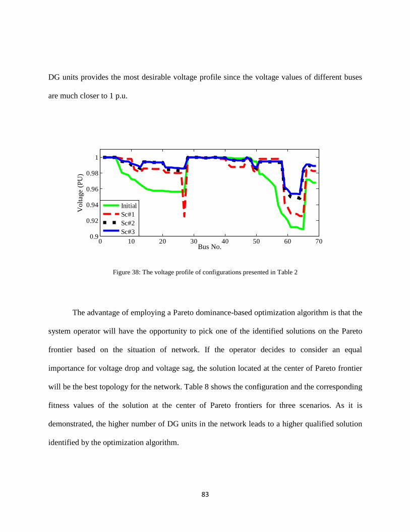
DG units provides the most desirable voltage profile since the voltage values of different buses
are much closer to 1 p.u.
Figure 38: The voltage profile of configurations presented in Table 2
The advantage of employing a Pareto dominance-based optimization algorithm is that the
system operator will have the opportunity to pick one of the identified solutions on the Pareto
frontier based on the situation of network. If the operator decides to consider an equal
importance for voltage drop and voltage sag, the solution located at the center of Pareto frontier
will be the best topology for the network. Table 8 shows the configuration and the corresponding
fitness values of the solution at the center of Pareto frontiers for three scenarios. As it is
demonstrated, the higher number of DG units in the network leads to a higher qualified solution
identified by the optimization algorithm.
0 10 20 30 40 50 60 700.9
0.92
0.94
0.96
0.98
1
Bus No.
Vol
tage
(PU
)
InitialSc#1Sc#2Sc#3
83

Table 8: The Configurations Located at the Center of Pareto Frontiers
Initial Scenario #1 Scenario #2 Scenario #3
Configuration 69,70,71,72,73 10, 19, 12, 58, 25 69, 19, 12, 58, 26 69, 19, 12, 58, 25
Voltage Drop 1.8460 1.1305 0.7693 0.7406
Voltage Sag 30.9650 26.8401 24.8758 24.3895
As it was gathered from Figure 34, the optimization algorithm identifies 24 non-
dominated solutions for Scenario #3, whose fitness values are depicted in Figure 37. Table 9
presents these network topologies. The number in each column indicates the branch number
which is open in the corresponding loop.
84

Table 9: The Suboptimal Configurations Identified for Scenario #3
Solution Loop#1 Loop#2 Loop#3 Loop#4 Loop#5
1 69 18 12 58 26
2 69 18 12 58 23
3 69 18 12 58 25
4 69 18 12 57 25
5 69 17 12 58 24
6 69 17 12 57 24
7 69 14 12 57 22
8 69 19 13 58 26
9 69 19 12 58 26
10 69 20 13 58 73
11 69 19 12 58 24
12 69 19 12 58 25
13 69 20 14 58 26
14 69 20 13 58 26
15 69 19 12 58 23
16 69 20 12 58 26
17 69 20 12 58 25
18 69 20 12 58 24
19 69 20 13 58 23
20 69 20 12 58 23
21 69 70 12 58 23
22 69 19 13 58 64
23 69 20 13 58 64
24 69 19 12 58 64
85

5.3 Summary
The Pareto-based global optimization algorithm which was proposed in Chapter 3 has
been improved in this chapter to solve the multi-objective problem of distribution system
reconfiguration with the purpose of optimizing voltage profile and voltage sag. The optimization
method utilizes a Pareto dominance technique to recognize non-dominated solutions identified
by a shuffled frog leaping algorithm (SFLA) which is adapted in the encoding and partitioning
steps. A fuzzy logic is introduced in the partitioning step of SFLA based on the values of voltage
drop and voltage sag in order to provide a more accurate criterion for the classification of frogs.
The proposed optimization algorithm is implemented in the presence of DGs to step toward the
integration of smart grids embedded in the structure of conventional power systems. The
simulation results verify that increasing the number and size of added DG units in the network
will improve the efficiency of the optimization algorithm to identify higher qualified suboptimal
solutions for the system.
86
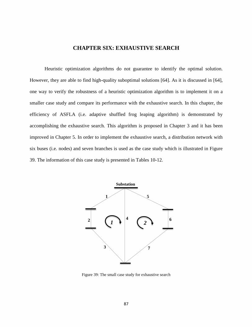
CHAPTER SIX: EXHAUSTIVE SEARCH
Heuristic optimization algorithms do not guarantee to identify the optimal solution.
However, they are able to find high-quality suboptimal solutions [64]. As it is discussed in [64],
one way to verify the robustness of a heuristic optimization algorithm is to implement it on a
smaller case study and compare its performance with the exhaustive search. In this chapter, the
efficiency of ASFLA (i.e. adaptive shuffled frog leaping algorithm) is demonstrated by
accomplishing the exhaustive search. This algorithm is proposed in Chapter 3 and it has been
improved in Chapter 5. In order to implement the exhaustive search, a distribution network with
six buses (i.e. nodes) and seven branches is used as the case study which is illustrated in Figure
39. The information of this case study is presented in Tables 10-12.
Figure 39: The small case study for exhaustive search
Substation
1 2
5
6
3
4
1
2
7
87
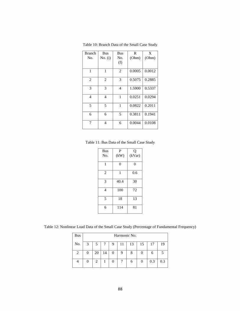
Table 10: Branch Data of the Small Case Study
Branch No.
Bus No. (i)
Bus No. (f)
R (Ohm)
X (Ohm)
1 1 2 0.0005 0.0012
2 2 3 0.5075 0.2885
3 3 4 1.5900 0.5337
4 4 1 0.0251 0.0294
5 5 1 0.0822 0.2011
6 6 5 0.3811 0.1941
7 4 6 0.0044 0.0108
Table 11: Bus Data of the Small Case Study
Bus No.
P (kW)
Q (kVar)
1 0 0
2 1 0.6
3 40.4 30
4 100 72
5 18 13
6 114 81
Table 12: Nonlinear Load Data of the Small Case Study (Percentage of Fundamental Frequency)
Bus
No.
Harmonic No.
3 5 7 9 11 13 15 17 19
2 0 20 14 0 9 8 0 6 5
4 0 2 1 0 7 6 0 0.3 0.3
88

It is notable that the exhaustive search evaluates all the possible configurations (i.e.
27=128) and reports the configuration with the best fitness value. And at the next step, the
proposed heuristic algorithm (i.e. ASFLA) is simulated to identify the high-quality solutions
after 80 iterations. The initial population contains 60 frogs (i.e. 60 initial configurations selected
randomly). The number of memeplexes is assumed to be three. And for each iteration, the local
search step is repeated for 10 times.
As for the first scenario, the exhaustive search is implemented to find the configuration
with minimum power loss. The identified configuration is {2,4} where the Branch #2 and
Branch #4 are open. After running the proposed ASFLA, it is observed that the same
configuration is found after 80 iterations which is depicted in Figure 40.
Figure 40: The configuration with minimum power loss
62
Substation
1 2
5
3
4
1
7
89

Regarding the second and third scenarios, voltage sag and THD are defined, respectively,
as the objective functions. The simulation results verify that the same configurations are
identified by exhaustive search and the proposed heuristic algorithm for these scenarios as well.
The found solutions for Scenario #1 and Scenario #2 are {1,4} and {2,5}, respectively, which are
shown in Figure 41.
(a) (b)
Figure 41: The configurations with (a): minimum voltage sag and (b): minimum THD
It should be emphasized that the presented observation does not guarantee that the
proposed heuristic algorithm will have the same efficiency for a distribution system with 3000
branches (23000 possible configurations). However, it shows that the proposed ASFLA will
identify high-quality suboptimal solutions. Once again, it should be mentioned that the declining
62
Substation
1 2
5
3
4
1
7
62
Substation
1 2
5
3
4
1
7
90

trend of the fitness values during the optimization process, which was comprehensively
discussed in Chapter 3 and Chapter 5, verifies that the heuristic algorithm is identifying better
solutions as the optimization process goes forward.
91
CHAPTER SEVEN: CONCLUSION
In the second chapter of this dissertation, a novel optimization power distribution
reconfiguration method is proposed that identifies the high-quality suboptimal feasible
topologies for large-scale networks with time varying loads. One of the main advantages of the
proposed dynamic reconfiguration method is that the optimization process is carried out over a
long period of time in contrast to the existing methods that the optimization is re-executed every
short period of time.
The proposed method in Chapter 2 is improved in Chapter 4. In the fourth chapter, a
dynamic fuzzy-based GA is successfully applied to solve the optimization problem of
distribution network reconfiguration with the objective function of minimizing total power loss
in the system. In order to dynamically tune the probability of crossover and mutation, three fuzzy
functions are defined based on the situation of each chromosome, the situation of all the
individuals in a population, and the age of each chromosome.
The problem of multi-objective optimal network reconfiguration which was solved by
weighting sum method in Chapter 2, is solved in Chapter 3 by using a Pareto dominance
approach to obtain alternative solutions. For the application of multi-objective optimization, this
is the main advantage of Pareto dominance techniques over weighted sum method which yields
only one solution. Using a Pareto dominance strategy, the operator will have a number of non-
dominated solutions bringing about an extra flexibility. Then, based on the condition of the
system, the system operator can decide which solution is more appropriate. However, using
weighted sum method, the operator needs to rely on the single found solution no matter if it is
92

suitable for the current situation of the network or not. In the third chapter, a novel hybrid
optimization algorithm based on the combination of fuzzy Pareto dominance (FPD) and shuffled
frog leaping algorithm (SFLA) is proposed to solve the multi-objective optimization problem of
distribution network reconfiguration with the purpose of minimizing power loss, voltage sag and
THD.
The Pareto-based global optimization algorithm proposed in Chapter 3 is modified in
Chapter 5 to solve the multi-objective problem of distribution system reconfiguration with the
purpose of optimizing voltage profile and voltage sag. A fuzzy logic is introduced in the
partitioning step of SFLA based on the values of voltage drop and voltage sag in order to provide
a more accurate criterion for the classification of frogs. The proposed optimization algorithm is
implemented in the presence of DGs to step toward the integration of smart grids embedded in
the structure of conventional power systems. The simulation results verify that increasing the
number and size of added DG units in the network will improve the efficiency of the
optimization algorithm to identify higher qualified suboptimal solutions for the system.
93

LIST OF REFERENCES
[1] A. Merlin and H. Back, "Search for a minimal-loss operating spanning tree configuration
in an urban power distribution system," in Proc. The 5th Power System Computation
Conf., Cambridge, UK, pp. 1-18, 1975.
[2] A. A. M. Zin, A. K. Ferdavani, A. B. Khairuddin, and M. M. Naeini, "Reconfiguration of
radial electrical distribution network through minimum-current circular-updating-
mechanism method," IEEE Trans. Power Syst., vol. 27, no. 2, pp. 968-974, 2012.
[3] M. R. Faroogi, P. K. Agarwal, and K. R. Niazi, "Multi-objective distribution feeder
reconfiguration," 7th WSEAS Int. Conf. Electric Power Systems, Venice, Italy, pp. 131-
138, 2007.
[4] S. Bahadoorsingh, J. V. Milanovic, Y. Zhang, C. P. Gupta, and J. Dragovic,
"Minimization of voltage sag costs by optimal reconfiguration of distribution network
using genetic algorithms," IEEE Trans. Power Delivery, vol. 22, no. 4, pp. 2271-2278,
2007.
[5] V. Calderaro, A. Piccolo, and P. Siano, "Maximizing DG penetration in distribution
networks by means of GA based reconfiguration," 2005 Int. Conf. Future Power Systems,
Amsterdam, Netherlands, pp. 1-6, 2005.
[6] A. Coelho, A. B. Rodrigues, and M. G. Da Silva, "Distribution network reconfiguration
with reliability constraints," 2004 Int. Conf. Power System Technology (PowerCon 2004),
Singapore, pp. 1600-1606, 2004.
94
[7] A. Mendes, N. Boland, P. Guiney, and C. Riveros, " Switch and tap-changer
reconfiguration of distribution networks using evolutionary algorithms," IEEE Trans.
Power Syst., vol. 28, no. 1, pp. 85-92, 2013.
[8] D. Shirmohammadi, "Service restoration in distribution networks via network
reconfiguration," IEEE Trans. Power Delivery, vol. 7, no. 2, pp. 952-958, 1992.
[9] H. D. M. Braz and B. A. Souza, "Distribution network reconfiguration using genetic
algorithms with sequential encoding: subtractive and additive approaches," IEEE Trans.
Power Syst., vol. 26, no. 2, pp. 582-593, 2011.
[10] B. Enacheanu, B. Raison, R. Caire, O. Devaux, W. Bienia, and N. HadjSaid, "Radial
network reconfiguration using genetic algorithm based on the Matroid theory," IEEE
Trans. Power Syst., vol. 23, no. 1, pp. 186-195, 2008.
[11] A. Y. Abdelaziz, S. F. Mekhamer, M. A. L. Badr, F. M. Mohamed, and E. F. El-Saadany,
"A modified particle swarm algorithm for distribution systems reconfiguration," 2009
IEEE Power & Energy Society General Meeting (PES), Calgary, AB, pp. 1-8, 2009.
[12] R. S. Rao, S. V. L. Narasimham, M. R. Raju, and A. S. Rao, "Optimal network
reconfiguration of large-scale distribution system using harmony search algorithm," IEEE
Trans. Power Syst., vol. 26, no. 3, pp. 549-557, 2011.
[13] J. Olamaei, T. Niknam, and S. B. Arefi, "Distribution feeder reconfiguration for loss
minimization based on modified honey bee mating optimization algorithm," Energy
Procedia, vol. 14, pp. 304-311, 2012.
95

[14] A. Y. Abdelaziz, F. M. Mohamed, S. F. Mekhamer, and M. A. L. Badr, "Distribution
system reconfiguration using a modified Tabu search algorithm," Electr. Pow. Syst. Res.,
vol. 80, no. 8, pp. 943-953, Aug. 2010.
[15] T. Q. D. Khoa and P. T. T. Binh, "A hybrid ant colony search based reconfiguration of
distribution network for loss reduction," 2006 IEEE/PES Transmission & Distribution
Conf. and Exposition: Latin America, Caracas, Venezuela, pp. 1-7, 2006.
[16] Y. J. Jeon, J. C. Kim, J. O. Kim, J. R. Shin, and K. Y. Lee, "An efficient simulated
annealing algorithm for network reconfiguration in large-scale distribution systems,"
IEEE Trans. Power Delivery, vol. 17, no. 4, pp. 1070-1078, 2002.
[17] H. Salazar, R. Gallego, and R. Romero, "Artificial neural networks and clustering
techniques applied in the reconfiguration of distribution systems," IEEE Trans. Power
Delivery, vol. 21, no. 3, pp. 1735-1742, 2006.
[18] M. A. Kashem, G. B. Jasmon, A. Mohamed, and M. Moghavvemi, "Artificial neural
network approach to network reconfiguration for loss minimization in distribution
networks," International Journal of Electrical Power & Energy Systems, vol. 20, no. 4,
pp. 247-258, 1998.
[19] M. H. Shariatkhah and M. R. Haghifam, "Determining of annual distribution feeder
configuration using load curves clustering," 16th Conf. Electrical Power Distribution
Networks (EPDC), Bandar Abbas, Iran, pp. 1-7, 2011.
[20] C. S. Chen and M. Y. Cho, "Energy loss reduction by critical switches," IEEE Trans.
Power Delivery, vol. 8, no. 3, pp. 1246-1253, 1993.
96
[21] S. A. Yin and C. N. Lu, "Distribution Feeder Scheduling Considering Variable Load
Profile and Outage Costs," IEEE Trans. Power Syst., vol. 24, no. 2, pp. 652-660, 2009.
[22] E. Lopez, H. Opazo, L. Garcia, and P. Bastard, "Online reconfiguration considering
variability demand: applications to real networks," IEEE Trans. Power Syst., vol. 19, no.
1, pp. 549-553, 2004.
[23] T. H. Huynh, "A modified shuffled frog leaping algorithm for optimal tuning of
multivariable PID controllers," 2008 IEEE Int. Conf. Industrial Technology (ICIT),
Chengdu, China, pp. 1-6, 2008.
[24] M. M. Eusuff, K. Lansey, and F. Pasha, "Shuffled frog-leaping algorithm: a memetic
meta-heuristic for discrete optimization," Engineering Optimization, vol. 38, no. 2, pp.
129-154, 2006.
[25] E. Elbeltagi, T. Hegazyb, and D. Grierson, "Comparison among five evolutionary-based
optimization algorithms," Advanced Engineering Informatics, vol. 19, no. 1, pp. 43-53,
2005.
[26] E. Alba and B. Dorronsoro, "The exploration/exploitation tradeoff in dynamic cellular
genetic algorithms," IEEE Trans. Evolutionary Computation, vol. 9, no. 2, pp. 126-142,
2005.
[27] P. F. le Roux, D. Munda, and Y. Hamam, " Distribution network reconfiguration using
genetic algorithm and load flow," 2012 Conference on Power & Energy (IPEC), Ho Chi
Minh City, Vietnam, vol. 4, pp. 616-620, 2012.
97

[28] M. Srinivas and L. M. Patnaik, "Adaptive probabilities of crossover and mutation in
genetic algorithms," IEEE Trans. Systems, Man and Cybernetics, vol. 24, no. 4, pp. 656-
667, 1994.
[29] J. J. Grefenstette, “Optimization of control parameters for genetic algorithms,” IEEE
Trans. Systems, Man and Cybernetics, vol. 16, no. 1, pp. 122-128, 1986.
[30] M. Annuziato and S. Pizzuti, “Adaptive parameterization of evolutionary algorithms
driven by reproduction and competition,” 2000 European Symp. Intelligent Techniques
(ESIT), Aachen, Germany, pp. 246-256, 2000.
[31] M. Last and S. Eyal, “A fuzzy-based lifetime extension of genetic algorithms,” Fuzzy
Sets and Systems, vol. 149, no. 1, pp. 122-128, 2005.
[32] R. -F. Chang, Y. -C. Chang, and C. -N. Lu, "Feeder reconfiguration for accommodating
distributed generations interconnection," 16th Int. Conf. Intelligent System Application to
Power Systems (ISAP), Hersonissos, Greece, pp. 1-6, 2011.
[33] R. S. Rao, K. Ravindra, K. Satish, and S. V. L. Narasimham, “Power loss minimization in
distribution system using network reconfiguration in the presence of distributed
generation,” IEEE Trans. Power Syst., vol. 28, no. 1, pp. 317-325, 2012.
[34] J. -H. Choi, J. -C. Kim, and S. Moon, "Integration operation of dispersed generations to
automated distribution networks for network reconfiguration," IEEE Bologna Power
Tech Conf,. Bologna, Italy, pp. 1-5, 2003.
[35] H. Nasiraghdama, and S. Jadid,, “Optimal hybrid PV/WT/FC sizing and distribution
system reconfiguration using multi-objective artificial bee colony (MOABC) algorithm,”
Solar Energy, vol. 86, no. 10, pp. 3057-3071, 2012.
98

[36] Y. Y. Hong, C. Li, and S. Y. Ho, "Determination of network configuration considering
multiobjective in distribution systems using genetic algorithms," IEEE Trans. Power
Syst., vol. 20, no. 2, pp. 1062-1069, 2005.
[37] F. R. Dávalos and M. R. Irving, "The edge-set encoding in evolutionary algorithms for
network reconfiguration problems in power distribution systems," 16th Power Systems
Computation conf. (PSCC), Glasgow, Scotland, pp. 1-7, 2008.
[38] E. G. Carrano, C. M. Fonseca, R. H. C. Takahashi, L. C. A. Pimenta, and O. M. Neto, "A
preliminary comparison of tree encoding schemes for evolutionary algorithms," 2007
IEEE Int. Conf. Systems, Man and Cybernetics (ISIC), Montreal, Que, pp. 1969-1974,
2007.
[39] J. R. Kim, K. H. Do, and W. Y. Chung, "A new encoding method-based genetic
algorithm for solving OCST problems," in Proc. 8th Int. Symposium on Advanced
Intelligent Systems(ISIS), Sokcho-City, Korea, pp. 630-635, 2007.
[40] Y. Y. Hong, C. Li, and S. Y. Ho, "The Dandelion code: a new coding of spanning trees
for genetic algorithms," IEEE Trans. Evolutionary Computation, vol. 11, no. 1, pp. 91-
100, 2007.
[41] E. Alba and J. M. Troya, "A survey of parallel distributed genetic algorithms,"
Complexity, vol. 4, no. 4, pp. 31-52, 1999.
[42] V. S. Gordon and D. Whitley, "Serial and parallel genetic algorithms as function
optimizers," in Proc. 5th Int. Conf. Genetic Algorithms (ICGA), Urbana-Champaign, IL,
pp. 177-183, 1993.
99

[43] S. C. Lin, W. F. Punch, and E. D. Goodman, "Coarse-grain parallel genetic algorithms:
categorization and new approach," in Proc. 6th IEEE Symposium on Parallel and
Distributed Processing, Dallas, TX, pp. 28-37, 1994.
[44] T. C. Belding, "The distributed genetic algorithm revisited," in Proc. 6th Int. Conf.
Genetic Algorithms, San Francisco, CA, pp. 122-129, 1995.
[45] D. Lim, Y. S. Ong, Y. Jin, B. Sendhoff, and B. S. Lee, "Efficient hierarchical parallel
genetic algorithms using grid computing," Future Generation Computer Systems, vol. 23,
no. 4, pp. 658-670, 2007.
[46] R. S. Rao, K. Ravindra, K. Satish, and S. V. L. Narasimham, "Adaptive probabilities of
crossover and mutation in genetic algorithms," IEEE Trans. Systems, Man and
Cybernetics, vol. 24, no. 4, pp. 656-667, 1994.
[47] V. Delport and D. Liesch, "Fuzzy-c-mean algorithm for codebook design in vector
quantisation," Electronics Letters, vol. 30, no. 13, pp. 1025-1026, 1994.
[48] W. Cai, S. Chen, and D. Zhang, "Fast and robust fuzzy c-means clustering algorithms
incorporating local information for image segmentation," Pattern Recognition, vol. 40,
no. 3, pp. 825-838, 2007.
[49] D. Zhang, Z. Fu, and L. Zhang, "An improved TS algorithm for loss-minimum
reconfiguration in large-scale distribution systems," Electr. Pow. Syst. Res., vol. 77, no.
5-6, pp. 685-694, 2007.
[50] P. Heine and M. Lehtonen, "Voltage sag distributions caused by power system faults,"
IEEE Trans. Power Syst., vol. 18, no. 4, pp. 1367-1373, 2003.
100

[51] N. Farokhnia, H. Vadizadeh, S. H. Fathi, and F. Anvariasl, "Calculating the formula of
line-voltage THD in multilevel inverter with unequal dc sources," IEEE Trans. Industrial
Electronics, vol. 58, no. 8, pp. 3359-3372, 2011.
[52] A. Vescan, "Pareto Dominance-based approach for the component selection problem,"
2nd UKSIM European Symposium on Computer Modeling and Simulation, Liverpool,
UK, pp. 58-63, 2008.
[53] S. Benedict and V. Vasudevan, "Fuzzy-Pareto-Dominance and its application in
evolutionary multi-objective optimization," EMO'05 Proc. 3rd int. conf. Evolutionary
Multi-Criterion Optimization, Berlin, Germany, pp. 399-412, 2005.
[54] F. R. Davalos and M. R. Irving, "The edge-set encoding in evolutionary algorithms for
network reconfiguration problems in power distribution systems," 16th Power Systems
Computation conf. (PSCC), Glasgow, Scotland, pp. 1-7, 2008.
[55] W. M. Lin and M. T. Tsay, " Distribution feeder reconfiguration with refined genetic
algorithm," IEE Proc. Gen. Trans. Distr, vol. 147, no. 6, pp. 349-354, 2000.
[56] M. M. Eusuff and K. E. Lansey, "Optimization of water distribution network design
using the shuffled frog leaping algorithm," Water Resour. Plan Manage, vol. 129, no. 3,
pp. 210-225, 2003.
[57] J. R. S. Mantovani, F. Casari and R. A. Romero, "Reconfiguration of Radial Distribution
Systems Using the Voltage Drop Criteria," Control and Automation Magazine, Creative
Commons License, SBA, vol. 11, no. 3, pp. 150-159, 2000.
[58] M. Melanie, “An introduction to genetic algorithms,” Fifth edition, 1999.
101
[59] M. Last and S. Eyal, “A fuzzy-based lifetime extension of genetic algorithms,” Fuzzy
Sets and Systems, vol. 149, no. 1, pp. 122-128, 2005.
[60] S. H. Ling, F. H. F. Leung, H. K. Lam, Y. -S. Lee, and P. K. S. Tam, “A novel genetic-
algorithm-based neural network for short-term load forecasting,” IEEE Trans. Industrial
Electronics, vol. 50, no. 4, pp. 793-799, 2003.
[61] W. -Y. Lin, W. -Y. Lee, and T. -P. Hong, “Adapting crossover and mutation rates in
genetic algorithms,” Journal of information science and engineering, vol. 19, pp. 889-
903, 2003.
[62] M. E. Baran and F. F. Wu, “Network reconfiguration in distribution systems for loss
reduction and load balancing,” IEEE Trans. Power Delivery, vol. 4, no. 2, pp. 1401-1407,
1989.
[63] N. C. Sahooa and K. Prasad, "A fuzzy genetic approach for network reconfiguration to
enhance voltage stability in radial distribution systems," IEEE Energy Conversion and
Management, vol. 47, pp. 3288-3306, Nov. 2006.
[64] H. P. Schmidt, N. Ida, N. Kagan, and J. C. Guaraldo, "Fast reconfiguration of distribution
systems considering loss minimization," IEEE Trans. Power Syst., vol. 20, no. 3, pp.
1311-1319, 2005.
102