Optimal Discounting and Replenishment Policies for ...
31
This document is downloaded from DR‑NTU (https://dr.ntu.edu.sg) Nanyang Technological University, Singapore. Optimal Discounting and Replenishment Policies for Perishable Products Chua, Geoffrey Ang; Mokhlesi, Reza; Sainathan, Arvind 2017 Chua, G. A., Mokhlesi, R., & Sainathan, A. (2017). Optimal Discounting and Replenishment Policies for Perishable Products. International Journal of Production Economics, 186, 8‑20. https://hdl.handle.net/10356/84092 https://doi.org/10.1016/j.ijpe.2017.01.016 © 2017 Elsevier. This is the author created version of a work that has been peer reviewed and accepted for publication by International Journal of Production Economics, Elsevier. It incorporates referee’s comments but changes resulting from the publishing process, such as copyediting, structural formatting, may not be reflected in this document. The published version is available at: [http://dx.doi.org/10.1016/j.ijpe.2017.01.016]. Downloaded on 15 Feb 2022 06:03:17 SGT
Transcript of Optimal Discounting and Replenishment Policies for ...

This document is downloaded from DR‑NTU (https://dr.ntu.edu.sg)Nanyang Technological University, Singapore.
Optimal Discounting and Replenishment Policiesfor Perishable Products
Chua, Geoffrey Ang; Mokhlesi, Reza; Sainathan, Arvind
2017
Chua, G. A., Mokhlesi, R., & Sainathan, A. (2017). Optimal Discounting and ReplenishmentPolicies for Perishable Products. International Journal of Production Economics, 186, 8‑20.
https://hdl.handle.net/10356/84092
https://doi.org/10.1016/j.ijpe.2017.01.016
© 2017 Elsevier. This is the author created version of a work that has been peer reviewedand accepted for publication by International Journal of Production Economics, Elsevier. Itincorporates referee’s comments but changes resulting from the publishing process, suchas copyediting, structural formatting, may not be reflected in this document. The publishedversion is available at: [http://dx.doi.org/10.1016/j.ijpe.2017.01.016].
Downloaded on 15 Feb 2022 06:03:17 SGT

Optimal Discounting and ReplenishmentPolicies for Perishable Products
Geoffrey A. Chua, Reza Mokhlesi, Arvind Sainathan1
Nanyang Business School, Nanyang Technological University, Singapore
([email protected], [email protected], [email protected])
Keywords: retailing, discounting, perishable products, inventory based pricing.
1Corresponding Author, S3-B2A-03, 50 Nanyang Avenue, Singapore 639798. Ph:(65)67905695, Fax:(65)67922313.

Optimal Discounting and Replenishment Policies forPerishable Products
We consider a retailer, selling a perishable product with short shelf-life and uncertain demand, fac-ing these key decisions: (a) whether to discount old(er) items, (b) how much discount to offer, and(c) what should be the replenishment policy. In order to better understand the impact of consumerbehavior and shelf-life on these decisions, we consider four models. In Model A, the product hasa shelf life of two periods and the retailer decides whether or not to offer a discount. The amountof discount is exogenous and assumed to be large enough so that all the customers prefer the oldproduct to the new one when a discount is offered. Based on several numerical examples, we findthat a threshold discounting policy, in which a discount is offered if and only if the inventory of oldproduct is below a threshold, is optimal. In Model B, the retailer also decides how much discount tooffer. Model C extends Model B and considers a new pool of customers who are willing to purchasefrom the retailer when a discount is offered. In both Models B and C, the product has a shelf-life oftwo periods while Model D explores what happens with longer shelf-life. We analyze and comparethese models to present different managerial insights.
Keywords: retailing, discounting, perishable products, inventory based pricing.
1 Introduction
Discounting policies can have important strategic implications for retailers. Recently, JC Pen-
ney, a well-known departmental store chain in the US instituted a “no sale” policy by having
“everyday low pricing” (EDLP) and getting rid of sales through coupons/discounts. However, they
suffered a backlash because consumers were not impressed with the move and had to go back to
their old pricing strategy (Mourdoukoutas 2013, Thau 2013, Kapner 2013). There are numerous
other instances, e.g., perishable products such as milk and bread, where discounting is prevalent1.
The discounting decision, especially in the context of promotional pricing vs. EDLP, has been
studied in the past, largely in the marketing literature (e.g., see Ellickson and Misra (2008), Lal
and Rao (1997), and the references contained therein). These research works largely analyze the
problem at the “macro level” by considering it at the firm/store level with a wide range of products
and typically hundreds of stock keeping units (SKUs). They also generally ignore operational
aspects such as inventory issues and a limited shelf-life of the product. In this paper, we perform
a “micro level” analysis by examining the discounting decision at the product level in which we
consider both the replenishment and discounting policies in conjunction. While some research (see
1Although apparel products (and also consumer electronics) do not physically decay over time, they do becomeobsolete quickly, are often discounted, and can be viewed as perishable products, especially in fast fashion scenarios.
1

§2 for details) in operations management (OM) has looked at these policies together, we consider
the operational factors and/or consumer behavior in more detail and granularity vis-a-vis these
works2. In this regard, our paper complements research from both marketing and OM literatures,
and integrates important operational elements with the discounting decision by examining different
types of consumer behavior in detail.
We consider a retailer selling a perishable product with limited shelf-life under four different
models. She reviews her inventory periodically and the lead time for getting the product is assumed
to be zero. In Model A, the base model, we focus on the decision of whether a discount should be
offered or not. The shelf-life of the product is two periods. The amount of discount is exogenous
and assumed to be large enough so that when the old product (of age one) is discounted, all the
customers prefer it to the new one (of age zero). Model B also considers the decision of how much
to discount. It does so by modeling consumer behavior in more detail. The fraction of customers
preferring the old product to the new one depends on the amount of discount that is offered. Model
C further extends Model B by considering a new pool of customers who are willing to purchase from
the retailer when a discount is offered. The size of this pool depends both on the size of original
customers and the amount of discount. Models A-C can be considered as incorporating different
kinds of customers: in Model A, customers only look at whether the discount is offered; in model B,
the level of discount is also important to them; while Model C considers additional new customers
from discounting. While all these models assume a shelf-life of two periods, Model D extends Model
A in another dimension by considering longer product shelf-life. Thus, we examine and compare
the four models (Models A-D) to better understand how consumer behavior and product shelf-life
affect the retailer’s discounting and replenishment decisions and her profits.
The rest of the paper is organized as follows. In §2, we discuss the related literature. In §3, we
describe the four different models mentioned above. Section 4 analyzes the models and presents
different observations based on our numerical analyses. Finally, we conclude in §5. Throughout
the paper, we use the terms “increasing” and “decreasing” in the weak sense.
2 Literature Survey
The research in this paper is mainly related to the literature on perishable inventory management,
joint optimization of pricing and inventory, and modeling of customer behavior for making optimal
pricing and inventory decisions.
2For instance, we consider both FIFO and LIFO inventory systems, based on the discounting decision in ModelA while many research papers explicitly assume either FIFO or LIFO and that it can be enforced on the customers.
2

First, we consider the research on perishable inventory management. Nahmias (1975), a pi-
oneering work in this area, finds the optimal inventory policy for a product with a multi-period
shelf life. He shows that the decision of when to order depends only on the total number of old
units but how much to order does depend on the distribution of old units across different ages.
Pierskalla (1969) uses dynamic programing to analyze inventory issues when perishable products
have random lifetimes. Pierskalla and Roach (1972) find optimal issuing policies when there is a
limited supply of perishable products. When demand is fully back-ordered they show that first-
in-first-out (FIFO) policies are optimal. Nahmias (1982, 2011) provides a review of the perishable
goods supply chain literature with models that consider different features such as e.g., random
vs. deterministic lifetime, stochastic vs. deterministic demand etc.). Deniz et al. (2010) consider
heuristics for inventory issuing and replenishment policies when perishable products are substi-
tutable, while Haijema (2014) also analyzes optimal disposal policies and finds how much value
is added by these policies. We model the impact of pricing/discounting decisions on demand and
replenishment decisions, which none of the above articles consider.
Second, we consider research involving joint optimization of pricing and inventory decisions.
Petruzzi and Dada (1999) presents a review of different price-setting newsvendor models. Zabel
(1970) considers a seller with a finite horizon, and shows that the optimal price is decreasing both in
time and in the on-hand inventory, under certain conditions. Under a base stock list price (BSLP)
policy, if the inventory is below a threshold, then it is brought up to this level and the optimal
price is charged; otherwise, there is no production and the product is sold at a discount (that
depends on the amount of inventory). Zabel (1970) shows that the BSLP policy is optimal under
certain conditions. Thowsen (1975) also considers back-ordering and shows that BSLP policy can
still be optimal. Federgruen and Heching (1999) find that BSLP is optimal even under infinite
horizon provided the seller has price flexibility, i.e., prices are allowed to increase over time. Li
et al. (2009) also analyze joint pricing and inventory control for perishable products but they do
not consider how customers choose between new and old products. Chen and Smichi-Levi (2004)
consider ordering costs in the above model and show that the (s, S, p) policy, which is similar
to the standard (s, S) policy but the price charged depends on the on-hand inventory, is optimal.
They also conclude that, unlike in the BSLP, the price function is not necessarily decreasing in the
inventory level. Hopp and Xu (2006) consider a single period problem with dynamic pricing. The
customer arrival rate is stochastic, and is assumed to follow a geometric Brownian motion. They
find the optimal pricing policy and order quantity, and show that pricing dynamically can result
in significant higher profits.
3

Some research works, which include Rajan et al. (1992) and Cohen (2006), have analyzed pricing
and/or replenishment policies in the context of physically decaying perishable products (e.g., agri-
cultural produce). Elmaghraby and Keskinocak (2003) provide a detailed review of dynamic pricing
in different scenarios involving inventory issues (e.g., strategic vs. myopic customers, replenishment
vs. non-replenishment of inventory etc.). Some recent research works in this area include Avinadav
et al. (2013), Herbon et al. (2014), Chew et al. (2014), van Donselaar et al. (2016), Pauls-Worm
et al. (2016), Chen (2017), and Feng et al. (2017). They do not model the discounting and/or
replenishment decisions in the manner in which we do in this paper. In particular, we consider lost
sales and explicitly model the shift of customers from new to old products due to discounting of the
latter by the retailer.
Finally, we consider work that involves modeling of customer behavior for making better pricing
and inventory decisions. Ferguson and Koenigsberg (2007) consider a two-period model with pricing
and inventory optimization of new and old products. A different version of the problem, in which
the new and old products cannot be simultaneously sold, is analyzed by Li et al. (2012). They
suggest that there is a need for models aimed at operational decisions, which consider simultaneous
sales of both new and old products. This paper considers this aspect. Our work comes close to
Sainathan (2013) who consider pricing and inventory optimization and use a vertical differentiation
model for customers having different perceptions of quality for new and old products. However,
we specifically study how discounting affects aggregate demand from customers and focus on the
structural properties, which we derive from several numerical examples, involving the optimal
decisions. We also derive some insights on how the optimization problem for a problem with more
than two-period shelf-life can be simplified, and find that the profit reduction from implementing
a simpler policy is often insignificant (see Model D in §4.4).
In summary, some key aspects, which have not been considered together before to the best of
our knowledge, make this paper unique: (i) focus on discounting decisions and how they affect
and are affected by consumer behavior, and (ii) analyze how discounting decisions affect and are
affected by inventory replenishment decisions.
3 General Model
We consider a retailer, who follows periodic inventory replenishment, selling a perishable product
with a shelf life of n periods over a finite horizon of T >> n periods. Therefore, in any period,
she sells n versions of the product with ages 0, 1, . . . , n − 1, where age 0 refers to the new units,
while the others refer to older units of various ages. Unsold units of age i at the end of a period
4

get transferred to the next period as units of age i+ 1, for i = 0, 1, . . . , n− 2. Unsold units of age
n− 1 are discarded at the end of a period at zero salvage value, without any loss of generality. The
retailer can only procure new units and the cost of procurement per unit is c.
We count time backwards so that period T denotes the beginning of the horizon whereas period
0 refers to the end of the horizon. At the beginning of period t (t = T, T − 1, . . . , 1), the retailer
reviews the inventory levels of old items, denoted by st = [st,1, st,2, . . . , st,n−1]′. Subsequently, she
decides the quantity qt of new units to order and whether or not to offer a discount xt > 0 for the
older units. For simplicity, we assume that the procurement lead time is zero and the retailer either
discounts all available units of a certain age or none of them. The retailer makes these decisions in
order to maximize her expected profit-to-go, i.e. the total expected profit from period t until the
end of the horizon. We denote the optimal expected profit-to-go function in period t by πt(st). If
the discount is not offered for units of age i(i = 0, 1, . . . , n − 1), then each of them is sold at an
exogenous unit price p. We further suppose that no discounts will be given for new units.
We examine this problem under different settings in Sections 3.1-3.4 below. Models A-C, which
are considered in Sections 3.1-3.3 respectively, incorporate different kinds of customers: in Model
A, customers only look at whether the discount is offered; in model B, the level of discount is also
important to them; while Model C considers additional new customers from discounting. Model
D, in Section 3.4, extends Model A in another dimension by considering longer product shelf-life.
Thus, we examine and compare the four models (Models A-D) to better understand how consumer
behavior and product shelf-life affect the retailer’s discounting and replenishment decisions and her
profits. For all these models, we assume that when no discount is offered, customers would discern
and prefer to purchase the most recent (new) units. Also, we assume that there is a base demand
Dt, faced by the retailer when none of the units are discounted, in period t with pdf φ and cdf Φ;
any unsatisfied demand is lost. Next, we describe each model in detail.
3.1 Model A
Here, we assume that (a) the shelf life is two periods (n = 2), and (b) the discount xt = δ > 0,∀t
is exogenous and large enough so that all customers from the base demand Dt will strictly prefer
the older units (of age 1) over the new units. For the sake of brevity, we use st to denote the scalar
inventory level of older units at the beginning of period t. We let yt ∈ {0, 1} be the binary variable
that indicates whether or not the retailer discounts the older units in period t. Then, the optimal
expected profit-to-go function can be written recursively as follows.
πt(st) = maxqt≥0,yt∈{0,1}
{pE[min(qt + st, Dt)]− δytE[min(st, Dt)]− cqt (1)
5

+E[πt−1((qt − (Dt − styt)+)+)]
},∀t > 0;
π0(.) = 0.
The first term inside the maximization accounts for the expected revenue in period t without
discounting; the second term pertains to the expected loss in revenue in period t due to discounting;
the third term refers to the procurement cost; and the fourth term is the expectation over Dt of
the optimal expected profit-to-go function in period t− 1.
3.2 Model B
This model is a generalization of Model A in which the discount xt ≥ 0 is also a decision variable.
This fundamentally alters the manner by which base demand affects the demand for units of each
age. In particular, we let α(xt) be the fraction of base demand Dt that prefers the old units to
new units if the discount offered is xt. The rest of the base demand prefers new units to old
units. Because qt and st are the number of new units and the number of old units, respectively,
we can characterize the sales of new and old units as min(qt, (1 − α(xt))Dt + (α(xt)Dt − st)+)
and min(st, α(xt)Dt + ((1 − α(xt))Dt − qt)+), respectively. Note that the sum of these two sales
quantities is min(qt + st, Dt), which is also the total units sold in Model A. One advantage of this
model is that it does not assume any priority in demand fulfillment among customers, hence we do
not need to model the sequence in which the customers arrive at the retailer. The only assumption
we make on α(xt) is that it is nondecreasing in xt and α(0) = 0. We can observe that Model A is a
special case in which α(xt) is a step function, equal to 0 for all xt < δ and equal to 1 for all xt ≥ δ.
Similar to Model A, the optimal expected profit-to-go function can be written as follows.
πt(st) = maxqt≥0,xt∈[0,p]
{pE[min(qt + st, Dt)]− xtE[min(st, α(xt)Dt + ((1− α(xt))Dt − qt)+)](2)
−cqt + E[πt−1((qt − (1− α(xt))Dt − (α(xt)Dt − st)+)+)]
},∀t > 0;
π0(.) = 0.
The equations in (2) have similar interpretation as those in (1). Alternatively, we can also write
the optimal expected profit-to-go function as follows.
πt(st) = maxqt≥0,xt∈[0,p]
{pE[min(qt, (1− α(xt))Dt + (α(xt)Dt − st)+)] (3)
+(p− xt)E[min(st, α(xt)Dt + ((1− α(xt))Dt − qt)+)]− cqt
+E[πt−1((qt − (1− α(xt))Dt − (α(xt)Dt − st)+)+)]
},∀t > 0;
6

π0(.) = 0.
The first term inside the maximization accounts for the expected revenue from new units in period
t; the second term pertains to the expected revenue from old units in period t; the third term refers
to the procurement cost; and the fourth term is the expectation over Dt of the optimal expected
profit-to-go function in period t − 1. While the above two formulations are equivalent, the latter
helps us in our formulation in Model C.
3.3 Model C
Here, we further generalize Model B so that there is a new pool of customers (in addition to base
demand Dt) who are attracted to the retailer mainly because of the discount. The size of this pool
is increasing in the discount xt. It also increases in the number of customers from the base demand
who are attracted to the old units because of the discount, α(xt)Dt, and subsequently advertise
about it through direct word-of-mouth to this pool. Specifically, we let the size of this pool be
bxt · α(xt)Dt where b ≥ 0 is the indicator of the effectiveness of the word-of-mouth advertising.
However, these customers will not buy the new units in the event that the old units are out
of stock. We define f(γ, b, xt, Dt, st) to be the effective sales from this new pool, which is the
number of customers from this pool whose demand is satisfied. This quantity will depend on
the sequence in which the customers in this pool and the customers from the base demand who
prefer old units arrive. We model this aspect through a parameter γ ∈ [0, 1] which denotes the
fraction of customers from this pool who arrive before the base demand (equivalently, the fraction
of such customers who arrive after the base demand is 1 − γ). We let Model C1 (γ = 1) and
Model C2 (γ = 0) be the following extreme cases, respectively: (1) all customers from the new
pool arrive first, and (2) all customer from the new pool arrive last. Then, it can be shown that
f(γ, b, xt, Dt, st) = min(γbxtα(xt)Dt, st)+min ((1− γ)bxtα(xt)Dt, (st − γbxtα(xt)Dt − α(xt)Dt)+).
The first (second) term corresponds to sales of old units from the customers in the new pool who
arrive before (after) the base demand. The number of customers who prefer new units to old units
is unchanged from Model B and remains equal to (1 − α(xt))Dt. Note that when b = 0, f(.) = 0
and we obtain Model B as a special case. Next, similar to (3) in Section 3.2, we formulate the
optimal expected profit-to-go as follows.
πt(st) = maxqt≥0,xt∈[0,p]
{pE[min(qt, (1− α(xt))Dt + (α(xt)Dt + f(γ, b, xt, Dt, st)− st)+)] (4)
+(p− xt)E[min(st, α(xt)Dt + f(γ, b, xt, Dt, st) + ((1− α(xt))Dt − qt)+)]− cqt
+E
[πt−1
((qt − (1− α(xt))Dt − (α(xt)Dt + f(γ, b, xt, Dt, st)− st)+)+
)]},∀t > 0;
7

π0(.) = 0.
In (4), because f(γ, b, xt, Dt, st) ≤ st, the term (α(xt)Dt + f(γ, b, xt, Dt, st)− st)+ is the number of
customers from the base demand who prefer the old units but are unable to purchase them.
3.4 Model D
This model generalizes Model A in a different direction so that the product has a general shelf life
n ≥ 2. In order to study better the effect of shelf life on the retailer’s optimal decisions and profits,
we make this generalization from Model A (instead of Model B or Model C). Recall that xt = δ > 0
is the exogenous discount and the state vector st refers to the inventory levels of units of various
ages at the beginning of period t. The retailer has to decide not only the order quantity qt, but
also whether or not to discount units of each age i (i = 1, 2, . . . , n− 1). We denote the discounting
decisions by yt ∈ {0, 1}n−1. Next, we describe how the demand for units of different ages are
related to the base demand and the discounting decisions. Customers make purchase decisions,
first based on price and then on the age of the units. Specifically, if there are units of multiple
ages that are discounted, customers will prefer the most recent of these discounted units. For the
purpose of simplifying the formulation, we denote Mt = [Mt,0,Mt,1, . . . ,Mt,n−2]′ as the demand
vector for units of ages 0 to n−2. We now characterize Mt as a function of Dt, st,yt, and qt below.
Mt,0 =
(Dt −
n−1∑j=1
st,jyt,j
)+
Mt,i =
(Dt −
i−1∑j=1
st,jyt,j
)+
yt,i +
(Dt − qt −
i−1∑j=1
st,j −n−1∑
j=i+1
st,jyt,j
)+
(1− yt,i), ∀i = 1, . . . , n− 2
The demand for new units Mt,0 comes from the base demand in excess of all discounted units,
regardless of age. For older units of age i, the demand Mt,i depends on whether these units are
discounted or not. If they are discounted (i.e. yt,i = 1), then it is the base demand in excess of
all newer units on discount. Otherwise, it is the base demand in excess of all newer units (whether
discounted or not) and all older discounted units. We can then write the formulation of the optimal
expected profit-to-go as follows.
πt(st) = maxqt≥0,yt∈{0,1}n−1
{pE
[min
(qt +
n−1∑i=1
st,i, Dt
)]− δE
[min
(n−1∑i=1
st,iyt,i, Dt
)]− cqt (5)
+E
[πt−1
(([qt, st,1, . . . , st,n−2]′ −Mt)
+)]}
, ∀t > 0;
π0(.) = 0.
8

Figure 1: Optimal order quantity with Dt ∼ U [0, 25]
The first three terms inside the maximization in (5) are similar to those in (1). The argument in
the fourth term captures the state transformation of the inventory levels from period t to period
t− 1.
4 Analysis
We use the framework of dynamic programming to find the optimal decisions3 for the retailer in
any period. We first start with the analysis and results of Model A.
4.1 Model A
Model A is the base model with two-period shelf life (i.e. n = 2) and discount xt = δ > 0 large
enough to attract all customers to prefer the older units over new units. We examine this model
for various discrete demand distributions such as uniform, binomial and negative-binomial4. We
report our findings below.
Structure of Optimal Policy
Figures 1, 2 and 3 show the effect of the inventory of old units on the optimal order quantity,
discounting policy, and profit for uniformly distributed demand.5 First, we find that the optimal
order quantity is decreasing in inventory of old units. This is consistent with standard inventory
literature as more leftover inventory means less need to procure new units. Second, the optimal
3We find these values numerically in cases involving specific examples; in such cases, these values are approximatelyoptimal even though we refer to them as optimal values for the sake of conciseness. We thank an anonymous reviewerfor indicating this point.
4We use these distributions because they are discrete valued and computationally simple to handle.5We observe similar results for binomial and negative-binomial distributions.
9

Figure 2: Optimal discounting policy with Dt ∼ U [0, 25]
discounting policy is a threshold policy such that a discount is offered if the inventory of old units
falls below the threshold and no discount is offered otherwise. At first, this result seems counter-
intuitive because more inventory usually suggests higher propensity to give a discount. However, the
opposite is true here because the discount serves a different purpose which is to redirect customers
from new units to old units, thereby freeing up the new units for future demand and not wasting
the soon-to-perish old units. It follows that discount is more likely to be given when there are more
new units, which from the first result occurs when there are less old units. As seen in Figure 1,
there is a also significant decrease in optimal order quantity at the threshold level6. Finally, we
observe that optimal profit is an increasing piecewise concave function (with two pieces) in the
inventory of old units. This makes sense as more inventory means more resources7 and less need
to procure new units, hence higher profits. Concavity implies diminishing marginal value while the
piecewise nature is due to the optimal discounting policy being a threshold policy.
Sensitivity Analysis
We now examine the effect of demand uncertainty (i.e. standard deviation) on the structure of the
optimal policy. We consider the binomial and negative-binomial distributions, holding the mean
constant while changing the parameters to create low, medium and high levels of demand standard
deviation. Figures 4a, 5a and 6a display the results for the binomial distribution while Figures 4b,
5b and 6b show the ones for the negative-binomial distribution.
Figures 4a and 4b show that the behavior of the optimal order quantity as a function of inventory
6When there are too many old units, the retailer does not discount because she incurs too much loss from doingthat. She would rather reduce the order quantity significantly.
7Note that the cost for this inventory is already sunk and does not affect the profit.
10

Figure 3: Optimal profit with Dt ∼ U [0, 25]
(a) Binomial demand distributions (b) Negative-binomial demand distributions
Figure 4: Optimal order quantity for various demand distributions with fixed mean 12.5
of old units is unaffected by demand standard deviation. However, the difference in optimal order
quantities before and after the threshold increases in demand standard deviation. Moreover, we
observe that for a given inventory of old units, the optimal order quantity is increasing in demand
standard deviation.
Next, Figures 5a and 5b tell us that the threshold discounting policy remains optimal regardless
of demand standard deviation. However, we find that the threshold level is a increasing function
of demand standard deviation. This means that as demand becomes more uncertain, the retailer
is more likely to offer a discount at any given inventory level of old units.
Finally, Figures 6a and 6b suggest that the optimal profit is still an increasing piecewise concave
function whatever the demand standard deviation. However, for a given inventory of old units,
the optimal profit is decreasing in demand standard deviation. This implies that more demand
uncertainty harms the retailer more.
We also study the unit procurement cost c and discount δ on the optimal discounting policy.
Figure 7 summarizes the values of c and δ for which the retailer will give a discount at some
11

(a) Binomial demand distributions (b) Negative-binomial demand distributions
Figure 5: Optimal threshold level for various demand distributions with fixed mean 12.5
(a) Binomial demand distributions (b) Negative-binomial demand distributions
Figure 6: Optimal profit for various demand distributions with fixed mean 12.5
inventory level of old units and the values for which the retailer never discounts. These regions are
denoted in the figure as D and ND. Interestingly, we find that for a given δ, there exist a lower
bound and an upper bound on c for the region D. This is because when the unit procurement
cost is too high, offering the discount may lead to negative profit. On the other hand, when unit
procurement cost is too low, the profit level is generally high and offering discount may lead to
large profit losses. Furthermore, we find that as δ increases, the lower bound increases while the
upper bound decreases. This makes sense because the higher the discount needed to attract all
customers to buy old units, the less likely it is for the retailer to offer the discount. Finally, we
observe that even in the case where 1− c < δ, there exists an inventory level of old units in which
it is optimal for the retailer to offer the discount. Hence, even if the profit margin is less than the
discount, the retail may still offer the discount.
Based on the results presented above, we summarize the following observations about Model A:
Observation 1 The optimal discounting policy is a threshold policy. The optimal order quantity
decreases in the inventory of old product and decreases significantly at the threshold level. The
12

Figure 7: Impact of procurement cost and discount on optimal discounting policy with Dt ∼ U [0, 9]
optimal profit is increasing and piecewise concave in the inventory of old product.
Observation 2 The optimal threshold level increases in demand standard deviation. The decrease
in optimal order quantity at the threshold level increases in demand standard deviation. The optimal
profit decreases in demand standard deviation.
Remark We also considered a model of partial discounting where the retailer decides how many
of the old units to discount at δ. This contrasts with Model A which considers a binary decision
whether to discount all the old units or none at all. Interestingly, we find that the partial discounting
policy is never optimal. That is, it is optimal for the retailer to discount all or nothing.
4.2 Model B
The difference in Model B from Model A is that instead of an all-or-nothing discount in which
either all or none of the customers prefer old units to new ones, we now consider discounts x so
that a fraction α(x) prefers old units. For simplicity, we define α(x) ≡ ax in which a measures the
discount sensitivity of customers. Next, we describe the results from our analysis of Model B.
Structure of Optimal Policy
As in §4.1, if there is some discounting, we find that the optimal profit is an increasing piecewise
concave function (with two pieces) in the inventory of the old product for different types of demand
distributions and parametric values. Further, the order quantity also decreases with more old units.
However, Figure 8a shows that the optimal discount increases first and then decreases (to zero).
This non-monotonicity of discount in the inventory of old product st is explained as follows. There
13

(a) a = 3, c = 0.5 (b) a = 5, c = 0.45
Figure 8: Optimal discounting policy with Dt ∼ U [0, 14]
are two effects of discounting in period t: (i) loss in profit in that period from discounting old
units and (ii) gain in profit in the next period, i.e., period t − 1, from having a higher inventory
(because πt−1 is increasing in st−1). The loss in profit is high when st is high because more units
are discounted on average, while the gain in profit is low when st is low because st−1 does not
increase much from discounting more; these factors explain why discount is low (or zero) when st
takes low or high values. On the other hand when st is intermediate, a high discount is offered.
In Figure 8a, when the discount decreases, it reduces immediately to zero. However, that is not
always true. Figure 8b shows a scenario in which discount reduces from state 1 to state 2 but does
not become zero. For this reason, we refer to the threshold in Model B as the state at which the
discounts stops increasing and starts reducing (e.g., the threshold in Figure 8b is state 1). Next,
we examine how the optimal discounting policy changes with a key parameter of Model B: the
discount sensitivity a. 8
Sensitivity Analysis
Figure 9 shows the optimal discounting policies under different values of a. We find that as a
increases, the threshold increases. As customers become more sensitive to discounts, the retailer
offers discounts under more states. However, we note that for a given state, the discount itself may
increase or decrease in a. For instance, when a increases from 1 to 3, the discount decreases from
14% to 6% in state 1 while it increases from 0% to 10% in state 2. Next, we compare Model B
with Model A.
8For conciseness, we do not discuss about sensitivity analysis with respect to cost c because we already considerit with Model A in §4.1 and we find that the results here are similar based on our numerical examples.
14

0
2
4
6
8
10
12
0
5
10
15
20
25
30
0 1 2 3 4 5 6 7 8 9 10 11 12 13 14
Ord
er Q
ua
nti
ty
Op
tim
al
Dis
co
un
t R
ate
(%
ag
e)
State
0
2
4
6
8
10
12
0
5
10
15
20
25
30
0 1 2 3 4 5 6 7 8 9 10 11 12 13 14
Ord
er
Qu
an
tity
Op
tim
al
Dis
co
un
t R
ate
(%
ag
e)
State
0
2
4
6
8
10
12
0
5
10
15
20
25
30
0 1 2 3 4 5 6 7 8 9 10 11 12 13 14
Ord
er
Qu
an
tity
Op
tim
al
Dis
co
un
t R
ate
(%
ag
e)
State
Figure 9: Variation of optimal order quantity and discount with inventory of old product for a = 1,3, and 5 (from left to right)
Figure 10: Optimal profit in Model A and Model B; δ = 33%, a = 3, c = 0.5, and Dt ∼ U [0, 19]
Comparison of Model B with Model A
In order to make a meaningful comparison between the two models, we consider examples with
δ = 1/a (so that when a discount of δ is offered, all the customers prefer old units) and all other
parameters being identical for the two models. Figure 10 shows the optimal profits in Models A
and B for one such example. We find that the optimal profit in Model B exceeds that of Model A
because the discounting decisions in Model A (discounts of zero and δ) can be easily reciprocated
in Model B (with discounts of zero and 1/a respectively). However, we find that the difference
in optimal profits between the two models is not significant (less than 2%). We find that this
difference is also insignificant for examples with other parametric values and demand distributions,
the details of which we omit for conciseness.
Figure 11 shows the corresponding optimal discounting policies in the two models. We find
that discounts are offered in more states under Model B than in Model A. This result is explained
as follows: the flexibility to offer lower discounts (than δ) enables the retailer to give a discount in
15

Figure 11: Optimal discounting policies in Model A and Model B; δ = 33%, a = 3, c = 0.5, andDt ∼ U [0, 15]
Figure 12: Variation of optimal profit with inventory of old product, for different γ’s
Model B even when the inventory of old product is higher than the threshold for Model A. Based
on our numerical results, we find that the threshold value for Model B is always greater than or
equal to the threshold for Model A.
Based on the results presented above and those from other numerical examples, we summarize
the following observation about Model B:
Observation 3 The optimal discount first increases and then decreases (eventually to zero) in the
inventory of old product. As the discount sensitivity a increases, (i) the threshold increases but (ii)
the discount for a given state may increase or decrease. Finally, we find by comparing Model B with
Model A that (i) the increase in profit in Model B is generally not significant and (ii) the threshold
in Model B is higher.
16

(a) Discount monotonically increases (b) Discount first increases and then decreases
Figure 13: Optimal discounting policy as inventory of old product increases
4.3 Model C
The difference in Model C from Model B is that there is now a new pool of customers, whose size
is given by bxα(x)D in which b > 0 is a measure of advertising effectiveness (about the discounted
sale of the old product), x is the discount, and α(x)D is the number of customers from the original
demand who prefer the old product to new product. We parameterize the fraction of this new pool
of customers, the early-bird bargain hunters, who get the old product before those from the original
demand by γ. Next, we discuss about the results from our analysis of Model C.
Structure of Optimal Policy
Figure 12 shows an example of how the optimal profit changes in Model C. As in Models A and
B, it is increasing in the inventory of old product; however, unlike those models, it is now concave
and smooth instead of being piecewise concave with two pieces when γ is too low or high (e.g.,
γ = 0, 1 in the figure). Figure 13a shows how the optimal discount changes with the inventory of
old product. Again, we find that, unlike in Model B in which it first increases and then reduces to
zero (see Figures 8a and 8b), it is always increasing. This result can be explained as follows: with
γ = 1 and b = 3, the significant amount of new pool of customers makes it profitable for the retailer
to offer discount even when the inventory of old product is high. While this result is generally true,
it is not always the case. Even with such high γ and b values, the demand distribution is also
important. Figure 13b shows a scenario in which the optimal discount rate increases and then
decreases for a general demand distribution. Next, we analyze how the optimal policy and profits
change with two key parameters: advertising effectiveness b and the fraction of early-bird bargain
hunters γ.
17

(a) Variation of optimal profits with inventory ofold product
(b) Optimal profit when inventory of old productis five units
Figure 14: Optimal profits for different values of b
(a) Variation of optimal discount with inventoryof old product
(b) Optimal discount when inventory of old prod-uct is seven units
Figure 15: Optimal discount for different values of b
Sensitivity Analysis
First, we first consider the variation of b. Figure 14a shows how the optimal profit changes with the
inventory of old product under different values of b. We find that it is increasing, and it becomes
a piecewise concave function (with two pieces) for low values of b while it is a smooth concave
function for high values of b. That is because as b → 0, Model C becomes equivalent to Model B.
Figure 14b illustrates how the optimal profit for a given state (the inventory of old product is five
units) changes with b. We find that it is convex (concave) in b when b is low (high), which indicates
increasing returns (diminishing returns). Basically, increasing the advertising effectiveness is much
more beneficial when it is low than when it is high.
Figure 15a demonstrates how the optimal discount changes with the inventory of old product
18

Figure 16: Optimal order quantity, when inventory of old product is five units, for different valuesof b
under different values of b. We find that the variation of optimal discounting policy has a com-
plicated pattern. For low values of b, Model B becomes similar to Model C, and as the inventory
of old product increases, the optimal discount first increases and then decreases to zero. For high
values of b, the optimal discount is always increasing. In our numerical examples, we find that
this pattern is robust and holds across different values of γ, c, and different distributions. Fig-
ure 15b shows that the optimal discount for a given state (the inventory of old product is seven) is
non-monotone in b: it first increases and then decreases. As the advertising effectiveness increases,
initially, more discount is offered to attract even more customers from the new pool to buy the old
product. However, when it increases even further, less discount is sufficient to obtain the required
amount of new pool of customers. Finally, Figure 16 shows that the order quantity is increasing
in b for a given state (the inventory of old product is five) because as b increases, selling the old
product becomes more likely and that enables the retailer to order more quantity.
Second, we consider how the fraction of early-bird bargain hunters, γ, affects the optimal profit
and discounting policy. Figure 17a describes how the optimal profit changes with the inventory
of old product under different values of γ. We find that when γ is very low (γ ≈ 0) or very high
(γ ≈ 1), the optimal profit is smooth and concave in the inventory of old product; however, it is
piecewise concave for intermediate values of γ. Figure 17b shows that the optimal profit for a given
state (the inventory of old product is zero) is increasing in γ which indicates that more early-bird
bargain hunters in the new pool benefit the retailer. Further, the increase in profit is higher for
higher values of γ which shows increasing returns in the optimal profit vis-a-vis γ. This result is
opposite to the diminishing returns we observe earlier for the advertising effectiveness b, and it
19

(a) Variation of optimal profits with inventory ofold product
(b) Optimal profit when inventory of old productis zero
Figure 17: Optimal profits for different values of γ
indicates that increasing the proportion of “early-bird” customers is much more important.
Figure 18 shows how the optimal discount and order quantities change with the inventory of
old product, under different values of γ. We find two results to be interesting. First, we find
that order quantity can increase with the inventory of old product (when γ = 0). This result is
fundamentally different from what we observe in Models A and B in which it always decreases with
the inventory of old product. The retailer discounts more and also increases the order quantity even
with a higher inventory due to the presence of a significant new pool of customers who only want
the old product. Second, we find that the variation of optimal discount with inventory exhibits two
types of patterns. It is increasing when γ is high, which is explained by the significant benefit from
the new pool of customers, which makes the retailer to keep offering more discounts with higher
inventory. It first increases, then decreases, and again increases in the inventory of old product.
The initial increase and the decrease later are akin to what happens in Model B. However, when the
inventory increases further, the optimal discount actually increases. That is because the new pool
of customers makes more discounting profitable by driving more customers from the base demand
(who prefer old product to new product but find it out of stock) toward the new product.
Figure 19 shows how the optimal order quantity, when the inventory of old product is 12,
changes with γ. It is always increasing in γ because the retailer orders more with higher fraction
of early-bird customers from the new pool. Further, it is S-shaped and increases much more for
intermediate values of γ than when γ is low or high. Figures 20a and 20b show how the optimal
discount changes for a given state: inventory of old product are 1 unit and 21 units respectively. In
Figure 20a, in which the inventory is low, the optimal discount first increases and then decreases
in γ. This trend is explained as follows: when γ is low, the retailer takes advantage of an increase
20

Figure 18: Variation of optimal discount and order quantity with the inventory of old product,under different values of γ
Figure 19: Optimal order quantity, when inventory of old product is 12, for different values of γ
21

(a) Inventory of old product s = 1 (b) Inventory of old product s = 22
Figure 20: Variation of optimal discount with γ
in γ by offering more discount and increasing the new pool of customers as well; however, when
γ is high, because the inventory is low, the retailer reduces the discount as γ increases. In other
words, when the inventory of old product is low, γ and the discount are compliments when γ is low
but they become substitutes under high values of γ. In Figure 20b, because the inventory is high,
discount and γ always act as compliments in helping the retailer sell the old product, and so the
optimal discount is increasing in γ.
Based on the analysis in §4.3, we make the following key observations.
Observation 4 The optimal order quantity can increase in the inventory of old product due to the
presence of a new pool of customers. The optimal discount follows three kinds of patterns: (i) it
increases in the inventory, (ii) it first increases and then decreases, or (iii) it initially increases,
then decreases, and and again increases in the inventory. The last one is different from what is
observed in Model B and is explained by the presence of new pool of customers.
Observation 5 As the advertising effect b increases, the optimal values (for a given inventory)
show the following trends. The optimal order quantity and profit are both increasing with the latter
forming a S-curve. However, the optimal discount can be non-monotone; it first increases and then
decreases (e.g., see Figure 15b).
Observation 6 As the fraction of early-bird (bargain hunters) customers γ increases , the optimal
values (for a given inventory) show the following trends. The optimal order quantity is increasing
and convex while the the optimal profit is increasing and forms a S-curve. The optimal discount
follows a complex pattern: if the inventory is low it first increases and then decreases in γ, while if
the inventory is high it is monotonically increasing in γ.
22

Figure 21: Optimal policy for 3-period shelf life with Dt ∼ Bin(20, 0.5)
4.4 Model D
The difference in Model D from Model A is that shelf life need not be 2 periods, but n periods in
general. To examine how longer shelf life affects our earlier results, we consider n = 3 and report
our findings. We also illustrate how Model A can be used to approximate Model D when n = 4.
Structure of Optimal Policy
Unlike Model A, an n-period shelf life requires the retailer to keep track of more than one state
variables in each period, which complicates the analysis of the dynamic program. For illustration,
we consider n = 3 which results in two state variables; namely, the inventory of one-period old
products and the inventory of two-period old products. For the various demand distributions
we considered (uniform, binomial, negative binomial), we find that the optimal order quantity,
discounting policy and profit do not behave as in Model A with respect to the total inventory of
old products. This is because the age mix of the old products also affects the optimal decisions.
Moreover, for a fixed value of either state variable, the optimal discounting policy is also not a
threshold policy in the other state variable. Figures 21 and 22 provide examples for binomial and
negative binomial demand distributions, respectively. We observe similar patterns for n > 3.
Model A as Approximation
In this subsection, we consider a product with a 4-period shelf life. Here, the optimal solution can
be obtained by solving Model D. However, suppose the retailer restricts herself (or is restricted)
to make decisions only in alternating periods, say periods T, T − 2, T − 4, . . .. During the other
periods, she does not place any order, i.e. qt = 0, and she does not change her discounting decision,
23

Figure 22: Optimal policy for 3-period shelf life with Dt ∼ NB(7, 0.8)
i.e. yt = yt+1. The problem can still be solved using (5) in Model D with some modification.
Specifically, it can be modeled as follows.
πt(st) = maxqt≥0,yt∈{0,1}3,(qt,yt)∈Λ(yt+1)
{pE
[min
(qt +
3∑i=1
st,i, Dt
)]− δE
[min
( 3∑i=1
st,iyt,i, Dt
)](6)
−cqt + E
[πt−1
(([qt, st,1, st,2]′ −Mt)
+)]}
,∀t > 0;
π0(.) = 0.
where Λ(yt+1) =
{(qt,yt)|qt = 0,yt = yt+1 if t ∈ {T − 1, T − 3, T − 5, . . .}
}.
While Model (6) maintains a 3-dimensional state space, we propose an equivalent formulation
using only a one-dimensional state space. For ease of exposition, we assume T is even.
Theorem 1 Model (6) is equivalent to (1) in Model A with T replaced by T ′ = T/2 and Dt replaced
by D′t = D2t +D2t−1 with cdf Φ′, the 2-fold convolution of Φ.
Proof Observe that st = [st,1, st,2, st,3]′ = ([qt+1, st+1,1, st+1,2]′ −Mt+1)+. At each decision epoch
t ∈ {T − 1, T − 3, T − 5, . . .}, we know that st,1 = 0 because qt+1 = 0. Because t + 2 ∈ {T −
1, T − 3, T − 5, . . .}, we also have st+2,1 = 0. This implies that st+1,2 = 0. Hence, for any period
t ∈ {T − 1, T − 3, T − 5, . . .}, only st,2 is possibly nonzero. This means that at each decision epoch,
there is only one relevant state variable. Then it is easy to see that this problem is equivalent
to Model A with number of decision epochs half the number of periods, the duration of each
epoch is two periods, and the demand between consecutive epochs is the sum of demands from two
consecutive periods.
This result is meaningful because it allows us to solve a 4-period shelf life problem using a
2-period shelf life approximation. Naturally, we want to know how much is the optimality loss due
24
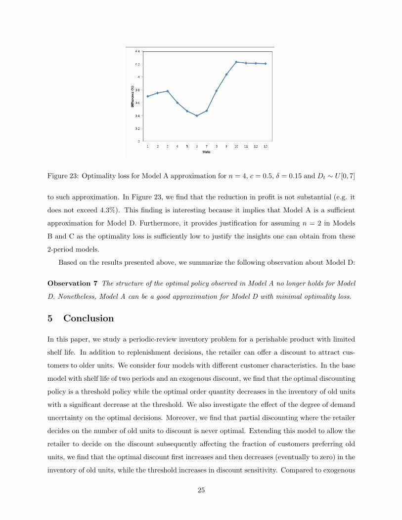
Figure 23: Optimality loss for Model A approximation for n = 4, c = 0.5, δ = 0.15 and Dt ∼ U [0, 7]
to such approximation. In Figure 23, we find that the reduction in profit is not substantial (e.g. it
does not exceed 4.3%). This finding is interesting because it implies that Model A is a sufficient
approximation for Model D. Furthermore, it provides justification for assuming n = 2 in Models
B and C as the optimality loss is sufficiently low to justify the insights one can obtain from these
2-period models.
Based on the results presented above, we summarize the following observation about Model D:
Observation 7 The structure of the optimal policy observed in Model A no longer holds for Model
D. Nonetheless, Model A can be a good approximation for Model D with minimal optimality loss.
5 Conclusion
In this paper, we study a periodic-review inventory problem for a perishable product with limited
shelf life. In addition to replenishment decisions, the retailer can offer a discount to attract cus-
tomers to older units. We consider four models with different customer characteristics. In the base
model with shelf life of two periods and an exogenous discount, we find that the optimal discounting
policy is a threshold policy while the optimal order quantity decreases in the inventory of old units
with a significant decrease at the threshold. We also investigate the effect of the degree of demand
uncertainty on the optimal decisions. Moreover, we find that partial discounting where the retailer
decides on the number of old units to discount is never optimal. Extending this model to allow the
retailer to decide on the discount subsequently affecting the fraction of customers preferring old
units, we find that the optimal discount first increases and then decreases (eventually to zero) in the
inventory of old units, while the threshold increases in discount sensitivity. Compared to exogenous
25

discount, the increase in profits in generally not significant and the threshold is higher. Extending
the model further to allow a new pool of customers to be attracted solely to the old units, we
also consider the effect of two new parameters; namely, advertising effectiveness and the fraction
of bargain hunters (new customers who beat the original customers to the old products). In this
setting, the optimal order quantity increases in the inventory of old units due to the presence of new
customers. As advertising effectiveness increases, optimal order quantity and profit increases while
the optimal discount can be non-monotone. As fraction of bargain hunters increases, optimal order
quantity increases in a convex fashion, the optimal profit also increases while the optimal discount
behaves in certain patterns according to whether the inventory of old units is low or high. Finally,
extending the base model to shelf life longer than two periods, we observe that the structure of the
optimal policy no longer holds. However, we find that the base model can be used to approximate
say a four-period problem with minimal optimality loss. This suggests that one can learn insights
from two-period models without too much reduction in profits. Nonetheless, the option to set the
discount and the presence of bargain hunters for products with shelf life longer than two periods
are also interesting to study and analytically challenging to characterize optimally. We leave this
issue to future research.
26

References
Avinadav, T., A. Herbon, U. Spiegel. 2013. Optimal inventory policy for a perishable item with
demand function sensitive to price and time. International Journal of Production Economics
144(2) 497–506.
Chen, T. -H. 2017. Optimizing pricing, replenishment and rework decision for imperfect and deteri-
orating items in a manufacturer-retailer channel. International Journal of Production Economics
183 539–550.
Chen, X., D. Smichi-Levi. 2004. Coordinating inventory control and pricing strategies with random
demand and fixed ordering cost: The infinite horizon case. Mathematics of Operations Research
29(3) 698–723.
Chew, E. P., C. Lee, R. Liu, K. S. Hong, A. Zhang. 2014. Optimal dynamic pricing and ordering
decisions for perishable products. International Journal of Production Economics 157 39–48.
Cohen, M. A. 2006. Joint pricing and ordering policy for exponentially decaying inventory with
known demand. Naval Research Logistics Quarterly 24(2) 257–268.
Deniz, B., I. Karaesmen, A. Scheller-Wolf. 2010. Managing perishables with substitution: inventory
issuance and replenishment heuristics. Manufacturing and Service Operations Management 12(2)
319–329.
Ellickson, P. B., S. Misra. 2008. Supermarket pricing strategies. Marketing Science 27(5) 811–828.
Elmaghraby, W., P. Keskinocak. 2003. Dynamic Pricing in the presence of inventory considerations:
Research overview, current practices, and future directions. Management Science 49(10) 1287–
1309.
Federgruen, A., A. Heching. 1999. Combined pricing and inventory control under uncertainty.
Feng, L., Y. -L. Chan, L. E. Cardenas-Barron. 2017. Pricing and lot-sizing polices for perish-
able goods when the demand depends on selling price, displayed stocks, and expiration date.
International Journal of Production Economics 185 11–20.
Ferguson, M. E., Oded Koenigsberg. 2007. How should a firm manage deteriorating inventory?
Production and Operations Management 16(3) 306–321.
27

Haijema, R. 2014. Optimal ordering, issuance and disposal policies for inventory management of
perishable products. International Journal of Production Economics 157 158–169.
Herbon, A., E. Levner, T. C. E. Cheng. 2014. Perishable inventory management with dynamic
pricing using time-temperature indicators linked to automatic detecting devices. International
Journal of Production Economics 147 605–613.
Hopp, W. J., X. Xu. 2006. A monopolistic and oligopolistic stochastic flow revenue management
model. Operations Research 54(6) 1098–1109.
Kapner, S. 2013. Penney sales yet to pick up after Johnson exit.
Http://www.wsj.com/articles/SB10001424127887324767004578487461030277932.
Lal, R., R. Rao. 1997. Supermarket competition: The case of Everyday Low Pricing. Marketing
Science 16(1) 60–80.
Li, Y., B. Cheang, A. Lim. 2012. Grocery perishables management. Production and Operations
Management 21(3) 504–517.
Li, Y., A. Lim, B. Rodrigues. 2009. Pricing and inventory control for a perishable product. Man-
ufacturing and Service Operations Management 11(3) 538–542.
Mourdoukoutas, P. 2013. A strategic mistake that haunts JC Penney.
Http://www.forbes.com/sites/panosmourdoukoutas/2013/09/27/a-strategic-mistake-that-
haunts-j-c-penney/.
Nahmias, S. 1975. Optimal ordering policies for perishable inventory-II. Operations Research 23(4)
735–749.
Nahmias, S. 1982. Perishable inventory theory: A review. Operations Research 30(4) 680–708.
Nahmias, S. 2011. Perishable Inventory Systems. Springer.
Pauls-Worm, K. G. J., E. M. T. Hendrix, A. J. Alcoba, R. Haijema. 2016. Order quantities for
perishable inventory control with non-stationary demand and a fill rate constraint. International
Journal of Production Economics 181 238–246.
Petruzzi, N.C., M. Dada. 1999. Pricing and the newsvendor problem: A review with extensions.
Operations Research 47(2) 183–194.
28
Pierskalla, W. P. 1969. An inventory problem with obsolescence. Naval Research Logistics Quarterly
16 217–228.
Pierskalla, W. P., C. D. Roach. 1972. Optimal issuing policies for perishable inventory. Management
Science 18(11) 603–614.
Rajan, A., R. Steinberg, R. Steinberg. 1992. Dynamic pricing and ordering decisions by a monop-
olist. Management Science 38(2) 240–262.
Sainathan, A. 2013. Pricing and replenishment of competing perishable product variants under
dynamic demand substitution. POMS 22(5) 1157–1181.
Thau, B. 2013. Another reason J.C. Penney’s ‘No Sale’ strategy flopped: Digital deals are prolif-
erating. Http://www.forbes.com/sites/barbarathau/2013/05/08/another-reason-j-c-penneys-no-
sale-strategy-flopped-digital-deals-are-proliferating/.
Thowsen, G.T. 1975. A dynamic, nonstationary inventory problem for a price/quantity setting
firm. Naval Research Logistics Quarterly 22 461–476.
van Donselaar, K. H., J. Peters, A. de Jong, R. A. C. M. Broekmeulen. 2016. Analysis and fore-
casting of demand during promotions for perishable items. International Journal of Production
Economics 172 65–75.
Zabel, E. 1970. Monopoly and uncertainty. The Review of Economic Studies 37(2) 205–219.
29