Special Issue on Power Electronics & Systems: Modeling, Analysis, Control, and Stability, 2017

Optimal Design of Controller Parameters for Improving the Stability of

MMC-HVDC for Wind Farm Integration

Jing Lyu1, Marta Molinas1, Xu Cai2

1. Department of Engineering Cybernetics, Norwegian University of Science and Technology, Trondheim 7491, Norway

2. Wind Power Research Center, Shanghai Jiao Tong University, Shanghai 200240, China

Abstract—A subsynchronous oscillation (SSO) phenomenon has been observed in a modular multilevel converter-based

high-voltage DC (MMC-HVDC) transmission system for wind farm integration in the real world, which is independent of

the type of wind turbine generator. This kind of oscillation appears different from those in DFIG-based wind farm with

series-compensation line or wind farm integration through two-level VSC-HVDC transmission system, because the internal

dynamics of the MMC may have significant impact on the oscillation. By far, however, very few papers have reported it.

In this paper, the generation mechanism of the SSO phenomenon in an MMC-HVDC transmission system for wind farm

integration is revealed from an impedance point of view. The harmonic state-space (HSS) modeling method is applied to

model the multi-frequency behavior of the MMC, based on which, the ac-side small-signal impedance of the MMC is

analytically derived according to harmonic linearization theory. As a general rule, the controller parameters of the wind

power inverter and the HVDC converter are designed separately, to meet the performance requirements of the single

converter under ideal conditions, but this practice does not guarantee the stability of the interconnected system. Therefore,

an optimal design method for controller parameters is proposed in this paper in order to guarantee the stability of the

interconnected system from a system point of view. Finally, time-domain simulations validate the effectiveness of the

theoretical analysis and the proposed optimal design method.

Index Terms—Modular multilevel converter (MMC), HVDC, wind farm, stability, controller parameter design.

Statement: This paper is original and has never been submitted to any other journals or conferences. Jing Lyu is the corresponding author for this work. Address: Department of Engineering Cybernetics, NTNU, Trondheim-7491, Norway Phone: +47 92297235, E-mail: jing.lyu@ntnu.no

I. INTRODUCTION

Modular multilevel converter-based high-voltage dc (MMC-HVDC) transmission technology is a promising solution for

integrating large-scale and long-distance offshore wind farms into onshore power grid, due to its high modularity, low switching

loss, low distortion of output voltage, decoupling control of active and reactive power, and so on [1], [2]. However, because of the

complex internal structure of MMC, the modeling and control of MMC is much more complex than that of two-level voltage-

source converters (VSCs) [3], [4]. Moreover, the internal dynamics of MMC such as capacitor voltage fluctuations and harmonic

circulating currents may have harmful effects on the stable operation of MMC-based interconnected systems, especially for

renewable energy integration applications [5], [6]. Fig. 1 demonstrates the on-site recorded waveforms of the wind farm side MMC

(WFMMC) in a certain MMC-HVDC project for wind farm integration in China [7], where the output power of the wind farm is

approximately 20% of the rated power. As can be seen, there is an obvious subsynchronous oscillation (SSO) phenomenon in the

ac- and dc-side currents, and the dominant oscillation frequency is approximately 20 Hz in the ac-side and 30 Hz in the dc-side.

When the output power of the wind farm further increased, the MMC-HVDC system was shut down by the protection system,

leading to the outage of the wind farm. Furthermore, it is worth noting that there are several different types of wind farms in the

project, including fixed speed induction generator (FSIG)-based wind farm, doubly-fed induction generator (DFIG)-based wind,

and permanent magnet synchronous generator (PMSG)-based wind farm, and a similar oscillation phenomenon appeared when

each type of wind farm was separately connected to the MMC-HVDC transmission system.

Fig. 1. On-site recorded waveforms in a real MMC-HVDC project for wind farm integration

So far, very few papers have discussed the stability of wind farms integrated with MMC-HVDC transmission systems. An SSO

phenomenon in an MMC-HVDC transmission system for wind farm integration was reported in [5], in which the distribution and

propagation mechanisms of the SSO currents in the MMC-HVDC system were investigated and an SSO current suppression

strategy was also proposed, but the mechanism by which these oscillations are generated in the MMC-HVDC system with wind

farms wasn’t deeply analyzed nor identified. The impedance-based analysis method was used to analyze the small-signal stability

of wind farm integration through MMC-HVDC in [6], [8], where the impacts of power transfer level, circulating current control,

and controller parameters on the stability of the interconnected system were discussed. However, neither controller parameter

design methods or stabilization control methods for enhancing the stability of the interconnected system were deeply discussed in

those above papers. In addition, voltage stability of offshore wind farms integrated with a VSC-HVDC transmission system was

studied by using impedance-based method in [9], in which, however, the VSC-HVDC system is based on two-level VSC that lacks

internal dynamics, so the instability mechanism might not be able to exactly explain the SSO phenomenon in the MMC-HVDC

connected wind farms.

The eigenvalue-based analysis method is commonly used to investigate the small-signal stability of MMC-based power systems

[10]-[15]. However, most of the authors have overlooked the internal dynamics of MMC in the course of developing small-signal

models, which leads to the small-signal model analogous to that of the two-level VSC. Besides, a few authors have built the small-

signal model of MMC in the rotating dq frames at different frequencies so as to have the internal dynamics of MMC been

considered [13]-[15], and then the impact of the internal dynamics on MMC stability was analyzed using eigenvalue analysis. In

addition, nonlinear analysis methods such as Lyapunov [16], [17] and Floquet [18] theory have also been introduced to analyze

the MMC stability, which, however, have some important disadvantages, such as complexity of analysis, difficulty in application,

inconvenience for guiding control system design, etc.

This paper focuses on the small-signal stability of MMC-HVDC connected wind farms by using impedance-based analysis

method. In order to obtain an accurate MMC model, the harmonic state-space (HSS) modeling method [19], which is based on the

linear time periodic (LTP) theory and is able to include all the harmonic dynamics, is introduced to model the MMC in this work.

On the basis of the HSS model, the ac-side small-signal impedance of MMC is then derived according to the harmonic linearization

principle [20]. The derived MMC impedance model in this paper is able to include the effects of all the internal harmonics on the

impedance response. Next, the generation mechanism of the SSO phenomenon in the MMC-HVDC connected wind farm is

revealed based on the terminal impedance characteristics. On the basis of the instability mechanism analysis, an optimized design

method on the ac voltage controller of WFMMC is proposed from a systemic perspective in order to guarantee the stability of the

interconnected system. Finally, time-domain simulations are carried out in MATLAB/Simulink to validate the effectiveness of the

theoretical analysis and the proposed optimization design method.

The rest of the paper is organized as follows. Section II describes the configuration and control of the system under study.

Section III presents the HSS modeling of MMC, and the impedance modeling and verification for MMC are elaborated in Section

IV. The instability mechanism is first revealed, and on this basis, the optimized design method for the ac voltage controller of

WFMMC are then proposed in Section V. Time-domain simulations are carried out in Section VI. Section VII concludes the paper.

II. CONFIGURATION AND CONTROL OF THE INTERCONNECTED SYSTEM

A. System Configuration under study

Fig. 2 shows the structure diagram of wind farm integration through an MMC-HVDC transmission system. Fig. 2(a)

demonstrates the overall structure of the system, where the wind farm consists of full-power wind turbines based on two-level

VSCs, and the MMC-HVDC transmission system comprises a WFMMC, a grid side MMC station (GSMMC), and dc transmission

lines. In addition, T1 and T2 are the converter transformers, and T3 is the step-up transformer of the wind farm. Fig. 2(b) presents

the MMC topology used for both WFMMC and GSMMC. Each phase-leg of the MMC consists of one upper and one lower arm

connected in series between the dc terminals. Each arm consists of N identical series-connected submodules (SMs), one arm

inductor L, and an arm equivalent series resistor R. Each SM contains a half-bridge as a switching element and a dc storage

capacitor CSM.

(a)

(b)

Fig. 2. Structure diagram of wind farm integration through an MMC-HVDC transmission system. (a) Overall structure. (b) MMC topology.

For simplification of analysis, the wind farm is modeled by an aggregated full-power wind turbine. Furthermore, since the grid

side converter of the wind turbine is decoupled with the generator side converter by the dc link capacitor, the generator side

dynamics have less impact on the grid side dynamics, so the turbine mechanical and generator side converter can be replaced with

a constant power source [9]. In addition, it is assumed that the ac power grid is strong and the control bandwidth of the dc voltage

loop of the GSMMC is less than the SSO frequency under study (i.e. 20 Hz in this paper), which means the dc voltage control

dynamics of the GSMMC have little effect on the ac-side dynamics of the WFMMC. Consequently, the GSMMC can be simply

replaced with a dc voltage source. The simplified circuit structure diagram of the interconnected system is presented in Fig. 3,

where T4 is the step-up transformer of the wind turbine, and Lw is the ac filter inductance of the wind turbine.

Fig. 3. Simplified circuit structure of the interconnected system.

B. System Control

Since the WFMMC has to supply an ac voltage source for the wind farm, a single-loop ac voltage control in the three-phase

stationary abc frame is employed in the WFMMC, as shown in Fig. 4, where Hv(s) is an ac voltage regulator, a proportional-

resonant (PR) regulator is used to achieve the zero steady-state error for the sinusoidal quantities; kf is a feed-forward gain for

improving the dynamic response of the control system. The nearest level modulation (NLM) [21] and sorting-based capacitor

voltage balancing control [22] are used in the MMC.

The transfer function of the ac voltage regulator is

( ) ( )2 21

pvv pv

iv

K sH s K

T s ω= +

+ (1)

where Kpv and Tiv are the proportional gain and integral time constant of the PR regulator, respectively; ω1 is the fundamental

angular frequency.

The conventional current vector control strategy in a rotating dq frame with feedforward and decoupling terms is used for the

wind power inverter, as presented in Fig. 5, where a PLL ensures that the d-axis of the rotating dq frame is aligned with the grid

voltage vector. Fig. 5(a) shows the current control, where *wdi is the active current reference which is given as a constant value

according to the active power command, *wqi is the reactive current reference which is set as zero in this paper, and Hi(s) is a current

regulator based on a proportional-integral (PI) regulator, which is given by

( ) 11i piii

H s KT s

= +

(2)

where Kpi and Tii are the proportional gain and integral time constant of the current PI regulator, respectively.

Fig. 5(b) shows the PLL diagram, where HPLL(s) is a PI regulator, which is given by

( ) 11PLL ppip

H s KT s

= +

(3)

where Kpp and Tip are the proportional gain and integral time constant of the PLL regulator, respectively.

Fig. 4. Control diagram of WFMMC.

(a) (b)

Fig. 5. Control diagram of wind power inverter. (a) Current control. (b) PLL.

III. HARMONIC STATE SPACE (HSS) MODELING OF MMC

A. Formulation of Harmonic State Space Modeling

For any time-varying periodic signal x(t), it can be written in the form of Fourier series as:

( ) 1jk tk

kx t X e ω

∈

= ∑

(4)

where ω1=2π/T, T is the fundamental period of the signal, and Xk is the Fourier coefficient that can be calculated by

( )01

0

1 t T jk tk t

X x t e dtT

ω+ −= ∫ (5)

The state-space equation of an LTP system can be expressed as

( ) ( ) ( ) ( ) ( )x t A t x t B t u t= + (6)

Based on the Fourier series and harmonic balance theory, the state-space equation in time-domain can be transformed into the

harmonic state-space equation in frequency-domain, which is like

( )s = − +X A N X BU (7)

where X, U, A, B, and N are indicated as (8)~(12), respectively, of which the elements Xh, Uh, Ah, and Bh are the Fourier coefficients

of the hth harmonic of x(t), u(t), A(t), and B(t) in (6), respectively. Note that A and B are Toeplitz matrices in order to perform the

frequency-domain convolution operation, N is a diagonal matrix that represents the frequency information, and I is an identity

matrix. In addition, it should be noted that the harmonic order h considered in the model needs to be selected according to the

requirements for accuracy and complexity of the model.

[ ]1 0 1, , , , , , Th hX X X X X− −=X (8)

[ ]1 0 1, , , , , , Th hU U U U U− −=U (9)

0 1

1

0 1

1 0 1

1 0

1

1 0

h

h h

h

A A AA

A AA A A A A

A AA

A A A

− −

−

− −

−

=

A

(10)

0 1

1

0 1

1 0 1

1 0

1

1 0

h

h h

h

B B BB

B BB B B B B

B BB

B B B

− −

−

− −

−

=

B

(11)

1

1

0

jh I

I

jh I

ω

ω

− =

N

(12)

B. HSS Modeling of MMC

Fig. 6 presents the average-value model of one phase leg of MMC, where Carm=CSM/N, CSM is the submodule capacitance, L and

R are the arm inductance and equivalent series resistance, iu and il are the upper and lower arm currents, cuv∑ and clv∑ are the sum

capacitor voltages of the upper and lower arms, vg and ig are the ac-side phase voltage and current, ic is the circulating current, Vdc

is the dc bus voltage, and nu and nl are the switching functions of the upper and lower arms. In addition, ZL is the equivalent load

impedance on the ac-side of MMC, and vp is the injected small perturbation voltage in order to develop the small-signal impedance

of MMC according to the harmonic linearization theory. Furthermore, the dc-link voltage Vdc is assumed to be constant.

Fig. 6. Average-value model of one phase leg of MMC.

According to Fig. 6, the time-domain state-space equation of one phase leg of MMC can be expressed as equation (6), where

x(t), u(t), A(t), and B(t) are indicated as follows:

( )T

c cu cl gx t i v v i∑ ∑ = (13)

( ) [ ]dcu t V= (14)

( )

02 2

0 02

0 02

20

u l

u u

arm arm

l l

arm arm

u l L

n nRL L L

n nC C

A tn n

C Cn n R ZL L L

− − − = − +

− −

(15)

( ) 1 0 0 02

T

B tL

= (16)

where the switching functions nu and nl are determined by the controller employed in the MMC, which can be expressed as

( )

( )

1 1

1 1

1 1 cos21 1 cos2

u m

l m

n m t

n m t

ω θ

ω θ

= − + = + +

(17)

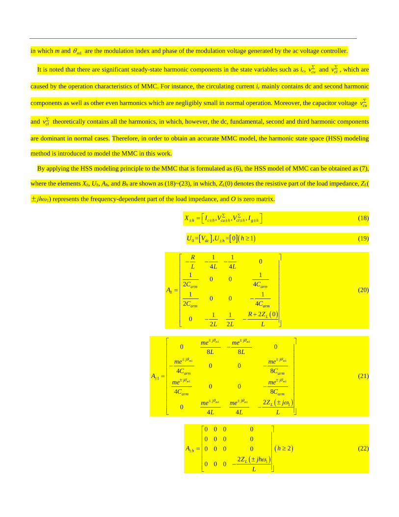
in which m and 1mθ are the modulation index and phase of the modulation voltage generated by the ac voltage controller.

It is noted that there are significant steady-state harmonic components in the state variables such as ic, cuv∑ and clv∑ , which are

caused by the operation characteristics of MMC. For instance, the circulating current ic mainly contains dc and second harmonic

components as well as other even harmonics which are negligibly small in normal operation. Moreover, the capacitor voltage cuv∑

and clv∑ theoretically contains all the harmonics, in which, however, the dc, fundamental, second and third harmonic components

are dominant in normal cases. Therefore, in order to obtain an accurate MMC model, the harmonic state space (HSS) modeling

method is introduced to model the MMC in this work.

By applying the HSS modeling principle to the MMC that is formulated as (6), the HSS model of MMC can be obtained as (7),

where the elements Xh, Uh, Ah, and Bh are shown as (18)~(23), in which, ZL(0) denotes the resistive part of the load impedance, ZL(

±jhω1) represents the frequency-dependent part of the load impedance, and O is zero matrix.

, , ,h c h cu h cl h g hX I V V I∑ ∑± ± ± ± ± = (18)

[ ] [ ]( )0 = , = 0 1dc hU V U h± ≥ (19)

( )

0

1 1 04 4

1 10 02 4

1 10 02 4

2 01 102 2

arm arm

arm arm

L

RL L L

C CA

C CR Z

L L L

− − − = − +

− −

(20)

( )

1 1

1 1

1 1

1 1

1

1

0 08 8

0 04 8

0 04 8

20

4 4

m m

m m

m m

m m

j j

j j

arm armj j

arm armj j

L

me meL L

me meC C

Ame me

C CZ jme me

L L L

θ θ

θ θ

θ θ

θ θ ω

± ±

± ±

± ± ±

± ±

−

− −

= −

± −

(21)

( )( )

1

0 0 0 00 0 0 0

20 0 0 02

0 0 0

h

L

A h

Z jhL

ω±

= ≥

± −

(22)

( )4 10

1 0 0 0 , 12

T

hB B O hL

×±

= = ≥ (23)

The harmonic state-space model, in which harmonics of state variables, inputs and outputs are posed separately in a state-space

form, can be used for dynamic small-signal studies and for harmonic steady-state studies [19]. Letting the left side of (7) to be zero,

the steady-state harmonic components of state variables can thus be calculated by

( ) 1ss

−= − −X A N BU (24)

Fig. 7 shows a comparison between the steady-state results of the HSS model and the nonlinear time-domain simulation model

in MATLAB/Simulink, where the harmonic order h=3 in the HSS model of MMC, and the MMC parameters are listed in Appendix

Table I. It can be seen that the results between the HSS model and the simulation model have a good match, which indicates that

the HSS model of MMC developed in this paper is able to capture all the steady-state harmonics in the circulating current and

capacitor voltage, and is accurate enough for harmonic steady-state studies. In addition, it should be noted that the results from the

HSS model can be converted into the time-domain signals by using (4).

(a) (b)

Fig. 7. Validation for the HSS model of MMC. (a) Circulating current ic. (b) Capacitor voltage cuv∑ .

IV. IMPEDANCE MODELING AND VERIFICATION

The impedance modeling of the interconnected system as shown in Fig. 3 includes two parts, i.e., the WFMMC impedance

ZWFMMC and the wind farm impedance Zwf. The wind farm impedance mainly includes the aggregated wind turbine, transformers

and equivalent lines, in which, the key issue is the impedance modeling of wind turbine. Since the wind turbine is based on two-

level VSCs and the impedance modeling of two-level VSCs has been well studied [23], [24], the detailed impedance derivations

of the wind farm will be no longer presented in this paper. This section will focus on the impedance modeling of MMC.

1 1.01 1.02 1.03 1.04 1.050

20

40

60

80

100

120

Time (s)

Circ

ulat

ing

curre

nt (A

)

HSS modelSimulation model

1 1.02 1.04 1.06 1.08 1.12.9

3

3.1

3.2

3.3

3.4

3.5x 10

5

Time (s)

Cap

acito

r vol

tage

(V)

HSS modelSimulation model

A. Impedance Modeling of MMC

According to the harmonic linearization principle [20], by injecting a small sinusoidal perturbation voltage in the ac-side of

MMC (as shown in Fig. 6) and then calculating the corresponding current response of the MMC at the perturbation frequency, the

ac-side small-signal impedance can thus be obtained by calculating the ratio of the resulting complex voltage to current at the

perturbation frequency, which is defined as

( ) gpMMC p

gpZ jω = −

vi

(25)

where the bold letters vgp and igp represent the complex phasors of small perturbations vgp(t) and igp(t) at frequency ωp, respectively.

According to the operation principle of MMC, the perturbation component at frequency ωp of the arm current will produce the

perturbation components at frequency (ωp±ω1) in the capacitor current by interacting with the fundamental modulation function.

These perturbation components in the capacitor current will lead to the corresponding perturbation components in the capacitor

voltage, which will in turn generate the perturbation components at frequency (ωp±2ω1) in the arm current by interacting with the

fundamental modulation function. Therefore, in turn, the following perturbation components at frequency ωp±3ω1, ωp±4ω1… can

then be created. Consequently, the injected small perturbation voltage will lead to perturbations in all variables at frequencies that

are listed as follows:

1 1 1, , 2 , ,p p p p hω ω ω ω ω ω ω± ± ± (26)

The small perturbation equation of the MMC can be expressed as

( ) ( ) ( ) ( ) ( )p p p p px t A t x t B t u t= + (27)

where

( )T

p cp cup clp gpx t i v v i∑ ∑ = (28)

( ) , ,T

p up lp pu t n n v = (29)

( )

02 2

0 02

0 02

20

us ls

us us

arm armp

ls ls

arm arm

us ls L

n nRL L L

n nC C

A tn n

C Cn n R ZL L L

− − − = − +

− −

(30)

( )

02 2

1 0 02

10 02

2

cus cls

gscs

armp

gscs

arm

cus cls

v vL L

ii

CB t

ii

C

v vL L L

∑ ∑

∑ ∑

− −

+ = −

− −

(31)

where the subscript “s” and “p” denote steady-state and perturbation components, respectively. In addition, the small perturbations

nup and nlp of the switching functions are determined by the used controller (the ac voltage controller as shown in Fig. 4 is used in

this paper), which can be obtained as

f vup gp v gp

dc

f vlp gp v gp

dc

k HG

Vk H

GV

−= − −

− =

n v v

n v v (32)

where the bold letters denote complex phasors, e.g., vgp is vpjgpV e ϕ . Additionally, the small perturbation vgp can be expressed as

gp p L gpZ= +v v i (33)

By combining (26)~(33), the small perturbation HSS equation of the MMC can be obtained as

( )p p p p p ps = − +X A N X B U (34)

where Xp, Up, and Np, are given as (35)~(37), the elements of Ap and Bp are shown in (38)~(44), in which the subscript “p±h”

denotes the perturbation component at frequency “ 1p hω ω± ”, the subscript “0”, “±1”, and “±2” represent the Fourier coefficient

values of the state variables at frequency dc, ±ω1, and ±2ω1, respectively, which can be calculated by (24). Furthermore, the steady-

state harmonics above third-order are usually negligibly small.

, , , ,

, , ,

Tp p h p p h

p h cp h cup h clp h gp h

X X X

X I V V I

− +

∑ ∑± ± ± ± ±

= =

X

(35)

[ ]( )

, , , ,

, = 0 1

Tp p h p p h

p p p h

U U U

U V U h

− +

±

= = ≥

U

(36)

( )

( )

4 41

4 4

4 41

p

p p

p

j h I

j I

j h I

ω ω

ω

ω ω

×

×

×

−

= +

N

(37)

( ) ( )

( )

( )

( ) ( )

0 0

00

00

0

0 0

1 14 4 2

21 10 02 4

21 10 02 4

21 102 2

v cu clL p

gv c

L parm arm arm

gv c

L parm arm arm

v cu clL p

G V VR Z jL L L L

IG I

Z jC C C

AI

G IZ j

C C C

G V VR Z jL L L L

ω

ω

ω

ω

∑ ∑

∑ ∑

− − − − + − = − − + + − − − +

(38)

( ) ( )

( )

( )

1 1

1 1

1 1

1 1

1 11

11

1

11

1

1

1

08 8 2

20 0

4 8

20 0

4 8

04 4

m m

m m

m m

m m

j j v cu clL p

gv cj j

L parm arm arm

gv cj j

L parm arm arm

j j v cu cl

G V Vme me Z j jL L L

IG I

me me Z j jC C C

AI

G Ime me Z j j

C C C

G V Vme meL L

θ θ

θ θ

θ θ

θ θ

ω ω

ω ω

ω ω

∑ ∑± ±± ±

±±± ±

±±

±± ±

∑± ±±

−− ±

+

− − − ±

=

− − + ±

+( ) ( )11

2L pZ j j

Lω ω

∑±

− ±

(39)

( ) ( )

( )

( )

( ) ( )

2 21

22

1

22

2

1

2 21

0 0 0 22

20 0 0 2

20 0 0 2

20 0 0 2

v cu clL p

gv c

L parm

gv c

L parm

v cu clL p

G V VZ j j

LI

G IZ j j

CA

IG I

Z j jC

G V VZ j j

L

ω ω

ω ω

ω ω

ω ω

∑ ∑± ±

±±

±±

±

∑ ∑± ±

− ± + − ± = − ± + − ±

(40)

( )( )

1

0 0 0 00 0 0 00 0 0 0 3

20 0 0

h

L p

A h

Z j jh

L

ω ω±

= ≥

− ±

(41)

( ) ( )0 0

0 00 0 0 0

0

22 2, , ,

2

Tg g

v c v cv cu cl v cu cl

arm arm

I IG I G IG V V G V V

BL C C L

∑ ∑ ∑ ∑

+ − − + − = −

(42)

( ) ( )( )

2 2, , , 1, 2

2

Tg h g h

v c h v c hv cu h cl h v cu h cl h

harm arm

I IG I G IG V V G V V

B hL C C L

± ±∑ ∑ ∑ ∑± ±

± ± ± ±±

+ − − + = − =

(43)

( )4 4 3hB O h×± = ≥ (44)

By ignoring the transient behavior of the perturbation signals, that is, letting the left-hand side of (34) to be zero, the perturbation

components of the state variables at each perturbation frequency in (26) can thus be calculated by

( ) 1p p p p p

−= − −X A N B U (45)

According to the definition of small-signal impedance in (25), only the resulting perturbation voltage and current at frequency

ωp in the ac-side of MMC need to be considered. From (45), the perturbation current igp at frequency ωp can be calculated. In order

to solve (45), the harmonic order h must be determined first. After calculating the perturbation current igp, the perturbation voltage

vgp can be readily obtained by (33). Finally, the ac-side small-signal impedance of MMC at frequency ωp can thus be calculated by

(25). With different frequencies ωp, the impedance frequency characteristics of MMC can be obtained. In addition, it should be

noted that different values of h will generate different impedance expressions which means impedance models with different

accuracies. The ac-side impedance responses of MMC with different values of h will be presented and discussed in the next

subsection. Taking h=1 for example, the analytical impedance expression of MMC with open loop control is given in Appendix

(B1). It needs to be pointed out that the analytical impedance expression of the MMC with consideration of high harmonic order h

will become much more complex. However, with the help of computer, the complex impedance calculation as well as the

impedance-based stability analysis can be readily manipulated.

B. Impedance Model Verification

To verify the derived impedance model of the MMC, a nonlinear time-domain simulation model of a three-phase MMC with a

three-phase resistor load has been built by using MATLAB/Simulink. In the simulation, the ac-side small-signal impedance of the

MMC is measured by means of injecting a series of small perturbation voltage signals at different frequencies in the ac-side of the

MMC. Then by measuring the resulting perturbation current signals, the ac-side small-signal impedance can be readily calculated

for each frequency. The simulation parameters are listed in Appendix Table I.

Fig. 8 presents the comparison between the analytical and simulation measured ac-side small-signal impedances of the MMC,

where the harmonic order h of the analytical model is selected as 4. As can be seen, the analytical impedance matches well with

the simulation measured result, which validates the effectiveness of the analytical impedance model of the MMC.

Fig. 9 shows the impact of the harmonic order selected in the HSS model of MMC on the analytical impedance response. It can

be observed that the harmonic order selected in the HSS model of MMC has great impact on the accuracy of the analytical

impedance model. The higher the harmonic order selected in the HSS model is, the more accurate the analytical impedance model

is. However, in general case, only several significant low-order harmonics play dominant roles in the MMC impedance response,

due to the much smaller amplitude of the high-order harmonics. Generally, it can be concluded that the analytical impedance model

is accurate enough if the harmonic order h≥3.

Fig. 10 shows the comparison between the analytical impedance responses of the MMC with and without consideration of the

internal dynamics, where h=0 means that the MMC internal dynamics are not considered in the modeling. As can be seen, the

analytical impedance model without consideration of the MMC internal dynamics cannot reflect the low-frequency resonances,

which will result in definitely wrong results for low-frequency stability analysis in the MMC-HVDC connected wind farm.

Therefore, it is essential to consider the internal dynamics in the MMC modeling in order to accurately reveal the generation

mechanism of the subsynchronous oscillation in the interconnected system.

Fig. 8. Impedance model verification for the MMC.

Fig. 9. Impact of the harmonic order selected in the HSS model of MMC on the analytical impedance response.

Fig. 10. Comparison between the analytical impedance responses of the MMC with and without consideration of the internal dynamics.

V. INSTABILITY MECHANISM AND OPTIMAL CONTROLLER PARAMETER DESIGN

A. Instability Mechanism Analysis

According to the impedance-based stability criterion [25], if the wind farm and WFMMC are stable separately, the stability of

the interconnected system is determined by the ratio of the WFMMC impedance to the wind farm impedance, which is given by

( ) ( )( )

WFMMCm

wf

Z sT s

Z s= (46)

Fig. 11 shows the ac-side impedance-frequency characteristics of the WFMMC and wind farm under different power level

conditions, i.e. 10%, 20%, and 40% of the rated power, where no circulating current control is used in the WFMMC and wind

turbine operates at unity power factor. It is seen that the magnitude of the wind farm impedance decreases as the output active

power of the wind farm increases, while the phase of the wind farm is almost unchanged. Furthermore, the WFMMC impedance

is unrelated to the wind farm output power level. It is worth noting that the magnitude- frequency characteristics of the WFMMC

impedance and wind farm impedance can intersect around the low-frequency resonance peak of the WFMMC impedance where

the corresponding phase margin (PM) of the interconnected system becomes small or even less than zero as the output power of

the wind farm becomes large, e.g., 20% power level with phase margin of about 20°, and 40% power level with phase margin of

about 7° which indicates that the interconnected system is marginally stable and prone to oscillations at the frequency around the

magnitude peak point. That’s the key reason why the SSO phenomenon can happen in an MMC-HVDC system for wind farm

integration. However, it should be pointed out that the intersection doesn’t always arise, depending on many factors such as the

wind farm output power, control strategies and controller parameters of both the wind power inverter and WFMMC, etc.

100

102

104

-200

-100

0

100

200

Frequency (Hz)101 102100

Zwf ZWFMMC

10% 20% 40%Mag

nitu

de (Ω

)Ph

ase

(deg

)

Resonance points

Phase difference is 160°Phase difference is 173°

Fig. 11. AC-side impedance-frequency characteristics of the WFMMC and wind farm.

B. Controller Parameter Design for Single Converter

In general, the controller parameters of the wind power inverter and WFMMC are tuned independently, to meet the performance

requirements of the single converter under ideal conditions. This practice however does not guarantee the stability of the

interconnected system. Nevertheless, the controller parameter design of each single converter is a precondition, based on which,

in this paper, the controller parameters are further optimized in order to guarantee the stability of the interconnected system from

a system perspective. As mentioned above, there are mainly three kinds of controllers in the interconnected system, i.e. the ac

voltage controller of WFMMC, the current controller and PLL controller of the wind power inverter, where the parameter designs

of the latter two have been discussed in [26], [27], respectively. This paper will focus on the parameter design for the ac voltage

controller of WFMMC.

The transfer function diagram of the ac voltage control loop of WFMMC is shown in Fig. 12, where V*(s) represents reference

input voltage, Hv(s) is the voltage regulator, dsTe− denotes the time delay of the digital control system, Vc(s) is the reference

modulation voltage, I(s) and V(s) are the input current and output voltage of WFMMC, respectively, and Zo(s) represents the

equivalent impedance of the arm inductor at the ac-side of WFMMC.

Fig. 12. Transfer function diagram of the ac voltage control loop of WFMMC.

It should be pointed out that, since a PR regulator in stationary abc frame is equivalent to a PI regulator in synchronous rotating

dq frame, the PR regulator parameters can be identical to those of the PI regulator [26], [28]. Therefore, a PI regulator is used for

the voltage regulator Hv(s) in Fig. 12 in order to calculate the ac voltage controller parameters, which is given by

( ) 11v pviv

H s KsT

= +

(47)

where Tiv is the integral time constant of the PI regulator.

From Fig. 12, the closed-loop transfer function of the ac voltage control loop can be obtained as

( )( )

( )1

1

d

d

sTpv iv

v sTiv pv iv

K T s es

T s K T s e

−

−

+Φ =

+ + (48)

According to the definition of the bandwidth of the closed-loop system, we have

( ) ( )( )

1 11 2

b d

b d

j Tpv b iv

v b j Tb iv pv b iv

K j T ej

j T K j T e

ω

ω

ωω

ω ω

−

−

+Φ = =

+ + (49)

Hence, one can obtain

( )22 1

pvb

iv pv

K

T Kω =

− − (50)

It is noted from (50) that the bandwidth of the ac voltage control loop depends on the controller parameters. Furthermore, letting

ωb > 0 leads to (51), which is the available value range of the proportional gain of the ac voltage controller.

0 2 1pvK< < + (51)

Fig. 13. Relationship between the bandwidth of the ac voltage loop and controller parameters.

Fig. 13 illustrates the relationship between the bandwidth of the ac voltage control loop and controller parameters. As can be

seen, the bandwidth of the ac voltage control loop increases as the proportional gain Kpv increases, and decreases as the integral

time constant Tiv increases. As a general rule, the bandwidth of the ac voltage loop has an upper limit value, and the integral time

constant Tiv is 2~5 fundamental periods. Thereby, the proportional gain Kpv can be determined by the given bandwidth and integral

time constant.

C. Controller Parameter Optimal Design for the Interconnected System

The objective of the optimal design for the controller parameter is to guarantee the stability of the interconnected system. As

aforementioned, the key reason for the instability of wind farm integrated with MMC-HVDC is that there exists an intersection

between the magnitude-frequency characteristics of the wind farm impedance and the WFMMC impedance. Therefore, a sufficient

condition can be made to guarantee the stability of the interconnected system, that is, the magnitude of the impedance ratio Tm(s)

is less than unity over the entire frequency range, i.e. 1mT < for all frequencies, which is also the optimization target of the

controller parameters of the interconnected system.

To meet the sufficient condition by only modifying the controller parameters, there are two ways: 1) optimizing the controller

parameters of WFMMC; 2) optimizing the controller parameters of wind power inverter. Both ways can improve the stability of

the interconnected system to guarantee the stability. However, considering the practical application, the former only needs to

modify the controller parameters of WFMMC, while the latter needs to modify a number of controller parameters of the wind

turbines controllers. Hence, this paper will focus on the former, yet the design procedure of the latter is analogous to that of the

former. In addition, it should be pointed out that, since the magnitude-frequency characteristic mT of the impedance ratio is

associated with the power transfer level, and the stability margin reduces as the power transfer level increases, the controller

parameter optimal design will be carried out at the rated power.

The value range of the proportional gain in (51) is determined by only the bandwidth of the ac voltage loop, which will be further

optimized to meet the sufficient condition for the stability of the interconnected system. For that, the impacts of controller

parameters of the ac voltage controller of WFMMC on the magnitude-frequency characteristic mT of the impedance ratio need

to be analyzed first, and meanwhile the other parameters remain unchanged. The main parameters of the interconnected system

are listed in Appendix Table I and II.

Fig. 14 demonstrates the impact of the ac voltage controller parameters of WFMMC on the magnitude-frequency characteristic

mT of the impedance ratio. It is seen from Fig. 14(a) that, the maximum value of mT is at the low-frequency resonant frequency

of the WFMMC impedance; the resonance peak of mT decreases monotonously as the proportional gain Kpv increases within a

certain range, and mT can be less than unity by only increasing the proportional gain Kpv. Therefore, the stability of the

interconnected system can be improved by optimizing the proportional gain of the ac voltage controller of WFMMC. However,

the integral time constant Tiv of the ac voltage controller of WFMMC has little impact on the magnitude-frequency characteristic

mT of the impedance ratio, as shown in Fig. 14(b), the resonance peak of mT is always larger than unity as Tiv varying, which

indicates that it is not possible to improve the stability of the interconnected system by modifying the integral time constant of the

ac voltage controller of WFMMC.

(a) (b)

Fig. 14. Impact of the ac voltage controller parameters of WFMMC on the magnitude-frequency characteristic of the impedance ratio. (a) Impact of Kpv. (b)

Impact of Tiv.

As the above analysis shows, it is capable to improve the stability of the interconnected system by optimizing the proportional

gain of the ac voltage controller of WFMMC. Fig. 15 shows the flowchart of the optimal design procedure for the proportional

gain of the ac voltage controller of WFMMC. Fig. 16 illustrates the optimal value range of the proportional gain of the ac voltage

controller of WFMMC, in which the abscissa is the proportional gain Kpv, the left ordinate is the resonance peak of mT , and the

right ordinate is the control bandwidth of the ac voltage loop. It is noted that there exist two values of Kpv to make the resonance

peak of mT to be 1 in this case, however, the smaller one is not available. Moreover, in theory, the larger the control bandwidth

of the ac voltage loop of WFMMC is, the more stable the interconnected system is. However, the control bandwidth of the ac

voltage loop is limited by the allowed maximum of the system bandwidth. It should be pointed out that the proposed optimal design

method in this paper is a sufficient condition for the stability of the interconnected system.

Fig. 17 shows the relationship between the phase margin of the interconnected system and the proportional gain of the ac voltage

controller of WFMMC. As can be seen, under the system parameters used in this paper, the phase margin of the interconnected

system becomes positive when the proportional gain of the ac voltage controller of WFMMC is larger than 0.97, which means that

the interconnected system is stable, otherwise, the phase margin of the interconnected system becomes negative, the interconnected

system is unstable. Furthermore, in designing the system, sufficient stability margins have to be guaranteed in order to avoid small-

signal oscillations due to weak damping. The minimum Kpmin of the optimal value range of the proportional gain Kpv determined

by Fig. 16 is 1.35, corresponding to the phase margin of approximately 25° seen from Fig. 17, which indicates the interconnected

system has enough damping by using the optimal controller parameters.

Furthermore, it is worth noting that there is a positive correlation between the proportional gain Kpv satisfying the stability

requirement and the ac voltage loop bandwidth, which implies that the proportional gain Kpv within the optimal value range can

simultaneously meet the requirements for both the stability and dynamic characteristic of the system.

Fig. 15. Flowchart of the optimal design procedure for the proportional gain of the ac voltage controller of WFMMC.

Fig. 16. Illustration for the optimal value range of the proportional gain of the ac voltage controller of WFMMC.

Fig. 17. Relationship between the phase margin of the interconnected system and the proportional gain of the ac voltage controller of WFMMC.

However, controller parameters usually have a limited value range, which maybe can limit the optimization effect. For instance,

the proportional gain of the ac voltage controller of WFMMC has an available value range as shown in (51), which means that the

optimal value range of the proportional gain must be located in this range. Furthermore, the lower limit value of the optimal value

range is determined by the impedance ratio magnitude at the resonance frequency which is associated with the main circuit

parameters of WFMMC. Therefore, it is necessary to investigate the relationship between the optimal value range and the main

circuit parameters of WFMMC, such as arm inductance and submodule capacitance.

Table III shows the impact of main circuit parameters of WFMMC on the optimization result, where the optimization result

refers to the lower limit value Kpmin of the optimal value range of the proportional gain Kpv. The optimization results are calculated

by letting the impedance ratio 1mT = under the various combinations of the arm inductance and submodule capacitance, where

the variation range of the arm inductance is from 0.16 pu to 0.23 pu, and the variation range of the submodule capacitance is

H=30~50 ms (H refers to the equivalent capacity discharging time constant which is usually used to represent the values of the

submodule capacitance). H is defined as

220

13 2 32 SM cSM dc

SMN N

N C V C VH C

S NS

× ×= = ∝ (52)

where SN denotes the rated capacity of MMC, and Vc0 is the average dc voltage of submodule capacitor.

Table III: Impact of main circuit parameters of WFMMC on the optimization result

H/ms L/pu 30 34 37 40 43 46 50

0.16 2.19 2.95 3.32 8.6 2.9 2.06 1.72 0.17 2.58 3.56 5 3.38 1.87 1.67 1.53 0.18 3.26 5.25 3.35 2.2 1.65 1.59 1.42 0.19 5 5.36 2.3 1.9 1.6 1.43 1.37 0.20 5.8 2.6 2.13 1.7 1.53 1.38 1.32 0.22 6.9 2.21 1.85 1.59 1.42 1.35 1.25 0.23 3.5 2.1 1.58 1.5 1.34 1.31 1.07

From (52), the submodule capacitance can be calculated as

23N

SMdc

NSC H

V= (53)

In Table III, the shaded area is invalid region, since the optimization results go out of range of the allowed proportional gain in

(51), which means that the interconnected system cannot be stabilized by optimizing the proportional gain Kpv. However, according

to the selection method of main circuit parameters for MMCs [29], H=40 ms is recommended. Additionally, the selection of the

arm inductance must avoid the circulating current resonance, and L=0.2 pu is usually recommended with the considerations of

security and economy. On the basis of the above selection, it is possible to stabilize the interconnected system by optimizing the

proportional gain Kpv. In addition, it can be concluded that the large submodule capacitance and/or arm inductance is conducive to

the stability of the interconnected system according to Table III.

VI. SIMULATION RESULTS

In order to validate the theoretical analysis and the proposed optimal design method, a time-domain simulation model of the

interconnected system as presented in Fig. 3 is built by using MATLAB/Simulink. The simulation parameters of the interconnected

system are listed in Appendix Table I and Table II, where the controller parameters are designed from a single converter point of

view. In addition, it needs to be pointed out that both the wind farm and WFMMC can work well separately using the controller

parameters in Appendix Table II even at the rated power.

Fig. 18 shows the simulated results of the interconnected system by using the controller parameters in Appendix Table II under

20% of the rated power condition, where Fig. 18(a) are the three-phase ac phase voltages and currents at the PCC of the

interconnected system, Fig. 18(b) is the FFT analysis of the phase voltage. It can be seen that the interconnected system is stable,

but with slight oscillations. The FFT analysis shows that the dominant oscillation frequency is around 22 Hz, which is consistent

with the theoretical analysis in the previous subsection.

Fig. 19 shows the simulated results at the rated power by using the controller parameters in Appendix Table II. It is seen that

there are significant oscillations in the ac voltages and currents, and the dominant oscillation frequencies are approximately 26 Hz,

which further confirms the instability mechanism analysis in this paper. The simulated results show that the controller parameters

designed based on a single converter cannot guarantee the stability of the interconnected system in the case of no additional

damping measures.

-100

-50

0

50

100

Time (s)1.3 1.32 1.34 1.36 1.38 1.4 1.42 1.44 1.46 1.48 1.5

-100

0

100

Volta

ge (k

V)C

urre

nt (A

)

(a)

Frequency (Hz)0 50 100 150 200

01020304050

Mag

nitu

de (%

)

22

(b)

Fig. 18. Simulated results without optimal controller parameters. (a) Three-phase ac phase voltages and currents at PCC of the interconnected system. (b)

Frequency analysis of the ac phase voltage.

(a)

Frequency (Hz)0 50 100 150 200

01020304050

Mag

nitu

de (%

)

26

(b)

Fig. 19. Simulated results without optimal controller parameters. (a) Three-phase ac phase voltages and currents at PCC of the interconnected system. (b)

Frequency analysis of the ac phase voltage.

According to the proposed optimal design method for controller parameters proposed in this paper, the optimal value of the

proportional gain Kpv of the ac voltage controller of WFMMC is selected as 1.6, corresponding to a phase margin of approximately

30°. By only modifying the proportional gain Kpv of the ac voltage controller of WFMMC from 0.8 to 1.6, the interconnected

system becomes stable even at the rated power, as shown in Fig. 20. It can be seen that the voltages and currents are sinusoidal

without any oscillatory components. Fig. 21 presents the dynamic waveforms during the step change of the active power with

optimal controller parameters, where the output active power from wind farm increases from 30 MW to 50 MW. As can be seen,

the dynamic waveforms are good, indicating that the interconnected system has sufficient damping.

(a)

(b)

Fig. 20. Simulated results with optimal controller parameters. (a) Three-phase ac phase voltages and currents at PCC of the interconnected system. (b) Frequency

analysis of the ac phase voltage.

Fig. 21. Dynamic waveforms during the step change of the active power with optimal controller parameters.

VII. CONCLUSION

An optimal design on the ac voltage controller of WFMMC has been investigated in this paper in order to guarantee the stability

of MMC-HVDC connected wind farms. The impedance-based analysis approach is used in this work. First, the harmonic state-

space (HSS) model of MMC is established, which shows to be accurate enough for harmonic steady-state studies. On this basis,

the ac-side small-signal impedance of MMC is then derived from small perturbation HSS model. The results show that the internal

dynamics of MMC have a great influence on the impedance response, especially in the low frequency range (<100 Hz), and the

derived impedance model is able to capture all the resonance characteristics. Next, the generation mechanism of the SSO in the

MMC-HVDC connected wind farms is revealed by using impedance-ratio frequency characteristics analysis. On the basis of the

instability mechanism analysis, an optimal design method for controller parameters is proposed in order to improve and guarantee

the stability of the interconnected system, from a system perspective. The coupling relationship between the optimization results

and the main circuit parameters of WFMMC is also expounded. The theoretical analysis shows that the stability of the

interconnected system can be effectively improved and guaranteed by only modifying the proportional gain of the ac voltage

controller of WFMMC. Is this also true if the operating point changes or other condition changes in the system? The simulation

results confirm the effectiveness of the theoretical analysis.

APPENDIX A

TABLE I. MAIN ELECTRICAL PARAMETERS OF THE INTERCONNECTED SYSTEM

Parameter Value

WFMMC

Rated power 50 MW

Rated frequency 50 Hz

Rated dc voltage 320 kV

Rated voltage at PCC 110 kV

Rated voltage at converter side 166 kV

Submodule number per arm 20

Arm inductance 360 mH

Submodule capacitance 140 µF

Wind power inverter

Rated power 50 MW

Rated terminal voltage 690 V

Rated dc voltage 1100 V

Filter inductance 5 µH

TABLE II. CONTROLLER PARAMETERS

Parameter Value WFMMC ac voltage controller Kpv 0.8

Tiv 50 ms

Wind power inverter current controller Kpi 0.015

Tii 3.2 ms

PLL controller Kpp 0.24 Tip 15 ms

APPENDIX B

( ) ( 3 3 4 2 3 3 2 4 3 3 6 3 2 4 3 2 2 3 3 2 51 1 1 1

3 2 2 2 3 2 4 3 3 2 3 3 3 2 2 2 2 2 2 2 2 41 1 1

2 2 4 2 2 4 2 2 2 2 21 1

2 4 3

1 13 34 4

1 3 1 14 4 4 2

MMC p p p p p p p

p p p p p p

p p p

Z j jC L j C L jC L C L R C L R C L R

j C LR j C LR C R C R j C L Nm j C L Nm

j C L N j C L N C LNRm C LNRm

ω ω ω ω ω ω ω ω ω ω ω

ω ω ω ω ω ω ω ω ω

ω ω ω ω ω

= − + + − + +

− + − + − −

+ + −

((

3 2 3 2 2 2 21

2 2 2 2 2 2 2 2 2 2 2 4 2 2 2 2 2 21 1 1

2 2 2 4 2 3 4 3 2 3 2 2 41

2 2 2 3 2 2 51

3 12 8

1 1 3 1 1 14 4 4 64 16 83 1 3 1 1 1 / 2

16 64 16 256 64 64

2

p

p p p

p p p p

p p

C LNR j C NR m

j C NR m j C NR j C NR j CLN m j CLN m j CLN

j CLN CN Rm CN R j N m j N m j N C C L

C L C L j

ω ω

ω ω ω ω ω ω

ω ω ω ω ω

ω ω ω

− − +

− + + − + +

+ + − + − −

+ + 2 2 2 2 4 2 2 2 2 2 3 2 2 2 31 1 1

2 3 2 2 2 2 2 2 2 21 1

1 12 28 8

1 1 1 1 1 1 12 2 8 8 2 32 16

p p p p p p

p p p p p p

C LR j C LR C R C R CLNm CLNm

CLN CLN j CNRm j CNRm j CNR N m N

ω ω ω ω ω ω ω ω ω

ω ω ω ω ω ω ω ω

− + − + − −

− − + + + +

(B1)

REFERENCES

[1] M. A. Perez, S. Bernet, J. Rodriguez, S. Kouro, and R. Lizana, “Circuit topologies, modeling, control schemes, and applications of modular multilevel

converter,” IEEE Trans. Power Electron., vol. 30, no. 1, pp. 4-17, Jan. 2015.

[2] S. Dehnath, J. Qin, B. Bahrani, M. Saeedifard, and P. Barbosa, “Operation, control, and applications of the modular multilevel converter: a review,” IEEE

Trans. Power Electron., vol. 30, no. 1, pp. 37-53, Jan. 2015.

[3] L. Harnefors, A. Antonopoulos, S. Norrga, L. Ängquist, and H.P. Nee, “Dynamic analysis of modular multilevel converters,” IEEE Trans. Ind. Electron., vol.

60, no. 7, pp. 2526-2537, Jul. 2013.

[4] K. Ilves, A. Antonopoulos, S. Norrga, and H.P. Nee, “Steady-state analysis of interaction between harmonic components of arm and line quantities of modular

multilevel converters,” IEEE Trans. Power Electron., vol. 27, no. 1, pp. 57-68, Jan. 2012.

[5] J. Lv, P. Dong, G. Shi, X. Cai, H. Rao, and J. Chen, “Subsynchronous oscillation of large DFIG-based wind farms integration through MMC-based HVDC,”

in Proc. IEEE Power System Tech. Conf., 2014, pp. 2401-2408.

[6] J. Lyu, X. Cai, and M. Molinas, “Frequency domain stability analysis of MMC-based HVdc for wind farm integration,” IEEE Journal of Emerging and

Selected Topics in Power Electronics, vol. 4, no. 1, pp. 141-151, Mar. 2016.

[7] J. Lü, P. Dong, G. Shi, X. Cai, and X. Li, “Subsynchronous oscillation and its mitigation of MMC-based HVDC with large doubly-fed induction generator-

based wind farm integration,” Proceedings of the CSEE, vol. 35, no. 19, pp. 4852-4860, Oct. 2015.

[8] J. Lyu and X. Cai, “Impact of controller parameters on stability of MMC-based HVDC systems for offshore wind farms,” in Proc. IET RPG Conf., 2015, pp.

1-6.

[9] H. Liu and J. Sun, “Voltage stability and control of offshore wind farms with ac collection and HVDC transmission,” IEEE Journal of Emerging and selected

topics in Power Electronics, vol. 2, no. 4, pp. 1181-1189, Dec. 2014.

[10] N. T. Trinh, M. Zeller, K. Wuerflinger, and I. Erlich, “Generic model of MMC-VSC-HVDC for interaction study with ac power system,” IEEE Trans. Power

Syst., vol. 31, no.1, pp. 27-34, Jan. 2016.

[11] H. Saad, J. Mahseredjian, S. Dennetiere, and S. Nguefeu, “Interactions studies of HVDC-MMC link embedded in an AC grid,” Electr. Power Syst. Res., vol.

138, pp. 202-209, Sept. 2016.

[12] G. Bergna, J. A. Suul, and S. D’Arco, “Small-signal state-space modeling of modular multilevel converters for system stability analysis,” in Proc. IEEE ECCE,

2015, pp. 5822-5829.

[13] A. Jamshidifar and D. Jovcic, “Small-signal dynamic DQ model of modular multilevel converter for system studies,” IEEE Trans. Power Del., vol. 31, no. 1,

pp. 191-199, Feb. 2016.

[14] T. Li, A. M. Gole, and C. Zhao, “Harmonic instability in MMC-HVDC converters resulting from internal dynamics,” IEEE Trans. Power Del., vol. 31, no. 4,

pp. 1738-1747, Aug. 2016.

[15] G. Bergna, J. A. Suul, and S. D’Arco, “State-space modelling of modular multilevel converters for constant variables in steady-state,” in Proc. IEEE COMPEL,

2016, pp. 1-9.

[16] A. Antonopoulos, L. Ängquist, L. Harnefors, K. Ilves, and H. P. Nee, “Global asymptotic stability of modular multilevel converters,” IEEE Trans. Ind.

Electron., vol. 61, no. 2, pp. 603-612, Feb. 2014.

[17] L. Harnefors, A. Antonopoulos, K. Ilves, and H. P. Nee, “Global asymptotic stability of current-controlled modular multilevel converters,” IEEE Trans. Power

Electron., vol. 30, no. 1, pp. 249-258, Jan. 2015.

[18] N. R. Chaudhuri, R. Oliveira, and A. Yazdani, “Stability analysis of vector-controlled modular multilevel converters in linear time-periodic framework,” IEEE

Trans. Power Electron., vol. 31, no. 7, pp. 5255-5269, Jul. 2016.

[19] G. N. Love and A. R. Wood, “Harmonic state space model of power electronics,” in Proc. Int. Conf. Harmonics Quality of Power, Wollongong, Australia,

2008, pp. 1-6.

[20] J. Sun, “Small-signal methods for ac distributed power systems-a review,” IEEE Trans. Power Electron., vol. 24, no. 11, pp. 2545-2554, Nov. 2009.

[21] Q. Tu and Z. Xu, “Impact of sampling frequency on harmonic distortion for modular multilevel ocnverter,” IEEE Trans. Power Del., vol. 26, no. 1, pp. 298-

306, Jan. 2011.

[22] A. Lesnicar and R. Marquardt, “An innovative modular multilevel converter topology suitable for a wide power range,” in Proc. IEEE Power Tech. Conf.,

2003, pp. 1-6.

[23] M. Cespedes and J. Sun, “Impedance modeling and analysis of grid-connected voltage-source converters,” IEEE Trans. Power Electron., vol. 29, no. 3, pp.

1254-1261, Mar. 2014.

[24] B. Wen, D. Boroyevich, R. Burgos, P. Mattavelli, and Z. Shen, “Analysis of D-Q small-signal impedance of grid-tied inverters,” IEEE Trans. Power Electron.,

vol. 31, no. 1, pp. 675-687, Jan. 2016.

[25] J. Sun, “Impedance-based stability criterion for grid- connected inverters,” IEEE Trans. Power Electron., vol. 26, no. 11, pp. 3075-3078, Nov. 2011.

[26] D. G. Holmes, T. A. Lipo, B. P. McGrath, W. Y. Kong, “Optimized design of stationary frame three phase ac current regulators,” IEEE Trans. Power Electron.,

vol. 24, no. 11, pp. 2417-2426, Nov. 2009.

[27] Y. Wang, X. Chen, Y. Zhang, J. Chen, and C. Gong, “Impedance modeling of three-phase grid-connected inverters and analysis of interaction stability in grid-

connected system,” in Proc. IEEE IPEMC-ECCE Asia, 2016, pp. 3606-3612.

[28] D. N. Zmood, D. G. Holmes, and G. H. Bode, “Frequency-domain analysis of three-phase linear current regulators,” IEEE Trans. Ind. Appl., vol. 37, no. 2,

pp. 601-610, Mar. 2001.

[29] Z. Xu, H. Xiao, and Z. Zhang, “Selection methods of main circuit parameters for modular multilevel converters,” IET Renew. Power Gener., vol. 10, no. 6,

pp. 788-797, June 2016.