Optimal Design of a Centrifugal Compressor Impeller Using … · 2014-04-24 · Optimal Design of a...

Hindawi Publishing CorporationMathematical Problems in EngineeringVolume 2012, Article ID 752931, 22 pagesdoi:10.1155/2012/752931

Research ArticleOptimal Design of a Centrifugal CompressorImpeller Using Evolutionary Algorithms

Soo-Yong Cho,1 Kook-Young Ahn,2Young-Duk Lee,2 and Young-Cheol Kim2

1 Department of Mechanical and Aerospace Engineering (RECAPT), Gyeongsang National University,900 Gajwa-dong, Gyeongnam, Jinju 660-701, Republic of Korea

2 Department of Eco-Machinery, Korea Institute of Machinery and Materials, 171 Jang-dong,Daejeon 305-343, Republic of Korea

Correspondence should be addressed to Soo-Yong Cho, [email protected]

Received 29 May 2012; Revised 7 September 2012; Accepted 7 September 2012

Academic Editor: Gerhard-Wilhelm Weber

Copyright q 2012 Soo-Yong Cho et al. This is an open access article distributed under the CreativeCommons Attribution License, which permits unrestricted use, distribution, and reproduction inany medium, provided the original work is properly cited.

An optimization study was conducted on a centrifugal compressor. Eight design variables werechosen from the control points for the Bezier curves which widely influenced the geometric varia-tion; four design variables were selected to optimize the flow passage between the hub and theshroud, and other four design variables were used to improve the performance of the impellerblade. As an optimization algorithm, an artificial neural network (ANN)was adopted. Initially, thedesign of experiments was applied to set up the initial data space of the ANN,whichwas improvedduring the optimization process using a genetic algorithm. If a result of the ANN reached a higherlevel, that result was re-calculated by computational fluid dynamics (CFD) and was applied todevelop a new ANN. The prediction difference between the ANN and CFD was consequently lessthan 1% after the 6th generation. Using this optimization technique, the computational time for theoptimization was greatly reduced and the accuracy of the optimization algorithm was increased.The efficiency was improved by 1.4% without losing the pressure ratio, and Pareto-optimal solu-tions of the efficiency versus the pressure ratio were obtained through the 21st generation.

1. Introduction

Centrifugal compressors are still used in small engines of commuter aircraft due to theirhigh compressor ratio and narrow installation space compared to axial-type compressors. Inindustrial fields, centrifugal compressors are also still widely used. Most turbochargers invehicles adopt a centrifugal-type compressor. The efficiency of a centrifugal compressor maybe 3-4% less than that of an axial-type compressor under the same operating conditions.Nonetheless, centrifugal compressors have several advantages. For instance, they are lesssensitive to changes in the mass flowrate, have low manufacturing cost, and are easy toassemble.

2 Mathematical Problems in Engineering

The efficiency or the pressure ratio of the centrifugal compressor greatly depends onthe shape of the impeller and the flow passage between the hub and the shroud. For thedesign of the flow passage and the impeller blade, several methods [1–6] have been sug-gested. However, the configuration of the compressor is determined by the designer’sexperience and intuition. Thus, an initially designed compressor can be modified to improveits performance based on the flow structures within the passage after calculations usingcomputational fluid dynamics (CFD).

To design a compressor systematically while reducing the influence by designers,design techniques using optimization methods [7–11] have been developed on the basis ofthe design variables that can control the shape of the compressor. However, the superiority ofthese design techniques could not be validated in experimental results due to the difficultiesin properly conducting experiments. In particular, performance tests of a high-speed com-pressor are limited by the constraint that such tests require a torque meter that can operate ata high rotational speed. Additionally, insulation of the test facility greatly affects the amountof experimental uncertainty in measurement of the isentropic efficiency.

In this study, an artificial neural network (ANN) algorithm was adopted as asystematic design technique. Initially, the ANN was learned and trained based on input dataselected using the design of experiments (DOE). The ANN was operated with a geneticalgorithm (GA) in order to improve its accuracy during an optimization process; therefore,the computational time was reduced and a globally optimized result was obtained. Thisdesign techniquewith the ANNwas applied to the compressor of an Eckardt impeller [12, 13]for comparison of experimental results and a validation of this optimization method.

In general, the shape of a compressor is expressed using a wide range of point data.However, these data cannot be applied to design variables directly. To select appropriatedesign variables, the shape of the compressor should be reexpressed in terms of an analyticfunction from the data of numerous points. Therefore, this study shows that any compressor,even those used in industrial fields, can be optimized using a fast and accurate optimizationalgorithm.

2. Redesign of the Eckardt Impeller

2.1. Shape Parameters

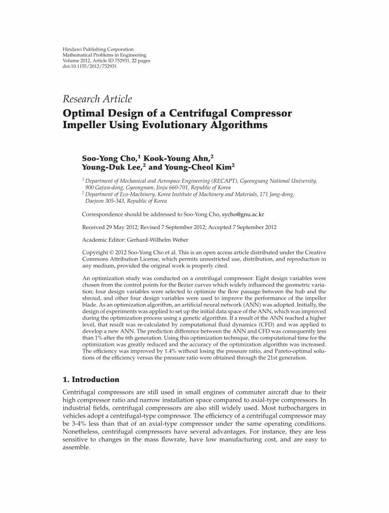
Flow passage of a centrifugal compressor is expressed on the meridian plane. The shape ofa three-dimensional impeller is illustrated by the wrap angle (θ) and the radius, as shownin Figure 1. Profiles of the hub and shroud on the meridian plane can determine the flowpassage, and the infinitesimal length (dm) of the meridional curve with the radius of rref canbe expressed as (2.1). At that location, the blade angle (β) of the impeller can be obtainedusing the wrap angle:

dm =√(dz)2 + (dr)2, (2.1)

β = arctan(rrefdθ

dm

). (2.2)

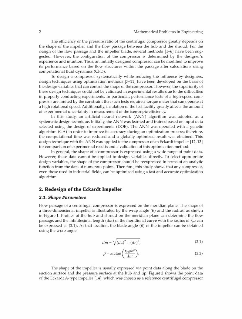
The shape of the impeller is usually expressed via point data along the blade on thesuction surface and the pressure surface at the hub and tip. Figure 2 shows the point dataof the Eckardt A-type impeller [14], which was chosen as a reference centrifugal compressor

Mathematical Problems in Engineering 3

Shroud

m = mmax

Hub

rref

m

z

r

Flow

dmm = 0

(a)

θh(−)

θS(−)

θ(+)

Shroud

Hub

x

y

(b)

Figure 1: Definition of the geometry to illustrate a centrifugal compressor impeller: (a) meridian plane,and (b)wrap angle and Cartesian coordinates.

y (m)−0.16 −0.12 −0.04 0 0.04

x (m

)

0.04

0.06

0.08

0.1

0.12

0.14

0.16

HubTip

−0.08

(a)

z (m)

−0.04 0 0.04 0.08 0.12 0.16

y (m

)

−0.16

−0.12

−0.08

−0.04

0

0.04

HubTip

(b)

Figure 2: Impeller shape as expressed in Cartesian coordinates: (a) on the x-y plane and (b) on the y-zplane.

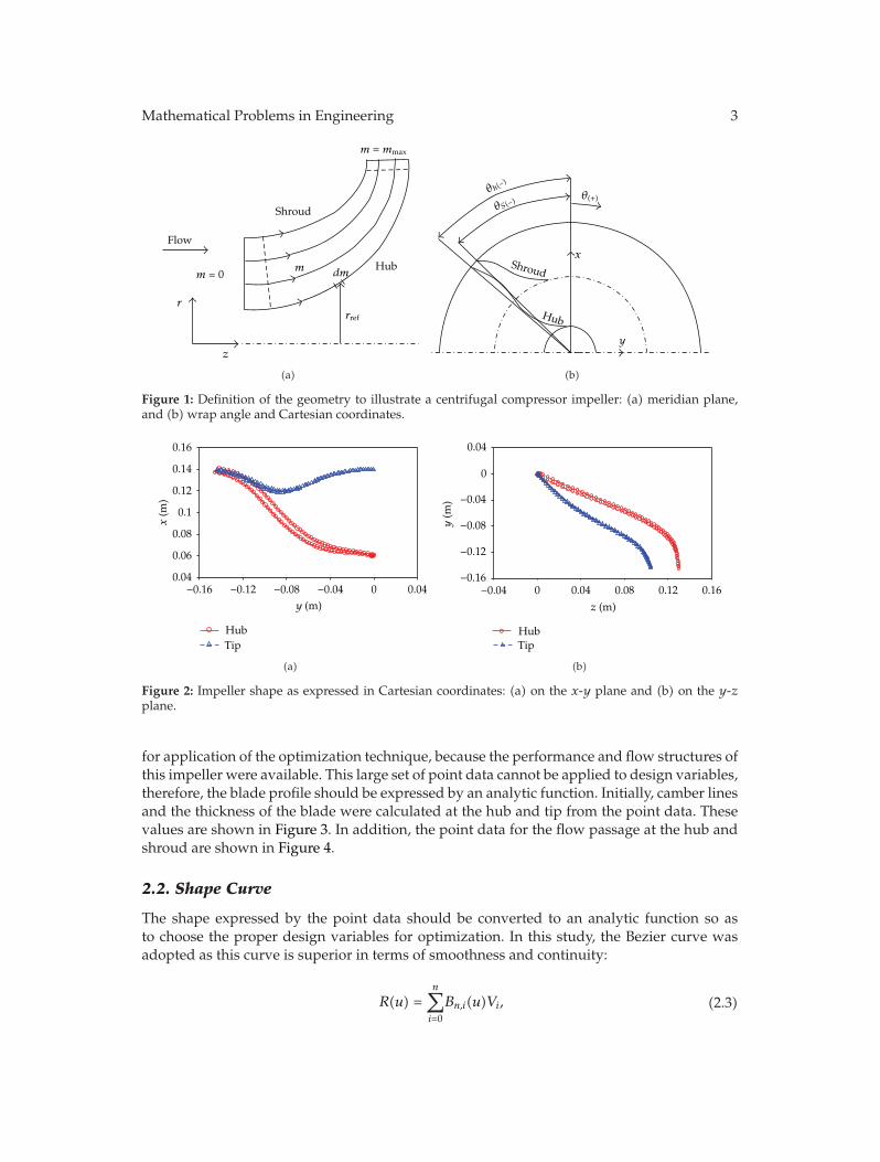
for application of the optimization technique, because the performance and flow structures ofthis impeller were available. This large set of point data cannot be applied to design variables,therefore, the blade profile should be expressed by an analytic function. Initially, camber linesand the thickness of the blade were calculated at the hub and tip from the point data. Thesevalues are shown in Figure 3. In addition, the point data for the flow passage at the hub andshroud are shown in Figure 4.

2.2. Shape Curve

The shape expressed by the point data should be converted to an analytic function so asto choose the proper design variables for optimization. In this study, the Bezier curve wasadopted as this curve is superior in terms of smoothness and continuity:

R(u) =n∑i=0

Bn,i(u)Vi, (2.3)


0

0

0.2 0.4 0.6 0.8 1 1.2

Wra

p an

gle,

θ(r

adia

n)

−1

−0.8

−0.6

−0.4

−0.2

HubTip

Normalized meridional length, λ (m/mmax)

(a)

0 0.2 0.4 0.6 0.8 1 1.2

Th

ick

nes

s (m

m)

0

2

4

6

8

0.2 0.6 1

Th

ick

nes

s (m

m)

0

0.2

0.4

0.6

0.8

1

Hub

Tip

Normalized meridional length, λ(m/mmax)

m (mm)

(b)

Figure 3: Profile of (a) wrap angle and (b) thickness along the camber line of the blade.

where Bn,i(u) is the Bezier coefficient, u is the independent variable, and Vi is the controlpoint. From the given point data, the control points of the Bezier curve can be calculated usingthe matrix of [R] = [B][V ] from (2.3). In this case, additional point data beyond the controlpoints can be applied, and the control points can be obtained by [V ] = {[B]t[B]−1}[B]t[R].However, the slope can change at the ends of the curve depending on the applied point data.Therefore, a boundary condition of the slope was added at the inlet and the exit to connect itsmoothly to the other parts.

⎡⎢⎢⎢⎢⎢⎢⎣

Rk=1

Rk=2...

R′u=0

R′u=1

⎤⎥⎥⎥⎥⎥⎥⎦

=

⎡⎢⎢⎢⎢⎢⎢⎣

Bn,i(uk=1)Bn,i(uk=2)

...n(Bn−1, i−1(0) − Bn,1(0))n(Bn−1, i−1(1) − Bn,1(1))

⎤⎥⎥⎥⎥⎥⎥⎦

⎡⎢⎣Vi=0...

Vi=n

⎤⎥⎦, (2.4)


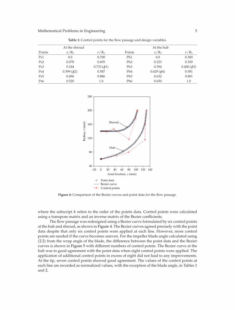
Table 1: Control points for the flow passage and design variables.

At the shroud At the hubPoints z/R2 r/R2 Points z/R2 r/R2

Ps1 0.0 0.700 Ph1 0.0 0.300Ps2 0.078 0.695 Ph2 0.223 0.350Ps3 0.184 0.733 (φ1) Ph3 0.394 0.400 (φ3)Ps4 0.399 (φ2) 0.587 Ph4 0.629 (φ4) 0.581Ps5 0.496 0.886 Ph5 0.632 0.801Ps6 0.520 1.0 Ph6 0.650 1.0

Axial location, z (mm)

−20 0 20 40 60 80 100 120 140

Rad

ius,

r (m

m)

40

80

120

160

200

240

Point dataBezier curveControl points

Shroud

Hub

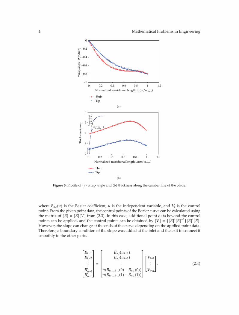
Figure 4: Comparison of the Bezier curves and point data for the flow passage.

where the subscript k refers to the order of the points data. Control points were calculatedusing a transpose matrix and an inverse matrix of the Bezier coefficients.

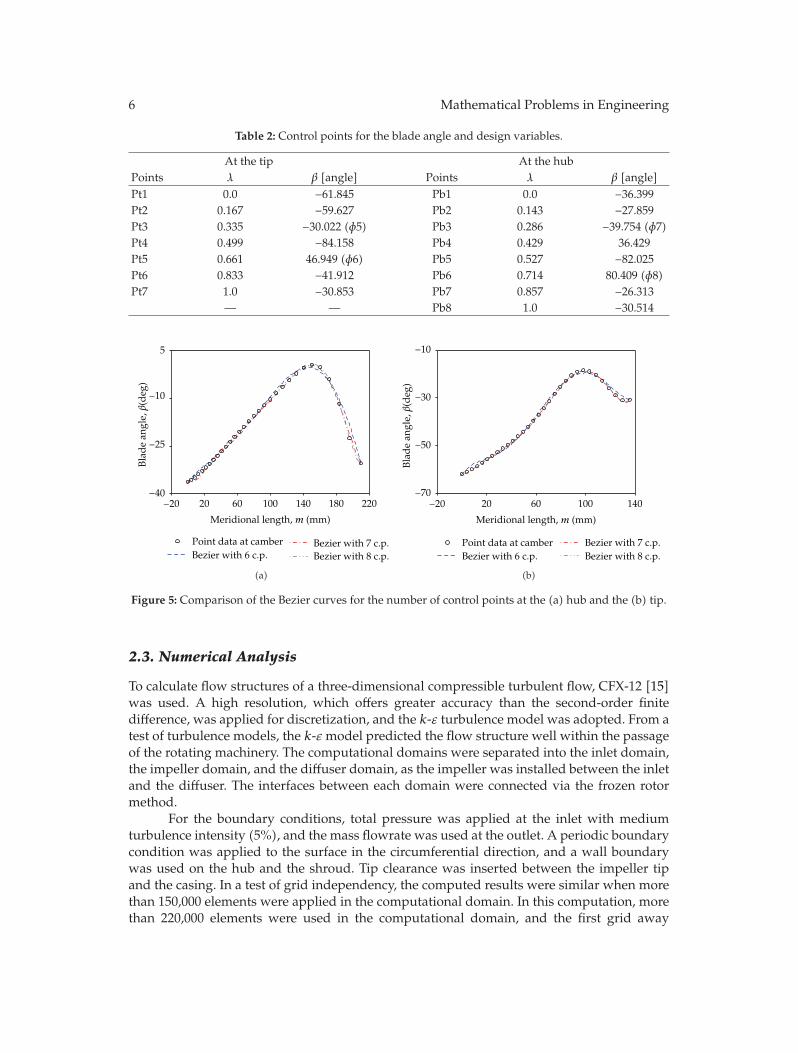
The flow passage was redesigned using a Bezier curve formulated by six control pointsat the hub and shroud, as shown in Figure 4. The Bezier curves agreed precisely with the pointdata despite that only six control points were applied at each line. However, more controlpoints are needed if the curve becomes uneven. For the impeller blade angle calculated using(2.2) from the wrap angle of the blade, the difference between the point data and the Beziercurves is shown in Figure 5 with different numbers of control points. The Bezier curve at thehub was in good agreement with the point data when eight control points were applied. Theapplication of additional control points in excess of eight did not lead to any improvements.At the tip, seven control points showed good agreement. The values of the control points ateach line are recorded as normalized values, with the exception of the blade angle, in Tables 1and 2.


Table 2: Control points for the blade angle and design variables.

At the tip At the hubPoints λ β [angle] Points λ β [angle]Pt1 0.0 −61.845 Pb1 0.0 −36.399Pt2 0.167 −59.627 Pb2 0.143 −27.859Pt3 0.335 −30.022 (φ5) Pb3 0.286 −39.754 (φ7)Pt4 0.499 −84.158 Pb4 0.429 36.429Pt5 0.661 46.949 (φ6) Pb5 0.527 −82.025Pt6 0.833 −41.912 Pb6 0.714 80.409 (φ8)Pt7 1.0 −30.853 Pb7 0.857 −26.313

— — Pb8 1.0 −30.514

−20 20 60 100 140 180 220−40

−25

−10

5

Point data at camberBezier with 6 c.p.

Bezier with 7 c.p.Bezier with 8 c.p.

Meridional length, m (mm)

Bla

de

angl

e, β

(deg

)

(a)

Meridional length, m (mm)

−20 20 60 100 140

Bla

de

angl

e, β

(deg

)

−70

−50

−30

−10

Point data at camberBezier with 6 c.p. Bezier with 8 c.p.

Bezier with 7 c.p.

(b)

Figure 5: Comparison of the Bezier curves for the number of control points at the (a) hub and the (b) tip.

2.3. Numerical Analysis

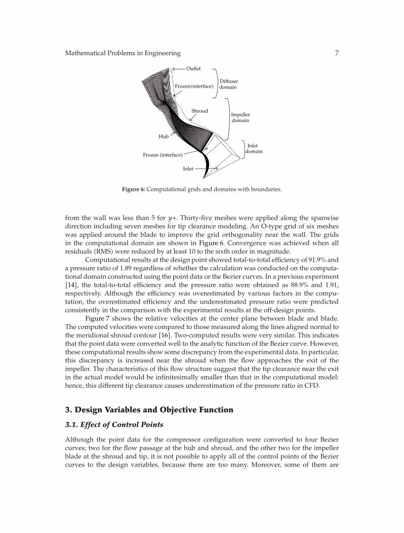
To calculate flow structures of a three-dimensional compressible turbulent flow, CFX-12 [15]was used. A high resolution, which offers greater accuracy than the second-order finitedifference, was applied for discretization, and the k-ε turbulence model was adopted. From atest of turbulence models, the k-ε model predicted the flow structure well within the passageof the rotating machinery. The computational domains were separated into the inlet domain,the impeller domain, and the diffuser domain, as the impeller was installed between the inletand the diffuser. The interfaces between each domain were connected via the frozen rotormethod.

For the boundary conditions, total pressure was applied at the inlet with mediumturbulence intensity (5%), and the mass flowrate was used at the outlet. A periodic boundarycondition was applied to the surface in the circumferential direction, and a wall boundarywas used on the hub and the shroud. Tip clearance was inserted between the impeller tipand the casing. In a test of grid independency, the computed results were similar when morethan 150,000 elements were applied in the computational domain. In this computation, morethan 220,000 elements were used in the computational domain, and the first grid away


Outlet

Diffuserdomain

Impellerdomain

Inletdomain

Inlet

Frozen (interface)

Hub

Shroud

Frozen(interface)

Figure 6: Computational grids and domains with boundaries.

from the wall was less than 5 for y+. Thirty-five meshes were applied along the spanwisedirection including seven meshes for tip clearance modeling. An O-type grid of six mesheswas applied around the blade to improve the grid orthogonality near the wall. The gridsin the computational domain are shown in Figure 6. Convergence was achieved when allresiduals (RMS) were reduced by at least 10 to the sixth order in magnitude.

Computational results at the design point showed total-to-total efficiency of 91.9% anda pressure ratio of 1.89 regardless of whether the calculation was conducted on the computa-tional domain constructed using the point data or the Bezier curves. In a previous experiment[14], the total-to-total efficiency and the pressure ratio were obtained as 88.9% and 1.91,respectively. Although the efficiency was overestimated by various factors in the compu-tation, the overestimated efficiency and the underestimated pressure ratio were predictedconsistently in the comparison with the experimental results at the off-design points.

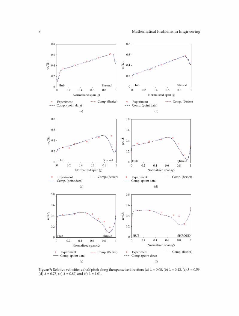
Figure 7 shows the relative velocities at the center plane between blade and blade.The computed velocities were compared to those measured along the lines aligned normal tothe meridional shroud contour [16]. Two-computed results were very similar. This indicatesthat the point data were converted well to the analytic function of the Bezier curve. However,these computational results show some discrepancy from the experimental data. In particular,this discrepancy is increased near the shroud when the flow approaches the exit of theimpeller. The characteristics of this flow structure suggest that the tip clearance near the exitin the actual model would be infinitesimally smaller than that in the computational model:hence, this different tip clearance causes underestimation of the pressure ratio in CFD.

3. Design Variables and Objective Function

3.1. Effect of Control Points

Although the point data for the compressor configuration were converted to four Beziercurves; two for the flow passage at the hub and shroud, and the other two for the impellerblade at the shroud and tip, it is not possible to apply all of the control points of the Beziercurves to the design variables, because there are too many. Moreover, some of them are


Normalized span (ζ)

0 0.2 0.4 0.6 0.8 10

0.2

0.4

0.6

0.8

Hub Shroud

w/U

2

ExperimentComp. (point data)

Comp. (Bezier)

(a)

0 0.2 0.4 0.6 0.8 10

0.2

0.4

0.6

0.8

Hub Shroud


w/U

2


Comp. (Bezier)

(b)

0 0.2 0.4 0.6 0.8 10

0.2

0.4

0.6

0.8

Hub Shroud


w/U

2


Comp. (Bezier)

(c)

0 0.2 0.4 0.6 0.8 10

0.2

0.4

0.6

0.8

Hub Shroud


w/U

2


Comp. (Bezier)

(d)

0 0.2 0.4 0.6 0.8 10

0.2

0.4

0.6

0.8

Hub Shroud



Comp. (Bezier)

w/U

2

(e)

0 0.2 0.4 0.6 0.8 10

0.2

0.4

0.6

0.8

HUB SHROUD



Comp. (Bezier)

w/U

2

(f)

Figure 7:Relative velocities at half pitch along the spanwise direction: (a) λ = 0.08, (b) λ = 0.43, (c) λ = 0.59,(d) λ = 0.73, (e) λ = 0.87, and (f) λ = 1.01.


0 0.2 0.4 0.6 0.8 1

Mov

ing

dis

tanc

e, d

( )

0

0.5

1

1.5

2

Ph3 r-dir.Ph4 r-dir.

Ph3 z-dir.Ph4 z-dir.


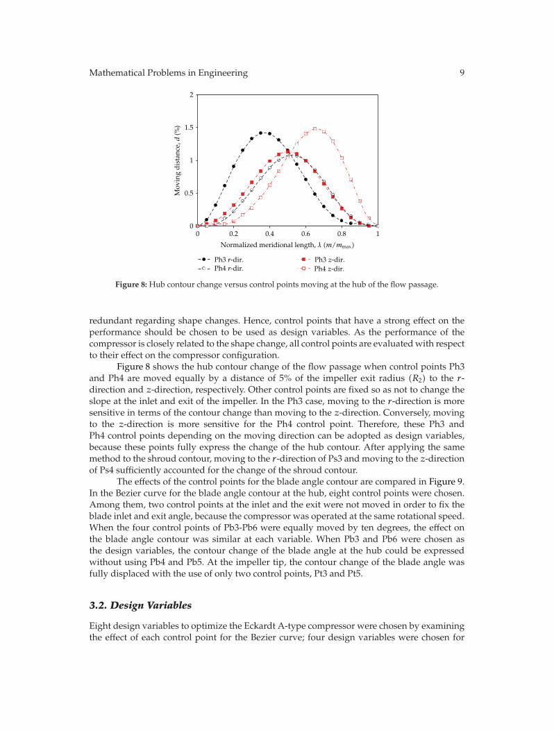
Figure 8: Hub contour change versus control points moving at the hub of the flow passage.

redundant regarding shape changes. Hence, control points that have a strong effect on theperformance should be chosen to be used as design variables. As the performance of thecompressor is closely related to the shape change, all control points are evaluatedwith respectto their effect on the compressor configuration.

Figure 8 shows the hub contour change of the flow passage when control points Ph3and Ph4 are moved equally by a distance of 5% of the impeller exit radius (R2) to the r-direction and z-direction, respectively. Other control points are fixed so as not to change theslope at the inlet and exit of the impeller. In the Ph3 case, moving to the r-direction is moresensitive in terms of the contour change than moving to the z-direction. Conversely, movingto the z-direction is more sensitive for the Ph4 control point. Therefore, these Ph3 andPh4 control points depending on the moving direction can be adopted as design variables,because these points fully express the change of the hub contour. After applying the samemethod to the shroud contour, moving to the r-direction of Ps3 and moving to the z-directionof Ps4 sufficiently accounted for the change of the shroud contour.

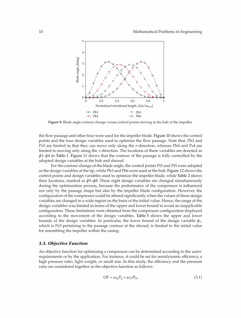
The effects of the control points for the blade angle contour are compared in Figure 9.In the Bezier curve for the blade angle contour at the hub, eight control points were chosen.Among them, two control points at the inlet and the exit were not moved in order to fix theblade inlet and exit angle, because the compressor was operated at the same rotational speed.When the four control points of Pb3-Pb6 were equally moved by ten degrees, the effect onthe blade angle contour was similar at each variable. When Pb3 and Pb6 were chosen asthe design variables, the contour change of the blade angle at the hub could be expressedwithout using Pb4 and Pb5. At the impeller tip, the contour change of the blade angle wasfully displaced with the use of only two control points, Pt3 and Pt5.

3.2. Design Variables

Eight design variables to optimize the Eckardt A-type compressor were chosen by examiningthe effect of each control point for the Bezier curve; four design variables were chosen for


0 0.2 0.4 0.6 0.8 1

Bla

de

angl

e, β

(deg

)

0

1

2

3

4

5

Pb3Pb4

Pb5Pb6

Normalized meridional length, λ[m/mmax]

Figure 9: Blade angle contour change versus control points moving at the hub of the impeller.

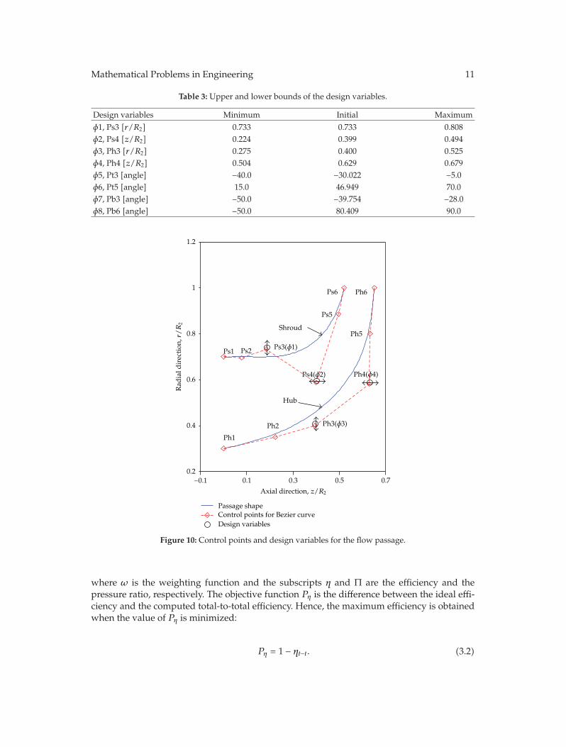
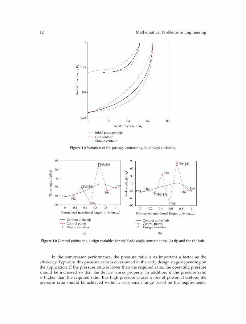
the flow passage and other four were used for the impeller blade. Figure 10 shows the controlpoints and the four design variables used to optimize the flow passage. Note that, Ph3 andPs3 are limited in that they can move only along the r-direction, whereas Ph4 and Ps4 arelimited to moving only along the z-direction. The locations of these variables are denoted asφ1–φ4 in Table 1. Figure 11 shows that the contour of the passage is fully controlled by theadopted design variables at the hub and shroud.

For the contour change of the blade angle, the control points Pt3 and Pt5 were adoptedas the design variables at the tip, while Pb3 and Pb6were used at the hub. Figure 12 shows thecontrol points and design variables used to optimize the impeller blade, while Table 2 showstheir locations, marked as φ5–φ8. These eight design variables are changed simultaneouslyduring the optimization process, because the performance of the compressor is influencednot only by the passage shape but also by the impeller blade configuration. However, theconfiguration of the compressor could be altered significantly when the values of these designvariables are changed in a wide region on the basis of the initial value. Hence, the range of thedesign variables was limited in terms of the upper and lower bound to avoid an inapplicableconfiguration. These limitations were obtained from the compressor configuration displayedaccording to the movement of the design variables. Table 3 shows the upper and lowerbounds of the design variables. In particular, the lower bound of the design variable φ1,which is Ps3 pertaining to the passage contour at the shroud, is limited to the initial valuefor assembling the impeller within the casing.

3.3. Objective Function

An objective function for optimizing a compressor can be determined according to the users’requirements or by the application. For instance, it could be set for aerodynamic efficiency, ahigh pressure ratio, light weight, or small size. In this study, the efficiency and the pressureratio are considered together as the objective function as follows:

OF = ωηPη +ωΠPΠ, (3.1)


Table 3: Upper and lower bounds of the design variables.

Design variables Minimum Initial Maximumφ1, Ps3 [r/R2] 0.733 0.733 0.808φ2, Ps4 [z/R2] 0.224 0.399 0.494φ3, Ph3 [r/R2] 0.275 0.400 0.525φ4, Ph4 [z/R2] 0.504 0.629 0.679φ5, Pt3 [angle] −40.0 −30.022 −5.0φ6, Pt5 [angle] 15.0 46.949 70.0φ7, Pb3 [angle] −50.0 −39.754 −28.0φ8, Pb6 [angle] −50.0 80.409 90.0

−0.1 0.1 0.3 0.5 0.70.2

0.4

0.6

0.8

1

1.2

Passage shapeControl points for Bezier curveDesign variables

Ps1 Ps2

Ps5

Ps6

Ph1

Ph2

Ph5

Ph6

Shroud

Hub

Axial direction, z/R2

Rad

ial d

irec

tion

,r/R

2

Ps3(φ1)

Ps4(φ2) Ph4(φ4)

Ph3(φ3)

Figure 10: Control points and design variables for the flow passage.

where ω is the weighting function and the subscripts η and Π are the efficiency and thepressure ratio, respectively. The objective function Pη is the difference between the ideal effi-ciency and the computed total-to-total efficiency. Hence, the maximum efficiency is obtainedwhen the value of Pη is minimized:

Pη = 1 − ηt−t. (3.2)


0 0.2 0.4 0.6 0.80.25

0.5

0.75

1

Initial passage shapeHub contour Shroud contour

Axial direction, z/R2

Rad

ial d

irec

tion

,r/R

2

Figure 11: Variation of the passage contour by the design variables.

0 0.2 0.4 0.6 0.8 1−90

−60

−30

0

30

60

Contour at the tipControl pointsDesign variables

Pt1Pt2

Pt3(φ5)

Pt5(φ6)

Pt4

Pt6

Pt7


(a)

0 0.2 0.4 0.6 0.8 1−90

−60

−30

0

30

60

90

Contour at the hubControl points Design variables

Pb1Pb2

Pb4

Pb5

Pb7Pb8

Pb6(φ8)

Pb3(φ7)Bla

de

angl

e, β

(deg

)


(b)

Figure 12: Control points and design variables for the blade angle contour at the (a) tip and the (b) hub.

In the compressor performance, the pressure ratio is as important a factor as theefficiency. Typically, this pressure ratio is determined in the early design stage depending onthe application. If the pressure ratio is lower than the required ratio, the operating pressureshould be increased so that the device works properly. In addition, if the pressure ratiois higher than the required ratio, this high pressure causes a loss of power. Therefore, thepressure ratio should be achieved within a very small range based on the requirements.


In this study, this range was set within 1% of the necessary pressure ratio (Πreq). If thecomputed pressure ratio deviates from this range, the objective function of PΠ is increased.Therefore, the efficiency is maximized while the necessary pressure ratio is compromised, asthe objective function (OF) is minimized during the optimization process. In this study, theweighting function was applied equally as one:

PΠ = max

[(∣∣Π −Πreq∣∣

Πreq− 0.01

), 0.0

]. (3.3)

When the impeller shape is changed by various design variables during the optimi-zation process, the impeller may be forced to undergo an unacceptable level of mechanicalstress. In particular, high mechanical stress arises when the impeller is seriously bent. If thismechanical stress is greater than the allowable stress, the impeller will be unfeasible. Thus, aconstraint condition was placed on the mechanical stress as follows:

Pσ =σmax − σallowable

σallowable< 0.0. (3.4)

4. Optimization

4.1. Optimization Method

There are many methods of finding the minimum value of the objective function. As a fastmethod, a gradient-based method can be applied if the objective function rarely reveals non-linear characteristics as a fan. In this case, the gradient-based method would be a good choiceif appropriate initial values are selected so that the optimum does not fall into any localoptimum [17]. However, the objective function on the compressor showed numerous localminimums in the design space. If a gradient-based method is applied to this problem, theresult could be a local minimum. In order to avoid this undesirable result, a response surfacemethod (RSM) [18, 19] or a genetic algorithm (GA) [20, 21] has been applied, but thesemethods often require a considerable amount of computational time depending on the num-ber of design variables. To reduce the computational time, a method that combines the RSMand the GA was introduced [10]. In other methods, the ANN has been applied [22, 23] andthe ANN has been used together with the GA [8, 11, 24]. In addition, the DOE was appliedwith the RSM and the GA [9].

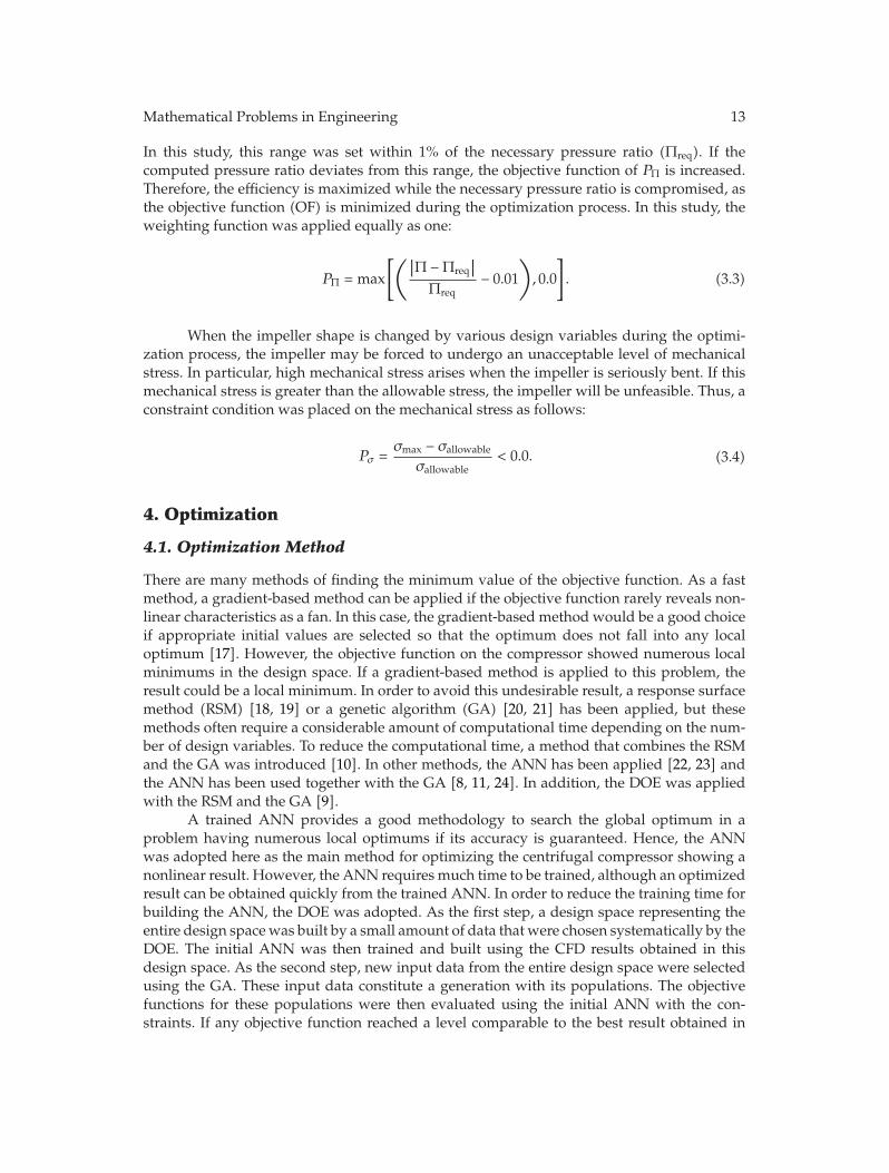
A trained ANN provides a good methodology to search the global optimum in aproblem having numerous local optimums if its accuracy is guaranteed. Hence, the ANNwas adopted here as the main method for optimizing the centrifugal compressor showing anonlinear result. However, the ANN requires much time to be trained, although an optimizedresult can be obtained quickly from the trained ANN. In order to reduce the training time forbuilding the ANN, the DOE was adopted. As the first step, a design space representing theentire design spacewas built by a small amount of data that were chosen systematically by theDOE. The initial ANN was then trained and built using the CFD results obtained in thisdesign space. As the second step, new input data from the entire design space were selectedusing the GA. These input data constitute a generation with its populations. The objectivefunctions for these populations were then evaluated using the initial ANN with the con-straints. If any objective function reached a level comparable to the best result obtained in


Start

Objective functionconstraints

design variables

DOE(design of experiment)

CFDnumerical analysis

TrainingUpdating

GA(genetic algorithm)

Performance

ANN(Artificial neural network)

Stop

Figure 13: Flow chart of optimization.

the previous step, these results were recalculated using the CFD and were then applied toupdate the ANN to increase its accuracy. Therefore, the accuracy of the ANN was con-tinuously improved upon each generation of the GA during the optimization process. Theworking flow for this process is shown in Figure 13.

4.2. Application

The fractional factorial design of 28−2V was applied in the DOE for the data set to train theANN at the beginning. Consequently, the ANN initially required the computed results forsixty-five design cases including a center point. To construct a more accurate ANN, the rangeof the design variables in the DOEwas limited to 75% of the width from the initial value to themaximum or minimum shown in Table 3, because the objective function near the minimumand themaximumwas worse compared to its initial value. However, during the optimizationprocess, the design variables for new design cases were determined over the entire designspace by the GA. For a subsequent generation, the cross-over probability and mutation werechosen as 95% and 10%, respectively.

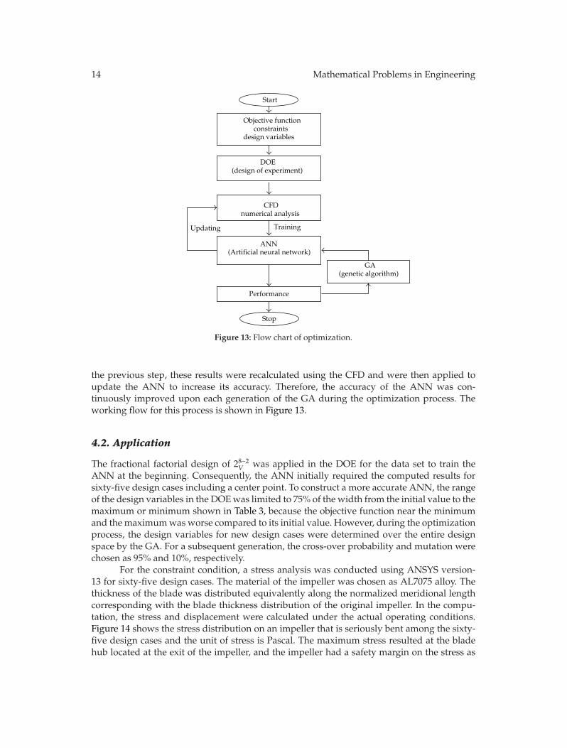
For the constraint condition, a stress analysis was conducted using ANSYS version-13 for sixty-five design cases. The material of the impeller was chosen as AL7075 alloy. Thethickness of the blade was distributed equivalently along the normalized meridional lengthcorresponding with the blade thickness distribution of the original impeller. In the compu-tation, the stress and displacement were calculated under the actual operating conditions.Figure 14 shows the stress distribution on an impeller that is seriously bent among the sixty-five design cases and the unit of stress is Pascal. The maximum stress resulted at the bladehub located at the exit of the impeller, and the impeller had a safety margin on the stress as


1.0941e89.5735e78.2062e76.8389e75.4716e74.1043e72.737e71.3698e7

Max

Min

1.2308e8 Max

24726 Min

Figure 14: Von Mises stresses due to the centrifugal loading.

well as on the displacement for the sixty-five cases. Therefore, the initial ANN was trainedusing the results of the sixty-five cases.

A feedforward backpropagation algorithm with two layers was applied to the ANN.A hyperbolic tangent function and a linear function were applied as a transfer function inthe hidden layer neuron and a transfer function in the output layer neuron, respectively.Ten neurons were used in the hidden layer. The weights and bias vectors of the networkswere searched along the negative gradient of the performance function calculated using theLevernberg-Marquardt algorithm [25, 26]with an initial μ parameter of 0.001. However, theywere updated at a learning rate of 0.1 and a momentum constant of 0.9 so as not to fall ina local minimum while the error, which is the difference between the output predicted bythe neural network and the actual output, was decreasing. The training and learning of thenetwork were conducted using the nntool function in MATLAB [27].

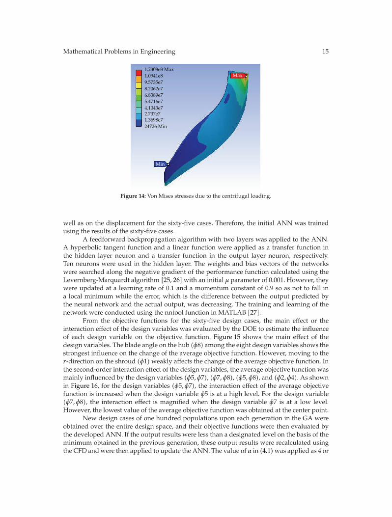
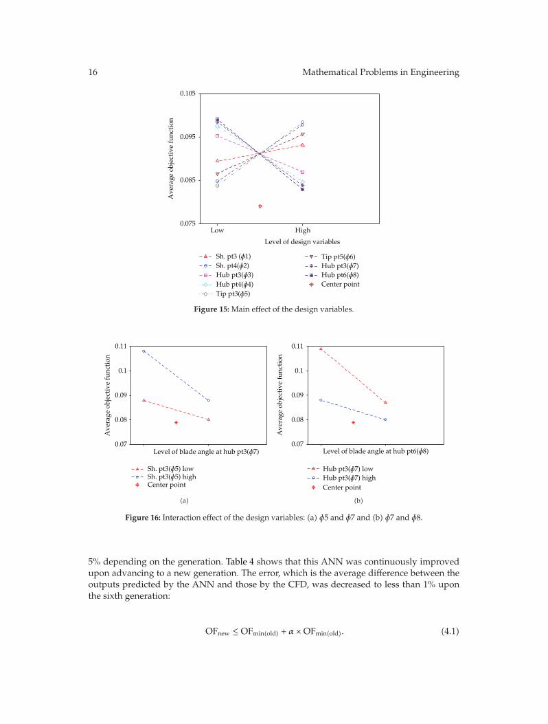
From the objective functions for the sixty-five design cases, the main effect or theinteraction effect of the design variables was evaluated by the DOE to estimate the influenceof each design variable on the objective function. Figure 15 shows the main effect of thedesign variables. The blade angle on the hub (φ8) among the eight design variables shows thestrongest influence on the change of the average objective function. However, moving to ther-direction on the shroud (φ1)weakly affects the change of the average objective function. Inthe second-order interaction effect of the design variables, the average objective function wasmainly influenced by the design variables (φ5, φ7), (φ7, φ8), (φ5, φ8), and (φ2, φ4). As shownin Figure 16, for the design variables (φ5, φ7), the interaction effect of the average objectivefunction is increased when the design variable φ5 is at a high level. For the design variable(φ7, φ8), the interaction effect is magnified when the design variable φ7 is at a low level.However, the lowest value of the average objective function was obtained at the center point.

New design cases of one hundred populations upon each generation in the GA wereobtained over the entire design space, and their objective functions were then evaluated bythe developed ANN. If the output results were less than a designated level on the basis of theminimum obtained in the previous generation, these output results were recalculated usingthe CFD andwere then applied to update the ANN. The value of α in (4.1)was applied as 4 or


Level of design variables

Ave

rage

obj

ecti

ve fu

ncti

on

0.075

0.085

0.095

0.105

Sh. pt3 (φ1)Sh. pt4(φ2) Hub pt3(φ3) Hub pt4(φ4) Tip pt3(φ5)

Tip pt5(φ6) Hub pt3(φ7) Hub pt6(φ8) Center point

Low High

Figure 15: Main effect of the design variables.

Level of blade angle at hub pt3(φ7)

Ave

rage

obj

ecti

ve fu

ncti

on

0.07

0.08

0.09

0.1

0.11

Sh. pt3(φ5) lowSh. pt3(φ5) highCenter point

(a)

Level of blade angle at hub pt6(φ8)

Ave

rage

obj

ecti

ve fu

ncti

on

0.07

0.08

0.09

0.1

0.11

Hub pt3(φ7) lowHub pt3(φ7) highCenter point

(b)

Figure 16: Interaction effect of the design variables: (a) φ5 and φ7 and (b) φ7 and φ8.

5% depending on the generation. Table 4 shows that this ANN was continuously improvedupon advancing to a new generation. The error, which is the average difference between theoutputs predicted by the ANN and those by the CFD, was decreased to less than 1% uponthe sixth generation:

OFnew ≤ OFmin(old) + α ×OFmin(old). (4.1)


Table 4: Number of updated design variables and errors.

Generations Updated design variables Error [%] Level (α) [%]1st 12 8.23 5.02nd 9 3.50 5.03rd 14 3.67 5.04th 8 1.57 5.05th 11 1.60 4.06th 11 0.92 4.0

1.78 1.82 1.86 1.9 1.940.89

0.9

0.91

0.92

0.93

0.94

1.86 1.88 1.9 1.920.926

0.93

0.934

A BC

AB

C

Initial impeller

Pressure ratio, Π

Effi

cien

cy,η

t−t

Figure 17: Paretooptimal solutions of the objective function.

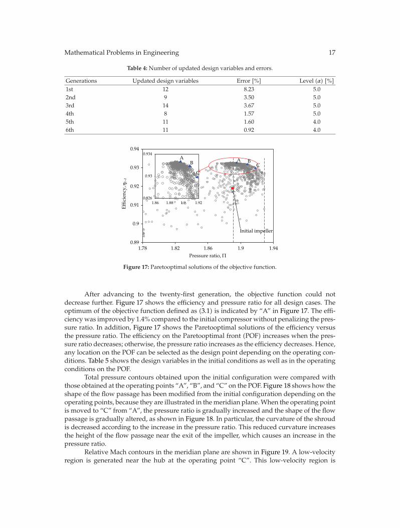
After advancing to the twenty-first generation, the objective function could notdecrease further. Figure 17 shows the efficiency and pressure ratio for all design cases. Theoptimum of the objective function defined as (3.1) is indicated by “A” in Figure 17. The effi-ciencywas improved by 1.4% compared to the initial compressor without penalizing the pres-sure ratio. In addition, Figure 17 shows the Paretooptimal solutions of the efficiency versusthe pressure ratio. The efficiency on the Paretooptimal front (POF) increases when the pres-sure ratio decreases; otherwise, the pressure ratio increases as the efficiency decreases. Hence,any location on the POF can be selected as the design point depending on the operating con-ditions. Table 5 shows the design variables in the initial conditions as well as in the operatingconditions on the POF.

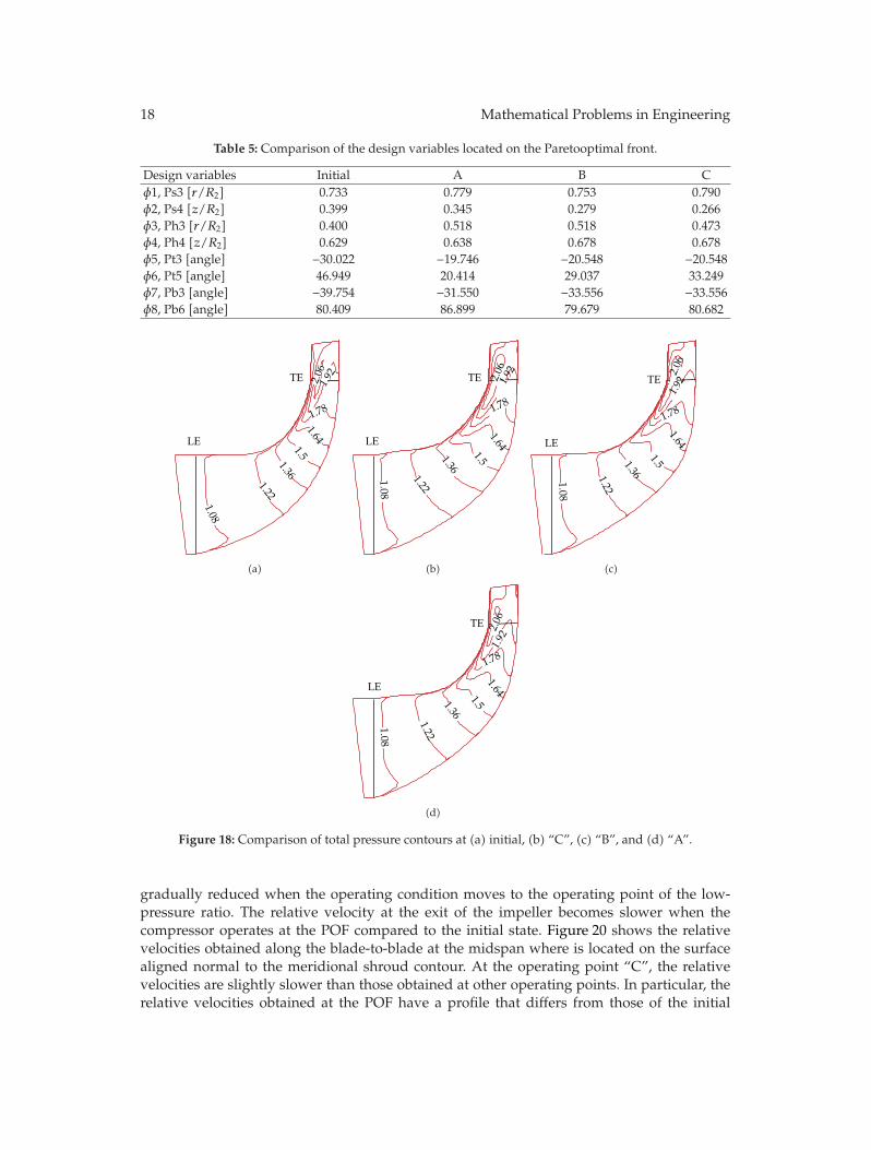
Total pressure contours obtained upon the initial configuration were compared withthose obtained at the operating points “A”, “B”, and “C” on the POF. Figure 18 shows how theshape of the flow passage has been modified from the initial configuration depending on theoperating points, because they are illustrated in themeridian plane.When the operating pointis moved to “C” from “A”, the pressure ratio is gradually increased and the shape of the flowpassage is gradually altered, as shown in Figure 18. In particular, the curvature of the shroudis decreased according to the increase in the pressure ratio. This reduced curvature increasesthe height of the flow passage near the exit of the impeller, which causes an increase in thepressure ratio.

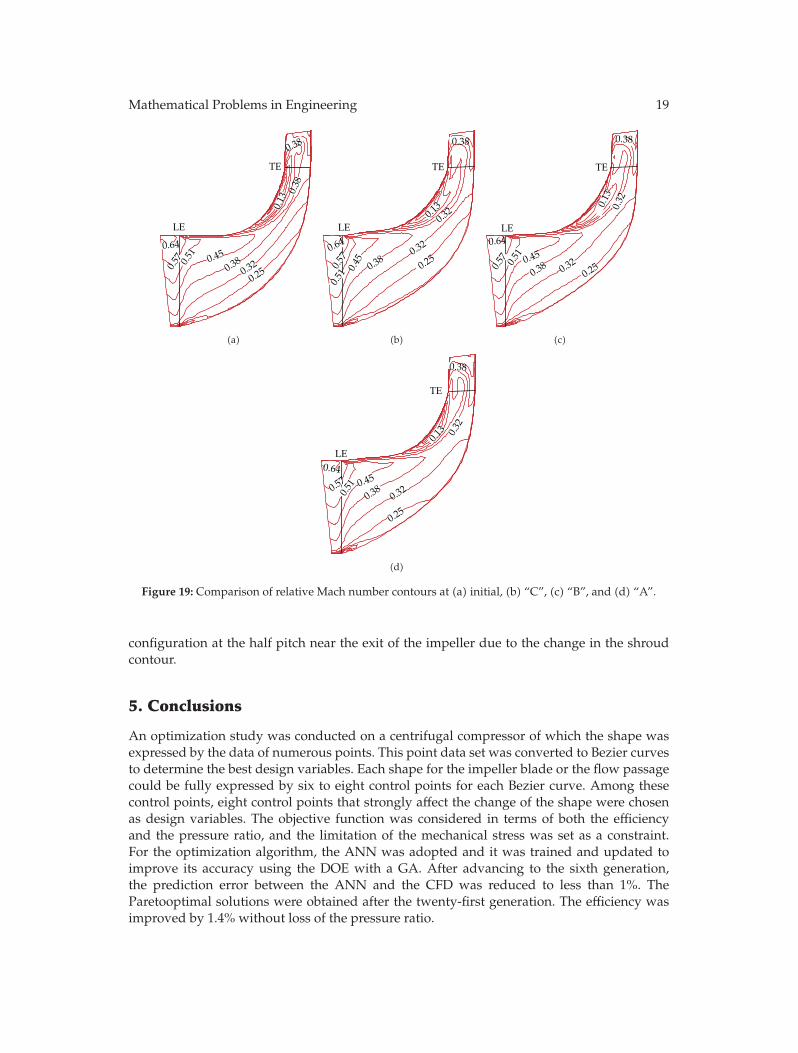
Relative Mach contours in the meridian plane are shown in Figure 19. A low-velocityregion is generated near the hub at the operating point “C”. This low-velocity region is


Table 5: Comparison of the design variables located on the Paretooptimal front.

Design variables Initial A B Cφ1, Ps3 [r/R2] 0.733 0.779 0.753 0.790φ2, Ps4 [z/R2] 0.399 0.345 0.279 0.266φ3, Ph3 [r/R2] 0.400 0.518 0.518 0.473φ4, Ph4 [z/R2] 0.629 0.638 0.678 0.678φ5, Pt3 [angle] −30.022 −19.746 −20.548 −20.548φ6, Pt5 [angle] 46.949 20.414 29.037 33.249φ7, Pb3 [angle] −39.754 −31.550 −33.556 −33.556φ8, Pb6 [angle] 80.409 86.899 79.679 80.682

2.06

1.92

1.78

1.64

1.5

1.36

1.22

1.08

TE

LE

(a)

2.06

1.92

1.78

1.64

1.51.36

1.22

1.08

TE

LE

(b)

2.06

1.92

1.78

1.64

1.51.361.22

1.08

TE

LE

(c)

2.06

1.92

1.78

1.641.51.36

1.22

1.08

TE

LE

(d)

Figure 18: Comparison of total pressure contours at (a) initial, (b) “C”, (c) “B”, and (d) “A”.

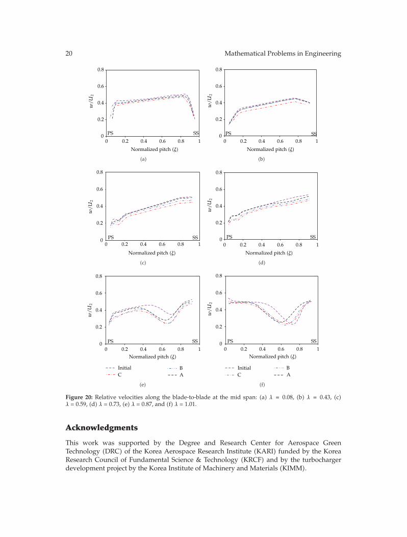
gradually reduced when the operating condition moves to the operating point of the low-pressure ratio. The relative velocity at the exit of the impeller becomes slower when thecompressor operates at the POF compared to the initial state. Figure 20 shows the relativevelocities obtained along the blade-to-blade at the midspan where is located on the surfacealigned normal to the meridional shroud contour. At the operating point “C”, the relativevelocities are slightly slower than those obtained at other operating points. In particular, therelative velocities obtained at the POF have a profile that differs from those of the initial


0.38

0.38

0.380.32

0.250.45

0.64

0.57 0.51

0.13

TE

LE

(a)

0.38

0.32

0.380.32

0.25

0.45

0.64

0.57

0.51

0.13

TE

LE

(b)

0.38

0.32

0.38 0.320.25

0.450.64

0.57 0.51

0.13

TE

LE

(c)

0.38

0.32

0.380.32

0.25

0.450.64

0.57

0.51

0.13

TE

LE

(d)

Figure 19: Comparison of relative Mach number contours at (a) initial, (b) “C”, (c) “B”, and (d) “A”.

configuration at the half pitch near the exit of the impeller due to the change in the shroudcontour.

5. Conclusions

An optimization study was conducted on a centrifugal compressor of which the shape wasexpressed by the data of numerous points. This point data set was converted to Bezier curvesto determine the best design variables. Each shape for the impeller blade or the flow passagecould be fully expressed by six to eight control points for each Bezier curve. Among thesecontrol points, eight control points that strongly affect the change of the shape were chosenas design variables. The objective function was considered in terms of both the efficiencyand the pressure ratio, and the limitation of the mechanical stress was set as a constraint.For the optimization algorithm, the ANN was adopted and it was trained and updated toimprove its accuracy using the DOE with a GA. After advancing to the sixth generation,the prediction error between the ANN and the CFD was reduced to less than 1%. TheParetooptimal solutions were obtained after the twenty-first generation. The efficiency wasimproved by 1.4% without loss of the pressure ratio.


0 0.2 0.4 0.6 0.8 10

0.2

0.4

0.6

0.8

PS SS

w/U

2

Normalized pitch (ξ)

(a)

0 0.2 0.4 0.6 0.8 10

0.2

0.4

0.6

0.8

PS SS

w/U

2


(b)

0 0.2 0.4 0.6 0.8 10

0.2

0.4

0.6

0.8

PS SS

w/U

2


(c)

0 0.2 0.4 0.6 0.8 10

0.2

0.4

0.6

0.8

PS SS

w/U

2


(d)

0 0.2 0.4 0.6 0.8 10

0.2

0.4

0.6

0.8

InitialC

BA

PS SS

w/U

2


(e)

Initial

0 0.2 0.4 0.6 0.8 10

0.2

0.4

0.6

0.8

CBA

PS SS

w/U

2


(f)

Figure 20: Relative velocities along the blade-to-blade at the mid span: (a) λ = 0.08, (b) λ = 0.43, (c)λ = 0.59, (d) λ = 0.73, (e) λ = 0.87, and (f) λ = 1.01.

Acknowledgments

This work was supported by the Degree and Research Center for Aerospace GreenTechnology (DRC) of the Korea Aerospace Research Institute (KARI) funded by the KoreaResearch Council of Fundamental Science & Technology (KRCF) and by the turbochargerdevelopment project by the Korea Institute of Machinery and Materials (KIMM).


References

[1] A. R. Forrest, “Interactive interpolation and approximation by bezier polynomials,” Computer Journal,vol. 15, no. 1, pp. 71–79, 1972.

[2] F. J. Wallace, A. Whitfield, and R. Atkey, “A computer-aided design procedure for radial and mixedflow compressors,” Computer-Aided Design, vol. 7, no. 3, pp. 163–170, 1975.

[3] M. V. Casey, “A computational geometry for the blades and internal flow channels of centrifugal com-pressors,” Journal of Engineering for Power, vol. 105, no. 2, pp. 288–295, 1983.

[4] N. A. Cumpsty, Compressor Aerodynamics, Longman Group UK, 1989.[5] A. Whitfield and N. C. Baines, Design of Radial Turbomachines, Longman Group UK, 1990.[6] R. H. Aungier, Centrifugal Compressor, ASME Press, 2000.[7] D. Bonaiuti and V. Pediroda, “Aerodynamic optimization of an industrial centrifugal compressor

impeller using genetic algorithms,” in Proceedings of Eurogen, 2001.[8] R. Cosentino, Z. Alsalihi, and V. R. A. Braembussche, “Expert system for radial impeller optimi-

zation,” in Proceedings of Euroturbo, 2001.[9] D. Bonaiuti, A. Arnone, M. Ermini, and L. Baldassarre, “Analysis and optimization of transonic

centrifugal compressor impellers using the design of experimental technique,” GT-2002-30619, 2002.[10] D. Bonaiuti and M. Zangeneh, “On the coupling of inverse design and optimization techniques for

the multiobjective, multipoint design of turbomachinery blades,” Journal of Turbomachinery, vol. 131,no. 2, Article ID 021014, 16 pages, 2009.

[11] T. Verstraete, Z. Alsalihi, and R. A. Van den, “Multidisciplinary optimization of a radial compressorformicrogas turbine applications,” Journal of Turbomachinery, vol. 132, no. 3, Article ID 031004, 7 pages,2010.

[12] D. Eckardt, “Instantaneous measurements in the jet-wake discharge flow of a centrifugal compressorimpeller,” Journal of Engineering and Power, vol. 97, no. 3, pp. 337–346, 1975.

[13] D. Eckardt, “Detailed flow investigations within a high-speed centrifugal compressor impeller,”Journal of Fluid Engineering, vol. 98, no. 3, pp. 390–402, 1976.

[14] D. Eckardt, “Flowfield analysis of radial and backswept centrifugal compressor impellers—part 1:flow measurements using a laser velocimeter,” in Performance Prediction of Centrifugal Pumps andCompressor, S. Gopalskrishnan and P. Cooper, Eds., ASME, 1980.

[15] CFX-12, version 12, Ansys Inc, 2009.[16] P. Schuster and U. Schmidt-Eisenlohr, “Flowfield analysis of radial and backswept centrifugal com-

pressor impellers—part 2: comparison of potential flow calculations and measurements,” in Perfor-mance Prediction of Centrifugal Pumps and Compressor, S. Gopalskrishnan and P. Cooper, Eds., ASME,1980.

[17] C. H. Cho, S. Y. Cho, K. Y. Ahn, and Y. C. Kim, “Study of an axial-type fan design technique usingan optimization method,” Proceedings IMechE Journal of Process Mechanical Engineering, vol. 223, no. 3,pp. 101–111, 2009.

[18] Z. Wang, G. Xi, and X. Wang, “Aerodynamics design optimization of vaned diffuser for centrifugalcompressors using Kriging model,” in Proceeding of Asian Joint Conference on Propulsion and Power(AJCPP ’06), Beijing, China, 2006.

[19] X. Shu, C. Gu, J. Xiao, and C. Gao, “Centrifugal compressor blade optimization based on uniformdesign and genetic algorithms,” Frontiers of Energy and Power Engineering in China, vol. 2, no. 4, pp.453–456, 2008.

[20] H. Y. Fan, “An inverse design method of diffuser blades by genetic algorithms,” Proceedings IMechEJournal of Power and Energy, vol. 212, no. 4, pp. 261–268, 1998.

[21] E. Benini, “Optimal Navier-Stokes design of Ccompressor impellers using evolutionary computa-tion,” International Journal of Computational Fluid Dynamics, vol. 17, no. 5, pp. 357–369, 2003.

[22] S. Pierret and R. A. Van Den Braembussche, “Turbomachinery blade design using a Navier-Stokessolver and Artificial Neural Network,” Journal of Turbomachinery, vol. 121, no. 2, pp. 326–332, 1999.

[23] H. Y. Fan, “A neural network approach for centrifugal impeller inverse design,” Proceedings IMechEJournal of Power and Energy, vol. 214, no. 2, pp. 183–186, 2000.

[24] J. H. Kim, J. H. Choi, A. Husain, and K. Y. Kim, “Multi-objective optimization of a centrifugal com-pressor impeller through evolutionary algorithms,” Proceedings IMechE Journal of Power and Energy,vol. 224, no. 5, pp. 711–721, 2010.


[25] M. T. Hagan and M. B. Menhaj, “Training feedforward networks with the Marquardt algorithm,”IEEE Transactions on Neural Networks, vol. 5, no. 6, pp. 989–993, 1994.

[26] M. T. Hagan, H. B. Demuth, and M. H. Beale, Neural Network Design, PWS Publishing, Boston, Mass,USA, 1996.

[27] H. Demuth, M. Beale, andM. Haga, “Neural Network Toolbox 6, User’s Guide,”Matlab R2007b, 2007.

Submit your manuscripts athttp://www.hindawi.com

Hindawi Publishing Corporationhttp://www.hindawi.com Volume 2014

MathematicsJournal of


Mathematical Problems in Engineering

Hindawi Publishing Corporationhttp://www.hindawi.com

Differential EquationsInternational Journal of

Volume 2014

Applied MathematicsJournal of


Probability and StatisticsHindawi Publishing Corporationhttp://www.hindawi.com Volume 2014

Journal of


Mathematical PhysicsAdvances in

Complex AnalysisJournal of


OptimizationJournal of


CombinatoricsHindawi Publishing Corporationhttp://www.hindawi.com Volume 2014

International Journal of


Operations ResearchAdvances in

Journal of


Function Spaces

Abstract and Applied AnalysisHindawi Publishing Corporationhttp://www.hindawi.com Volume 2014

International Journal of Mathematics and Mathematical Sciences


The Scientific World JournalHindawi Publishing Corporation http://www.hindawi.com Volume 2014


Algebra

Discrete Dynamics in Nature and Society



Decision SciencesAdvances in

Discrete MathematicsJournal of

Hindawi Publishing Corporationhttp://www.hindawi.com

Volume 2014


Stochastic AnalysisInternational Journal of

Optimal Design of a Centrifugal Compressor Impeller Using … · 2014-04-24 · Optimal Design of a...

Documents

Transcript of Optimal Design of a Centrifugal Compressor Impeller Using … · 2014-04-24 · Optimal Design of a...