Optimal Debt Maturity and Firm Investment

ADEMU WORKING PAPER SERIES

Optimal Debt Maturity and Firm Investment*

Joachim Jungherr† Immo SchottŦ

November 2016

WP 2016/051 www.ademu-project.eu/publications/working-papers

Abstract This paper introduces a maturity choice to the standard model of firm financing and investment. Long-term debt renders the optimal firm policy time-inconsistent. Lack of commitment gives rise to debt dilution. This problem becomes more severe during downturns. We show that cyclical debt dilution generates the observed counter-cyclical behavior of default, bond spreads, leverage, and debt maturity. It also generates the pro-cyclical term structure of corporate bond spreads. Debt dilution renders the equilibrium outcome constrained-inefficient: credit spreads are too high and investment is too low. In two policy experiments we find the following: (1) an outright ban of long-term debt improves welfare in our model economy, and (2.) debt dilution accounts for 84% of the credit spread and 25% of the welfare gap with respect to the first best allocation.

Keywords: firm financing, investment, debt maturity, credit spreads, debt dilution

JEL codes: E22, E32, E44, G32

∗ A previous version of this paper circulated under the title “Cyclical Debt Dilution”. _________________________

† Institut d’Analisi Economica (CSIC), MOVE, and Barcelona GSE Email: [email protected] Ŧ Universite de Montreal and CIREQ Email: [email protected]

http://www.ademu-project.eu/publications/working-papers

mailto:[email protected]

mailto:[email protected]

Acknowledgments We appreciate helpful comments by Christian Bayer, Gian Luca Clementi, Simon Gilchrist, Jonathan Heathcote, Andrea Lanteri, Albert Marcet, Claudio Michelacci, Juan Pablo Nicolini, and participants of various seminars and conference presentations. Joachim Jungherr is grateful for financial support from the ADEMU project (A Dynamic Economic and Monetary Union) funded by the European Union (Horizon 2020 Grant 649396), from the Spanish Ministry of Economy and Competitiveness through the Severo Ochoa Programme for Centres of Excellence in R&D (SEV-2015-0563) and through Grant ECO2013-48884-C3-1P, and from the Generalitat de Catalunya (Grant 2014 SGR 1432) _________________________

The ADEMU Working Paper Series is being supported by the European Commission Horizon 2020 European Union funding for Research & Innovation, grant agreement No 649396.

This is an Open Access article distributed under the terms of the Creative Commons Attribution License Creative Commons Attribution 4.0 International, which permits unrestricted use, distribution and reproduction in any medium provided that the original work is properly attributed.

1. Introduction

Borrowing costs for U.S. firms increased dramatically during the Great Recession. Thedefault rate on corporate bonds increased from 0.13% in 2007 to 2.48% in 2009.1 Whatdrives these fluctuations in credit spreads and default rates? The standard approach inthe literature is to address this question using a model of one-period debt. Empirically,firms rely heavily on long-term debt.2 This paper studies the link between credit marketfrictions and economic activity using a model in which firms are allowed to issue bothshort-term and long-term liabilities.

In our model, firms choose leverage by trading off the tax advantage of debt againstthe potential cost of default. Firms also choose the maturity of their debt. Short-termdebt has the disadvantage that its entire amount needs to be rolled-over each period.This is costly because of a transaction cost on the bond market.

Our model replicates the stylized facts of U.S. firm financing.3 Default rates, bondspreads, leverage, and debt maturity all increase during downturns. At the same time,the difference between long-term and short-term bond spreads (the term structure) falls.This paper shows that a single economic mechanism can account for these empirical facts:Cyclical debt dilution.

Debt dilution arises because long-term debt renders the optimal debt issuance policytime-inconsistent.4 The firm disregards part of the total potential costs of default,because it does not internalize the effect of its actions on the value of previously issuedbonds. Through this mechanism, debt dilution induces the firm to lever up. Higherleverage increases the risk of default at any point of the business cycle.

A novel result of our paper is that the intensity of debt dilution varies over the businesscycle. During recessions, investment and the amount of newly issued debt are low, butthe ratio of previously issued debt to newly issued debt is high. Because the firmdisregards a large fraction of the total potential costs of default, it chooses to run aparticularly high risk of default during downturns. As we show below, this renders thedefault rate, credit spreads, leverage, and debt maturity counter-cyclical.

While the equilibrium in a model of one-period debt is constrained-efficient, this isno longer true once we allow firms to issue both short-term and long-term liabilities.

1Gilchrist and Zakrajsek (2012) measure an increase in the average credit spread over U.S. treasuriesfrom less than 1.5 percentage points in 2007 to almost 8 percentage points in 2009 for a sample of 5,982senior unsecured bonds issued by non-financial firms. Adrian, Colla, and Shin (2012) document for adifferent sample that the average cost of newly issued bonds increased from about 1.5 percentage pointsin 2007 to more than 4 percentage points in 2009. Data on default rates is from Giesecke, Longstaff,Schaefer, and Strebulaev (2014).

2For U.S. non-financial corporate firms 1984-2016, the average share of long-term liabilities (withterm to maturity above on year) is 67%. Gilchrist and Zakrajsek (2012) measure for the years 1973-2011an average term to maturity of long-term bonds of 11.3 years. Adrian et al. (2012) find that the averagematurity of all newly issued bonds fluctuates 1998-2011 between roughly 5 and 15 years.

3We present the cyclical patterns of U.S. corporate firm financing in Section 3.4Debt dilution also plays a key role in quantitative models of sovereign debt. See Arellano and

Ramanarayanan (2012), Chatterjee and Eyigungor (2012), or Hatchondo, Martinez, and Sosa-Padilla(2016). Bonds issued by U.S. firms commonly include debt covenants which restrict firm policy. InSection 5.5.4, we provide an overview of empirically observed types of debt covenants.

1

Debt dilution renders the equilibrium outcome constrained-inefficient. Future borrowingexerts an externality on the buyers of newly issued long-term debt. Rational investorspay lower bond prices because firms cannot commit to abstain from debt dilution in thefuture. Since spreads are inefficiently high, investment is inefficiently low.

The contribution of our paper can be broken down into three parts. In the first part ofthe paper, we use a simple two-period model to derive analytical results on the cyclicalrole of debt dilution in driving credit spreads and default rates. We use these analyticalresults to interpret the numerical findings of our fully dynamic model economy. In ourview, these analytical results are also helpful to interpret other numerical findings fromthe emerging literature on long-term debt (e.g. Gomes, Jermann, and Schmid (2016)).

Models of long-term debt often are solved using an ‘inner loop/outer loop’ procedure.This involves computing the complete bond price schedule for all possible states andactions. This price schedule is then used to compute the optimal policy (e.g. Hatchondoand Martinez (2009)). As a second contribution of our paper, we re-formulate the firmproblem in a way which expresses equilibrium bond prices as a function of choice variablesand future firm policy. Equilibrium bond prices and today’s firm policy are computedin a single step. This reduces the number of necessary computations and allows for afaster and more precise solution.

The third contribution of our paper is quantitative. Within a fully dynamic economy,we show that cyclical debt dilution generates the observed counter-cyclical behavior ofdefault, bond spreads, leverage, and debt maturity. It also generates the pro-cyclicalterm structure of corporate bond spreads. We consider two policy experiments whichboth eliminate debt dilution: (1.) a ban of long-term debt, and (2.) a debt covenantwhich helps firms to internalize the cost of debt dilution. Both policies improve welfare byreducing credit spreads and increasing investment. We find that debt dilution accountsfor 84% of the credit spread and 25% of the welfare gap with respect to the first bestallocation. The welfare gain from eliminating debt dilution corresponds to a decrease inthe corporate tax rate of 2.5 percentage points.

In Section 2 we briefly survey some related literature. Section 3 documents the stylizedfacts of cyclical U.S. corporate firm financing. In Section 4 we describe a two-periodeconomy and derive analytical results on the cyclical role of debt dilution. We usethese results to interpret our findings from a fully dynamic model economy presentedin Section 5. We describe an efficient solution method for this model and study itsbehavior. We focus on firms’ response to aggregate shocks and the welfare cost of debtdilution. Concluding remarks follow. Formal proofs are deferred to the appendix.

2. Related Literature

To the best of our knowledge, firms’ optimal maturity choice over the business cycle hasnot been formally studied before. We aim at closing this gap in the literature and findthat debt dilution plays a key role for this trade-off.

While the choice between short-term debt and long-term debt is usually absent frommodels of firm financing and investment, several papers consider an exogenous maturity

2

structure with long-term debt. In Gomes and Schmid (2016), firms are required to buyback previously issued long-term bonds before issuing new debt. Caggese and Perez(2015) assume that debt is fixed over the life-span of the firm. Setups like these rule outdebt dilution by assumption.

Also Miao and Wang (2010) and Gourio and Michaux (2012) study a firm problemwith long-term debt. The authors present numerical results on the counter-cyclicalityof credit spreads and default without an explicit discussion of debt dilution. We con-tribute analytical and numerical results which identify the cyclical role of debt dilution.Identifying this role is important because it allows to assess the potential benefits ofpolicy measures which help firms overcome their time-inconsistency problem. A secondimportant difference to our model is that these papers do not consider short-term debt.This assumption is restrictive since a maturity choice allows firms to respond to andmitigate distortions which arise from long-term debt.

In a model with nominal debt, Gomes et al. (2016) show that shocks to inflationchange the real burden of long-term debt and thereby distort investment decisions. Asin Miao and Wang (2010) and Gourio and Michaux (2012), the role of debt dilution isnot explicitly discussed and there is no maturity choice. At the end of section 4.4.3, webriefly discuss how our analytical results relate to the numerical findings from Gomeset al. (2016).

As an exception with respect to the rest of the literature, Crouzet (2016) studies amodel in which firms have access both to short-term and long-term debt. In contrast toour paper, firms cannot raise funds by selling equity. Furthermore, the author studiesa stationary distribution of firms, whereas we study firms’ maturity choice over thebusiness cycle.

We find that debt dilution generates counter-cyclical credit spreads and default rates.Many models without long-term debt do not share this feature. Gomes, Yaron, andZhang (2003) show that the financial accelerator model without equity issuance (e.g.Carlstrom and Fuerst (1997)) generates a pro-cyclical default rate.5 Covas and Den Haan(2012) find a pro-cyclical default rate in a model with costly equity issuance.

While the role of debt dilution has not been explored by the literature on firm financingand investment, it has enjoyed a lot of attention from the literature on sovereign debt.Sachs and Cohen (1982) illustrate debt dilution in a three-period model. A recent waveof quantitative studies finds that debt dilution is important to explain the magnitudeand the volatility of credit spreads on sovereign debt. Hatchondo and Martinez (2009)numerically show that debt dilution amplifies the cyclicality of spreads. In Chatterjeeand Eyigungor (2012), a sovereign borrower uses long-term debt in spite of debt dilutionto reduce the risk of rollover crises. Using a similar setup, Hatchondo and Martinez(2013) find that the optimal maturity choice itself is time-inconsistent. This is alsotrue in our model. Aguiar, Amador, Hopenhayn, and Werning (2016) study a model ofsovereign debt in which the competitive equilibrium allocation is Pareto-efficient onceone disregards the owners of outstanding long-term debt. Chatterjee and Eyigungor(2015) propose a computationally tractable seniority arrangement. Hatchondo et al.

5See also the discussion of the costly state verification model in Quadrini (2011).

3

(2016) quantify the welfare benefits from different debt covenants.Arellano and Ramanarayanan (2012) report that the maturity of sovereign debt short-

ens if spreads increase. Their model generates this pattern because they assume thatthe exogenous default punishment falls during downturns. This shifts the bond priceschedules and reduces the endogenous debt limit in a way which favors short-term debt.In our model, the maturity of firm debt rises if spreads increase. This is because ourmodel does not feature a default punishment which is exogenously tied to the businesscycle. Spreads and debt maturity only move over the business cycle because of debtdilution. The ratio of old debt to new debt increases during downturns. Debt dilutionbecomes stronger which causes both spreads and debt maturity to increase in our model.

The models on sovereign debt cited above are endowment economies. Debt dilutionaffects credit spreads but these spreads do not affect output. In our model, spreadsaffect firm investment and output. For this reason, the impact of debt dilution onwelfare is very different. Furthermore, models of sovereign debt generate counter-cyclicalspreads through an exogenous pro-cyclical default punishment. In contrast, we study aproduction economy and analytically demonstrate that debt dilution alone can generatecounter-cyclical credit spreads. Endogenous investment is key for this mechanism.

3. Empirical Facts

In this section, we document the business cycle behavior of several financial variablesfor non-financial corporate firms in the US. As recommended by Jermann and Quadrini(2012), we include observations starting in the first quarter of 1984.6

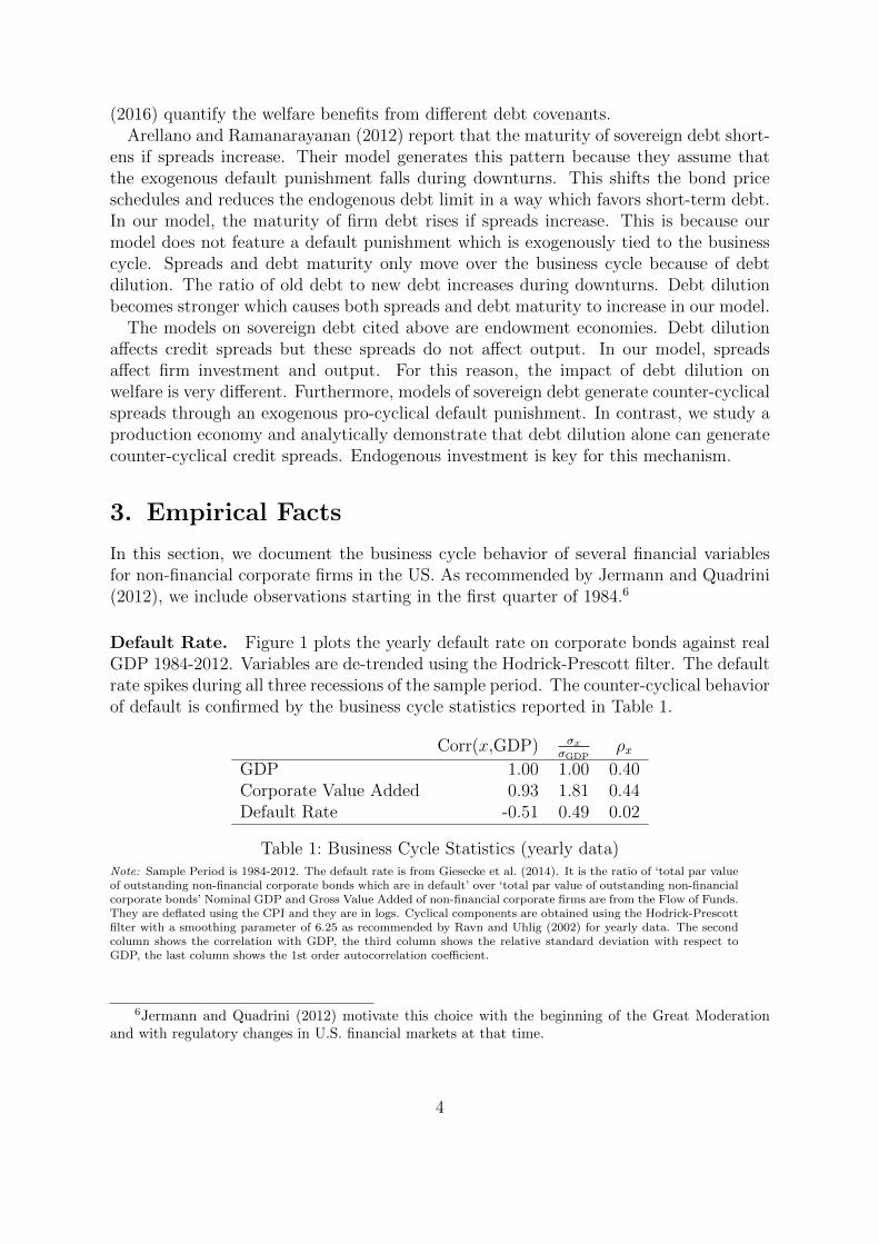
Default Rate. Figure 1 plots the yearly default rate on corporate bonds against realGDP 1984-2012. Variables are de-trended using the Hodrick-Prescott filter. The defaultrate spikes during all three recessions of the sample period. The counter-cyclical behaviorof default is confirmed by the business cycle statistics reported in Table 1.

Corr(x,GDP) σxσGDP

ρxGDP 1.00 1.00 0.40Corporate Value Added 0.93 1.81 0.44Default Rate -0.51 0.49 0.02

Table 1: Business Cycle Statistics (yearly data)Note: Sample Period is 1984-2012. The default rate is from Giesecke et al. (2014). It is the ratio of ‘total par valueof outstanding non-financial corporate bonds which are in default’ over ‘total par value of outstanding non-financialcorporate bonds’ Nominal GDP and Gross Value Added of non-financial corporate firms are from the Flow of Funds.They are deflated using the CPI and they are in logs. Cyclical components are obtained using the Hodrick-Prescottfilter with a smoothing parameter of 6.25 as recommended by Ravn and Uhlig (2002) for yearly data. The secondcolumn shows the correlation with GDP, the third column shows the relative standard deviation with respect toGDP, the last column shows the 1st order autocorrelation coefficient.

6Jermann and Quadrini (2012) motivate this choice with the beginning of the Great Moderationand with regulatory changes in U.S. financial markets at that time.

4

−.0

050

.005

.01

.015

Def

ault

Rat

e (c

yclic

al c

ompo

nent

)

−.0

2−

.01

0.0

1.0

2lo

g R

eal G

DP

(cy

clic

al c

ompo

nent

)

1985 1990 1995 2000 2005 2010Year

GDP Default Rate

Figure 1: Corporate Default Rate over the Business Cycle.Note: The default rate is from Giesecke et al. (2014). It is the ratio of ’total par value of outstanding non-financialcorporate bonds which are in default’ over ’total par value of outstanding non-financial corporate bonds’. NominalGDP is from the Flow of Funds. Real GDP is calculated using the Consumer Price Index from the Bureau ofLabor Statistics. It is in logs. Cyclical components are obtained using the Hodrick-Prescott filter with a smoothingparameter of 6.25 as recommended by Ravn and Uhlig (2002) for yearly data.

Leverage. For all remaining variables data is available on a quarterly frequency. Theupper panel of Figure 2 plots corporate leverage over the business cycle. Leverage isdefined as total liabilities as a fraction of total assets. Especially during the time period2000-2011, a strong negative co-movement between output and leverage is apparent.During recent downturns, corporate firms have reduced their assets faster than theirliabilities. This has caused leverage to rise in recessions. In Table 2 we calculate busi-ness cycle statistics using yearly data 1984-2015.7 The correlation between output andleverage is −0.75.

Long-term Liabilities Share. In the lower panel of Figure 2 the maturity struc-ture of corporate liabilities is plotted against the business cycle. It shows long-termliabilities (with remaining maturity of more than one year) as a fraction of total corpo-rate liabilities. During downturns, the share of long-term liabilities increases sharply asfirms reduce short-term liabilities faster than their long-term liabilities. Table 2 showsa correlation between output and the share of long-term liabilities of −0.69.

Corporate Bond Spreads. Data on corporate bond spreads is only available startingfrom the first quarter of 1997. The upper panel of Figure 3 shows how yields on corporate

7In our numerical exercise in Section 5, the model period is a year. In order to compare ourquantitative findings with the data, we calculate business cycle statistics using yearly data.

5

−.0

50

.05

log

Liab

ilitie

s / A

sset

s (c

yclic

al c

ompo

nent

)

−.0

20

.02

log

Rea

l GD

P (

cycl

ical

com

pone

nt)

1985q1 1990q1 1995q1 2000q1 2005q1 2010q1 2015q1Quarter

NBER Recession GDPLiabilities / Assets

−.0

20

.02

Log

Sha

re o

f Lon

g−te

rm L

iabi

litie

s (c

ycl.

com

p.)

−.0

20

.02

log

Rea

l GD

P (

cycl

ical

com

pone

nt)

1985q1 1990q1 1995q1 2000q1 2005q1 2010q1 2015q1Quarter

NBER Recession GDPShare of Long−term Liabilities

Figure 2: Leverage and the Share of Long-term Liabilities.Note: Total Assets, Short-term Liabilities, and Total Liabilities of non-financial corporate firms are from the Flow ofFunds. Variables are in logs. Cyclical components are obtained using the Hodrick-Prescott filter with a smoothingparameter of 1600. Grey bars indicate NBER recessions.

6


ρxGDP 1.00 1.00 0.42Corporate Value Added 0.95 1.77 0.47Corporate Investment 0.76 4.39 0.44Liabilities / Assets -0.75 1.95 0.30Long-term Liabilities Share -0.69 1.47 0.33

Table 2: Business Cycle Statistics (yearly data)Note: Sample Period is 1984-2015. All variables are from the Flow of Funds. They deflated using the CPI and theyare in logs. Cyclical components are obtained using the Hodrick-Prescott filter with a smoothing parameter of 6.25.The second column shows the correlation with GDP, the third column shows the relative standard deviation withrespect to GDP, the last column shows the 1st order autocorrelation coefficient.

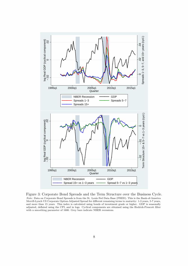
bonds perform relative to treasury bills of identical maturity. A clear counter-cyclicalbehavior is detectable for bonds of all maturities. Table 3 shows a negative correlationbetween output and bond spreads of different maturities.

Term Structure. The lower panel of Figure 3 shows the difference between spreadson long-term bonds (remaining maturity of 5 − 7 years, in green, and more than 15years, in blue) and spreads on bonds of remaining maturity between 1 and 3 years. Thisdifference is called the term structure of bond spreads. The term structure declinesduring downturns as short-term spreads increase faster than long-term spreads. Table 3shows a positive correlation between output and the term structure of corporate bondspreads.


ρxGDP 1.00 1.00 0.46Corporate Value Added 0.95 1.86 0.46Spread 1-3 years -0.53 0.67 0.21Spread 5-7 years -0.56 0.49 0.24Spread 15+ years -0.43 0.35 0.22Difference 15+ vs 1-3 years 0.57 0.36 0.18Difference 5-7 vs 1-3 years 0.39 0.20 0.20

Table 3: Business Cycle Statistics (yearly data)Note: Data on Corporate Bond Spreads is from the St. Louis Fed Data Base (FRED). This is the Bank-of-AmericaMerrill-Lynch US Corporate Option-Adjusted Spread for different remaining terms to maturity: 1-3 years, 5-7 years,and more than 15 years. This index is calculated using bonds of investment grade or higher. GDP and CorporateValue Added are seasonally adjusted, deflated using the CPI, in logs, and de-trended. Cyclical components areobtained using the Hodrick-Prescott filter with a smoothing parameter of 6.25. The second column shows thecorrelation with GDP, the third column shows the relative standard deviation with respect to GDP, the last columnshows the 1st order autocorrelation coefficient.

7

0.0

2.0

4S

prea

ds 1

−3,

5−

7, a

nd 1

5+ y

ears

(cy

cl.)

−.0

20

.02

log

Rea

l GD

P (

cycl

ical

com

pone

nt)

1995q1 2000q1 2005q1 2010q1 2015q1Quarter

NBER Recession GDPSpreads 1−3 Spreads 5−7Spreads 15+

−.0

2−

.01

0T

erm

Str

uctu

re 1

5+ &

5−

7 vs

1−

3 ye

ars

(cyc

l.)

−.0

20

.02

log

Rea

l GD

P (

cycl

ical

com

pone

nt)

1995q1 2000q1 2005q1 2010q1 2015q1Quarter

NBER Recession GDPSpread 15+ vs 1−3 years Spread 5−7 vs 1−3 years

Figure 3: Corporate Bond Spreads and the Term Structure over the Business Cycle.Note: Data on Corporate Bond Spreads is from the St. Louis Fed Data Base (FRED). This is the Bank-of-AmericaMerrill-Lynch US Corporate Option-Adjusted Spread for different remaining terms to maturity: 1-3 years, 5-7 years,and more than 15 years. This index is calculated using bonds of investment grade or higher. GDP is seasonallyadjusted, deflated using the CPI, and in logs. Cyclical components are obtained using the Hodrick-Prescott filterwith a smoothing parameter of 1600. Grey bars indicate NBER recessions.

8

4. Two-period Model

The previous section has established the counter-cyclical behavior of default, bondspreads, leverage, and debt maturity, and the pro-cyclical behavior of the term struc-ture of corporate bond spreads. In this section, we will use a simple two-period setup toderive analytical results on the cyclical properties of default, bond spreads, and lever-age. These cyclical properties will crucially depend on whether the firm has outstandinglong-term debt.

We solve the problem of a firm which finances its capital stock using equity and debt.The optimal capital structure solves a trade-off between the tax advantage of debt andexpected costs of default.

4.1. Setup

There are two periods: t = 0, 1. Consider a firm owned by risk-neutral shareholders.In period 1, the firm can use capital k to produce output y using a technology withdiminishing returns:

y = z f(k) . (1)

The production function f(k) is increasing and concave. We assume that the marginal

product is a constant fraction of its average product: f ′(k) ∝ f(k)k

. To give an example,this property is satisfied by f(k) = kα. Revenue productivity z is known in period 0when capital k is chosen.

Capital depreciates at rate δ. Earnings before interest and taxes are given as:

z f(k)− δk + εk , (2)

where ε is a firm-specific earnings shock. Its value is uncertain at time 0 when capital k ischosen. It follows a probability distribution ϕ(ε) with mean zero and standard deviationσε. Variations in ε capture unforeseen events which directly affect firm earnings.

Markets are exogenously incomplete. There are two ways to finance the capital stockk. The firm can raise funds using equity and debt.

Definition: Debt. A debt security is a promise to pay one unit of the numeraire goodtogether with a fixed coupon payment c at the end of period 1. The quantity of thesebonds is b. Coupon payments cb are fully tax-deductible.

Firm earnings are taxed at rate τ . This implies for shareholders’ net worth afterproduction in period 1:

q = k − b+ (1− τ)[zf(k)− δk + εk − cb] . (3)

When the firm chooses b, there may already be a quantity b of bonds outstanding. Thisis long-term debt which has been issued at some earlier point in time and which maturesat date 1 just like the one-period debt which the firm can sell in period 0. The firm can

9

finance capital in period 0 either using equity or by increasing its debt level b above theinitial stock of long-term debt b through the sale of additional bonds:

k = e+ p(b− b) , (4)

where e is the quantity of equity invested by shareholders in period 0, and p is the marketprice of a bond sold by the firm.

Debt is risky as the firm can decide to default on its liabilities after ε is realized inperiod 1.

Definition: Limited Liability. Whenever the firm’s asset value after production islower than its debt liabilities, full repayment would result in negative net worth q.Shareholders are protected by limited liability. They are free to default and hand overthe firm’s assets to creditors for liquidation. A fixed fraction ξ of the firm’s assets is lostin this case.

Timing

t=0 Given revenue productivity z and an existing stock of debt b, the firm choosescapital k. Capital is financed using equity e and by the revenue p(b− b) from thesale of additional bonds.

t=1 ε is realized. This determines net worth q. The firm decides whether to default.

4.2. Firm Problem

The firm maximizes shareholder value. Limited liability protects shareholders from largenegative realizations of the idiosyncratic earnings shock ε. Given a firm’s stock of capitalk and debt b, there is a unique threshold realization ε which sets shareholders’ net worthequal to zero:

ε : 0 = k − b+ (1− τ)[zf(k)− δk + εk − cb] . (5)

If ε is smaller than ε, shareholders optimally choose to stop paying their liabilities anddefault.

In period 0, the firm decides on its scale of production k, and its preferred capitalstructure consisting of equity e and debt b, in order to maximize expected shareholdervalue at the end of period 1:

maxk,e,b,ε

− e +1

1 + r

∫ ∞ε

[k − b+ (1− τ)[zf(k)− δk + εk − cb] ϕ(ε) dε (6)

subject to: 0 = k − b+ (1− τ)[zf(k)− δk + εk − cb]

k = e+ p (b− b) ,

10

where 11+r

is the shareholders’ discount factor. The bond price p depends on the firm’sbehavior.

4.3. Creditors’ Problem

Creditors are risk-neutral. They discount the future at the same rate 11+r

as shareholders.If shareholders stop paying their liabilities and default, the firm’s asset value is:

q(k, ε) ≡ k + (1− τ)[zf(k)− δk + εk] . (7)

In case of default, creditors liquidate the firm’s assets and receive (1 − ξ)q(k, ε).8 Inperiod 0, the price which they pay for a bond depends on the firm’s characteristics.Creditors break even on expectation:

p(ε, b, k

)=

1

1 + r

[[1− Φ(ε)](1 + c) + Φ(ε)

(1− ξ)q(k, ε)b

]. (8)

Definition: Credit Spreads. For a riskless bond which promises a safe payment of1 + c in period 1, creditors pay a price pr = 1+c

1+r. In case we have c = r, the price of

the riskless bond is 1. The price p of a bond issued by the firm is lower than pr if andonly if the probability of default is positive. In this case, there will be a positive creditspread: 1 + rb − (1 + r) = 1+c

p− (1 + r), where rb is the interest rate which firms pay.

4.4. Equilibrium

We solve for the partial equilibrium allocation given the exogenous and fixed discountrate 1

1+r. In equilibrium, the firm maximizes shareholder value subject to creditors’

break-even condition.9

4.4.1. Consolidated Problem

It is useful to express the stock of debt b in terms of other variables. From the definitionof ε it follows:

b =k + (1− τ)[zf(k)− δk + εk]

1 + (1− τ)c. (9)

8Even a defaulting firm still services εk. The idea is that ε is realized slowly as the firm monitorsits cash flow. Assume that the firm learns about ε by observing a number x with initial value +∞ andwhich subsequently falls towards ε. In this case, the firm optimally services all payments associated toε until ε falls below ε.

9Sometimes more than one bond price satisfies creditors’ zero-profit condition. In this case, differentbond prices imply different default probabilities. By allowing the firm to directly select the defaultprobability through ε, we implicitly assume that the firm sells its bonds to creditors by making a take-it-or-leave-it offer specifying both a price and a quantity of bonds. In this setup, the firm is able toalways select the preferred bond price and the preferred default probability. For the phenomenon ofmultiple bond prices, see Calvo (1988) with an early analysis, Crouzet (2016), or Nicolini, Teles, Ayres,and Navarro (2015) with clarifying results on the role of timing and strategy sets.

11

Shareholders promise a part of the firm’s post-production assets to creditors. Thispromise b[1+(1−τ)c] consists of two parts: the safe part of firm assets after production,k+(1−τ)[zf(k)−δk], and a fixed amount of the risky part of earnings, (1−τ)εk. Fromk = e+ p(b− b), we derive:

e = k − p(b− b) . (10)

The more funds the firm raises on the bond market, the less equity shareholders have toinject. Using these two expressions, the firm’s objective can be re-written as:

− k + p(b− b) +1− τ1 + r

k

∫ ∞ε

[ε− ε] ϕ(ε) dε . (11)

The firm maximizes the total payoff generated from the investment of capital k in thefirm. Since creditors break even on expectation, shareholders appropriate the entiresurplus created by the investment both of equity e and debt p(b− b). Dividends k[ε− ε]are taxed at rate τ . They are positive if ε is higher than the threshold value ε. The bondprice p is a function of k, ε, and b only. This allows us to describe the firm’s problem asa maximization problem in two variables:

maxk,ε

− k +1

1 + r

[[1− Φ(ε)](1 + c) + Φ(ε)

(1− ξ)q(k, ε)b

](b− b)

+1− τ1 + r

k

∫ ∞ε

[ε− ε] ϕ(ε)dε (12)

subject to: b =k + (1− τ)[zf(k)− δk + εk]

1 + (1− τ)c.

The variable k controls the scale of production. The variable ε decides how much of firmearnings (before interest and taxes) are paid out as taxable dividends and how muchis paid to creditors in the form of coupon payments that are fully tax-deductible. Thedownside of raising ε is that costly default becomes more likely.

4.4.2. First Order Conditions

Consider the special case that ξ = 1. A first order condition for an optimal choice of kis:

k : −1 +1− Φ(ε)

1 + r(1 + c)

∂b

∂k+

1− τ1 + r

∫ ∞ε

[ε− ε] ϕ(ε) dε = 0 . (13)

A marginal increase in k has opportunity cost 1. A part of the increase in k is financed bythe sale of additional bonds. If default is avoided, payments to bond holders increase by

(1 + c) ∂b∂k

. This benefit is weighted with the probability that default is avoided 1−Φ(ε).The last term shows that the expected value of dividends grows as the scale of productionis increased. For a given value of ε, the firm’s choice of debt b grows in k according to:

∂b

∂k=

1 + (1− τ)[zf ′(k)− δ + ε]

1 + (1− τ)c. (14)

12

As the scale of production is increased, the value of debt grows less and less becauseof diminishing returns in the safe component of firm earnings. The firm’s objective isstrictly concave in k. The optimal scale of production is uniquely identified.

Note that the effect of an increase in ε on the firm’s choice of k is ambiguous. Theincrease in ε raises the share of firm earnings which are paid out as tax-deductible interestpayments. This reduces the effective marginal tax rate and encourages investment. Thedownside of an increase in ε is that expected default costs rise. This reduces the bondprice and raises the spread. Shareholders have to inject more equity for a given amountof expected dividends. This discourages investment.

A first order condition for an optimal choice of ε is:

ε : [1− Φ(ε)]

[(1 + c)

∂b

∂ε− (1− τ)k

]− ϕ(ε)(1 + c)(b− b) = 0 . (15)

If default is avoided, an increase in ε reduces the expected amount of taxable dividend

payments by (1 − τ)k and increases the payments to bond holders by (1 + c) ∂b∂ε

. Thisraises the share of firm earnings which is exempt from taxation. This benefit is measuredby the term in squared brackets:

(1 + c)∂b

∂ε− (1− τ)k = (1− τ)k

τc

1 + (1− τ)c(16)

This term is always positive. It is linear in k and increasing in the coupon c. The benefitis weighted with the likelihood that default is avoided, 1−Φ(ε). This likelihood is fallingin ε which is captured by the second term of the first order condition (15) above. Givenξ = 1, bond holders lose the full amount of (1+c)b in case of default. Through creditors’break-even condition, the firm internalizes only the part of this loss which is borne bythe buyers of newly issued bonds (1 + c)(b − b). The firm disregards that by sellingadditional bonds it dilutes the value of previously issued bonds. The optimal value of εis pinned down by the trade-off between the tax advantage of debt and the part of theexpected costs of default which is internalized by the firm.

4.4.3. Cyclical Properties

We are interested in how the default rate and the credit spread move over the businesscycle. High values of z create a boom period and low values of z a recession. Throughoutthis section, we assume that the firm’s problem described above has an interior solution.

Proposition 4.1. The default rate and the credit spread are falling in z if and only ifb > 0. Without long-term debt (b = 0), the default rate, the credit spread and leverageare all constant in z.

Proofs can be found in the appendix. A necessary condition for the result that thedefault rate, the credit spread, and leverage are all constant in z if b = 0 is the propertyof f(k) that its marginal product is a constant fraction of its average product. The

13

marginal product f ′(k) appears in the first order condition associated to k, the average

product f(k)k

appears in the first order condition associated to ε. The scale of productionk responds to changes in z but the ratio between the marginal product and the averageproduct remains constant. In the proof we show that this implies that the firm’s choiceof ε is independent of z.

Leverage is given by

b

k=

1 + (1− τ)[z f(k)

k− δ + ε

]1 + (1− τ)c

. (17)

If b = 0, ε is constant in z. The cyclicality of leverage depends on average output percapital z f(k)

k. In the proof we show that the firm optimally adjusts k to keep z f(k)

k

constant.The introduction of long-term debt profoundly affects the cyclical behavior of the de-

fault rate, the credit spread, and leverage in this economy. In the absence of outstandinglong-term debt, changes in aggregate revenue productivity z leave the default rate, thecredit spread, and leverage unaffected. But if the firm inherits some previously issuedlong-term debt, a drop in z increases the default rate and the credit spread.

Compensation Payments. Why does the introduction of long-term debt change thecyclical behavior of the firm? Consider the total value of previously issued bonds:

pb =1− Φ(ε)

1 + rb(1 + c) . (18)

This value decreases if the firm’s current actions cause ε to rise. The firm takes creditors’break-even constraint into account when it chooses k and ε. But only the value of newlyissued bonds b− b enters the firm’s objective. The firm ignores changes in the value ofpreviously issued bonds pb.

To see why this matters for the cyclical behavior of default, consider an alternativescenario in which the firm needs to compensate the owners of previously issued bondsif pb deviates from some reference value M . When the firm chooses equity and debt inperiod 0, it needs to pay a compensation M − pb.10 Subtracting the term M − pb fromthe firm’s objective yields a new maximization problem:

maxk,ε

− k −M +1

1 + r[1− Φ(ε)](1 + c)b +

1

1 + r

∫ ∞ε

(1− τ)k[ε− ε] ϕ(ε)dε

(19)

subject to: b =k + (1− τ)[zf(k)− δk + εk]

1 + (1− τ)c.

Now the firm not only internalizes the value of newly issued bonds b− b, but the valueof the entire stock of debt b, old and new bonds alike. From this problem’s first order

10In models of long-term debt and sovereign default, this method is used by Chatterjee and Eyigungor(2012) and Hatchondo et al. (2016).

14

conditions, we can derive the following result.

Proposition 4.2. If the firm must compensate creditors for changes in the value ofpreviously issued bonds, the default rate, the credit spread, and leverage are all constantin z for any value of b ≥ 0.

It follows from Proposition 4.2 that the result stated in Proposition 4.1 is entirely dueto the fact that the firm does not internalize the effect of its actions on the value of bondsissued in the past. An increase of ε through the sale of additional bonds dilutes the valueof previously issued bonds. Shareholders ignore this effect. They take the increase ofε into account only as far as it reduces the value of newly issed bonds p(b − b). Thisdisregard of a part of the total default costs increases the firm’s choice of ε for any givenvalue of z. Debt dilution raises the default rate at each point of the business cycle.

Cyclical Debt Dilution. Proposition 4.1 states that the default rate is high if z islow if and only if b > 0. So why is it that debt dilution causes the default rate to moveover the business cycle? We know from equation (15) that the benefit of a marginal

increase in ε is proportional to k. The cost is proportional to b− b. If b = 0, leverage bk

is constant in z. This implies that the cost of a marginal increase in ε is proportional tok as well. If b > 0, the firm still enjoys all the benefits of an increase in ε but it ignoresa fraction b

kof the associated costs. If k is large relative to b, this effect is small. But

if k is small relative to b, the firm disregards a larger fraction of the total costs of anincrease in ε and its choice of ε will be higher. Since k is low if z is low and b cannotrespond to changes in z, b

kis high if z is low. Debt dilution causes ε to increase. The

default rate becomes counter-cyclical.

Debt Overhang. From the proofs of Proposition 4.1 and 4.2, an additional resultfollows which characterizes the role of outstanding long-term debt b.

Lemma 4.3. The default rate and the credit spread are increasing in b ≥ 0. If the firmneeds to compensate creditors for changes in the value of previously issued bonds, thedefault rate, the credit spread, and leverage are all constant in b ≥ 0.

The intuition for this result is clear. The higher the fraction of the total potentialcosts of default which the firm disregards, the higher is the firm’s choice of ε. Once thefirm is forced to internalize the effect of its actions on the value of outstanding long-term debt, this mechanism is absent. Gomes et al. (2016) find a closely related result.Just like in our model, firms are restricted to time-consistent policies. A negative shockto inflation increases the real value of outstanding long-term debt. Firms respond bychoosing higher leverage and a higher risk of default. Leverage and default risk remainelevated until the real value of outstanding long-term debt has returned to its long-runmean. Viewed through the lens of our model, this phenomenon of “sticky leverage” canbe understood as a manifestation of debt dilution. With nominal debt, a drop in theprice level corresponds to a persistent increase of b in our model. Lemma 4.3 states thatin the presence of debt dilution the default rate is an increasing function of b.

15

5. Dynamic Model

Now that we have studied the cyclical role of debt dilution in a two-period economy, weuse these results to understand debt dilution in a fully dynamic model with a maturitychoice. Firms can choose between selling short-term bonds and long-term bonds. Long-term debt is unattractive because it gives rise to debt dilution in the future. Short-termdebt has the disadvantage that its entire amount needs to be rolled-over each period.This is costly because of a transaction cost on the bond market.

5.1. Setup

There is a unit mass of firms. As in the two-period economy, a firm i uses capital kit toproduce output yit using a technology with diminishing returns:

yit = zt kαit , α ∈ (0, 1) . (20)

Earnings before interest and taxes are given as:

zt kαit − δkit + εitkit . (21)

The firm-specific earnings shock εit is i.i.d. and follows a probability distribution ϕ(ε)with mean zero and standard deviation σε.

In contrast to the two-period economy, the firm can now choose between two debtinstruments of different maturity. Short-term debt and long-term debt are of equalseniority.

Definition: Short-term Debt. A short-term bond issued at the end of period t is apromise to pay one unit of the numeraire good together with a fixed coupon payment cin period t+ 1. The quantity of short-term bonds sold by firm i is bSit.

Definition: Long-term Debt. A long-term bond issued at the end of period t is apromise to pay a fixed coupon payment c in period t + 1. In addition, the firm repaysa fraction γ of the principal. In period t + 2, a fraction 1 − γ of the bond remainsoutstanding. Creditors receive a coupon payment (1− γ)c. In addition, the firm repaysa fraction of the remaining principal: (1− γ)γ. In this manner, payments geometricallydecay over time. The maturity parameter γ controls the speed of decay. The quantityof long-term bonds is bLit.

This computationally highly tractable specification of long-term debt goes back toLeland (1994).11

11The Macaulay duration µ of this long-term bond is:

µ =1

pLr

∞∑j=1

j (1− γ)j−1c+ γ

(1 + r)j=

c+ γ

pLr

1 + r

(γ + r)2, (22)

16

Definition: Transaction cost. The firm pays an amount η for each unit of short-termbonds sold and each unit of long-term bonds sold or repurchased:

H(bSit, bLit, b

Lit) = η(bSit + |bLit − bLit|) , (25)

where bLit is the stock of outstanding long-term bonds.

Firm net worth after production is:

qit = kit − bSit − γbLit + (1− τ)[ztkαit − δkit + εitkit − c(bSit + bLit)] . (26)

The firm raises capital by injecting equity and from selling short- and long-term bonds:

kit = eit + pSitbSit + pLit(b

Lit − bLit)−H(bSit, b

Lit, b

Lit) . (27)

Dividends are given bydit = qit − eit+1 . (28)

Definition: Limited Liability. Shareholders are protected by limited liability. Theyare free to default and hand over the firm’s assets to creditors for liquidation. A fixedfraction ξ of the firm’s assets is lost in this case. After default, shareholders are free tostart a new business with zero equity and zero debt.

Timing

End of period t− 1: Aggregate revenue productivity zt is realized. Firm i has anamount bLit of long-term debt outstanding. Given zt and bLit, the firm choosesnext period’s book value of equity eit. It also decides how to adjust its level oflong-term debt bLit and how many short-term bonds bSit to sell. This determinesnext period’s stock of capital kit.

Beginning of period t: The firm draws the realization εit. This determines firm earn-ings. The firm decides whether to default. If it decides not to default, it payscorporate income tax on earnings net of depreciation and coupon payments. Thisleaves the firm with net worth qit. Next period’s amount of long-term debt isbLit+1 = (1− γ)bLit.

where pLr is the price of a riskless long-term bond:

pLr =

∞∑j=1

(1− γ)j−1c+ γ

(1 + r)j=c+ γ

r + γ. (23)

It follows for the Macaulay duration:

µ =1 + r

γ + r. (24)

17

5.2. Firm Problem

The firm maximizes shareholder value. As in the two-period economy, there is a uniquethreshold realization εit which decides whether shareholders prefer to default:

εit : kit − bSit − γbLit + (1− τ)[ztkαit − δkit + εitkit − c(bSit + bLit)]

+ Ezt+1|zt V(

(1− γ)bLit , zt+1

)= Ezt+1|zt V

(0 , zt+1

), (29)

where V (bLit+1, zt+1) denotes the end-of-period-t stock market value of a firm with long-term debt bLit+1 when aggregate revenue productivity is zt+1. If εit turns out to be smallerthan εit, shareholders optimally choose to stop paying their liabilities and default.

We assume that the firm has no ability to commit to future actions. The firm under-stands the decision problem it will face at future points in time. It must take its ownfuture behavior as given when deciding about its policy today. We restrict attention tostrategies which are functions of the current state of the firm. That is, we are study-ing the Markov Perfect equilibrium of the game which the firm plays against its futureselves.

The firm maximizes the discounted sum of future dividend payments. For ease ofexposition, we drop firm- and time-subscripts from now on. The state of the firm iss = (b, z). The firm chooses a policy vector φ(s) = (k, e′, bS, bL, ε) as a solution to theproblem

V (b, z) = maxk,e′,bS ,bL,ε

− e′ + 1

1 + r

[ ∫ ∞ε

[q′ + Ez′|zV ((1− γ)bL, z′)

]ϕ(ε)dε

+ Φ(ε)Ez′|z V (0, z′)

](30)

subject to: q′ = k − bS − γbL + (1− τ)[zkα − δk + εk − c(bS + bL)]

ε : q′ + Ez′|zV ((1− γ)bL , z′) = Ez′|zV (0 , z′)

k = e′ + pS bS + pL(bL − b)−H(bS, bL, b) .

The two bond prices pS and pL depend on the firm’s behavior.

5.3. Creditors’ Problem

Once the firm stops paying its liabilities and defaults, the value of the firm’s assets is

q(k, ε, z) ≡ k + (1− τ)[zkα − δk + εk] . (31)

At this point, creditors liquidate the firm’s assets and receive (1− ξ)q(k, ε, z). There aretwo bond prices: pS and pL. On expectation, risk-neutral creditors’ break even on both

18

types of bonds:

pS(s, φ(s)

)=

1

1 + r

[[1− Φ(ε)] (1 + c) + Φ(ε)

(1− ξ)q(s, φ(s)

)bS + bL

], and (32)

pL(s, φ(s)

)=

1

1 + r

[[1− Φ(ε)]

(γ + c+ (1− γ)Ez′|z pL

(s′, φ(s′)

) )+ Φ(ε)

(1− ξ)q(s, φ(s)

)bS + bL

]. (33)

Definition: Credit Spreads. As in the two-period economy, the spread on short-termbonds is:

1 + rS − (1 + r) =1 + c

pS− (1 + r) . (34)

Assuming a constant price pL, the return on risky long-term bonds is:

1 + rL =c+ γ + (1− γ)pL

pL=c+ γ

pL+ 1− γ . (35)

It follows for the long-term spread:

1 + rL − (1 + r) =c+ γ

pL+ 1− γ − (1 + r) . (36)

5.4. Equilibrium

As in the two-period economy, we solve for the partial equilibrium allocation given theexogenous and fixed discount rate 1

1+r. In equilibrium, firms maximize shareholder value

subject to creditors’ two break-even conditions.

Recursive Markov Equilibrium. A recursive equilibrium for this economy is (i) a setof policy functions for capital k(b, z), equity e′(b, z), short-term debt bS(b, z), long-termdebt bL(b, z), and a default threshold ε(b, z), and (ii) price functions for short-term debtpS(k, bS, bL, ε, z) and long-term debt pL(k, bS, bL, ε, z), such that the following conditionshold:

1. Taking the bond price functions pS(k, bS, bL, ε, z) and pL(k, bS, bL, ε, z) as given,the policy functions k(b, z), e′(b, z), bS(b, z), bL(b, z), and ε(b, z) solve the firmproblem (30).

2. The bond price functions pS(k, bS, bL, ε, z) and pL(k, bS, bL, ε, z) satisfy creditors’break-even conditions (32) and (33).

There is a time-inconsistency problem which enters through the price of long-termdebt pL

(s, φ(s)

). Through next period’s price pL

(s′, φ(s′)

), this price depends on the

firm’s behavior in the future. Creditors anticipate future debt dilution. This depressestoday’s price of long-term debt. The firm would like to commit to internalize all future

19

expected costs of default on bonds issued today. This would raise the bond price todayand increase shareholder value. From the point of view of the firm today, the futurepolicy φ(s′) is not chosen optimally. Lack of commitment means that the only way inwhich the firm can limit debt dilution is through the future state variable (1− γ)bL.

Firms differ with respect to the amount of long-term debt outstanding. Some firmshave defaulted in the past and started anew with zero debt. Given a distribution of firmsover long-term debt outstanding b, aggregate variables are constructed as a weightedaverage of firm policies.

5.4.1. Consolidated Problem

As in the two-period economy, it is useful to simplify the problem. The consolidatedproblem will allow us to numerically compute equilibrium bond prices and firm policiesin a single step. We define the share of long-term debt as

m =bL

bS + bL. (37)

Given m we can back out the amount of short-term bonds:

bS =1−mm

bL . (38)

Using the definition of ε, the value of bL can be expressed as:

bL = G(k, ε,m, z) . (39)

From k = e′ + pS bS + pL(bL − b)−H(bS, bL, b), we derive:

e′ = k − pS bS − pL(bL − b) +H(bS, bL, b) . (40)

The firm objective becomes

− k + pS bS + pL(bL − b)−H(bS, bL, b)

+1

1 + r

[ ∫ ∞ε

[k − bS − γbL + (1− τ)[zkα − δk + εk − c(bS + bL)]

+ Ez′|zV ((1− γ)bL, z′)]ϕ(ε)dε + Φ(ε)Ez′|z V (0, z′)

]. (41)

We have expressed bS and bL as functions of the choice variables k, ε, m, and the ag-gregate state z. Using creditors’ zero-profit condition, this allows us to pin down theshort-term bond price pS(s, φ(s)) as a function of the same three choice variables andthe aggregate state. Similarly, the long-term bond price pL(s, φ(s)) can be expressed asa function of k, ε, m, z, together with tomorrow’s price pL(s′, φ(s′)). Given tomorrow’sprice function of long-term debt pL(s′, φ(s′)) and a probability distribution for the ex-

20

ogenous state z, both bond prices pS(s, φ(s)) and pL(s, φ(s)) are pinned down by thefirm’s choice of k, ε, and m.

The firm’s problem is simply to choose values for k, ε, and m which maximize itsobjective function (41) taking as given tomorrow’s price function for long-term debtpL(s′, φ(s′)) and the firm’s value function V (b′, z′). The solution to this consolidatedproblem computes the equilibrium bond prices, pS(s, φ(s)) and pL(s, φ(s)), and today’sfirm policy, k, ε, m, in a single step.

5.5. Quantitative Analysis

The firm’s choice between short-term and long-term debt can only be studied in a fullydynamic economy. That is why we turn to a quantitative analysis.

5.5.1. Solution Method

We solve the model numerically using value function iteration and interpolation. Wefollow the literature on sovereign default with long-term debt in that we solve for theequilibrium allocation of a finite-horizon economy. Starting from the final date, weiterate backward in time until the firm’s value function and the two bond prices haveconverged. We then use the first-period equilibrium functions as the infinite-horizon-economy equilibrium functions.12

Common practice in the literature on long-term debt is to compute the complete bondprice schedules for all possible states and actions: pS(k, bS, bL, ε, z) and pL(k, bS, bL, ε, z).These price schedules are then used to compute the optimal policy. In Section 5.4.1 wehave re-formulated the firm problem in a way which expresses equilibrium bond pricesas a function of today’s choice variables. Given the firm’s future policy and a probabilitydistribution for the exogenous state z, both bond prices are pinned down by the firm’schoices today. This allows us to use the consolidated problem to compute equilibriumbond prices and today’s firm policy in a single step. This reduces the number of necessarycomputations and allows for a faster and more precise solution.

5.5.2. Parametrization

We choose parameter values in order to replicate a number of key statistics from the U.S.for the time period 1984 - 2015, presented in Table 4. In the data, short-term liabilitieshave term to maturity of up to one year. We therefore choose the model period to beone year. Model counterparts of targeted empirical moments are summarized in Table5. If c = r, the price of a riskless short-term bond and a riskless long-term bond in ourmodel are both equal to one.

A key parameter in the model is γ. This parameter controls the speed of decay inpayments on the long-term bond. We choose its value to match the average Macaulayduration of 6.5 years reported by Gilchrist and Zakrajsek (2012) for a sample of 5,982

12This solution method is used for instance by Hatchondo and Martinez (2009).

21

senior unsecured bonds issued by U.S. non-financial firms. Table 6 reports our choicefor the full set of parameter values.

Mean1984-2012:Default Rate (yearly) 0.72%1984-2015:Leverage: Liabilities / Assets 45.7%Long-term Liabilities Share 67.1%1973-2010:Macaulay Duration 6.5 years1997-2015:Spread 1-3 years 1.32%Spread 3-5 years 1.46%Spread 5-7 years 1.69%Spread 7-10 years 1.70%Spread 10-15 years 1.71%Spread 15 years and more 1.82%

Table 4: Empirical MomentsNote: Default rates are from Giesecke et al. (2014). This is the ratio of ’total par value of outstanding non-financialcorporate bonds which are in default’ over ’total par value of outstanding non-financial corporate bonds’. TotalAssets, Short-term Liabilities, and Total Liabilities of non-financial corporate firms are from the Flow of Funds.Duration is from Gilchrist and Zakrajsek (2012). Data on Corporate Bond Spreads is from the St. Louis Fed DataBase (FRED). This is the Bank-of-America Merrill-Lynch US Corporate Option-Adjusted Spread using bonds ofinvestment grade or higher.

Aggregate revenue productivity zt follows an AR(1)-process:

zt = ρzt−1 + εz , (42)

where εz is white noise with standard deviation σz. The firm-specific earnings shock isNormal with zero mean and standard deviation σε. We choose values for ρ and σz inorder to generate an empirically plausible time path of GDP.13

We set the yearly rate of return on a riskless asset to r = 3.09%. The parameter valuesof α and τ are taken from Covas and Den Haan (2012). The parameter δ is meant toaccount for several types of costs which are absent from out model, e.g. wages. Ourchoice generates a mean capital-output ratio of about 2.4.

The values of ξ, η, and σε are chosen to match three empirical moments: leverage,the share of long-term liabilities, and bond spreads. We use two untargeted momentsto verify that our model generates reasonable statistics. The first one is the averagecompensation paid to investment banks for bond placements. Altınkılıc and Hansen

13Using yearly Flow of Funds data from 1984-2015, we estimate an AR(1) process for the detrendedlog real GDP. We use the Hodrick-Prescott filter with a smoothing parameter of 6.25 as recommended byRavn and Uhlig (2002) for yearly data. Our estimates yield an AR(1) coefficient of 0.41 with standarddeviation in the error term of 0.01. Our parametrization targets these estimates.

22

Default Rate Φ(ε)

Total Liabilities D ≡ 1+c1+r

bS + γ+cγ+r

bL

Leverage: Liabilities / Assets Dk

Long-term Liabilities Share 1D

γ+cγ+r

bL

Macaulay Duration 1+rγ+r

Short-term Spread 1+cpS− (1 + r)

Long-term Spread c+γpL

+ 1− γ − (1 + r)

Term Structure c+γpL

+ 1− γ − 1+cpS

Table 5: Key Variables

(2000) report this value to be 1.09% of the proceeds. The corresponding value in ourparametrized model is remarkably close: 0.84%. This suggests that our parameter choicefor the transaction cost on the bond market η is reasonable. The second untargetedmoment is the debt recovery rate in bankruptcy. On average, our parametrized modelgenerates a recovery rate (1 − ξ)q[bS + bL]−1 of 54%. This is broadly in line with theempirical evidence provided by Bris, Welch, and Zhu (2006) who document a meanrecovery rate of 69% for Chapter 11 re-organizations and 27% for Chapter 7 liquidations.

It is well known that empirical bond spreads are not fully explained by realized defaultrisk.14 In our model, bonds spreads are driven exclusively by default risk. This meansthat we have to decide whether we want our model to match the default rate andgenerate unrealistically low bond spreads, or if want to match bond spreads at the costof generating unrealistically high default rates. In our model, the bond price schedule iskey to understanding firm behavior. We therefore choose to match bond spreads ratherthan the default rate.

r 0.0309 γ 0.1277 ξ 0.45 σz 0.0035α 0.7 c r η 0.0082 σε 0.525δ 0.25 τ 0.296 ρ 0.77

Table 6: Parametrization

14See for instance Elton, Gruber, Agrawal, and Mann (2001).

23

5.5.3. Cyclical Properties

We now present numerical results on the response of real and financial variables toinnovations in aggregate revenue productivity z. We focus on the model’s ability togenerate the counter-cyclical behavior of default rates, bond spreads, leverage, and debtmaturity, as well as the pro-cyclical term structure of bond spreads.

Policy Functions. Figures 4 and 5 show firms’ equilibrium policies as functions ofthe exogenous state z and the stock of outstanding long-term debt b. We see that theanalytical results from Proposition 4.1 and 4.3 continue to hold in the fully dynamiceconomy: As the upper four panels of Figure 5 show, the default rate, leverage, andbond spreads are all constant in z as long as b = 0. For positive levels of outstandingdebt, the default rate, leverage, and bond spreads are falling in z. All four variables areincreasing in b. The analytical results from Section 4 allow us to attribute these resultsto debt dilution.15

In Figure 4, we see that firms choose higher values of capital k and output y if z ishigh. This is because the expected marginal return on capital is increasing in z. Alsonote that these variables are falling in b. As the default rate is increasing in b (becauseof debt dilution), the expected return on capital is falling.

If the stock of outstanding long-term debt is high, the firm will choose high levelsof both short-term and long-term debt. In the words of Gomes et al. (2016), debt is“sticky”. This result is due to debt dilution. As b increases, the fraction of the totalpotential costs of default which is internalized by the firm falls. The firm’s response is toaccept a higher risk of default which translates into higher leverage. The dashed line inthe middle panel on the right side of Figure 4 indicates stable points for long-term debt.In our parametrization, the stable choice of long-term debt bL for non-defaulting firmslies around 5.6 which, given our choice of γ = 0.1277, implies a corresponding value foroutstanding long-term debt b = (1− γ)bL of around 4.9.

The way equity e′ responds to a higher level of b depends on the relative strength oftwo forces. On the one hand, higher values of b and higher credit spreads push towardsa higher value of e′ for given values of k and debt. On the other hand, the fact thatboth short-term debt and long-term debt are increasing in b and that capital k is fallingpushes in the opposite direction. Figure 4 shows the resulting equilibrium outcome.Equity is increasing for low values of b and falling for higher values of b.

Shareholder value (i.e. the firm’s value function) is increasing in z and falling in b.If b is high, a large part of the total firm value has been promised to the holders ofpreviously issued long-term debt and only a small part is left for shareholders.

The left panel in the bottom row of Figure 5 shows the term structure of bond spreads:the difference between the long-term and short-term bond spreads. For low values of b,creditors expect that the firm will increase the amount of long-term debt in the future.

15If we had not allowed firms to issue long-term debt, the default rate, leverage, and bond spreadswould all be perfectly a-cyclical. In Appendix B.2 we show firms’ equilibrium policies when only short-term debt is available.

24

Long-term Debt outstanding0 2 4 6

Cap

ital

12

14

16

18

Capital policy

low z

medium z

high z


Equ

ity

12

14

16

18

Equity policy


Sho

rt-t

erm

Deb

t

0

2

4

6

8Short-term Debt policy


Long

-ter

m D

ebt

0

2

4

6

8Long-term Debt policy


Out

put

6.5

7

7.5

8Output


Sha

reho

lder

Val

ue

44

46

48

50

52

54Value Function

Figure 4: Policy Functions Part I.

25


Def

ault

rate

0

0.02

0.04

0.06

0.08

0.1Default rate

low z

medium z

high z


Leve

rage

0

0.2

0.4

0.6

0.8Leverage


Sho

rt-t

erm

Bon

d S

prea

d

0

0.01

0.02

0.03

0.04

0.05Short-term Bond Spread


Long

-ter

m B

ond

Spr

ead

0

0.01

0.02

0.03

0.04

0.05Long-term Bond Spread

Long-term Debt outstanding0 2 4 6T

erm

Str

uctu

re o

f Bon

d S

prea

ds

-0.02

-0.01

0

0.01Term Structure of Bond Spreads


Sha

re o

f Lon

g-te

rm L

iabi

litie

s

0.4

0.5

0.6

0.7

0.8Share of Long-term Liabilities

Figure 5: Policy Functions Part II.

26

Because of debt dilution, this will increase the risk of default. This affects the long-term bond more than the short-term bond, hence the term structure is positive for lowvalues of b. If b is very high, creditors expect that the firm will lower the amount oflong-term debt in the future. This will reduce the extent of future debt dilution. Again,this future reduction in default risk affects the long-term bond much more than theshort-term bond. For this reason, the term structure is negative for high values of b.

Because of cyclical debt dilution, temporarily high values of z decrease the risk ofdefault today. This strongly affects the short-term bond spread which depends exclu-sively on the risk of default today. The long-term bond spread depends on the risk ofdefault in all future periods. Because of mean reversion, the long-term spread is muchless affected by a temporary decline in the risk of default than the short-term spread.Therefore the short-term spread falls more strongly in z and the difference between thelong-term spread and the short-term spread increases in z.

The right panel in bottom third row of Figure 5 shows that the firm’s share of long-term debt is an increasing function of b. Evidently, the firm’s time-inconsistency problemalso affects its maturity choice. For a given amount of total debt, an increase in thelong-term debt share reduces the amount of debt which needs to be rolled over eachperiod. Because of the transaction cost on the bond market, this is beneficial. The costof an increase in the long-term debt share is that debt dilution becomes more severe inthe future. Part of this cost is internalized by the firm through a fall in the long-termbond price today. But another part of this cost is borne by the holders of outstandinglong-term debt. The firm disregards this part. As a result, the firm chooses a higherlong-term debt share if b is high.

Just like the default rate, leverage, and bond spreads, the long-term debt share isfalling in z. The underlying mechanism is identical. As z is increasing, the ratio ofnewly issued debt to outstanding debt increases as well. This raises the share of thetotal value of debt which is internalized by the firm. The firm benefits more from afuture reduction in debt dilution and therefore chooses to reduce the long-term debtshare.

Firm Distribution. At each point in time, the population of firms is heterogeneouswith respect to the amount of long-term debt outstanding b. Figure 6 shows three firmdistributions. For three different levels of z, we plot the distribution which arises follow-ing a long sequence of identical realizations of z. For each given value of z, the majorityof firms has not defaulted for a long time. These firms eventually find themselves nearthe stable values for outstanding long-term debt of around 4.9. Firms always choose apositive risk of default. A firm which defaulted continues to operate with b = 0. Debtdilution is not a concern for this firm. For this reason, the firm initially chooses lowvalues of bL. But with a positive amount of long-term debt outstanding, debt dilutioninduces the firm to take on more and more long-term debt over time, until the firmreaches a stable value.

27

Long-term Debt outstanding0 0.5 1 1.5 2 2.5 3 3.5 4 4.5 5 5.5

Pro

babi

lity

mas

s

0

0.1

0.2

0.3

0.4

0.5

0.6Firm Distributions

low zmedium zhigh z

Figure 6: Firm Distributions.

Impulse Response Functions. The impulse response functions shown in Figure 7confirm our observations from studying firms’ equilibrium policy. We study the responseof aggregate variables to a one-time drop in z. Aggregate variables are constructed asa weighted average of firm policies using the time-varying firm distribution over b. Thisdistribution does not play an interesting role in this model economy. In the aggregate,leverage, the default rate, bond spreads, and the long-term debt share are all somewhatlower than for the median firm which finds itself close to the stable value of b. Apartfrom that, impulse response functions of the median firm are qualitatively identical toimpulse response functions of aggregate variables.

Because of cyclical debt dilution, the default rate, leverage, bond spreads, and thelong-term debt share all increase after a negative shock to aggregate revenue productivityz. Short-term spreads are more volatile than long-term spreads. For this reason, theterm structure of bond spreads falls together with z. Debt dilution is crucial to replicatethese empirical facts in this model economy. If only short-term debt was available, thedefault rate, leverage, and bond spreads would all be perfectly flat over the businesscycle.16

Note that the unconditional level of long-term spreads is slightly below the level ofshort-term spreads. In case of default, short-term creditors lose a promised payment of

16In Appendix B.2 we show impulse response functions for an alternative economy where only short-term debt is available to firms.

28

1020

300.

99

0.99

51Z

1020

30

0.981

Ou

tpu

t

1020

30

0.981

Cap

ital

1020

30

0.981

Eq

uit

y

1020

30

0.981

Sh

ort

-ter

m D

ebt

1020

30

0.981

Lo

ng

-ter

m D

ebt

1020

300.

42

0.43

0.44

Lev

erag

e

1020

300.

66

0.66

5

0.67L

on

g-t

erm

Deb

t S

har

e

1020

302.

93

3.1

Def

ault

Rat

e in

%

1020

300.

015

0.01

55

0.01

6Sh

ort

-ter

m S

pre

ad

1020

300.

015

0.01

55

0.01

6Lo

ng

-ter

m S

pre

ad

1020

30-0

.001

0

-0.0

0050

Ter

m S

tru

ctu

re

Figure 7: Impulse Response Functions.

29

1 + c. Long-term creditors lose γ + c in addition to future payments of value (1− γ)pL.Since the equilibrium price of risky long-term debt pL is smaller than 1, long-termcreditors lose less than short-term creditors. However, both of them are entitled to anidentical claim on the liquidation value of the firm’s assets (1 − ξ)q. For this reason,long-term creditors demand a smaller average spread in our model than short-termcreditors.17

5 10 15 20 25 300.992

0.994

0.996

0.998

1Z

5 10 15 20 25 300.97

0.98

0.99

1Output

FrictionlessFinancial Frictions

5 10 15 20 25 300.97

0.98

0.99

1Capital

FrictionlessFinancial Frictions

Figure 8: Amplification through Cyclical Debt Dilution.

Amplification. Figure 8 compares three of the impulse response function from Figure7 with a model of frictionless capital markets and zero taxation. The first best level ofcapital is described by the following first order condition:

zαkα−1fl − δ − r = 0 ⇔ kfl =

(zα

δ + r

) 11−α

. (43)

The responses of output and capital in our benchmark economy are slightly morepronounced than in the frictionless case. In response to the negative shock to z, output

17This preferential treatment of long-term bonds also influences firms’ maturity choice. In ourparametrization, the quantitative significance of this channel turns out to be small. Without thetransaction cost on the bond market (η = 0), firms barely issue any long-term debt.

30

falls by 2.7% compared to 2.55% in the frictionless model. This implies an amplificationof about 5%.18

Cyclical debt dilution causes credit spreads to increase during a downturn. Risingspreads feed back into low investment and less borrowing. This increases the ratio ofpreviously issued debt to newly issued debt further, making debt dilution even moreattractive. Cyclical debt dilution is a potentially powerful feedback loop between lowinvestment and high credit spreads. Given our choice of parameter values, we findits quantitative significance in amplifying firms’ response to fundamental shocks to bemoderate. Different parametrizations, which generate a higher average rate of default,also generate stronger amplification.

5.5.4. Policy Exercises

Long-term debt allows firms to save transaction costs on the bond market, but it alsocreates a time-inconsistency problem. In order to understand the associated costs, weconsider two policy experiments. First we study an outright ban of long-term debt. Sec-ond, we quantify the costs of debt dilution by comparing the results from our benchmarkeconomy to an alternative economy in which long-term bond contracts feature a debtcovenant which completely neutralizes debt dilution. We also refer to empirical evidenceindicating that similar debt covenants are not used in practice.

Throughout this section, we continue to study a model economy with aggregate shocksto z. But for illustrative purposes, we assume that during our policy experiments theexogenous state z happens to stay at its unconditional mean. As a welfare criterion, weuse the surplus created in the corporate sector:

W =

∫ 1

0

[ y(i)− δk(i)− rk(i) ] di , (44)

where y(i) and k(i) are firm i’s choices of output and capital. This welfare criterionimplicitly assumes that taxes, earnings shocks, bankruptcy costs, and the transactioncost on the bond market are all purely redistributive and are not a cost to society asa whole. We interpret the transaction cost on the bond market as a fee charged byinvestment banks for their services. Similarly, some part of bankruptcy costs consists ofpayments to lawyers and auditors. According to our welfare criterion, financial frictionsmatter only insofar as they distort the allocation of capital.19 To the extent that thereare real social costs of bankruptcy, our welfare criterion provides a lower bound forthe efficiency gap with respect to the first best economy without taxation and withfrictionless capital markets.

18If firms are restricted to using only short-term debt as in Appendix B.2, there is no discernibledifference between impulse response functions with and without financial frictions.

19We ignore the fact that lawyers and investment bankers could pursue different valuable activitiesin a first best economy.

31

5010

015

020

00

0.51

1.52

Z

5010

015

020

0

-100-9

0

-80

-70

Ou

tpu

t G

ap in

%

5010

015

020

0

-100-9

0

-80

-70

Cap

ital

Gap

in %

5010

015

020

0

-100-9

0

-80

-70

Wel

fare

Gap

in %

5010

015

020

01415161718

Eq

uit

y

5010

015

020

00510

Deb

t

Long

-ter

m D

ebt

Sho

rt-t

erm

Deb

t

5010

015

020

00

0.1

0.2

0.3

0.4

Lev

erag

e

5010

015

020

00

0.51

Lo

ng

-ter

m D

ebt

Sh

are

5010

015

020

00123

Def

ault

Rat

e in

%

5010

015

020

00

0.00

5

0.01

0.01

5

0.02

Sh

ort

-ter

m S

pre

ad

5010

015

020

00

0.00

5

0.01

0.01

5

0.02

Lo

ng

-ter

m S

pre

ad

5010

015

020

01.

081.1

1.12

1.14

Ret

urn

on

Eq

uit

y

Figure 9: Ban of Long-term Debt.

32

Policy 1: Ban of Long-term Debt

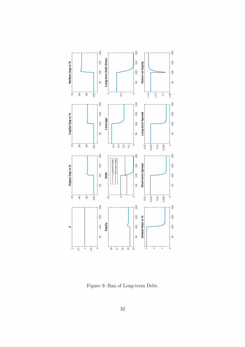
A somewhat extreme policy experiment is an outright ban of long-term debt. In themodel, we consider a constraint which forces firms to set bL = b from time tp onwards.This constraint implies that firms continue to service outstanding long-term bonds, butthey are unable to issue new ones. Over time, firms’ stock of long-term debt convergestowards zero. Up to time tp, the ban of long-term is completely unexpected.

Figure 9 shows what happens in our model economy after the policy intervention attime tp = 100. In the first period after the policy intervention, the default rate, leverage,and bond spreads fall only mildly. The reason is that initially the stock of long-termdebt is still high. Debt dilution is still a concern. The firm makes up for the forcedreduction in long-term debt by sharply increasing its stock of short-term debt. As thestock of long-term debt is gradually reduced, debt dilution becomes weaker. The defaultrate, leverage, and bond spreads all fall and converge to a lower level. The long-run levelof the default rate is about 0.6% compared to almost 3% before the policy intervention.Leverage falls from 43% to 18.5%, credit spreads from 1.5% to 0.3%.

In the first row of Figure 9, we compare our benchmark economy with the first bestallocation. In the first best economy with frictionless capital markets and zero taxes,the allocation of capital is undistorted. Output, capital, and welfare are all higher thanin our benchmark economy. For each period, we calculate the gap in output, capital,and welfare between the two economies. This gap is always positive. We normalize it to100% prior to the policy and track its evolution in response to the policy interventionin period tp.

Output, capital, and welfare all increase in response to the ban of long-term debt.There are two opposing effects at work. As leverage is falling, the effective tax rateon capital increases. This lowers the marginal return on capital. On the other hand,long-term debt gradually disappears following the policy change. Firms respond byreducing leverage. This allows creditors to charge lower short-term bond spreads, ren-dering investment more profitable for firms. This benefit outweighs the higher taxation.The policy intervention reduces the welfare gap with respect to the first best allocationwithout taxation and with frictionless capital markets by 16.8%.

The last panel of Figure 9 shows the return on equity: 1e′

∫∞εq′ϕ(ε)dε. With decreasing

returns in production, firm profits are positive. While creditors break even, shareholdersearn an excess return over the riskless rate. The return on equity falls on impact intp = 100. As the long-term debt share is falling, transaction costs on the bond marketincrease. This effect is strongest right after tp when leverage is still high. Shareholderspay these transaction costs through an increase of book equity e′. This reduces thereturn on equity. But this initial drop is followed by a fast rebound. As leverage falls,the initial increase of transaction costs on the bond market and the associated increasein e′ are partially reversed. And with a lower stock of outstanding long-term debt, thefirm internalizes a larger fraction of the total benefit of reduced debt dilution in the formof lower bond spreads.

33

Policy 2: Measuring the Cost of Debt Dilution

We have seen that an outright ban of long-term debt improves the allocation of capi-tal and increases welfare in our model economy. But given that long-term debt savestransaction costs on the bond market, there might be better ways to address firms’time-inconsistency problem. We conduct a second policy experiment to measure themaximum welfare gain which could be achieved by a complete neutralization of debtdilution. We compare the results from our benchmark economy with long-term debtand debt dilution to an alternative economy in which long-term debt is used but debtdilution is absent. In this alternative economy, firms are obliged to compensate credi-tors for all fluctuations in the value of outstanding long-term bonds which are causedby future borrowing. As we have seen in Section 4, this forces firms to internalize thevalue of outstanding long-term debt.20

In order to know the correct compensation payment, the first step is to calculate thevalue of outstanding long-term debt in the absence of additional borrowing by the firm.Consider the following problem:

V (b, z) = maxk,ε

− k +1

1 + r

[ ∫ ∞ε

[q′ + Ez′|zV ((1− γ)b, z′)

]ϕ(ε)dε

+ Φ(ε)Ez′|z V (0, z′)

](45)

subject to: q′ = k − γb+ (1− τ)[zkα − δk + εk − cb]

ε : q′ + Ez′|zV ((1− γ)b , z′) = Ez′|zV (0 , z′) .

This is the problem of a firm which inherits an amount b of long-term debt from the past,but which is not allowed to sell or buy any bonds, neither short-term bonds nor long-term bonds. Capital is entirely financed by equity: k = e′. As in the model economiesabove, creditors pay a break-even price pL for a long-term bond of this firm. This pricepL is the reference price which we use to compute the correct compensation payment tothe holders of outstanding long-term bonds.

After we have solved problem (45) and calculated the reference price pL, we canstudy the problem of a firm in our alternative economy in which firms must compensatecreditors for all fluctuations in the value of outstanding long-term bonds which are causedby future borrowing. As in our benchmark economy, firms finance capital through equity,short-term debt, and long-term debt. But now long-term bonds feature a covenant whichspecifies a compensation payment from the firm to the holders of long-term debt. Thiscompensation payment depends on the difference between the reference price of long-term bonds pL and the actual price ˆpL. It is equal to: (pL − ˆpL)b. The firm’s problem

20In models of sovereign default and long-term debt, similar compensation payments are consideredby Chatterjee and Eyigungor (2012) and Hatchondo et al. (2016).

34

is given by

ˆV (b, z) = max

k,e′,bS ,bL,ε− e′ + 1

1 + r

[ ∫ ∞ε

[q′ + Ez′|z

ˆV ((1− γ)bL, z′)

]ϕ(ε)dε

+ Φ(ε)Ez′|zˆV (0, z′)

](46)

subject to: q′ = k − bS − γbL + (1− τ)[zkα − δk + εk − c(bS + bL)]

ε : q′ + Ez′|zˆV ((1− γ)bL , z′) = Ez′|z

ˆV (0 , z′)

k = e′ + pS bS + ˆpL(bL − b)− (pL − ˆpL)b−H(bS, bL, b) .

The compensation payment (pL − ˆpL)b from the firm to the holders of outstandinglong-term debt enters the firm’s problem through the constraint which specifies k asa function of the choice variables e′, bS, and bL. For given values of k, bS, and bL, apositive compensation payment to creditors increases the amount of equity shareholdershave to inject into the firm. The compensation payment also affects creditor’s payoff. Ifa creditor buys a long-term bond today and the firm does not default, the market valueof this long-term bond tomorrow is guaranteed to be equal to pL. Long-term creditors’break-even condition now reads as:

ˆpL(s, φ(s)

)=

1

1 + r

[[1− Φ(ε)]

(γ + c+ (1− γ)Ez′|z pL

(s′, φ(s′)

) )+ Φ(ε)

(1− ξ)q(s, φ(s)

)bS + bL

]. (47)

Figure 10 and 11 show firms’ new equilibrium policies as functions of the exogenousstate z and the stock of outstanding long-term debt b. We see a clear contrast to theequilibrium policies in our benchmark economy with debt dilution. As long as b is nottoo high, the default rate, bond spreads, leverage, and the share of long-term debt are allperfectly constant in z and in b. It follows that the counter-cyclical behavior of default,bond spreads, leverage, and debt maturity generated by our benchmark economy isexclusively driven by cyclical debt dilution.

We also see that the firm’s maturity choice has become trivial. The transaction coston the bond market gives an incentive to issue long-term debt instead of short-termdebt. In the absence of debt dilution, there is no longer a downside to using long-termdebt. Long-term debt completely dominates short-term debt in this economy withoutdebt dilution.

For low values of b, the only choice variable which responds to changes in b is equitye′. The reason is simple. Consider capital k:

k = e′ + pS bS + ˆpL(bL − b)− (pL − ˆpL)b−H(bS, bL, b)

= e′ + pS bS + ˆpLbL − pLb−H(bS, bL, b) . (48)

35

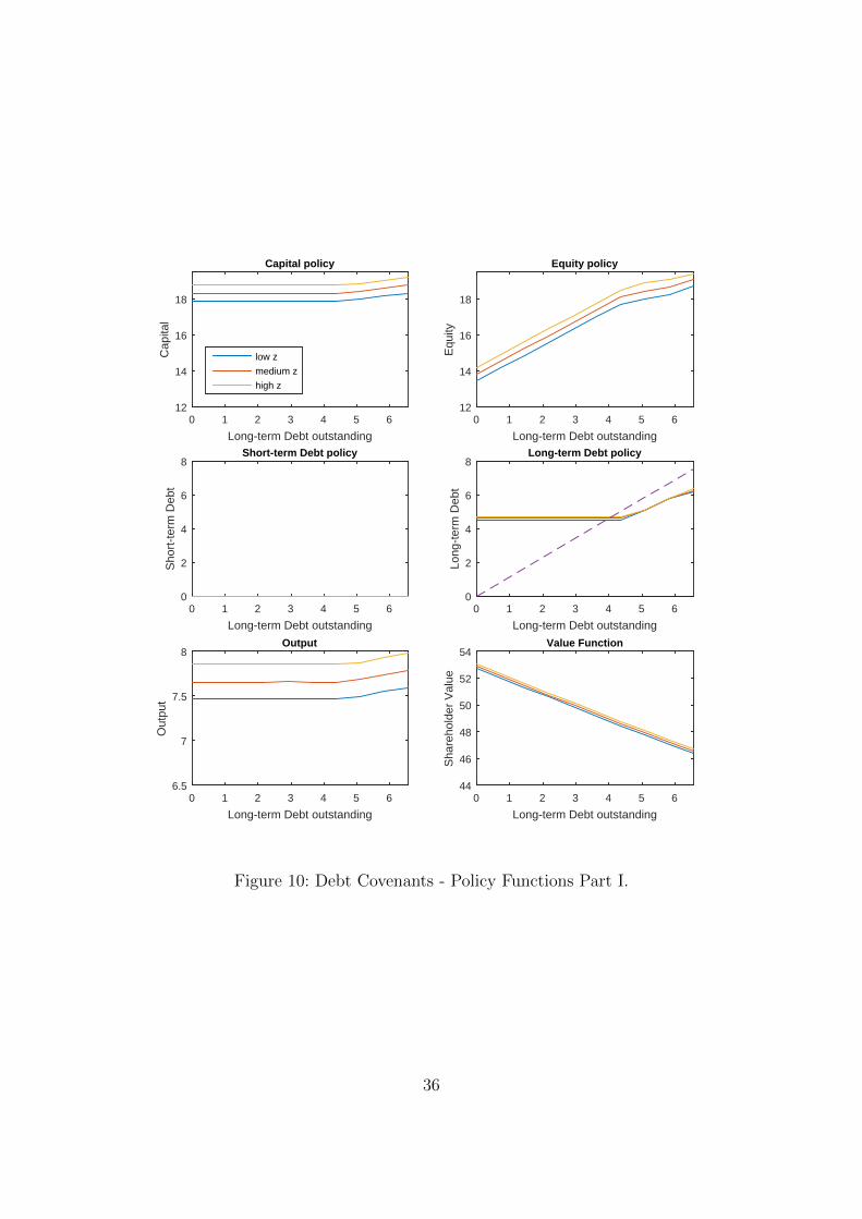
Long-term Debt outstanding0 1 2 3 4 5 6

Cap

ital

12

14

16

18

Capital policy

low z

medium z

high z


Equ

ity

12

14

16

18

Equity policy


Sho

rt-t

erm

Deb

t

0

2

4

6

8Short-term Debt policy


Long

-ter

m D

ebt

0

2

4

6

8Long-term Debt policy


Out

put

6.5

7

7.5

8Output


Sha

reho

lder

Val

ue

44

46

48

50

52

54Value Function

Figure 10: Debt Covenants - Policy Functions Part I.

36


Def

ault

rate

0

0.02

0.04

0.06

0.08

0.1Default rate

low z

medium z

high z


Leve

rage

0

0.2

0.4

0.6

0.8Leverage


Sho

rt-t

erm

Bon

d S

prea

d

0

0.01

0.02

0.03

0.04

0.05Short-term Bond Spread


Long

-ter

m B

ond

Spr

ead

0

0.01

0.02

0.03

0.04

0.05Long-term Bond Spread

Long-term Debt outstanding0 1 2 3 4 5 6T

erm

Str

uctu

re o

f Bon

d S

prea

ds

-0.02

-0.01

0

0.01Term Structure of Bond Spreads


Sha

re o

f Lon

g-te

rm L

iabi

litie

s

0.4

0.6

0.8

1

Share of Long-term Liabilities

Figure 11: Debt Covenants - Policy Functions Part II.

37

As long as b is not ‘too high’, the firm’s choice of k, bS, bL, pS, and ˆpL is independentof b. The reference price pL is falling in b, but overall the reference value of outstandingdebt pLb increases in b. It follows that e′ must rise. As the stock of outstanding debt bincreases, less fresh capital can be raised on the bond market for a given desired level ofleverage. Shareholders have to make up for the difference by injecting additional equityinto the firm.

In the right panel of the middle row of Figure 10, we see that firms always choose tostay within the lower range of b where the default rate, bond spreads, leverage, and theshare of long-term debt are constant in z and b. But why does the firm policy changefor high values of b? The firm maximizes the total return to capital. As b rises, moreof the firm’s earnings are promised to the holders of outstanding long-term bonds andless is available to compensate agents who provide new capital: the shareholders andthe buyers of newly issued debt. This makes the firm less profitable. As b rises beyonda certain point, the marginal unit of capital required to maintain a constant risk ofdefault would earn a negative expected return. This marginal unit of capital is providedby shareholders as b is already above the desired level. At this point, the firm decidesto inject less additional equity than needed to maintain a constant risk of default. Therisk of default, credit spreads, and leverage begin to increase together with b.

As in the first policy experiment, we consider the unexpected introduction of the debtcovenant in period tp = 100. We assume that all outstanding long-term bonds withoutcovenants in tp are swapped with new long-term bonds which feature the covenant.Figure 12 shows what happens in our model economy after the policy intervention attime tp = 100.

Compared to the ban of long-term debt considered in the first policy experiment,the response of the default rate, leverage, and bond spreads is more immediate. In thefirst policy experiment, debt dilution was gradually phased out as long-term debt wasslowly repaid over time. Now we study an immediate and complete neutralization ofdebt dilution. Firms’ equilibrium policy changes on impact. The new default rate isabout 1% compared to almost 3% before the policy intervention. Leverage falls from43% to 25.2%, credit spreads from 1.5% to 0.24%. It follows that debt dilution aloneaccounts for 84% of the credit spread. Although leverage and the default rate are higherthan after the ban of long-term debt studied above, the spread is lower. This is becausethe liquidation value in case of default is higher now (because ε is higher). While theshare of long-term debt jumps up to 1 after the introduction of the debt covenant, theabsolute amount of long-term debt falls.

As in the first policy experiment, output, capital, and welfare all increase in responseto the introduction of the debt covenant. Compared to the ban of long-term debt, lever-age falls by less and credit spreads fall by more. Together, this implies that output,capital, and welfare all increase more strongly compared to the ban of long-term debt.Compensation payments are a more efficient way to tackle firms’ time-inconsistencyproblem as they allow long-term debt to play its socially useful role in reducing transac-tion costs on the bond market. The policy intervention reduces 25% of the total welfaregap with respect to the first best allocation without taxation and with frictionless capitalmarkets.

38

5010

015

020

00

0.51

1.52

Z

5010

015

020

0

-100-9

0

-80

-70

Ou

tpu

t G

ap in

%

5010

015

020

0

-100-9

0

-80

-70

Cap

ital

Gap

in %

5010

015

020

0

-100-9

0

-80

-70

Wel

fare

Gap

in %

5010

015

020

01415161718

Eq

uit

y

5010

015

020

00510

Deb

t

Long

-ter

m D

ebt

Sho

rt-t

erm

Deb

t

5010

015

020

00

0.1

0.2

0.3

0.4

Lev

erag

e

5010

015

020

00

0.51

Lo

ng

-ter

m D

ebt

Sh

are

5010

015

020

00123

Def

ault

Rat

e in

%

5010

015

020

00

0.00

5

0.01

0.01

5

0.02

Sh

ort

-ter

m S

pre

ad

5010

015

020

00

0.00

5

0.01

0.01

5

0.02

Lo

ng

-ter

m S

pre

ad

5010

015

020

01.

081.1

1.12

1.14

Ret

urn

on

Eq

uit

y

Figure 12: Compensation Payments.

39

The last panel of Figure 12 shows the return on equity: 1e′

∫∞εq′ϕ(ε)dε. The return

on equity falls on impact in tp = 100. The sudden and unexpected introduction ofthe debt covenant imposes compensation payments on shareholders. For the holders ofoutstanding long-term debt this is a pure windfall profit as they charged a high creditspread when they bought long-term bonds in the past. The return on equity recoversquickly but never returns to its initial level before the policy intervention. The reasonis that the total amount of equity e′ increases substantially. Total dividend paymentsincrease in response to the policy intervention.

A large part of the welfare gap with respect to the first best allocation is due to thecorporate tax τ . Our parametrization uses as baseline value τ = 29.6%. In order tomeasure the cost of debt dilution, we calculate the reduction in τ which is just enough togenerate the same welfare gain in our benchmark economy as the complete elimination ofdebt dilution. We find that the welfare gain from eliminating debt dilution correspondsto a tax cut of 2.5 percentage points.

Debt Covenants in Practice

We have seen that debt covenants can be a powerful instrument to contain debt dilution.They benefit both shareholders and the economy as a whole. While many different kindsof debt covenants are commonly included in publicly traded bonds, compensation pay-ments like the ones considered in the policy experiment above are not used in practice.21

Debt covenants often prohibit the firm from issuing additional debt of higher seniority.However, covenants which restrict firms to issue additional debt of identical seniority(e.g. through leverage limits or minimum interest coverage ratios) are far less common.

Nash, Netter, and Poulsen (2003) find that 15.66% of 364 investment grade bondissues in 1989 and in 1996 feature restrictions on additional debt of identical seniority.22

In a sample of 100 bond issues 1999-2000, Begley and Freedman (2004) report that 9%contain additional borrowing restrictions.23 Billett et al. (2007) calculate that 17.5%of 15,504 investment grade bond issued between 1960 and 2003 had a covenant whichrestricted future borrowing of identical seniority.24 Reisel (2014) finds in a sample of4,267 bond issues from 1989 - 2006 that 5.9% of investment grade bonds feature covenantswhich restrict additional borrowing.25

In summary, the empirical literature on debt covenants finds that less than twentypercent of investment grade bonds issued by U.S. companies include covenants whichrestrict borrowing of identical seniority.

21Typical debt covenants are cross-default provisions which trigger default as soon as a firm defaultson another liability. Also, covenants commonly restrict the sale of certain firm assets or specify thestatus of debt in case of a merger. For an overview of the usage of different kinds of debt covenants,see for instance the descriptive statistics in Table III of Billett, King, and Mauer (2007).

22Of the 496 bonds considered in their Compustat sample, 120 feature additional debt restrictions(Table 3, p. 218). Of those, 57 bonds are investment grade (Table 4, p.220). It follows that out of atotal of 364 investment grade bonds (Table 2, p.216), 15.66% (or 57) feature additional debt restrictions.

23See their Table 2, p. 24.24See their Table III, p. 707.25See her Table 4, p. 259.

40

6. Conclusion

This paper introduces a maturity choice to the standard model of firm financing andinvestment. We find that debt dilution plays an important role in the trade-off betweenshort-term debt and long-term debt. The intensity of debt dilution varies over thebusiness cycle. During recessions, firms disregards a larger fraction of the total potentialcosts of default. This mechanism generates the observed counter-cyclical behavior ofdefault, bond spreads, leverage, and debt maturity. It also generates the pro-cyclicalterm structure of corporate bond spreads.

Debt dilution renders the equilibrium outcome constrained-inefficient. Credit spreadsare too high and investment is too low. Given that long-term debt induces high defaultrates, firms would like to commit to a policy which uses a smaller amount of long-termdebt in the future. But firms’ time-inconsistency problem also affects their maturitychoice. As the stock of outstanding long-term debt increases, firms internalize a smallerfraction of the entire value of debt. They disregard a larger fraction of the total futurecost of debt dilution and choose a higher share of long-term debt. We show in our firstpolicy experiment that a ban of long-term debt improves welfare in our model economyby reducing credit spreads and increasing investment.

In a second policy experiment, we compare the equilibrium of our benchmark economyto an alternative economy in which long-term bond contracts feature a debt covenantwhich eliminates debt dilution. We find that debt dilution alone accounts for 84% ofthe credit spread and 25% of the welfare gap with respect to the first best allocation.The welfare gain from eliminating debt dilution corresponds to a cut in the corporateincome tax of 2.5 percentage points.

A number of unanswered questions remain. Most importantly, several key results ofthis paper could change once one considers a model economy with more heterogeneityin the firm distribution. In our model, most firms choose identical policies. In thedata, leverage and the distance to default vary considerably across firms. Cooley andQuadrini (2001), Hennessy and Whited (2005), and Covas and Den Haan (2012) showhow to replicate a number of these cross-sectional patterns using models with costlyequity issuance.

Given our parametrization, cyclical debt dilution generates only a modest amount ofamplification. We know that the amount of amplification in our model increases in theequilibrium probability of default. Since most firms in our model economy are identicaland since the average rate of default in the data is low, it is not surprising that ourmodel generates little amplification. This result could change in a model where firmsare more different from the ‘average firm’. In particular, cyclical debt dilution is likelyto strongly affect firms with high leverage and low distance to default.

Also, firms’ maturity choice might become richer in such a model. Long-term debtis a close substitute for equity in the sense that it generates a large inflow of cashtoday in return of small repayments which are extended over several time periods in thefuture. With costly equity issuance, long-term debt becomes more attractive becauseit is a better substitute for equity issuance than short-term debt. An outright ban oflong-term debt might be more costly in a model with costly equity issuance.

41

In our model, a firm’s leverage ratio only changes because of debt dilution. Theremight be additional reasons why a firm chooses to adjust leverage. A model economywhich takes these additional reasons into account could also provide the appropriatelaboratory to study the optimal design of debt covenants. Leverage limits or interestcoverage ratios are beneficial to the extent that they reduce debt dilution. But theymight generate costs as well if they constrain firms in selecting a time-varying level ofleverage.

42

A. Proofs and Derivations

Proof of Proposition 4.1

We divide the first order condition associated to ε by k:

[1− Φ(ε)](1− τ)τc

1 + (1− τ)c− ϕ(ε)(1 + c)

1 + (1− τ)[z f(k)

k− δ + ε

]1 + (1− τ)c

− b

k

= 0 .

In case b = 0, this is equivalent to:

[1− Φ(ε)](1− τ)τc− ϕ(ε)(1 + c) (1 + (1− τ) [−δ + ε]) = ϕ(ε)(1 + c)(1− τ)zf(k)

k.

The first order condition associated to k can be re-arranged as:

− 1 +1 + c

1 + r[1− Φ(ε)]

1 + (1− τ)[−δ + ε]

1 + (1− τ)c+

1− τ1 + r

∫ ∞ε

[ε− ε] ϕ(ε) dε

= − 1 + c

1 + r[1− Φ(ε)]

(1− τ)

1 + (1− τ)czf ′(k) .

Using the property of f(k) that the marginal product is a constant fraction of its averageproduct, we can combine these two first order conditions. We are left with a singleequation with ε as the only endogenous variable. Neither aggregate productivity z nork appear in this equation. It follows that the optimal choice of ε and the the defaultrate Φ(ε) do not depend on z if b = 0. This implies that the bond price p and the creditspread rb − r are constant as well.

What about leverage?

b

k=

1 + (1− τ)[z f(k)

k− δ + ε

]1 + (1− τ)c

.

We know from the first order condition associated to ε that z f(k)k

must be constant in z

if ε does not move and b = 0. It follows that leverage bk

is constant in z if b = 0.Now we consider the case b > 0. The first order condition of k remains unchanged.

With b > 0, there is an additional term added to the marginal benefit of ε. This termis equal to:

b

kϕ(ε) (1 + c) .

This term is positive and increasing in b. By adding this term to the firm’s first ordercondition, the solution for ε is increased. The optimal choice of ε is raised by less if k ishigher. Since the optimal choice of k is increasing in z, it follows that a high value of zimplies a low value of ε if b > 0. It follows that ε and the default rate Φ(ε) are fallingin z if b > 0. This implies that the bond price p rises and the credit spread rb − r falls

43

in z.

Proof of Proposition 4.2

We see immediately that b does not show up in the firm’s problem. The first ordercondition for k is the same as in the case without compensation payments. The firstorder condition for ε is:

ε : [1− Φ(ε)]

[(1 + c)

∂b

∂ε− (1− τ)k

]− ϕ(ε)(1 + c)b = 0 .

It follows that a firm which needs to compensate creditors for changes in the value ofpreviously issued bonds will take exactly the same decisions as a firm which does nothave any long-term debt outstanding (b = 0).

B. Additional Quantitative Results

B.1. The Firm’s Objective Function

Figure 13 shows the firm objective as a function of the firm’s three choice variables:capital k, the threshold value ε, and the long-term debt share m. The firm’s state(b, z) = (2.51, 1), tomorrow’s price of long-term debt pL(s′, φ(s′)), and tomorrow’s firmpolicy φ(s′) are taken as given. The firm’s objective around the global optimum isstrictly concave in all three choice variables. The three panels show the firm’s objectiveas a function of k and ε (top), of k and m (middle), and of ε and m (bottom). In all threepanels, the omitted third choice variable (m, ε, and k, respectively) is held constant atits optimal value. The pink dot indicates the firm’s choice.

B.2. A model without Long-term Debt

In Figure 14, we show the equilibrium policy functions of a model in which firms arenot allowed to issue long-term debt. In the absence of long-term debt, the amount ofdebt issued in the previous period is irrelevant for the firm’s optimal policy. Equity,debt, and capital are pro-cyclical just as in our benchmark model with long-term debt.Leverage, the default rate, and the bond spread are a-cyclical. The firms’ choices arehighly similar to the equilibrium policies from our benchmark economy for b = 0. Figure15 shows impulse response functions after a negative drop in z.

44

48.4

48.6

22

48.8

49

20

49.2

49.4

Given m, B = 2.1899: K = 17.9443, ε = -1.1789, m = 0.64263.

-0.618 -0.8

Capital

16 -1

Epsbar

-1.214 -1.412 -1.6

ValueOptimum

49.1522

49.2

20 0.660.65518

49.25

Given ε, B = 2.1899: K = 17.9443, ε = -1.1789, m = 0.64263.

Capital

0.6516

Maturity

0.645

49.3

14 0.640.63512 0.63

ValueOptimum

48.8-0.6

49

-0.8 0.660.655-1

49.2

Given K, B = 2.1899: K = 17.9443, ε = -1.1789, m = 0.64263.

Epsbar

0.65

Maturity

-1.2 0.645

49.4

0.64-1.4 0.635-1.6 0.63

ValueOptimum

Figure 13: Firm Objective.

45

Debt yesterday0 2 4 6

Cap

ital

12

14

16

18

20Capital policy

low z

medium z

high z


Equ

ity

12

14

16

18

20Equity policy


Deb

t

0

2

4

6

8

10Debt policy


Leve

rage

0

0.1

0.2

0.3

0.4

0.5Leverage


Def

ault

rate

0

0.01

0.02

0.03Default rate


Bon

d S

prea

d

0

0.005

0.01

0.015Bond Spread

Figure 14: A model without Long-term Debt - Policy Functions

46

1020

3040

500.

992

0.99

4

0.99

6

0.99

81Z

1020

3040

500.

97

0.98

0.991

Ou

tpu

t

1020

3040

500.

97

0.98

0.991

Cap

ital

1020

3040

500.

97

0.98

0.991

Eq

uit

y

1020

3040

500.

97

0.98

0.991

Deb

t

1020

3040

500

0.51

Lev

erag

e

1020

3040

50

0.5

0.6

0.7

Def

ault

Rat

e in

%

1020

3040

500

0.00

5

0.01

Bo

nd

Sp

read

Figure 15: A model without Long-term Debt - Impulse Response Functions

47

References

Adrian, T., P. Colla, and H. S. Shin (2012): “Which financial frictions? Parsingthe evidence from the financial crisis of 2007 to 2009,” in NBER MacroeconomicsAnnual 2012, Volume 27, University of Chicago Press, 159–214.

Aguiar, M., M. Amador, H. Hopenhayn, and I. Werning (2016): “Take theShort Route: Equilibrium Default and Debt Maturity,” Working Paper 22847, Na-tional Bureau of Economic Research.

Altınkılıc, O. and R. S. Hansen (2000): “Are there economies of scale in under-writing fees? Evidence of rising external financing costs,” Review of financial Studies,13, 191–218.

Arellano, C. and A. Ramanarayanan (2012): “Default and the Maturity Struc-ture in Sovereign Bonds,” Journal of Political Economy, 120, 187 – 232.

Begley, J. and R. Freedman (2004): “The changing role of accounting numbers inpublic lending agreements,” Accounting Horizons, 18, 81–96.

Billett, M. T., T.-H. D. King, and D. C. Mauer (2007): “Growth opportunitiesand the choice of leverage, debt maturity, and covenants,” The Journal of Finance,62, 697–730.

Bris, A., I. Welch, and N. Zhu (2006): “The costs of bankruptcy: Chapter 7liquidation versus Chapter 11 reorganization,” The Journal of Finance, 61, 1253–1303.

Caggese, A. and A. Perez (2015): “The Interaction between Household and FirmDynamics and the Amplification of Financial Shocks,” Working Paper 866, BarcelonaGSE.

Calvo, G. A. (1988): “Servicing the Public Debt: The Role of Expectations,” Ameri-can Economic Review, 78, 647–61.

Carlstrom, C. T. and T. S. Fuerst (1997): “Agency costs, net worth, and busi-ness fluctuations: A computable general equilibrium analysis,” American EconomicReview, 87, 893–910.

Chatterjee, S. and B. Eyigungor (2012): “Maturity, Indebtedness, and DefaultRisk,” American Economic Review, 102, 2674–2699.

——— (2015): “A seniority arrangement for sovereign debt,” American Economic Re-view, 105, 3740–3765.

Cooley, T. F. and V. Quadrini (2001): “Financial Markets and Firm Dynamics,”American Economic Review, 91, 1286–1310.

48

Covas, F. and W. J. Den Haan (2012): “The Role of Debt and Equity FinanceOver the Business Cycle,” The Economic Journal, 122, 1262–1286.

Crouzet, N. (2016): “Default, debt maturity, and investment dynamics,” WorkingPaper.

Elton, E. J., M. J. Gruber, D. Agrawal, and C. Mann (2001): “Explaining therate spread on corporate bonds,” The Journal of Finance, 56, 247–277.

Giesecke, K., F. A. Longstaff, S. Schaefer, and I. A. Strebulaev (2014):“Macroeconomic effects of corporate default crisis: A long-term perspective,” Journalof Financial Economics, 111, 297–310.

Gilchrist, S. and E. Zakrajsek (2012): “Credit Spreads and Business Cycle Fluc-tuations,” American Economic Review, 102, 1692–1720.

Gomes, J., U. Jermann, and L. Schmid (2016): “Sticky Leverage,” AmericanEconomic Review, 106, 3800–3828.

Gomes, J. and L. Schmid (2016): “Equilibrium Asset Pricing with Leverage andDefault,” Working Paper.

Gomes, J., A. Yaron, and L. Zhang (2003): “Asset Prices and Business Cycleswith Costly External Finance,” Review of Economic Dynamics, 6, 767–788.

Gourio, F. and M. Michaux (2012): “Financing Investment with Long-Term Debtand Uncertainty Shocks,” Working Paper.

Hatchondo, J. C. and L. Martinez (2009): “Long-duration bonds and sovereigndefaults,” Journal of International Economics, 79, 117–125.

——— (2013): “Sudden stops, time inconsistency, and the duration of sovereign debt,”International Economic Journal, 27, 217–228.

Hatchondo, J. C., L. Martinez, and C. Sosa-Padilla (2016): “Debt Dilutionand Sovereign Default Risk,” Journal of Political Economy, 124, 1383–1422.

Hennessy, C. A. and T. M. Whited (2005): “Debt dynamics,” The Journal ofFinance, 60, 1129–1165.

Jermann, U. and V. Quadrini (2012): “Macroeconomic Effects of Financial Shocks,”American Economic Review, 102, 238–271.

Leland, H. (1994): “Bond prices, yield spreads, and optimal capital structure withdefault risk,” Working Paper.

Miao, J. and P. Wang (2010): “Credit Risk and Business Cycles,” Working Paper.

49

Nash, R. C., J. M. Netter, and A. B. Poulsen (2003): “Determinants of contrac-tual relations between shareholders and bondholders: investment opportunities andrestrictive covenants,” Journal of Corporate Finance, 9, 201–232.

Nicolini, J. P., P. Teles, J. L. Ayres, and G. Navarro (2015): “SovereignDefault: The Role of Expectations,” Working Paper.

Quadrini, V. (2011): “Financial frictions in macroeconomic fluctuations,” FRB Rich-mond Economic Quarterly, 97, 209–254.

Ravn, M. O. and H. Uhlig (2002): “On adjusting the Hodrick-Prescott filter for thefrequency of observations,” Review of economics and statistics, 84, 371–376.

Reisel, N. (2014): “On the value of restrictive covenants: Empirical investigation ofpublic bond issues,” Journal of Corporate Finance, 27, 251–268.

Sachs, J. and D. Cohen (1982): “LDC Borrowing with Default Risk,” in NBERWorking Paper 925.

50

Optimal Debt Maturity and Firm Investment

Documents

Transcript of Optimal Debt Maturity and Firm Investment