Optimal Control of Partial Di erential...
102
Optimal Control of Partial Differential Equations Peter Philip * Lecture Notes Originally Created for the Class of Spring Semester 2007 at HU Berlin, Revised and Extended for the Class of Spring Semester 2009 at LMU Munich † October 17, 2013 Contents 1 Motivating Examples 4 1.1 Stationary Optimal Heating Problems ................... 4 1.1.1 General Setting ........................... 4 1.1.2 Boundary Control .......................... 5 1.1.3 Distributed Control ......................... 7 1.2 Transient Optimal Heating Problems ................... 8 1.2.1 General Setting ........................... 8 1.2.2 Boundary Control .......................... 9 1.2.3 Distributed Control ......................... 10 2 Convexity 10 2.1 Basic Definitions and Criteria for Convex Functions ........... 11 2.2 Relation Between Convexity and the Uniqueness of Extrema ...... 17 3 Review: Finite-Dimensional Optimization 18 * E-Mail: [email protected] † Roughly based on Fredi Tr¨ oltzsch [Tr¨ o05]. I wish to thank Olaf Klein for pointing out several errors contained in my original manuscript. Any remaining errors contained in the lecture notes are solely my responsibility. 1
Transcript of Optimal Control of Partial Di erential...
Optimal Control of Partial Differential Equations
Peter Philip∗
Lecture Notes
Originally Created for the Class of Spring Semester 2007 at HU Berlin,
Revised and Extended for the Class of Spring Semester 2009 at LMU Munich†
October 17, 2013
Contents
1 Motivating Examples 4
1.1 Stationary Optimal Heating Problems . . . . . . . . . . . . . . . . . . . 4
1.1.1 General Setting . . . . . . . . . . . . . . . . . . . . . . . . . . . 4
1.1.2 Boundary Control . . . . . . . . . . . . . . . . . . . . . . . . . . 5
1.1.3 Distributed Control . . . . . . . . . . . . . . . . . . . . . . . . . 7
1.2 Transient Optimal Heating Problems . . . . . . . . . . . . . . . . . . . 8
1.2.1 General Setting . . . . . . . . . . . . . . . . . . . . . . . . . . . 8
1.2.2 Boundary Control . . . . . . . . . . . . . . . . . . . . . . . . . . 9
1.2.3 Distributed Control . . . . . . . . . . . . . . . . . . . . . . . . . 10
2 Convexity 10
2.1 Basic Definitions and Criteria for Convex Functions . . . . . . . . . . . 11
2.2 Relation Between Convexity and the Uniqueness of Extrema . . . . . . 17
3 Review: Finite-Dimensional Optimization 18
∗E-Mail: [email protected]†Roughly based on Fredi Troltzsch [Tro05]. I wish to thank Olaf Klein for pointing out several
errors contained in my original manuscript. Any remaining errors contained in the lecture notes aresolely my responsibility.
1
CONTENTS 2
3.1 A Finite-Dimensional Optimal Control Problem . . . . . . . . . . . . . 18
3.2 Existence and Uniqueness . . . . . . . . . . . . . . . . . . . . . . . . . 20
3.3 First Order Necessary Optimality Conditions, Variational Inequality . . 21
3.4 Adjoint Equation, Adjoint State . . . . . . . . . . . . . . . . . . . . . . 25
3.5 Lagrange Technique and Karush-Kuhn-Tucker Conditions . . . . . . . . 26
3.5.1 Lagrange Function . . . . . . . . . . . . . . . . . . . . . . . . . 26
3.5.2 Box Constraints and Karush-Kuhn-Tucker Optimality Conditions 27
3.6 A Preview of Optimal Control of PDE . . . . . . . . . . . . . . . . . . 29
4 Review: Functional Analysis Tools 30
4.1 Normed Vector Spaces . . . . . . . . . . . . . . . . . . . . . . . . . . . 30
4.2 Bilinear Forms . . . . . . . . . . . . . . . . . . . . . . . . . . . . . . . 31
4.3 Hilbert Spaces . . . . . . . . . . . . . . . . . . . . . . . . . . . . . . . . 32
4.4 Bounded Linear Operators . . . . . . . . . . . . . . . . . . . . . . . . . 34
4.5 Adjoint Operators . . . . . . . . . . . . . . . . . . . . . . . . . . . . . . 36
4.6 Weak Convergence . . . . . . . . . . . . . . . . . . . . . . . . . . . . . 38
5 Optimal Control in Reflexive Banach Spaces 42
5.1 Existence and Uniqueness . . . . . . . . . . . . . . . . . . . . . . . . . 42
5.2 Applications . . . . . . . . . . . . . . . . . . . . . . . . . . . . . . . . . 44
5.2.1 Existence of an Orthogonal Projection . . . . . . . . . . . . . . 44
5.2.2 Lax-Milgram Theorem . . . . . . . . . . . . . . . . . . . . . . . 46
6 Optimal Control of Linear Elliptic PDE 49
6.1 Sobolev Spaces . . . . . . . . . . . . . . . . . . . . . . . . . . . . . . . 49
6.1.1 Lp-Spaces . . . . . . . . . . . . . . . . . . . . . . . . . . . . . . 49
6.1.2 Weak Derivatives . . . . . . . . . . . . . . . . . . . . . . . . . . 50
6.1.3 Boundary Issues . . . . . . . . . . . . . . . . . . . . . . . . . . . 53
6.2 Linear Elliptic PDE . . . . . . . . . . . . . . . . . . . . . . . . . . . . . 58
6.2.1 Setting and Basic Definitions, Strong and Weak Formulation . . 58
6.2.2 Existence and Uniqueness of Weak Solutions . . . . . . . . . . . 60
6.3 Optimal Control Existence and Uniqueness . . . . . . . . . . . . . . . . 64
6.4 First Order Necessary Optimality Conditions, Variational Inequality . . 67
6.4.1 Differentiability in Normed Vector Spaces . . . . . . . . . . . . 67
CONTENTS 3
6.4.2 Variational Inequality, Adjoint State . . . . . . . . . . . . . . . 79
6.4.3 Adjoint Equation . . . . . . . . . . . . . . . . . . . . . . . . . . 81
6.4.4 Pointwise Formulations of the Variational Inequality . . . . . . . 83
6.4.5 Lagrange Multipliers and Karush-Kuhn-Tucker Optimality Con-ditions . . . . . . . . . . . . . . . . . . . . . . . . . . . . . . . . 88
7 Introduction to Numerical Methods 90
7.1 Conditional Gradient Method . . . . . . . . . . . . . . . . . . . . . . . 91
7.1.1 Abstract Case: Hilbert Space . . . . . . . . . . . . . . . . . . . 91
7.1.2 Application: Elliptic Optimal Control Problem . . . . . . . . . . 92
7.2 Projected Gradient Method . . . . . . . . . . . . . . . . . . . . . . . . 94
7.3 Transformation into Finite-Dimensional Problems . . . . . . . . . . . . 95
7.3.1 Finite-Dimensional Formulation in Nonreduced Form . . . . . . 95
7.3.2 Finite-Dimensional Formulation in Reduced Form . . . . . . . . 97
7.3.3 Trick to Solve the Reduced Form Without Formulating it First . 98
7.4 Active Set Methods . . . . . . . . . . . . . . . . . . . . . . . . . . . . . 99
1 MOTIVATING EXAMPLES 4
1 Motivating Examples
As motivating examples, we will consider several variants of optimal heating problems.Further examples of applied problems can be found in Sections 1.2 and 1.3 of [Tro05].
1.1 Stationary Optimal Heating Problems
1.1.1 General Setting
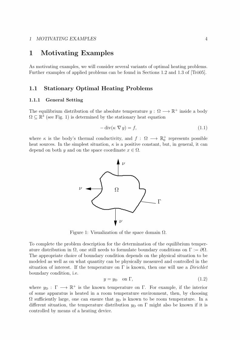
The equilibrium distribution of the absolute temperature y : Ω −→ R+ inside a bodyΩ ⊆ R3 (see Fig. 1) is determined by the stationary heat equation
− div(κ ∇ y) = f, (1.1)
where κ is the body’s thermal conductivity, and f : Ω −→ R+0 represents possible
heat sources. In the simplest situation, κ is a positive constant, but, in general, it candepend on both y and on the space coordinate x ∈ Ω.
Ω
ν
ν
Γ
ν
Figure 1: Visualization of the space domain Ω.
To complete the problem description for the determination of the equilibrium temper-ature distribution in Ω, one still needs to formulate boundary conditions on Γ := ∂Ω.The appropriate choice of boundary condition depends on the physical situation to bemodeled as well as on what quantity can be physically measured and controlled in thesituation of interest. If the temperature on Γ is known, then one will use a Dirichletboundary condition, i.e.
y = yD on Γ, (1.2)
where yD : Γ −→ R+ is the known temperature on Γ. For example, if the interiorof some apparatus is heated in a room temperature environment, then, by choosingΩ sufficiently large, one can ensure that yD is known to be room temperature. In adifferent situation, the temperature distribution yD on Γ might also be known if it iscontrolled by means of a heating device.
1 MOTIVATING EXAMPLES 5
We are now in a position to formulate some first optimal control problems. The generalidea is to vary (i.e. control) an input quantity (called the control, typically denotedby u) such that some output quantity (called the state, typically denoted by y) has adesired property. This desired property is measured according to some function J , calledthe objective function or the objective functional (if it is defined on a space of infinitedimension, as is the case when controlling partial differential equations). Usually, theobjective functional is formulated such that the desired optimal case coincides with aminimum of J . In general, J can depend on both the control u and on the state y.However, if there exists a unique state for each control (i.e. if there is a map S : u 7→y = S(u)), then J can be considered as a function of the control alone. We will mostlyconcentrate on this latter situation, considering partial differential equations that admita unique solution y for each control u.
When controlling partial differential equations (PDE), the state y is the quantity de-termined as the solution of the PDE, whereas the control can be an input functionprescribed on the boundary Γ (so-called boundary control) or an input function pre-scribed on the volume domain Ω (so-called distributed control).
In the context of optimal heating, where the state y is the absolute temperature de-termined as a solution of the heat equation (1.1), we will now consider one example ofboundary control (Sec. 1.1.2) and one example of distributed control (Sec. 1.1.3).
1.1.2 Boundary Control
Consider the case that, for a desired application, the optimal temperature distributionyΩ : Ω −→ R+ is known and that heating elements can control the temperature u := yDat each point of the boundary Γ. The goal is to find u such that the actual temperaturey approximates yΩ. This problem leads to the minimization of the objective functional
J(y, u) :=1
2
∫Ω
(y(x)− yΩ(x)
)2dx +
λ
2
∫Γ
u(x)2 ds(x) , (1.3)
where λ > 0, and s is used to denote the surface measure on Γ. The second integralin (1.3) is a typical companion of the first in this type of problem. It can be seen as ameasure for the expenditure of the control. For instance, in the present example, it canbe interpreted as measuring the energy costs of the heating device. In mathematicalterms, the second integral in (1.3) has a regularizing effect; it is sometimes called aTychonoff regularization. It counteracts the tendency of the control to become locallyunbounded and rugged as J approaches its infimum.
Due to physical and technical limitations of the heating device, one needs to imposesome restrictions on the control u. Physical limitations result from the fact that anydevice will be destroyed if its temperature becomes to high or to low. However, thetechnical limitations of the heating device will usually be much more restrictive, provid-ing upper and lower bounds for the temperatures that the device can impose. Hence,one is led to the control constraints
a ≤ u ≤ b on Γ, (1.4)

1 MOTIVATING EXAMPLES 6
where 0 < a < b. Control constraints of this form are called box constraints.
If, apart from the control, the system does not contain any heat sources, then f ≡ 0 in(1.1) and the entire optimal control problem can be summarized as follows:
Minimize J(y, u) =1
2
∫Ω
(y(x)− yΩ(x)
)2dx +
λ
2
∫Γ
u(x)2 ds(x) , (1.5a)
subject to the PDE constraints
− div(κ ∇ y) = 0 in Ω, (1.5b)
y = u on Γ, (1.5c)
and control constraintsa ≤ u ≤ b on Γ. (1.5d)
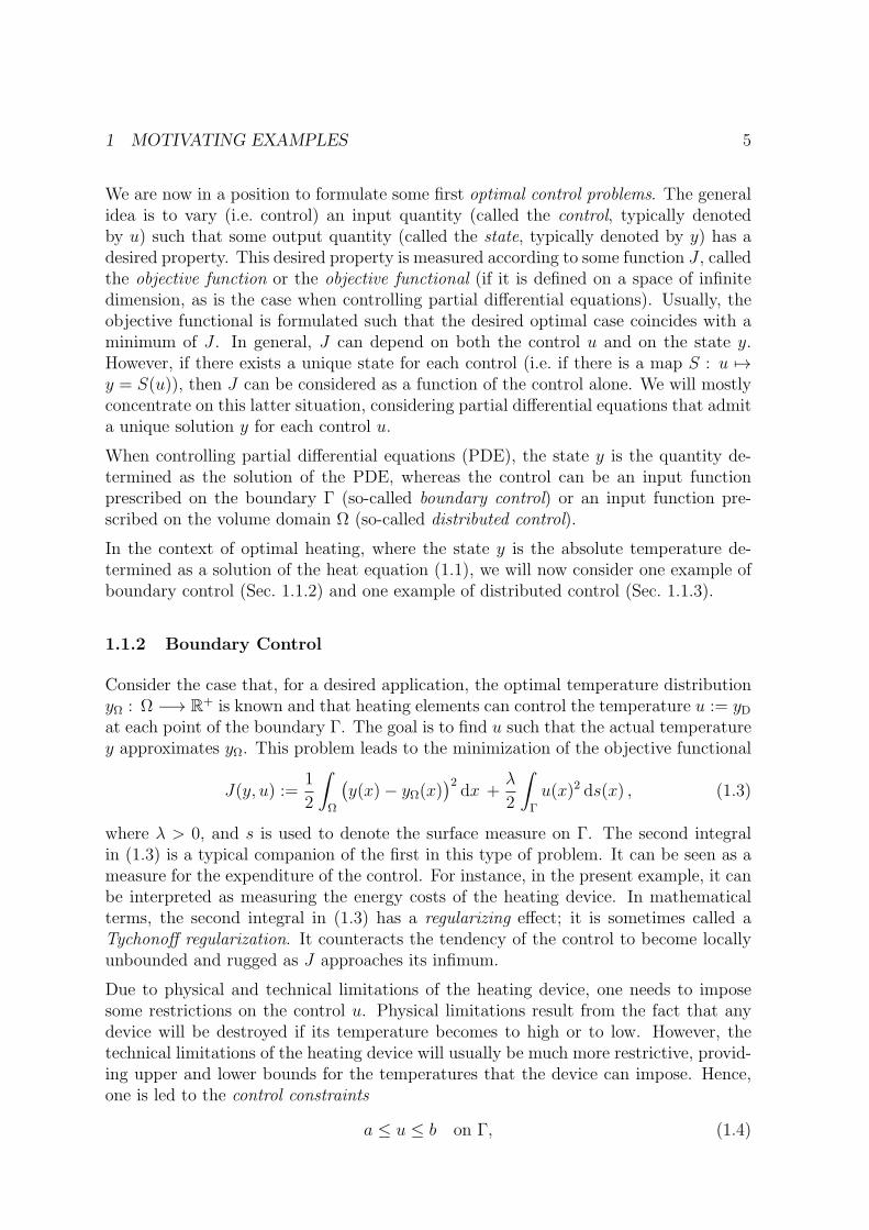
In a slightly more realistic setting, one might only be able to control the temperature onsome part Γc of Γ with Γc ( Γ. For example, the goal might be to homogeneously heata room to a temperature θopt, where the heating element has already been installedat a fixed location with boundary Γc. In this case, (1.5a) needs to be replaced bya version where the second integral is only carried out over Γc. The result is (1.7a)below, where yΩ ≡ θopt was used as well. Since the control is now only given on Γc,(1.5c) and (1.5d) also need to be modified accordingly, leading to (1.7c) and (1.7e),respectively. In consequence, one still needs to specify a boundary condition on Γ \ Γc.If the surrounding environment is at temperature yext, then, according to the Stefan-Boltzmann law of (emitted heat) radiation, the boundary condition reads
∇ y · ν = α (y4ext − y4) on Γ \ Γc, (1.6)
where ν denotes the outer unit normal on Γ, and α is a positive constant.
Summarizing this modified optimal control problem yields the following system (1.7):
Minimize J(y, u) =1
2
∫Ω
(y(x)− θopt
)2dx +
λ
2
∫Γc
u(x)2 ds(x) , (1.7a)
subject to the PDE constraints
− div(κ ∇ y) = 0 in Ω, (1.7b)
y = u on Γc, (1.7c)
∇ y · ν = α (y4ext − y4) on Γ \ Γc, (1.7d)
and control constraintsa ≤ u ≤ b on Γc. (1.7e)
1 MOTIVATING EXAMPLES 7
Ω
ν
ν
Γ \ Γc
A ⊂ R3 \ Ω
Γc
ν
Figure 2: Visualization of the space domain Ω for the optimal heating problem (1.7).
1.1.3 Distributed Control
We now consider the case that we can control the heat sources f inside the domainΩ, setting f = u in (1.1). The control is no longer concentrated on the boundaryΓ, but distributed over Ω. Such distributed heat sources occur, for example, duringelectromagnetic or microwave heating.
As u now lives on Ω, the corresponding integration in the objective functional (cf. (1.5a)and (1.7a)) has to be performed over Ω. Similarly, the control constraints now have tobe imposed on Ω rather than on the boundary. Thus, keeping the Dirichlet conditionfrom (1.2), the complete optimal control problem reads as follows:
Minimize J(y, u) =1
2
∫Ω
(y(x)− yΩ(x)
)2dx +
λ
2
∫Ω
u(x)2 dx , (1.8a)
subject to the PDE constraints
− div(κ ∇ y) = u in Ω, (1.8b)
y = yD on Γ, (1.8c)
and control constraintsa ≤ u ≤ b on Ω. (1.8d)
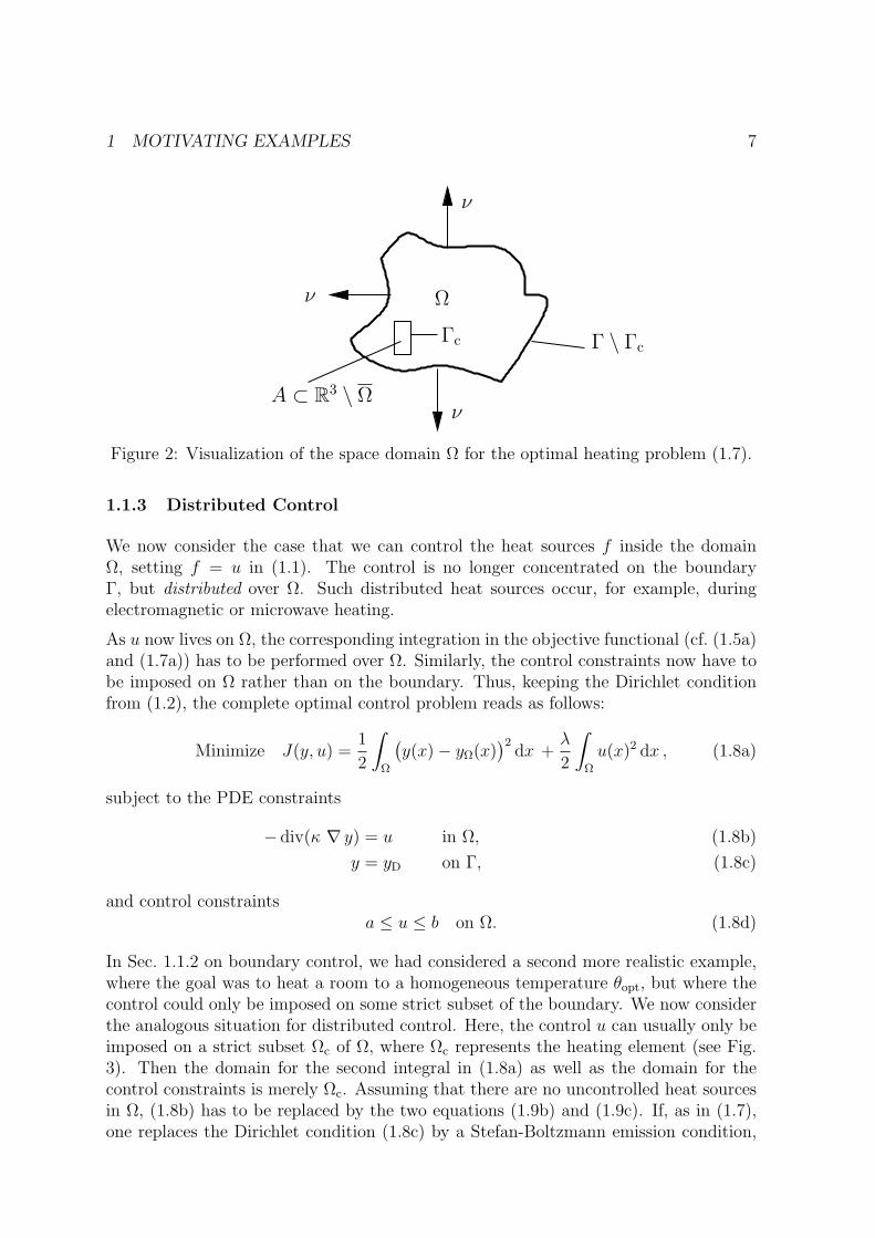
In Sec. 1.1.2 on boundary control, we had considered a second more realistic example,where the goal was to heat a room to a homogeneous temperature θopt, but where thecontrol could only be imposed on some strict subset of the boundary. We now considerthe analogous situation for distributed control. Here, the control u can usually only beimposed on a strict subset Ωc of Ω, where Ωc represents the heating element (see Fig.3). Then the domain for the second integral in (1.8a) as well as the domain for thecontrol constraints is merely Ωc. Assuming that there are no uncontrolled heat sourcesin Ω, (1.8b) has to be replaced by the two equations (1.9b) and (1.9c). If, as in (1.7),one replaces the Dirichlet condition (1.8c) by a Stefan-Boltzmann emission condition,
1 MOTIVATING EXAMPLES 8
then one obtains the following modified version of the optimal control problem (1.8):
Minimize J(y, u) =1
2
∫Ω
(y(x)− θopt
)2dx +
λ
2
∫Ωc
u(x)2 dx , (1.9a)
subject to the PDE constraints
− div(κ ∇ y) = u in Ωc, (1.9b)
− div(κ ∇ y) = 0 in Ω \ Ωc, (1.9c)
∇ y · ν = α (y4ext − y4) on Γ, (1.9d)
and control constraintsa ≤ u ≤ b on Ωc. (1.9e)
Ω
ν
ν
Γ
Ωc ⊆ Ω
ν
Figure 3: Visualization of the space domain Ω for the distributed control problem (1.9).
1.2 Transient Optimal Heating Problems
1.2.1 General Setting
While (1.1) describes the equilibrium temperature distribution inside a body, if thetemperature is (still) changing with time t, then it is governed by the transient heatequation
∂t y − div (κ∇ y) = f, (1.10)
that merely differs from (1.1) by the presence of the partial derivative with respect totime. Of course, in general, the temperature y and the heat sources f can now dependon time as well as on the space coordinate, i.e. they are defined on the so-called time-space cylinder [0, T ]×Ω, where T > 0 represents a final time. Here and in the following,we use 0 as the initial time, which is a customary convention. In the transient situation,one needs another condition for a complete problem formulation. One usually starts
1 MOTIVATING EXAMPLES 9
the evolution from a known temperature distribution at the initial time t = 0, i.e. onestarts with an initial condition
y(0, ·) = y0 in Ω, (1.11)
where y0 : Ω −→ R+ is the known initial temperature in Ω.
Each of the optimal control examples considered in Sec. 1.1 can also be consideredin a corresponding time-dependent setting. Instead of trying to generate a desiredequilibrium temperature yΩ, one might want to reach yΩ already for t = T . At thesame time, it might be possible to vary the control u with time. As in Sec. 1.1, weconsider the case, where u controls the temperature on (some part of) the boundary(boundary control, see Sec. 1.2.2), and the case, where u controls the heat sources inside(some part of) Ω (see Sec. 1.2.3).
1.2.2 Boundary Control
The objective functional J (cf. 1.5a) needs to be modified to be suitable for the time-dependent situation. As the temperature y now depends on both time and space, andas the desired temperature field yΩ should be approximated as good as possible at thefinal time T , y(T, ·) occurs in the first integral in J . The second integral, involving thecontrol u, now needs to be carried out over the time domain as well as over the spacedomain (see (1.12a)). In the PDE and control constraints, the only modifications arethat the constraints are now considered in the respective time-space cylinders and thatthe initial condition (1.11) is added. Thus, the transient version of (1.5) reads:
Minimize J(y, u) =1
2
∫Ω
(y(T, x)− yΩ(x)
)2dx +
λ
2
∫ T
0
∫Γ
u(t, x)2 ds(x) dt , (1.12a)
subject to the PDE constraints
∂t y − div (κ∇ y) = 0 in [0, T ]× Ω, (1.12b)
y = u on [0, T ]× Γ, (1.12c)
y(0, ·) = y0 in Ω, (1.12d)
and control constraintsa ≤ u ≤ b on [0, T ]× Γ. (1.12e)
Similarly, one obtains the following transient version of (1.7):
Minimize J(y, u) =1
2
∫Ω
(y(T, x)− θopt
)2dx +
λ
2
∫ T
0
∫Γc
u(t, x)2 ds(x) dt , (1.13a)
subject to the PDE constraints
∂t y − div (κ∇ y) = 0 in [0, T ]× Ω, (1.13b)
y = u on [0, T ]× Γc, (1.13c)
∇ y · ν = α (y4ext − y4) on [0, T ]× (Γ \ Γc), (1.13d)
y(0, ·) = y0 in Ω, (1.13e)
2 CONVEXITY 10
and control constraintsa ≤ u ≤ b on [0, T ]× Γc. (1.13f)
1.2.3 Distributed Control
The way one passes from the stationary to the corresponding transient control problemsis completely analogous to the boundary control problems. The first integral in theobjective functional J now involves the temperature at the final time T while thesecond integral is over both space and time. Furthermore, space domains are replacedby time-space cylinders and the initial condition (1.11) is added. Thus, one obtains thetransient version of (1.8):
Minimize J(y, u) =1
2
∫Ω
(y(T, x)− yΩ(x)
)2dx +
λ
2
∫ T
0
∫Ω
u(t, x)2 dx dt , (1.14a)
subject to the PDE constraints
∂t y − div (κ∇ y) = u in [0, T ]× Ω, (1.14b)
y = yD on [0, T ]× Γ, (1.14c)
y(0, ·) = y0 in Ω, (1.14d)
and control constraintsa ≤ u ≤ b on [0, T ]× Ω. (1.14e)
Analogously, one obtains the transient version of (1.9):
Minimize J(y, u) =1
2
∫Ω
(y(T, x)− θopt
)2dx +
λ
2
∫ T
0
∫Ωc
u(t, x)2 dx dt , (1.15a)
subject to the PDE constraints
∂t y − div(κ ∇ y) = u in [0, T ]× Ωc, (1.15b)
∂t y − div(κ ∇ y) = 0 in [0, T ]× Ω \ Ωc, (1.15c)
∇ y · ν = α (y4ext − y4)on [0, T ]× Γ, (1.15d)
y(0, ·) = y0 in Ω, (1.15e)
and control constraintsa ≤ u ≤ b on [0, T ]× Ωc. (1.15f)
2 Convexity
It is already well-known from finite-dimensional optimization that a unique minimumof the objective function can, in general, not be expected if the objective function isnot convex. On the other hand, as we will see in Th. 2.17, strict convexity of the
2 CONVEXITY 11
objective function does guarantee uniqueness. Therefore, according to the properties ofthe considered objective functional, optimal control problems are often classified intoconvex and nonconvex problems.
We start by reviewing the basic definitions of convex sets and functions in Sec. 2.1,where we will also study sufficient conditions for functions to be convex. These willlater be useful to determine the convexity properties of objective functionals.
In Sec. 2.2, we provide the relevant results regarding the relation between the uniquenessof extreme values of functions and the functions’ convexity properties.
2.1 Basic Definitions and Criteria for Convex Functions
Definition 2.1. A subset C of a real vector space X is called convex if, and only if,for each (x, y) ∈ C2 and each 0 ≤ α ≤ 1, one has αx+ (1− α) y ∈ C.
Lemma 2.2. Let X, Y be real vector spaces, let C1 ⊆ X, C2 ⊆ Y be convex. ThenC1 × C2 is a convex subset of X × Y .
Proof. Let (x1, x2) ∈ C21 , (y1, y2) ∈ C2
2 , α ∈ [0, 1]. Then
α (x1, y1) + (1− α) (x2, y2) =(αx1 + (1− α) x2, α y1 + (1− α) y2
)∈ C1 × C2 (2.1)
as αx1 + (1−α) x2 ∈ C1 and α y1 + (1−α) y2 ∈ C2 due to the convexity of C1 and C2,respectively.
Definition 2.3. Let C be a convex subset of a real vector space X.
(a) A function J : C −→ R∪+∞ is called convex if, and only if, for each (x, y) ∈ C2
and each 0 ≤ α ≤ 1:
J(αx+ (1− α) y
)≤ αJ(x) + (1− α) J(y). (2.2a)
If the inequality in (2.2a) is strict whenever x 6= y and 0 < α < 1, then J is calledstrictly convex.
(b) A function S : C −→ Y , where Y is another real vector space, is said to preserveconvex combinations if, and only if, (x, y) ∈ C2 and each 0 ≤ α ≤ 1:
S(αx+ (1− α) y
)= αS(x) + (1− α)S(y). (2.2b)
Note that, if S preserves convex combinations, then S(C) is also convex: If a, b ∈S(C), then there are x, y ∈ C such that S(x) = a and S(y) = b, and, if 0 ≤ α ≤ 1and S preserve convex combinations, then
αa+ (1− α)b = αS(x) + (1− α)S(y) = S(αx+ (1− α)y
),
showing αa+ (1− α)b ∈ S(C).
2 CONVEXITY 12
Remark 2.4. Let X,Y be a real vector spaces, let C ⊆ X be convex. Then S : C −→Y preserves convex combinations if, and only if, S is the restriction of an affine mapA : X −→ Y (i.e. if, and only if, there exists a linear map L : X −→ Y and a ∈ X suchthat A = L+ a and S = AC : Suppose S is the restriction of an affine map A = L+ awith L and a as above. Then, for each (x, y) ∈ C2 and each 0 ≤ α ≤ 1,
S(αx+ (1− α) y
)= αLx+ (1− α)Ly + a = α (Lx+ a) + (1− α) (Ly + a)
= αS(x) + (1− α)S(y), (2.3)
showing that S preserves convex combinations. Conversely, assume S preserves convexcombinations. Fix c ∈ C. Then there exists a linear map L : X −→ Y such that L(x) =S(x+ c)− S(c) for each x ∈ X with x+ c ∈ C (as S preserves convex combinations, itcanonically extends to the affine hull aff(C) of C, i.e. L(x) = S(x+ c)− S(c) defines alinear map on the linear subspace V := aff(C) − c of X, which can then be extendedto all of X). Thus, letting a := −L(c) + S(c), we obtain, for each x ∈ C: A(x) =L(x) + a = L(x)− L(c) + S(c) = L(x− c) + S(c) = S(x− c+ c)− S(c) + S(c) = S(x).
If S preserves convex combinations and X = R, then S is convex, but not strictlyconvex if C consists of more than one point.
Lemma 2.5. Let X be a real vector space, let C ⊆ X be convex.
(a) If Y is a real vector space, f : C −→ Y preserves convex combinations and g :f(C) −→ R is convex, then g f is convex. If, moreover, f is one-to-one and g isstrictly convex, then g f is strictly convex.
(b) Suppose f : C −→ R, let I ⊆ R be convex such that f(C) ⊆ I and g : I −→ R. Iff and g are both convex and g is increasing, then g f is convex. If, in addition,at least one of the following conditions (i), (ii) holds, where(i) f is strictly convex and g is strictly increasing,(ii) f is one-to-one and g is strictly convex,then g f is strictly convex.
(c) If λ ∈ R+ and f : C −→ R is (strictly) convex, then λf is (strictly) convex.
Proof. Let (x, y) ∈ C2, α ∈ [0, 1].
(a): The hypotheses on f and g yield
(g f)(αx+ (1− α) y
)= g(f(αx+ (1− α) y
))= g(α f(x) + (1− α) f(y)
)≤ α g
(f(x)
)+ (1− α) g
(f(y)
)= α (g f)(x) + (1− α) (g f)(y), (2.4)
showing that g f is convex. If f is one-to-one and g is strictly convex, then theinequality in (2.4) is strict for x 6= y and 0 < α < 1, showing that g f is strictlyconvex.
2 CONVEXITY 13
(b): The convexity of f yields
f(αx+ (1− α) y
)≤ α f(x) + (1− α) f(y). (2.5)
As g is increasing, one obtains from (2.5)
(g f)(αx+ (1− α) y
)= g(f(αx+ (1− α) y
))≤ g(α f(x) + (1− α) f(y)
)≤ α g
(f(x)
)+ (1− α) g
(f(y)
)= α (g f)(x) + (1− α) (g f)(y), (2.6)
showing the convexity of g f . If, in addition, condition (i) is satisfied, then, for x 6= yand 0 < α < 1, the inequality (2.5) is strict as well as the first inequality in (2.6),proving the strict convexity of g f . If condition (ii) is satisfied, then, for x 6= y and0 < α < 1, the second inequality in (2.6) is strict, again proving the strict convexity ofg f .(c): Here λ > 0 and the convexity of f imply
λf(αx+ (1− α) y
)≤ αλ f(x) + (1− α)λ f(y). (2.7)
If f is strictly convex, then the inequality in (2.7) is strict whenever x 6= y and 0 < α <1. Thus, λf is (strictly) convex given that f is (strictly) convex.
Example 2.6. (a) The function f : R −→ R, f(x) := |x|, is convex, but not strictlyconvex. More generally, if C is a convex subset of a normed vector space X (seeDef. 4.1), then N : C −→ R, N(x) := ‖x‖ is convex, however not strictly convex ifC contains a segment S of a one-dimensional subspace, i.e. S = λx0 : a ≤ λ ≤ bfor suitable x0 ∈ X \ 0 and real numbers 0 ≤ a < b.
(b) For each p ∈]1,∞[, the function fp : R −→ R, fp(x) := |x|p, is strictly convex.
(c) If C is a convex subset of a normed vector space X and p ∈]1,∞[, then Np : C −→R, Np(x) := ‖x‖p, is convex, which follows from (a) and (b) and Lem. 2.5(b) sincefp from (b) is increasing on [0,∞[. The question, whether Np is strictly convex, ismore subtle, cf. Ex. 2.9 below.
Definition 2.7. (a) Let C be a convex subset of a real vector space X. Then p iscalled an extreme point of C if, and only if, p = αx+ (1− α) y with x, y ∈ C and0 < α < 1 implies p = x = y or, equivalently, if, and only if, p± x ∈ C with x ∈ Ximplies x = 0. The set of all extreme points of C is denoted by ex(C).
(b) A normed vector space X is called strictly convex if, and only if, the set of extremepoints of its closed unit ball B1(0) is its entire unit sphere S1(0), i.e. ex
(B1(0)
)=
S1(0) (see Not. 4.6).
Example 2.8. (a) Every Hilbert space X (see Def. 4.12) is strictly convex, as, for eachp ∈ S1(0) and x ∈ X with p ± x ∈ B1(0): 1 ≥ ‖p ± x‖2 = ‖p‖2 ± 2〈p, x〉 + ‖x‖2,i.e. ‖x‖2 ≤ ∓2〈p, x〉, i.e. x = 0.
2 CONVEXITY 14
(b) Clearly, for n > 1, (Rn, ‖ · ‖1) and (Rn, ‖ · ‖max) are not strictly convex. The spaceL1[0, 1] is an example, where even ex
(B1(0)
)= ∅.
Example 2.9. Let p ∈]1,∞[.
(a) If C is a convex subset of a strictly convex normed vector space X, then Np : C −→R, Np(x) := ‖x‖p, is strictly convex: Suppose x, y ∈ C and 0 < α < 1. Then∥∥αx+ (1− α) y
∥∥p = α ‖x‖p + (1− α) ‖y‖p (2.8)
implies ‖x‖ = ‖y‖ by Ex. 2.6(b). If ‖x‖ = 0, then x = y = 0. Otherwise, letx := x/‖x‖ and y := y/‖x‖ such that x, y ∈ S1(0). Then∥∥α x+(1−α) y
∥∥p = ‖x‖−p∥∥αx+(1−α) y
∥∥p (2.8)= α ‖x‖p+(1−α) ‖y‖p = 1, (2.9)
showing α x+ (1− α) y ∈ S1(0) and, thus, x = y as well as x = y by the assumedstrict convexity of X.
(b) IfX is a normed vector space that is not strictly convex, then there are x, y ∈ S1(0),x 6= y, and 0 < α < 1 such that z := αx + (1 − α)y ∈ S1(0). Then 1 = ‖z‖p =α‖x‖p + (1 − α)‖y‖p, showing that Np : X −→ R, Np(x) := ‖x‖p, is not strictlyconvex.
Lemma 2.10. Let X, Y be real vector spaces, let C1 ⊆ X, C2 ⊆ Y be convex, andconsider f1 : C1 −→ R, f2 : C2 −→ R.
(a) If f1 and f2 are (strictly) convex, then
(f1 + f2) : C1 × C2 −→ R, (f1 + f2)(y, u) := f1(y) + f2(u), (2.10)
is (strictly) convex.
(b) If f1 and f2 are convex, and S : C2 −→ C1 preserves convex combinations, then
f : C2 −→ R, f(u) := f1(S(u)) + f2(u), (2.11)
is convex. If at least one of the following additional hypotheses (i) or (ii) is satisfied,then f is strictly convex:
(i) f1 is strictly convex and S is one-to-one.
(ii) f2 is strictly convex.
Proof. (a): According to Lem. 2.2, C1 ×C2 is a convex subset of X × Y . Let (y1, u1) ∈C1 × C2, (y2, u2) ∈ C1 × C2, and α ∈ [0, 1]. Then
(f1 + f2)(α (y1, u1) + (1− α) (y2, u2)
)= (f1 + f2)
(αy1 + (1− α)y2, αu1 + (1− α)u2
)= f1
(αy1 + (1− α)y2
)+ f2
(αu1 + (1− α)u2
)≤ αf1(y1) + (1− α)f1(y2) + αf2(u1) + (1− α)f2(u2)
= α(f1 + f2)(y1, u1) + (1− α)(f1 + f2)(y2, u2). (2.12)
2 CONVEXITY 15
If f1 and f2 are strictly convex, then equality in (2.12) can only hold for α ∈ 0, 1 or(y1, u1) = (y2, u2), showing the strict convexity of f1 + f2.
(b): Let u1, u2 ∈ U and α ∈ [0, 1]. Then
f(αu1 + (1− α)u2
)= f1
(αS(u1) + (1− α)S(u2)
)+ f2
(αu1 + (1− α)u2
)≤ αf1
(S(u1)
)+ (1− α)f1
(S(u2)
)+ αf2(u1) + (1− α)f2(u2)
= αf(u1) + (1− α)f(u2), (2.13)
verifying the convexity of f . If at least one of the additional hypotheses (i) or (ii) issatisfied, then equality in (2.13) can only occur for α ∈ 0, 1 or u1 = u2, showing thatf is strictly convex in that case.
Lemma 2.11. Let X, Y be normed vector spaces and let C ⊆ Y , U ⊆ X be convex.Given λ ∈ R+
0 and y0 ∈ Y , consider the functional
J : C × U −→ R, J(y, u) :=1
2‖y − y0‖2 +
λ
2‖u‖2. (2.14)
(a) J is convex.
(b) If X and Y are strictly convex and λ > 0, then J is strictly convex.
(c) If S : U −→ C preserves convex combinations, then
f : U −→ R, f(u) := J(Su, u) (2.15)
is convex. If at least one of the following additional hypotheses (i) or (ii) is satisfied,then f is strictly convex:
(i) Y is strictly convex and S is one-to-one.
(ii) X is strictly convex and λ > 0.
Proof. (a) and (b): According to Lem. 2.2, C×U is a convex subset of Y ×X. Defining
f1 : C −→ R, f1(y) :=1
2‖y − y0‖2, (2.16a)
f2 : U −→ R, f2(u) :=λ
2‖u‖2, (2.16b)
and employing Lem. 2.10(a), it merely remains to show that f1 is convex (strictly convexif Y is strictly convex), and f2 is convex (strictly convex if X is strictly convex andλ > 0).
f1: The map y 7→ ‖y− y0‖2 is convex (strictly convex if Y is strictly convex) accordingto Lem. 2.5(a), as it constitutes a composition of the one-to-one affine map y 7→ y− y0(which preserves convex combinations due to Rem. 2.4) with the map ‖ · ‖p, which isalways convex according to Ex. 2.6(c) and strictly convex by Ex. 2.9(a), provided thatY is strictly convex.

2 CONVEXITY 16
f2 is trivially convex for λ = 0. For λ > 0, its convexity is a combination of Ex. 2.6(c)with Lem. 2.5(c). If λ > 0 and X is strictly convex, then f2 is strictly convex accordingto Ex. 2.9(a) and Lem. 2.5(c).
(c) now follows from the properties of f1 and f2 together with an application of Lem.2.10(b).
Lemma 2.12. Let X, Y be normed vector spaces, and let C ⊆ Y , U ⊆ X be convex,
J : C × U −→ R, S : U −→ C, f : U −→ R, f(u) = J(Su, u). (2.17)
If S preserves convex combinations and J is (strictly) convex, then f is (strictly) convex.
Proof. Let (u, v) ∈ U2 and 0 ≤ α ≤ 1. Then
f(αu+ (1− α)v
)= J
(αSu+ (1− α)Sv, αu+ (1− α)v
)= J
(α(Su, u) + (1− α)(Sv, v)
)≤ αJ(Su, u) + (1− α)J(Sv, v) = αf(u) + (1− α)f(v), (2.18)
showing that f is convex. If J is strictly convex, then equality in (2.18) only holds forα ∈ 0, 1 or (Su, u) = (Sv, v), i.e. only for α ∈ 0, 1 or u = v, showing that f isstrictly convex if J is strictly convex.
Caveat 2.13. In Lem. 2.12, it is not sufficient to assume that J is convex in botharguments. For example, consider J : R× R −→ R, J(y, u) = (y − 1)2 (u + 1)2. ThenJ(·, u) is convex for each u ∈ R and J(y, ·) is convex for each y ∈ R (by restricting Jto C := [−1
2, 12]× [−1
2, 12], one can even get J to be strictly convex in both arguments).
However, J is not convex, and, letting S be the identity, one gets f(u) = (u−1)2 (u+1)2.Then f is also not convex and has two different global minima, namely at u = −1 andu = 1 (respectively at u = −1
2and u = 1
2if J is restricted to C).
Example 2.14. We investigate the convexity properties of the objective functionalfrom (1.5a), i.e. of
J(y, u) :=1
2
∫Ω
(y(x)− yΩ(x)
)2dx +
λ
2
∫Γ
u(x)2 ds(x) (2.19)
(the other objective functionals from Sec. 1 can be treated analogously). We assumethat the corresponding PDE has a solution operator S that preserves convex combina-tions (for example, any linear S will work). In other words, for each control u, there isa unique solution y = S(u) to the PDE, and the mapping u 7→ S(u) preserves convexcombinations. Then, instead of J , one can consider the reduced objective functional
f(u) := J(S(u), u
)=
1
2
∫Ω
(S(u)(x)− yΩ(x)
)2dx +
λ
2
∫Γ
u(x)2 ds(x) . (2.20)
Let U ⊆ L2(Γ) be a convex set of admissible control functions, and assume S(U) ⊆L2(Ω). If S preserves convex combinations, then S(U) is convex and, since L2(Γ) and
2 CONVEXITY 17
L2(Ω) are Hilbert spaces and, thus, strictly convex by Ex. 2.8(a), from Lem. 2.11(b),we know
J : S(U)× L2(Γ) −→ R, J(y, u) :=1
2‖y − y0‖2L2(Ω) +
λ
2‖u‖2L2(Γ), (2.21)
is strictly convex for λ > 0. Then Lem. 2.11(c)(ii) (also Lem. 2.12) shows f is strictlyconvex as well.
If the control-to-state operator S does not preserve convex combinations, then f is, ingeneral, not convex. While convexity properties of solution operators of nonlinear PDEare not easy to investigate, we will see an example of nonconvexity and nonuniquenessin a finite-dimensional setting in the next section in Ex. 3.6.
2.2 Relation Between Convexity and the Uniqueness of Ex-trema
As already mentioned, the uniqueness question with regard to solutions of optimalcontrol problems is linked to convexity properties. This link is due to the followingsimple, but general, results. We start with a preparatory definition.
Definition 2.15. Let (X, ‖ · ‖) be a normed vector space (see Def. 4.1), A ⊆ X, andf : A −→ R.
(a) Given x ∈ A, f has a (strict) global min at x if, and only if, f(x) ≤ f(y) (f(x) <f(y)) for each y ∈ A \ x.
(b) Given x ∈ X, f has a (strict) local min at x if, and only if, there exists r > 0 suchthat f(x) ≤ f(y) (f(x) < f(y)) for each y ∈ y ∈ A : ‖y − x‖ < r \ x.
Theorem 2.16. Let (X, ‖ · ‖) be a normed vector space (see Def. 4.1), C ⊆ X, andf : C −→ R. Assume C is a convex set, and f is a convex function.
(a) If f has a local min at x0 ∈ C, then f has a global min at x0.
(b) The set of mins of f is convex.
Proof. (a): Suppose f has a local min at x0 ∈ C, and consider an arbitrary x ∈ C,x 6= x0. As x0 is a local min, there is r > 0 such that f(x0) ≤ f(y) for each y ∈ Cr :=y ∈ C : ‖y − x0‖ < r. Note that, for each α ∈ R,
x0 + α (x− x0) = (1− α)x0 + αx. (2.22)
Thus, due to the convexity of C, x0 + α (x − x0) ∈ C for each α ∈ [0, 1]. Moreover,for sufficiently small α, namely for each α ∈ R :=
]0,min1, r/‖x0 − x‖
[, one has
x0+α (x−x0) ∈ Cr. As x0 is a local min and f is convex, for each α ∈ R, one obtains:
f(x0) ≤ f((1− α) x0 + αx
)≤ (1− α) f(x0) + α f(x). (2.23)

3 REVIEW: FINITE-DIMENSIONAL OPTIMIZATION 18
After subtracting f(x0) and dividing by α > 0, (2.23) yields f(x0) ≤ f(x), showingthat x0 is actually a global min as claimed.
(b): Let x0 ∈ C be a min of f . From (a), we already know that x0 must be a globalmin. So, if x ∈ C is any min of f , then it follows that f(x) = f(x0). If α ∈ [0, 1], thenthe convexity of f implies that
f((1− α) x0 + αx
)≤ (1− α) f(x0) + α f(x) = f(x0). (2.24)
As x0 is a global min, (2.24) implies that (1− α)x0 + αx is also a global min for eachα ∈ [0, 1], showing that the set of mins of f is convex as claimed.
Theorem 2.17. Let (X, ‖ · ‖) be a normed vector space (see Def. 4.1), C ⊆ X, andf : C −→ R. Assume C is a convex set, and f is a strictly convex function. If x ∈ Cis a local min of f , then this is the unique local min of f , and, moreover, it is strict.
Proof. According to Th. 2.16, every local min of f is also a global min of f . Seeking acontradiction, assume there is y ∈ C, y 6= x, such that y is also a min of f . As x and yare both global mins, f(x) = f(y) is implied. Define z := 1
2(x+ y). Then z ∈ C due to
the convexity of C. Moreover, due to the strict convexity of f ,
f(z) <1
2
(f(x) + f(y)
)= f(x) (2.25)
in contradiction to x being a global min. Thus, x must be the unique min of f , alsoimplying that the min must be strict.
3 Review: Finite-Dimensional Optimization
3.1 A Finite-Dimensional Optimal Control Problem
Consider the minimization of a real-valued J ,
min J(y, u),
where J is defined on a pair of finite-dimensional real vectors, i.e. J : Rn × Rm −→ R,(m,n) ∈ N2. The function J to be optimized is called the objective function of theoptimization problem.
Simple examples (set m = n = 1) show that, in this generality, the problem can haveno solution (e.g. J = J1(y, u) := y + u, J = J2(y, u) := ey+u, J = J3(y, u) := y − u,or J = J4(y, u) := yu), a unique solution (e.g. J = J5(y, u) := |y| + |u|), finitelymany solutions (e.g. J = J6(y, u) := (y2 − 1)2 + (u2 − 1)2), or infinitely many solutions(e.g. J = J7(y, u) := c ∈ R, J = J8(y, u) := | sin y| + | sin u|, or J = J9(y, u) :=(y + 1)2(y − 1)2(u+ 1)2(u− 1)2).
3 REVIEW: FINITE-DIMENSIONAL OPTIMIZATION 19
Given linear maps A : Rn −→ Rn, B : Rm −→ Rn and a subset Uad of Rm of so-called admissible vectors, one can consider the following modified finite-dimensionaloptimization problem (see [Tro05, (1.1)]):
min J(y, u), (3.1a)
Ay = Bu, u ∈ Uad. (3.1b)
In (3.1), the minimization of the objective function J is subject to the constraintsAy = Bu and u ∈ Uad.
In spite of the constraints, letting n = m = 1, A = B = Id, Uad = R (or Uad =]−5,∞[),all the previous simple examples for J still work, showing that, in this generality,the problem can still have no solution, a unique solution, finitely many solutions, orinfinitely many solutions. Moreover, for Uad = [0,∞], we now also have a uniquesolution for J = J1, J = J2, J = J4, J = J6, or J = J9. It is desirable to find conditionsfor J , A, B, and Uad, such that one can prove the existence of a unique solution. Wewill soon encounter such conditions in Sec. 3.2.
Example 3.1. As a recurring standard example, we will consider the quadratic objec-tive function
J : Rn × Uad −→ R, J(y, u) :=1
2|y − y0|2 +
λ
2|u|2,
where Uad ⊆ Rm, y0 ∈ Rn, λ ∈ R+, and | · | denotes the Euclidian norm. Note that thiscan be seen as a finite-dimensional version of the objective functionals J considered inSec. 1; also cf. Ex. 2.14.
—
A case of particular interest is the one where the map A in (3.1) is invertible. In thatcase, one can define the maps
S : Uad −→ Rn, S := A−1 B, (3.2a)
f : Uad −→ R, f(u) := J(Su, u), (3.2b)
reformulating (3.1) as
min f(u), (3.3a)
y = Su, u ∈ Uad. (3.3b)
Thus, in the setting of (3.3), y is completely determined by u, such that u is theonly remaining unknown of this so-called reduced optimization problem. One calls uthe control, y = Su the state corresponding to the control u, and S the control-to-stateoperator. In later sections, the constraint (3.1b) will be replaced by a partial differentialequation (PDE) (also cf. Sec. 1). The map S will then play the role of the solutionoperator of this PDE.
Constraints provided in the form of an equality relation between the control u and thestate y (such as Ay = Bu in (3.1) and y = Su in (3.3)) are called equation constraints.
3 REVIEW: FINITE-DIMENSIONAL OPTIMIZATION 20
In the present section, the equation constraints are given as a finite-dimensional linearsystem. Later (as in Sec. 1), they will take the form of PDE. Constraints that involveonly the control (such as u ∈ Uad in (3.1) and (3.3)) are called control constraints. Forthe time being, we will restrict ourselves to the consideration of equation and controlconstraints. However, it can also make sense to consider constraints only involving thestate (e.g. of the form y ∈ Yad). Not surprisingly, such constraints are then called stateconstraints.
3.2 Existence and Uniqueness
Definition 3.2. Within the setting of (3.2) and (3.3), a control u ∈ Uad is called anoptimal control for the problem (3.3), if, and only if, f(u) ≤ f(u) for each u ∈ Uad.Moreover, y = Su is called the corresponding optimal state and the pair (y, u) is asolution to the (reduced) optimal control problem (3.3).
—
One can now easily proof a first existence theorem ([Tro05, Th. 1.1]):
Theorem 3.3. Consider the reduced optimal control problem (3.3), i.e. (3.1) with aninvertible map A. If J is continuous on Rn × Uad and Uad is nonvoid, closed, andbounded, then (3.3) has at least one optimal control as defined in Def. 3.2.
Proof. The continuity of J together with the continuity of A−1 and B implies the con-tinuity of f , where f is defined in (3.2b). As Uad is assumed to be a closed and boundedsubset of the finite-dimensional space Rm, it is compact. Thus, f is a continuous mapdefined on a nonempty, compact set, which, in turn, implies that there is at least oneu ∈ Uad, where f assumes its minimum (i.e. where it satisfies f(u) ≤ f(u) for eachu ∈ Uad), completing the proof of the theorem.
Theorem 3.4. Consider the reduced optimal control problem (3.3), i.e. (3.1) with aninvertible map A. If Uad is nonvoid, convex, closed, and bounded; and J is continuousand strictly convex on Rn × Uad, then (3.3) has a unique optimal control as defined inDef. 3.2.
Proof. Let S and f be the functions defined in (3.2a) and (3.2b), respectively. UsingLem. 2.12 with C := Rn and U := Uad, the strict convexity of J and the linearity of Syield the strict convexity of f . Then the existence of an optimal control is provided byTh. 3.3, while its uniqueness is obtained from Th. 2.17.
Example 3.5. Let us apply Th. 3.4 to the objective function J introduced in Ex. 3.1,i.e. to
J : Rn × Uad −→ R, J(y, u) :=1
2|y − y0|2 +
λ
2|u|2,
y0 ∈ Rn, λ ∈ R+. If Uad ⊆ Rm is convex, then we can apply Lem. 2.11(b) with U := Uad,X := Rm, Y := Rn, showing that J is strictly convex (where we have also used that Rm
3 REVIEW: FINITE-DIMENSIONAL OPTIMIZATION 21
and Rn with the Euclidean norm constitute Hilbert spaces, which are strictly convexaccording to Ex. 2.8(a)). As J is clearly continuous, if Uad ⊆ Rm is nonvoid, convex,closed, and bounded (e.g. a compact interval or ball) and S and f are the functionsdefined in (3.2a) and (3.2b), respectively, then Th. 3.4 yields the existence of a uniqueoptimal control for (3.3) as defined in Def. 3.2.
Example 3.6. The goal of the present example is to provide a counterexample touniqueness in the presence of nonlinearities. More precisely, we will see that a nonlinearS combined with the strictly convex J of Ex. 3.1 can lead to a nonconvex f , which, inturn, can lead to multiple (local and also global) minima. This can already be seen ina one-dimensional setting. For the purposes of this example, we will now temporarilyleave the linear setting introduced in Sec. 3.1.
Let m := n := 1, y0 := 0, and Uad := [−2, 2]. Then J from Ex. 3.1 becomes
J : R× [−2, 2] −→ R, J(y, u) :=1
2y2 +
λ
2u2, (3.4)
also recalling that λ > 0. Moreover, define
f : [−2, 2] −→ R, f(u) := (u− 1)2(u+ 1)2 + 3λ. (3.5)
Note that f(u) ≥ 3λ for all u ∈ [−2, 2] and −λu2 ≥ −4λ for all u ∈ [−2, 2]. Thus,2 f(u)− λu2 ≥ 6λ− 4λ = 2λ > 0 for all u ∈ [−2, 2], and one can define
S : [−2, 2] −→ R, S(u) :=√2 f(u)− λu2. (3.6)
One computes
J(Su, u) =1
2
(2 f(u)− λu2
)+
λ
2u2 = f(u), (3.7)
showing that J , S, and f satisfy (3.2b) with Rn replaced by [−2, 2].
Moreover, f is continuous, nonconvex, having exactly two (local and global) minima,namely at u = −1 and u = 1.
3.3 First Order Necessary Optimality Conditions, VariationalInequality
In one-dimensional calculus, when studying differentiable functions f : R −→ R, onelearns that a vanishing first derivative f ′(u) = 0 is a necessary condition for f to have a(local, in particular, global) extremum (max or min) at u. One also learns that simpleexamples (e.g. f(u) = u3 at u = 0) show that f ′(u) = 0 is not sufficient for f to have a(local, in particular, global) extremum at u.
Similar necessary optimality conditions that are first order in the sense that they involveonly first derivatives can also be formulated in multiple finite dimensions (as will berecalled in the present section) and even in infinite-dimensional cases such as the optimalcontrol of PDE as we will see subsequently.
3 REVIEW: FINITE-DIMENSIONAL OPTIMIZATION 22
Notation 3.7. If A is a matrix, then let A> denote the transpose of A.
Notation 3.8. Given a function f : Rm −→ R, (x1, . . . , xm) 7→ f(x1, . . . , xm), thefollowing notation is used:
Partial Derivatives: ∂1f, . . . , ∂mf, or∂f
∂x1
, . . . ,∂f
∂xm
.
Derivative: f ′ := (∂1f, . . . , ∂mf) =
(∂f
∂x1
, . . . ,∂f
∂xm
).
Gradient: ∇ f := (f ′)>.
Notation 3.9. Given vectors (u, v) ∈ Rm ×Rm, m ∈ N, the scalar product of u and vis denoted by
〈u, v〉Rm := u • v :=m∑i=1
ui vi. (3.8)
As in [Tro05], for the sake of readability, both forms of denoting the scalar productintroduced in (3.8) will be subsequently used, depending on the situation.
—
If the objective function possesses directional derivatives, then they can be used toformulate necessary conditions for an optimal control u:
Theorem 3.10. Let Uad ⊆ Rm, and assume that u ∈ Uad minimizes the functionf : Uad −→ R (not necessarily given by (3.2b)), i.e.
f(u) ≤ f(u) for each u ∈ Uad. (3.9)
Consider u ∈ Uad. If u+t (u− u) ∈ Uad for each sufficiently small t > 0, and, moreover,the directional derivative
δf(u, u− u) := limt↓0
1
t
(f(u+ t (u− u)
)− f(u)
)(3.10)
exists, then u satisfies the variational inequality
δf(u, u− u) ≥ 0. (3.11)
Proof. Since u+ t (u− u) ∈ Uad for each sufficiently small t > 0, there exists ε > 0 suchthat
u+ t(u− u) = (1− t)u+ tu ∈ Uad, for each t ∈]0, ε]. (3.12)
By hypothesis, u satisfies (3.9), implying, for each t ∈]0, ε]:
1
t
(f(u+ t(u− u)
)− f(u)
) (3.9)
≥ 0. (3.13)
Thus, taking the limit for t → 0, (3.13) implies (3.11).
3 REVIEW: FINITE-DIMENSIONAL OPTIMIZATION 23
In Th. 3.10, we avoided imposing any a priori conditions on the set Uad – in consequence,if Uad is very irregular, there might be few (or no) u ∈ Uad such that the directionalderivative δf(u, u− u) exists. We would now like to formulate a corollary for the casethat f is differentiable on Uad. A difficulty arises from the fact that the standarddefinition for differentiability requires Uad to be open. On the other hand, in manyinteresting cases, the optimal point u lies in the boundary of Uad, so it is desirableto allow sets Uad that contain boundary points. This is the reason for dealing withdifferentiable extensions of f in the sense of the following Def. 3.11.
Definition 3.11. Let Uad ⊆ O ⊆ Rm, where O is open. A function F : O −→ Ris called a differentiable extension of a function f : Uad −→ R if, and only if, F isdifferentiable and F Uad
= f .
Corollary 3.12. Let Uad ⊆ O ⊆ Rm, where Uad is convex and O is open. If F : O −→R is a differentiable extension of f : Uad −→ R (not necessarily given by (3.2b)), theneach minimizer u ∈ Uad of f satisfies
F ′(u) (u− u) ≥ 0 for each u ∈ Uad. (3.14)
Proof. Let u ∈ Uad be arbitrary. The differentiability of F implies that the directionalderivative δF (u, u− u) exists and that δF (u, u− u) = F ′(u)(u− u). On the other hand,the convexity of Uad yields that u+ t (u− u) ∈ Uad for each t ∈ [0, 1]. Therefore, usingthat F is an extension of f , yields that δf(u, u − u) exists and equals δF (u, u − u) =F ′(u)(u− u). The assertion (3.14) then follows from (3.11) in Th. 3.10.
A further easy conclusion from Cor. 3.12 is that f ′(u) = 0 if u lies in the interior ofUad (Cor. 3.13). In particular, f ′(u) = 0 if Uad = Rm (no control constraints) or, moregenerally, if Uad is open. The latter is often assumed when treating extrema in advancedcalculus text books. In general, the variational inequality can be strict as will be seenin Ex. 3.14.
Corollary 3.13. Let Uad ⊆ Rm, and assume that u ∈ Uad lies in the interior of Uad
and minimizes the function f : Uad −→ R (not necessarily given by (3.2b)), assumeddifferentiable in the interior of Uad. Then f ′(u) = 0. Special cases include Uad = Rm
(no control constraints) and any other case, where Uad is open.
Proof. If u lies in the interior of Uad, then there is a (convex) open ball B with centeru such that B ⊆ Uad. Then Cor. 3.12 yields that f ′(u) (u − u) ≥ 0 for each u ∈ B.Let ei denote the i-th standard unit vector of Rm. If ε > 0 is sufficiently small, thenu ± εei ∈ B for each i ∈ 1, . . . ,m, implying f ′(u) (u ± εei − u) = f ′(u) (±εei) ≥ 0.Thus, f ′(u) = 0 as claimed.
Example 3.14. Let m = 1, Uad = [0, 1], f : [0, 1] −→ R, f(u) = u. Then f is minimalat u = 0, f ′(u) = (1) = Id, and f ′(u)(u − u) = u > 0 for each u ∈]0, 1], showing thatthe variational inequality can be strict.
3 REVIEW: FINITE-DIMENSIONAL OPTIMIZATION 24
Example 3.15. As already mentioned in the first paragraph of this section, the examplef : R −→ R, f(u) = u3, u = 0, shows that, in general, the variational inequality isnot sufficient for u to be a min of f (f ′(0) = (0), but 0 is not a min of f). As anotherexample, consider g : [0, 2π] −→ R, g(u) = sin(u). Then, g′(0) = (1) = Id, andg′(0)(u− 0) = u > 0 for each u ∈]0, 2π], but the unique global min of g is at u = 3 π/2.
Remark 3.16. Even though the variational inequality is not sufficient for u to be amin of f , we will later see in the more general context of minimization and directionalderivatives in normed vector spaces (Th. 6.62), that the variational inequality is alsosufficient, if Uad is convex, f is convex, and δf(u, u− u) exists for each u ∈ Uad.
Theorem 3.17. In the setting of the reduced optimization problem (3.3), suppose thatUad ⊆ O ⊆ Rm, where Uad is convex, O is open, and J : Rn × O −→ R, (m,n) ∈ N2,is of class C1, that means all its partial derivatives ∂1J, . . . , ∂nJ, ∂n+1J, . . . , ∂n+mJ existand are continuous. If u ∈ Uad is an optimal control for (3.3) in the sense of Def. 3.2,then it satisfies (3.14) with F ′ replaced by f ′, and f being defined according to (3.2b),except on O instead of Uad. Using the chain rule, one can compute f ′ explicitly in termsof J , A, and B, namely, recalling S = A−1 B from (3.2),
f ′(u) = B> (A>)−1 ∇y J(Su, u) +∇u J(Su, u) for each u ∈ Rm, (3.15)
using the abbreviations ∇y J = (∂1J, . . . , ∂nJ)>, ∇u J = (∂n+1J, . . . , ∂n+mJ)
>. Thus,letting y := Su, (3.11) can be rewritten in the lengthy form (cf. [Tro05, (1.6)])⟨
B> (A>)−1 ∇y J(y, u) +∇u J(y, u) , u− u⟩Rm ≥ 0 for each u ∈ Uad. (3.16)
Please recall that the vectors u and u in (3.16) are interpreted as column vectors.
Proof. According to the definition of S and f in (3.2), one has S = A−1B and f(u) =J(Su, u) for each u ∈ O. Introducing the auxiliary function
a : O −→ Rn × Rm, a(u) := (Su, u), (3.17)
it is f = J a. As a is linear, a = a′. Applying the chain rule yields, for each u ∈ O,
f ′(u) = J ′(a(u)) a′(u) = J ′(a(u)) a (3.18)
and, thus, for each (u, v) ∈ O ×O, abbreviating y := Su,
f ′(u)(v) = J ′(y, u)(Sv, v
)=⟨∇y J(y, u), A
−1Bv⟩Rn +
⟨∇u J(y, u), v
⟩Rm
=⟨B> (A>)−1∇y J(y, u), v
⟩Rm +
⟨∇u J(y, u), v
⟩Rm , (3.19)
thereby proving (3.15). Combining (3.15) and (3.14) (with f ′ instead of F ′) proves(3.16).

3 REVIEW: FINITE-DIMENSIONAL OPTIMIZATION 25
Example 3.18. Let us compute the left-hand side of the variational inequality (3.16)for the function J from Ex. 3.1, i.e. for
J : Rn × Rm −→ R, J(y, u) :=1
2|y − y0|2 +
λ
2|u|2.
Recalling S = A−1B, since ∇y J(y, u) = (y − y0) and ∇u J(y, u) = λu, (3.15) impliesthat
f ′(u) = B> (A>)−1 (A−1Bu− y0) + λu for each u ∈ Rm. (3.20)
Moreover, with y = Su = A−1Bu, (3.16) becomes⟨B> (A>)−1 ∇y J(y, u) +∇u J(y, u) , u− u
⟩Rm
=⟨B> (A>)−1 (y − y0) + λ u , u− u
⟩Rm
=⟨B> (A>)−1 (A−1Bu− y0) + λ u , u− u
⟩Rm ≥ 0 for each u ∈ Uad ⊆ Rm. (3.21)
In Ex. 3.20, we will see that the messy-looking condition (3.21) becomes more readableafter introducing the so-called adjoint state. Moreover, we will also see that it can bereduced to a linear system in the case of Uad = Rm (no control constraints).
3.4 Adjoint Equation, Adjoint State
If the dimension n is large, then, in general, the inverse matrix (A>)−1 occurring in(3.16) is not at hand (i.e. not easily computable), and it is useful to introduce thequantity
p := p(y, u) := (A>)−1 ∇y J(y, u) (3.22)
as an additional unknown of the considered problem. The quantity defined in (3.22)is called the adjoint state corresponding to (y, u). Given (y, u), the adjoint state p isdetermined by the equation
A> p = ∇y J(y, u), (3.23)
which is called the adjoint equation of the control problem (3.3).
Corollary 3.19. As in Th. 3.17, consider the setting of the problem (3.3), and supposethat Uad ⊆ O ⊆ Rm, where Uad is convex, O is open, and J : Rn×O −→ R, (m,n) ∈ N2,is of class C1. If u ∈ Uad is an optimal control for (3.3) in the sense of Def. 3.2 withcorresponding state y = Su and adjoint state p = (A>)−1 ∇y J(y, u), then (y, u, p)satisfies the following system (cf. [Tro05, p. 12])
Ay = Bu, u ∈ Uad, (3.24a)
A> p = ∇y J(y, u), (3.24b)⟨B> p+∇u J(y, u) , u− u
⟩Rm ≥ 0 for each u ∈ Uad, (3.24c)
called the system of optimality for the optimal control problem (3.3).

3 REVIEW: FINITE-DIMENSIONAL OPTIMIZATION 26
Example 3.20. As promised at the end of Ex. 3.18, we continue the investigation of thefunction J from Ex. 3.1 by formulating the resulting system of optimality. Accordingto (3.24):
Ay = Bu, u ∈ Uad, (3.25a)
A> p = y − y0, (3.25b)⟨B> p+ λ u , u− u
⟩Rm ≥ 0 for each u ∈ Uad. (3.25c)
In the case of no control constraints, i.e. Uad = Rm, one has f ′(u) = 0 by Cor. 3.13.Thus, according to (3.20), Uad = Rm implies that (3.25c) can be replaced with
B> (A>)−1 (A−1B u− y0) + λ u(3.25a), (3.25b)
= B> p+ λ u = 0. (3.26)
Using the assumption λ > 0 stated in Ex. 3.1, (3.26) yields
u = −B> p
λ. (3.27a)
By means of (3.25b), we also have an explicit equation for y, namely
y = A> p+ y0. (3.27b)
Plugging (3.27) into (3.25a) leads to the following linear system for p:
A(A> p+ y0) = −1
λB B> p, (3.28)
or, rearranged, (AA> +
1
λB B>
)p = −Ay0. (3.29)
Thus, in this case, one can solve the system of optimality by determining the adjointstate p from the linear system (3.29). The optimal control u and the optimal state yare then given by (3.27).
3.5 Lagrange Technique and Karush-Kuhn-Tucker Conditions
3.5.1 Lagrange Function
Introducing an auxiliary function depending on three variables (y, u, p), a so-calledLagrange function, one can rewrite the conditions of the system of optimality (3.24)(except for the control constraints u ∈ Uad, at least for the time being) in terms of thegradients of the Lagrange function with respect to the different variables (y, u, p). TheLagrange function will be defined in the statement of the following Cor. 3.21 in (3.30).
Corollary 3.21. As in Th. 3.17, consider the setting of the problem (3.3), and supposethat Uad ⊆ O ⊆ Rm, where Uad is convex, O is open, and J : Rn×O −→ R, (m,n) ∈ N2,is of class C1. If u ∈ Uad is an optimal control for (3.3) in the sense of Def. 3.2 with
3 REVIEW: FINITE-DIMENSIONAL OPTIMIZATION 27
corresponding state y = Su and adjoint state p = (A>)−1 ∇y J(y, u), then, introducingthe Lagrange function
L : R2n+m −→ R, L(y, u, p) := J(y, u)− 〈Ay −Bu , p〉Rn , (3.30)
(y, u, p) satisfies
∇p L(y, u, p) = 0, u ∈ Uad, (3.31a)
∇y L(y, u, p) = 0, (3.31b)⟨∇u L(y, u, p) , u− u
⟩Rm ≥ 0 for each u ∈ Uad. (3.31c)
Proof. From Cor. 3.19, we know that (y, u, p) satisfies the optimality system (3.24).Moreover, (3.30) implies
∇p L(y, u, p) = −Ay +Bu, (3.32a)
∇y L(y, u, p) = ∇y J(y, u)− A>p, (3.32b)
∇u L(y, u, p) = ∇u J(y, u) +B>p, (3.32c)
showing that (3.31a) is the same as (3.24a), (3.31b) is the same as (3.24b), and (3.31c)is the same as (3.24c).
In the present context, the adjoint state p is also called Lagrange multiplier.
3.5.2 Box Constraints and Karush-Kuhn-Tucker Optimality Conditions
For a special class of control constraints, so-called box constraints defined below, wewill deduce another system of first-order necessary optimality conditions (3.37), calledKarush-Kuhn-Tucker system. The Karush-Kuhn-Tucker system in a certain sense com-pletes the task started with the formulation of (3.31) in the previous section. Now thecontrol constraints are also formulated in terms of partial gradients of an extended La-grange function defined in (3.35). The Karush-Kuhn-Tucker system is also structurallysimpler than (3.31): Even though, at first glance, the Karush-Kuhn-Tucker systemconsists of more conditions than (3.31), that is actually deceiving. While the Karush-Kuhn-Tucker system only consists of a finite number of equations and inequalities, thevariational inequality (3.31c) actually consists of one condition for each u ∈ Uad, i.e.,typically, uncountably many conditions.
Before proceeding to the definition of box constraints, we recall some notation:
Notation 3.22. For (u, v) ∈ Rm × Rm, m ∈ N, the inequality u ≤ v is meant compo-nentwise, i.e. u ≤ v if, and only if, ui ≤ vi for each i ∈ 1, . . . ,m. Analogously, onedefines u ≥ v, u < v, and u > v.
One speaks of box constraints for the control if the control constraints are prescribedvia upper and lower bounds. This type of control constraint occurs in numerous ap-plications, for example, in each of the motivating examples of Sec. 1. In the present
3 REVIEW: FINITE-DIMENSIONAL OPTIMIZATION 28
finite-dimensional setting, box constraints for the control mean that the admissible setUad has the form
Uad = u ∈ Rm : ua ≤ u ≤ ub, where (ua, ub) ∈ Rm × Rm, ua ≤ ub. (3.33)
The bounds ua and ub are considered as given and fixed.
Theorem 3.23. As in Cor. 3.19, consider the setting of the problem (3.3), now with theadditional assumption of box constraints for the control, i.e. Uad is assumed to satisfy(3.33). Still suppose that Uad ⊆ O ⊆ Rm, where O is open and J : Rn × O −→ R,(m,n) ∈ N2, is of class C1. If u ∈ Uad is an optimal control for (3.3) in the sense ofDef. 3.2 with corresponding state y = Su and adjoint state p = (A>)−1 ∇y J(y, u), thenu = (ui)i∈1,...,m satisfies, for each i ∈ 1, . . . ,m,
ui =
ub,i where
(B>p+∇u J(y, u)
)i< 0,
ua,i where(B>p+∇u J(y, u)
)i> 0.
(3.34)
Moreover, introducing the extended Lagrange function
L : R2n+3m −→ R,L(y, u, p, a, b) := L(y, u, p) + 〈ua − u , a〉Rm + 〈u− ub , b〉Rm
= J(y, u)− 〈Ay −Bu , p〉Rn + 〈ua − u , a〉Rm + 〈u− ub , b〉Rm , (3.35)
and letting
µa := max0, B>p+∇u J(y, u)
, µb := − min
0, B>p+∇u J(y, u)
, (3.36)
the 5-tuple (y, u, p, µa, µb) satisfies
∇p L(y, u, p, µa, µb) = 0, (3.37a)
∇y L(y, u, p, µa, µb) = 0, (3.37b)
∇u L(y, u, p, µa, µb) = 0, (3.37c)
∇a L(y, u, p, µa, µb) ≤ 0, (3.37d)
∇b L(y, u, p, µa, µb) ≤ 0, (3.37e)
µa ≥ 0, µb ≥ 0, (3.37f)
(ua,i − ui)µa,i = (ui − ub,i)µb,i = 0 for each i ∈ 1, . . . ,m. (3.37g)
The system (3.37) is known as the Karush-Kuhn-Tucker optimality system; conditions(3.37d) – (3.37g) are called complementary slackness conditions.
Proof. Note that (3.33) implies that Uad is convex. Thus, all hypotheses of Corollaries3.19 and 3.21 are satisfied, and we know that (3.24) and (3.31) hold. We first show(3.34), followed by the verification of (3.37).
For the convenience of the reader, (3.24c) is restated:⟨B> p+∇u J(y, u) , u− u
⟩Rm ≥ 0 for each u ∈ Uad. (3.38)

3 REVIEW: FINITE-DIMENSIONAL OPTIMIZATION 29
Slightly rearranging (3.38) yields⟨B> p+∇u J(y, u) , u
⟩Rm ≤
⟨B> p+∇u J(y, u) , u
⟩Rm for each u ∈ Uad, (3.39)
showing that u is a solution to the minimization problem
minu∈Uad
⟨B> p+∇u J(y, u) , u
⟩Rm = min
u∈Uad
m∑i=1
(B> p+∇u J(y, u)
)iui. (3.40)
Due to the special form of Uad, the components ui can be varied completely indepen-dently, such that the sum in (3.40) attains its min if, and only if, each summand isminimal. Thus, for each i ∈ 1, . . . ,m,(
B> p+∇u J(y, u))iui = min
ua,i≤ui≤ub,i
(B> p+∇u J(y, u)
)iui. (3.41)
Now, (3.34) is a direct consequence of (3.41).
As for (3.37), everything except (3.37g) is quite obvious: According to the defini-tion of L in (3.35), it is ∇p L(y, u, p, µa, µb) = ∇p L(y, u, p) and ∇y L(y, u, p, µa, µb) =∇y L(y, u, p) such that (3.37a) is the same as the equation in (3.31a) and (3.24a), and(3.37b) is the same as (3.31b) and (3.24b). Next,
∇u L(y, u, p, µa, µb) = ∇u J(y, u) +B> p− µa + µb,
that means (3.37c) holds because of the way µa and µb were defined in (3.36). As(3.35) implies ∇a L(y, u, p, µa, µb) = ua − u and ∇b L(y, u, p, µa, µb) = u − ub, (3.37d)and (3.37e) are merely a restatement of the hypothesis u ∈ Uad. The validity of (3.37f)is immediate from (3.36). Finally, (3.37g) follows from (3.34): Let i ∈ 1, . . . ,m.According to (3.36), µa,i ≥ 0. If µa,i = 0, then (ua,i − ui)µa,i = 0. If µa,i > 0, then(B>p+∇u J(y, u)
)i> 0 by (3.36), i.e. ui = ua,i by (3.34), again implying (ua,i−ui)µa,i =
0. Analogously, according to (3.36), µb,i ≥ 0. if µb,i = 0, then (ui − ub,i)µb,i = 0. Ifµb,i > 0, then
(B>p+∇u J(y, u)
)i< 0 by (3.36), i.e. ui = ub,i by (3.34), again implying
(ui − ub,i)µb,i = 0, thereby concluding the proof of (3.37g) as well as the proof of thetheorem.
Analogous to p, the vectors µa and µb occurring in (3.37) are also referred to as Lagrangemultipliers. Note that (3.34) does not yield any information on the components ui where(B>p+∇u J(y, u)
)i= 0.
3.6 A Preview of Optimal Control of PDE
In many respects, and that is the reason for the somewhat detailed review of finite-dimensional optimal control problems in this section, the optimal control theory of PDEcan be developed analogously to the finite-dimensional situation. Instead of a finite-dimensional equation, Ay = Bu will represent a PDE, typically with A correspondingto some differential operator and B corresponding to some coefficient or embedding

4 REVIEW: FUNCTIONAL ANALYSIS TOOLS 30
operator. Guaranteeing the invertibility of A will usually mean restricting its domain tosuitable function spaces, e.g. to sets of functions satisfying suitable boundary conditions.Then S = A−1B can be interpreted as the solution operator of the PDE, also calledcontrol-to-state operator. The optimality conditions can then be formulated in a formsimilar to the finite-dimensional case.
4 Review: Functional Analysis Tools
4.1 Normed Vector Spaces
Definition 4.1. Let X be a real vector space. A function ‖ · ‖ : X −→ R+0 , x 7→ ‖x‖,
is called a norm on X if, and only if, the following conditions (i) – (iii) are satisfied:
(i) For each x ∈ X, one has ‖x‖ = 0 if, and only if, x = 0.
(ii) ‖x+ y‖ ≤ ‖x‖+ ‖y‖ for each (x, y) ∈ X2.
(iii) ‖λx‖ = |λ| ‖x‖ for each x ∈ X, λ ∈ R.
If ‖ · ‖ is a norm on X, then (X, ‖ · ‖) is called a normed vector space. Frequently, thenorm on X is understood and X itself is referred to as a normed vector space.
Remark 4.2. If ‖ · ‖ satisfies (ii) and (iii) in Def. 4.1, but not necessarily (i), then‖ · ‖ is called a seminorm on X and (X, ‖ · ‖) is called a seminormed vector space.Seminormed vector spaces where (i) is violated have the significant disadvantage thatthe corresponding topology does not satisfy the Hausdorff separation axiom.
Definition 4.3. Two norms ‖·‖1 and ‖·‖2 on a real vector space X are called equivalentif, and only if, there exist positive constants (m,M) ∈ R2, 0 < m ≤ M , such that
m ‖x‖1 ≤ ‖x‖2 ≤ M ‖x‖1 for each x ∈ X. (4.1)
Definition 4.4. Let (xn)n∈N be a sequence in a normed vector space (X, ‖ · ‖).
(a) The sequence is called convergent (in X), if, and only if, there exists x ∈ X suchthat
limn→∞
‖xn − x‖ = 0.
If such an x ∈ X exists, then it is called the limit of the sequence. This notion ofconvergence is sometimes also called strong convergence and the limit the stronglimit of the sequence. This is typically done to avoid confusion with the notion ofweak convergence and weak limits that will be introduced in Def. 4.37 below.
(b) The sequence is called a Cauchy sequence if, and only if, for each ε > 0, there existssome n0 ∈ N such that, for each (m,n) ∈ N2,
‖xn − xm‖ ≤ ε whenever n ≥ n0 and m ≥ n0.

4 REVIEW: FUNCTIONAL ANALYSIS TOOLS 31
Definition 4.5. A normed vector space (X, ‖ · ‖) is called complete or a Banach space,if, and only if, every Cauchy sequence in X is convergent in X (i.e. it has a limit x ∈ X).
Notation 4.6. Let (X, ‖·‖) be a normed vector space, x0 ∈ X. Then, for each r ∈ R+,Br(x0) :=
x ∈ X : ‖x − x0‖ < r
, Br(x0) :=
x ∈ X : ‖x − x0‖ ≤ r
, and
Sr(x0) :=x ∈ X : ‖x − x0‖ = r
respectively denote the open ball, the closed ball,
and the sphere of radius r with center x0.
Definition 4.7. A subset B of a normed vector space X is called bounded if, and onlyif, there exists r ∈ R+ such that B ⊆ Br(0).
4.2 Bilinear Forms
This section summarizes some elementary properties of bilinear forms on (normed)real vector spaces. Their importance for us is twofold. First, bilinear forms will beencountered frequently as inner products in Hilbert spaces. Second, bilinear forms willbe used when studying elliptic linear PDE in Sec. 6.2.
Definition 4.8. Let X be a real vector space. A map b : X × X −→ R is called abilinear form if, and only if,
b(λ1x1 + λ2x2, y
)= λ1 b(x1, y) + λ2 b(x2, y),
b(x, λ1y1 + λ2y2
)= λ1 b(x, y1) + λ2 b(x, y2)
for each (x, x1, x2, y, y1, y2) ∈ X6, (λ1, λ2) ∈ R2.
(4.2)
Definition 4.9. Let b : X ×X −→ R be a bilinear form on a normed vector space X(actually, (ii), (iii), (iv), and (v) use only the linear structure on X).
(i) b is called bounded if, and only if, there exists α0 ≥ 0 such that
|b(x, y)| ≤ α0 ‖x‖ ‖y‖ for each (x, y) ∈ X2. (4.3a)
(ii) b is called symmetric if, and only if,
b(x, y) = b(y, x) for each (x, y) ∈ X2. (4.3b)
(iii) b is called skew-symmetric or alternating if, and only if,
b(x, y) = −b(y, x) for each (x, y) ∈ X2. (4.3c)
(iv) b is called positive semidefinite if, and only if,
b(x, x) ≥ 0 for each x ∈ X. (4.3d)
(v) b is called positive definite if, and only if, b is positive semidefinite and(b(x, x) = 0 ⇔ x = 0
)for each x ∈ X. (4.3e)

4 REVIEW: FUNCTIONAL ANALYSIS TOOLS 32
(vi) b is called coercive or elliptic if, and only if, there exists β0 > 0 such that
b(x, x) ≥ β0 ‖x‖2 for each x ∈ X. (4.3f)
Remark: More generally, one defines a function f : X −→ R to be coercive if,and only if, ‖x‖ → ∞ implies f(x)/‖x‖ → ∞. Clearly, b is coercive if, and onlyif, fb : X −→ R, fb(x) := b(x, x), is coercive.
(vii) b is called an inner product or scalar product on X if, and only if, b is symmetricand positive definite. In that case, it is customary to write 〈x, y〉 instead of b(x, y).
Remark and Definition 4.10. Let b : X × X −→ R be a bilinear form on a realvector space X. Then there exists a unique decomposition
b = σ + a (4.4)
such that σ is a symmetric bilinear form and a is an alternating bilinear form. Moreover,σ and a can be written explicitly in terms of b as
σ : X ×X −→ R, σ(x, y) :=1
2
(b(x, y) + b(y, x)
), (4.5a)
a : X ×X −→ R, a(x, y) :=1
2
(b(x, y)− b(y, x)
). (4.5b)
The forms σ and a are called the symmetric and the alternating part of b.
Remark 4.11. If X is a finite-dimensional normed vector space with basis (e1, . . . , em),then, for a bilinear form b : X × X −→ R with symmetric part σ, the followingstatements are equivalent:
(i) b is positive definite.
(ii) σ is positive definite.
(iii) b is coercive.
(iv) σ is coercive.
(v) All the eigenvalues of the matrix S := (σij), defined by σij := σ(ei, ej), are positive.
4.3 Hilbert Spaces
Definition 4.12. Let X be a real vector space. If 〈·, ·〉 is an inner product on X, then(X, 〈·, ·〉
)is called an inner product space or a pre-Hilbert space. An inner product space
is called a Hilbert space if, and only if, (X, ‖ · ‖) is a Banach space, where the norm ‖ · ‖is defined from the inner product via ‖x‖ :=
√〈x, x〉. Frequently, the inner product on
X is understood and X itself is referred to as an inner product space or Hilbert space.
4 REVIEW: FUNCTIONAL ANALYSIS TOOLS 33
Lemma 4.13. The following Cauchy-Schwarz inequality (4.6) holds in every innerproduct space
(X, 〈·, ·〉
):
|〈x, y〉| ≤ ‖x‖ ‖y‖ for each (x, y) ∈ X2. (4.6)
Proof. See, e.g., [Roy88, p. 245] or [Alt06, Lem. 0.2〈2〉].
Definition 4.14. Let(X, 〈·, ·〉
)be an inner product space and A some (countable or
uncountable) index set. A family (xα)α∈A in X is called an orthonormal system if,and only if, 〈xα, xβ〉 = 0 whenever (α, β) ∈ A2, α 6= β, and 〈xα, xα〉 = 1 for eachα ∈ A. Given an orthonormal system O = (xα)α∈A in X, for each x ∈ X, the numbersx(α) := 〈x, xα〉 ∈ R, α ∈ A, are called the Fourier coefficients of x with respect to O.
Example 4.15. For each n ∈ N, define
xn : [0, 2π] −→ R, xn(t) :=sinnt√
π. (4.7)
Then (xn)n∈N constitutes an orthonormal system in the Hilbert space L2[0, 2π] endowed
with the inner product 〈x, y〉 =∫ 2π
0x y (such spaces will be properly introduced in Sec.
6.1 below, cf. Rem. 6.5): One computes
〈xn, xn〉 =1
π
∫ 2π
0
sin2 nt dt =1
π
[t
2− sinnt cosnt
2n
]2π0
= 1 for each n ∈ N, (4.8a)
and
〈xm, xn〉 =1
π
∫ 2π
0
sinmt sinnt dt
=1
π
[sinmt cosnt− cosmt sinnt
2(m− n)− sinmt cosnt− cosmt sinnt
2(m+ n)
]2π0
= 0 for each (m,n) ∈ N, m 6= n. (4.8b)
Bessel Inequality 4.16. Let X be an inner product space and let (xα)α∈A be an or-thonormal system in X according to Def. 4.14. Then, for each x ∈ X, the Besselinequality ∑
α∈A
|x(α)| ≤ ‖x‖ (4.9)
holds. In particular, for each x ∈ X, only countably many of the Fourier coefficientsx(α) can be nonzero, and, for each sequence (αi)i∈N in A,
limi→∞
x(αi) = 0. (4.10)
Proof. See, e.g., [Rud87, Th. 4.17] or [Alt06, 7.6].

4 REVIEW: FUNCTIONAL ANALYSIS TOOLS 34
Theorem 4.17. Let(X, 〈·, ·〉
)be an inner product space and let (xα)α∈A be an or-
thonormal system in X according to Def. 4.14. Then the following statements (i) – (iii)are equivalent:
(i) x =∑
α∈A x(α) xα for each x ∈ X.
(ii) 〈x, y〉 =∑
α∈A x(α) y(α) for each (x, y) ∈ X2. This relation is known as Parseval’sidentity.
(iii) ‖x‖2 =∑
α∈A |x(α)|2 for each x ∈ X.
Proof. See, e.g., [Alt06, 7.7] for the case of countable A, and [Rud87, Th. 4.18] for thegeneral case.
Definition 4.18. An orthonormal system O in an inner product space X satisfyingthe equivalent conditions (i) – (iii) in Th. 4.17 is called a complete orthonormal systemor an orthonormal basis.
Theorem 4.19. An orthonormal basis O exists in every Hilbert space H 6= 0. More-over, the cardinality of O is uniquely determined.
Proof. See, e.g., [Alt06, Th. 7.8] for the case where H has a countable orthonormalbasis, and [Rud87, Th. 4.22] for the general case.
4.4 Bounded Linear Operators
Definition 4.20. Let A : X −→ Y be a function between two normed vector spaces(X, ‖ · ‖X) and (Y, ‖ · ‖Y ).
(a) A is called continuous in x ∈ X if, and only if, for each sequence (xn)n∈N in X,limn→∞ xn = x implies limn→∞A(xn) = A(x); A is called continuous if, and only if,it is continuous in x for every x ∈ X; A is called uniformly continuous if, and onlyif, for each ε > 0, there is δ > 0 such that (x1, x2) ∈ X2 and ‖x1−x2‖X < δ implies∥∥A(x1) − A(x2)
∥∥Y< ε; A is called isometric if, and only if,
∥∥A(x)∥∥Y= ‖x‖X for
each x ∈ X.
(b) A is called bounded if, and only if, there exists a constant C ≥ 0 such that
‖A(x)‖Y ≤ C‖x‖X for each x ∈ X. (4.11)
—
Linear functions between normed vector spaces are usually referred to as linear opera-tors. Real-valued maps are called functionals, in particular, real-valued linear operatorsare called linear functionals.

4 REVIEW: FUNCTIONAL ANALYSIS TOOLS 35
Proposition 4.21. For a linear operator A : X −→ Y between two normed vectorspaces, the following statements are equivalent:
(a) A is uniformly continuous.
(b) A is continuous.
(c) There is x0 ∈ X such that A is continuous at x0.
(d) A is bounded.
Proof. The proof is straightforward; e.g., see [Roy88, Ch. 10, Prop. 2] or [Alt06, Lem.3.1]. Definition and Remark 4.22. If A : X −→ Y is a bounded linear operator betweennormed vector spaces (X, ‖ · ‖X) and (Y, ‖ · ‖Y ), then there exists the minimum ofpositive constants C satisfying (4.11). This minimum is denoted by ‖A‖ and is calledthe operator norm of A. Moreover, it holds that
‖A‖ = sup
‖A(x)‖Y‖x‖X
: x ∈ X, x 6= 0
= sup
‖A(x)‖ : x ∈ X, ‖x‖X = 1
. (4.12)
The vector space of all bounded linear operators between X and Y is denoted byL(X,Y ).
Proposition 4.23. The operator norm constitutes, indeed, a norm on the vector spaceL(X,Y ) of bounded linear operators between two normed vector spaces X and Y . More-over, if Y is a Banach space, then L(X, Y ) is also a Banach space.
Proof. See, e.g., [Roy88, Ch. 10, Prop. 3] or [Alt06, Th. 3.3]. Definition and Remark 4.24. If X is a normed vector space, then the space L(X,R)of all bounded linear functionals on X is called the dual of X. The dual of X is denotedby X∗. According to (4.12), one has, for each f ∈ X∗,
‖f‖X∗ = sup|f(x)| : x ∈ X, ‖x‖X = 1
. (4.13)
Moreover, according to Prop. 4.23, the fact that R is a Banach space implies that X∗
is always a Banach space.
Theorem 4.25. If X is a normed vector space and 0 6= x ∈ X, then there is f ∈ X∗
such that ‖f‖X∗ = 1 and f(x) = ‖x‖X .
Proof. See, e.g., [Yos74, Cor. IV.6.2] or [Alt06, 4.17〈1〉]. Remark 4.26. Let
(X, 〈·, ·〉X
)be an inner product space. For each y ∈ X, the map
fy : X −→ R, fy(x) := 〈x, y〉X (4.14)
defines a bounded linear functional on X. Moreover, (4.6) together with 〈y, y〉X = ‖y‖2Ximplies
‖fy‖X∗ = sup|〈x, y〉X | : x ∈ X, ‖x‖X = 1
= ‖y‖X . (4.15)

4 REVIEW: FUNCTIONAL ANALYSIS TOOLS 36
Riesz Representation Theorem 4.27. Let(H, 〈·, ·〉H
)be a Hilbert space. Then the
mapF : H −→ H∗, F (y) := fy, (4.16)
where fy is the functional defined in (4.14), constitutes an isometric isomorphism be-tween H and H∗. In particular, for each functional f ∈ H∗, there is a unique y ∈ Hsuch that ‖y‖H = ‖f‖H∗ and f(x) = 〈x, y〉H for every x ∈ H.
Proof. See, e.g., [Roy88, Ch. 10, Prop. 28] or [Alt06, Th. 4.1].
Given a Hilbert space H, it is often convenient to use Th. 4.27 to write H = H∗,identifying H with its dual H∗.
Definition 4.28. Let X be a normed vector space. The dual of X∗ is called the bidualof X. One writes X∗∗ := (X∗)∗.
Theorem 4.29. Let X be a normed vector space. For each x ∈ X, define a functionalϕx according to
ϕx : X∗ −→ R, ϕx(f) := f(x). (4.17)
Then ϕ provides an isometric isomorphism between X and a subspace ϕ(X) of X∗∗.
Proof. See, e.g., [Yos74, Sec. IV.8] or [Alt06, Sec. 6.2].
Definition 4.30. Given a normed vector space X, the map ϕ : X −→ X∗∗ definedin Th. 4.29 is called the canonical embedding of X into X∗∗. The space X is calledreflexive if, and only if, the map ϕ is surjective, i.e. if, and only if, ϕ constitutes anisometric isomorphism between X and its bidual.
Caveat 4.31. It can happen that a Banach space X is isometrically isomorphic to itsbidual, but not reflexive, i.e. the canonical embedding ϕ is not surjective, but thereexists a different isometric isomorphism φ : X ∼= X∗∗, φ 6= ϕ. An example of such aBanach space was constructed by R.C. James in 1951 (see [Wer02, Excercise I.4.8] and[Wer02, page 105] for the definition and further references).
Example 4.32. As a consequence of Th. 4.27, every Hilbert space is reflexive. Moreexamples of reflexive spaces are given by the spaces Lp(E), 1 < p < ∞, defined in Sec.6.1 below (see Th. 6.6).
4.5 Adjoint Operators
Definition 4.33. Let X, Y be Banach spaces, and let A : X −→ Y be a boundedlinear operator. The map
A∗ : Y ∗ −→ X∗, A∗(f) := f A, (4.18)
is called the adjoint or dual operator of A.
4 REVIEW: FUNCTIONAL ANALYSIS TOOLS 37
Theorem 4.34. Let X, Y be Banach spaces, and let A : X −→ Y be a bounded linearoperator. Then the adjoint operator A∗ of A according to Def. 4.33 is well-defined, i.e.f A ∈ X∗ for each f ∈ Y ∗. Moreover A∗ is a bounded linear operator and ‖A∗‖ = ‖A‖.
Proof. See, e.g., [RR96, Th. 7.55].
From the Riesz Representation Th. 4.27, we know that the structure of Hilbert spacesis especially benign in the sense that they are isometrically isomorphic to their duals.In Hilbert spaces, these isomorphisms can be used to pull back the adjoint operatorsfrom the dual spaces to the original spaces:
Definition 4.35. Let H1, H2 be Hilbert spaces, and let A : H1 −→ H2 be a boundedlinear operator. Moreover, let F1 : H1 −→ H∗
1 and F2 : H2 −→ H∗2 be the isometric
isomorphisms given by the Riesz Representation Th. 4.27. Then the Hilbert adjointoperator A∗,H of A is defined by
A∗,H : H2 −→ H1, A∗,H := F−11 A∗ F2. (4.19)
In the literature, a certain sloppiness is customary, using the same symbol A∗ for boththe adjoint and the Hilbert adjoint. Outside the present section, we will also adhere tothis custom.
Proposition 4.36. Let H1, H2 be Hilbert spaces, and let A : H1 −→ H2 and B :H2 −→ H1 be bounded linear operators. Then B is the Hilbert adjoint of A if, and onlyif,
〈y,Ax〉H2 = 〈By, x〉H1 for each (x, y) ∈ H1 ×H2. (4.20)
Proof. Let F1 and F2 be as in Def. 4.35.
Suppose B = A∗,H = F−11 A∗ F2. Fix y ∈ H2 and set x0 := By. Then, for each
x ∈ H1,F1(x0)(x) = 〈x, x0〉H1 (4.21a)
by (4.16) and (4.14). On the other hand
F1(x0) = F1(By) = (A∗ F2)(y) = A∗(F2(y))=(F2(y)
) A,
and, thus, for each x ∈ H1,
F1(x0)(x) = F2(y)(Ax)= 〈Ax, y〉H2 (4.21b)
again by (4.16) and (4.14). Combining (4.21a) and (4.21b) yields
〈y, Ax〉H2 = 〈Ax, y〉H2 = F1(x0)(x) = 〈x, x0〉H1 = 〈x0, x〉H1 = 〈By, x〉H1 , (4.22)
showing the validity of (4.20).
Now assume that B : H2 −→ H1 is some operator satisfying (4.20). Fix y ∈ H2.According to the the first part,
〈y, Ax〉H2 = 〈A∗,Hy, x〉H1 for each x ∈ H1. (4.23)

4 REVIEW: FUNCTIONAL ANALYSIS TOOLS 38
Hence,〈By, x〉H1 = 〈y, Ax〉H2 = 〈A∗,Hy, x〉H1 for each x ∈ H1, (4.24)
implying F1(By) = F1(A∗,Hy), which, in turn, implies By = A∗,Hy. Since y ∈ H2 was
arbitrary, B = A∗,H , concluding the proof of the proposition.
4.6 Weak Convergence
Definition 4.37. A sequence (xn)n∈N in a normed vector space X is called weaklyconvergent to x ∈ X (denoted xn x) if, and only if,
limn→∞
f(xn) = f(x) for each f ∈ X∗. (4.25)
Lemma 4.38. Weak limits in normed vector spaces are unique, i.e., given a sequence(xn)n∈N in a normed vector space X, xn x, xn y, (x, y) ∈ X2, implies x = y.
Proof. According to Def. 4.37, for each f ∈ X∗,
f(x− y) = f(x)− f(y) = limn→∞
f(xn)− limn→∞
f(xn) = 0. (4.26)
Thus, Th. 4.25 implies that x− y = 0, i.e. x = y.
Remark 4.39. Indeed, in every normed vector space X, strong convergence impliesweak convergence, but, in general, weak convergence does not imply strong convergence:If (xn)n∈N is a sequence in X, converging strongly to x ∈ X, then, for each f ∈ X∗,∥∥f(xn)−f(x)
∥∥ ≤ ‖f‖ ‖xn−x‖ → 0, showing xn x. For weakly convergent sequencesthat do not converge strongly, see the following Ex. 4.40.
Example 4.40. Let(H, 〈·, ·〉
)be a Hilbert space and O = (xn)n∈N an orthonormal
system in H. If f ∈ H∗, then, according to the Riesz Representation Th. 4.27, there isy ∈ X such that f(x) = 〈x, y〉 for each x ∈ X. Thus,
f(xn) = 〈xn, y〉Def. 4.14
= y(n)(4.10)→ 0 = f(0), (4.27)
showing xn 0. On the other hand (xn)n∈N does not strongly converge to 0 – actually,as
‖xm − xn‖ = 〈xm − xn , xm − xn〉= ‖xm‖2 − 2〈xm, xn〉+ ‖xn‖2 = 2 for each m 6= n, (4.28)
it is not even a Cauchy sequence. According to Th. 4.19, every Hilbert space hasan orthonormal basis, and, thus, we see that, in every infinite-dimensional Hilbertspace, there are weakly convergent sequences that do not converge strongly. A concreteexample is given by the orthonormal sine functions xn from Ex. 4.15.
Definition 4.41. Consider a subset C of a normed vector space X.

4 REVIEW: FUNCTIONAL ANALYSIS TOOLS 39
(a) C is called weakly sequentially closed if, and only if, for each sequence (xn)n∈N inC, xn x, x ∈ X, implies that x ∈ C.
(b) The subset of X consisting of all points such that there exists a sequence (xn)n∈Nin C satisfying xn x is called the weak sequential closure of C. It is denoted byclw(C).
(c) C is called relatively weakly sequentially compact if, and only if, each sequence(xn)n∈N in C, has a subsequence that converges weakly to some x ∈ X.
(d) C is called weakly sequentially compact if, and only if, each sequence (xn)n∈N in Chas a subsequence that converges weakly to some x ∈ C.
Lemma 4.42. Let C be a subset of a normed vector space X. Assume C is relativelyweakly sequentially compact. Then C is weakly sequentially compact if, and only if, Cis weakly sequentially closed.
Proof. If (xn)n∈N is a sequence in C, then there is a subsequence that converges weaklyto x ∈ X. If C is weakly sequentially closed, then x ∈ C, showing that C is weaklysequentially compact. Conversely, if C is weakly sequentially compact and xn x ∈ X,then every subsequence of (xn)n∈N also converges weakly to x, showing x ∈ C, i.e. C isweakly sequentially closed.
Remark 4.43. Let C be a subset of a normed vector space X. If C is weakly sequen-tially closed, then it is strongly closed, but, in general, if C is strongly closed that doesnot imply that C is weakly sequentially closed. Indeed, if (xn)n∈N is a sequence in Cthat converges strongly to x ∈ X, then, by Rem. 4.39, (xn)n∈N converges weakly tox. If C is weakly sequentially closed, then x ∈ C, showing that C is strongly closed.For sets that are strongly closed without being weakly sequentially closed, see Ex. 4.45below.
Caveat 4.44. One has to be especially careful when working with weak sequentialclosures, as they can have pathological properties: The example of Exercise 9 in [Rud73,Sec. 3] shows that, in general, the weak sequential closure of a set is not(!) weaklysequentially closed. However, for convex sets C, clw(C) is weakly sequentially closed(see Th. 4.47(c)).
Example 4.45. We come back to the situation considered in Ex. 4.40, i.e. an orthonor-mal system O = (xn)n∈N in a Hilbert space H. It was shown in Ex. 4.40, that everysequence of orthonormal elements converges weakly to 0. However, it follows from(4.28), that a sequence of orthonormal elements can only converge strongly providedthat it is finally constant. Thus, as 0 can never be an element of an orthonormal system,each infinite orthonormal system in a Hilbert space is strongly closed, but not weaklysequentially closed. As in Ex. 4.40, a concrete example is given by the orthonormalsystem of sine functions xn from Ex. 4.15.
Lemma 4.46. Let X be a normed vector space, and let A be a subset of a relativelyweakly sequentially compact set C ⊆ X. Then:
4 REVIEW: FUNCTIONAL ANALYSIS TOOLS 40
(a) A is always relatively weakly sequentially compact.
(b) A is weakly sequentially compact if, and only if, it is weakly sequentially closed.
Proof. (a): Since each sequence in A is a sequence in C, it must have a subsequencethat converges weakly to some x ∈ X, showing that A is relatively weakly sequentiallycompact.
(b): As A is relatively weakly sequentially compact by (a), A is weakly sequentiallycompact if, and only if, it is weakly sequentially closed according to Lem. 4.42.
Theorem 4.47. Let C be a convex subset of a normed vector space X.
(a) If C is closed, then C is weakly sequentially closed.
(b) The weak sequential closure of C is the same as its strong closure, i.e. clw(C) = C.
(c) clw(C) is weakly sequentially closed.
(d) Every strongly closed ball Br(0), r ∈ R+, is weakly sequentially closed. In particu-lar, if B ⊆ X is bounded, then the weak sequential closure of B is also bounded.
Proof. (a): See, e.g., [Roy88, Ch. 10, Cor. 23] or [Alt06, Th. 6.13].
(b): clw(C) ⊇ C always holds as strong convergence xn → x ∈ C, xn ∈ C for n ∈ N,implies weak convergence xn x. Conversely, let x ∈ clw(C). Then there is a sequence(xn)n∈N such that xn x. Since (xn)n∈N is also a sequence in C, and C is convex andclosed, (a) implies x ∈ C.
(c): According to (b), clw(C) = C. In particular, clw(C) is closed and then (a) impliesthat clw(C) is weakly sequentially closed.
(d): Since each Br(0), r ∈ R+, is closed and convex, it is weakly sequentially closed by(a).
Definition 4.48. Consider a function F : X −→ Y between two normed vector spacesX and Y .
(a) F is called weakly sequentially continuous if, and only if, for each sequence (xn)n∈Nin X, xn x, x ∈ X, implies F (xn) F (x).
(b) In the special case Y = R, we call F weakly sequentially semicontinuous frombelow if, and only if, for each sequence (xn)n∈N in X, xn x, x ∈ X, implieslim infn→∞
F (xn) ≥ F (x).
Lemma 4.49. Every bounded linear operator A : X −→ Y between two normed vectorspaces X and Y is weakly sequentially continuous.
4 REVIEW: FUNCTIONAL ANALYSIS TOOLS 41
Proof. Let (xn)n∈N be a sequence in X, x ∈ X, such that xn x. One needs toshow that A(xn) A(x). To that end, let f ∈ Y ∗. Then f A ∈ X∗ and theweak convergence xn x implies that limn→∞(f A)(xn) = (f A)(x), establishingA(xn) A(x) as needed.
Theorem 4.50. Let C be a closed and convex subset of a normed vector space X. Iff : C −→ R is convex and continuous then f is weakly sequentially semicontinuousfrom below, i.e. for each sequence (xn)n∈N in C, x ∈ C, it holds that
xn x ⇒ lim infn→∞
f(xn) ≥ f(x). (4.29)
Proof. The assertion is a consequence of Th. 4.47(a): For each c ∈ R, the set Ac :=f−1] − ∞, c] = x ∈ C : f(x) ≤ c is closed and convex: It is closed in the relativetopology of C as the continuous inverse image of the closed set ] −∞, c]. Then, sinceC is closed in X, Ac is also closed in X. To verify its convexity, let (x, y) ∈ A2
c andα ∈ [0, 1]. Then, as f is convex,
f(αx+ (1− α) y
)≤ α f(x) + (1− α) f(y) ∈ ]−∞, c] (4.30)
since f(x) ≤ c, f(y) ≤ c, and ]−∞, c] is convex. Thus, αx+(1−α) y ∈ Ac, showing thatAc is convex. Seeking a contradiction, suppose xn x in C and lim inf
n→∞f(xn) < f(x).
Then there is c ∈ R, c < f(x), and a subsequence (xnk)k∈N of (xn)n∈N such that
f(xnk) ≤ c (i.e. xnk
∈ Ac) for each k ∈ N. Since (xnk)k∈N is a subsequence of (xn)n∈N,
one has xnk x such that Th. 4.47(a) implies x ∈ Ac, i.e. f(x) ≤ c in contradiction to
c < f(x). Thus, the assumption lim infn→∞
f(xn) < f(x) was false, thereby concluding the
proof of the theorem.
Remark 4.51. The proof of Th. 4.50 shows that its assertion remains true if “convex,continuous functional” is replaced by the weaker hypothesis “convex functional that issemi-continuous from below”.
Example 4.52. Let X be a normed vector space and a ∈ X. The distance functionalNa : X −→ R, x 7→ ‖x − a‖ is continuous, convex, and weakly sequentially semicon-tinuous from below (in particular, letting a := 0, the norm itself is continuous, convex,and weakly sequentially semicontinuous from below): Let (xn)n∈N be a sequence in Xsuch that limn→∞ xn = x ∈ X. Then
∣∣‖xn − a‖ − ‖x − a‖∣∣ ≤ ‖(xn − a) − (x − a)‖ =
‖xn − x‖ → 0, proving limn→∞ ‖xn − a‖ = ‖x − a‖ and, thus, the continuity of Na.Convexity follows since, for each (x, y) ∈ X2 and α ∈ [0, 1], the triangle inequalityyields
∥∥α (x− a) + (1− α) (y − a)∥∥ ≤ α ‖x− a‖+ (1− α) ‖y − a‖. Finally, continuity
and convexity imply the weak sequential semicontinuity from below via Th. 4.50.
Theorem 4.53. Every closed ball Br(0), r ∈ R+, in a reflexive Banach space X isweakly sequentially compact.
Proof. See, e.g., [Yos74, Sec. 4 of App. to Ch. V, in particular, proof of “only if” parton p. 143] or [Alt06, Th. 6.10].

5 OPTIMAL CONTROL IN REFLEXIVE BANACH SPACES 42
Corollary 4.54. Every bounded subset B of a reflexive Banach space X is relativelyweakly sequentially compact.
Proof. As B is bounded, there is r ∈ R+ such that B ⊆ Br(0). According to Th. 4.53,Br(0) is weakly sequentially compact. Then Lem. 4.46(a) implies that B is relativelyweakly sequentially compact. Corollary 4.55. Every closed, bounded, and convex subset B of a reflexive Banachspace X is weakly sequentially compact.
Proof. B is relatively weakly sequentially compact by Cor. 4.54. As it is also weaklysequentially closed by Th. 4.47(a), it is weakly sequentially compact by Lem. 4.42.
5 Optimal Control in Reflexive Banach Spaces
5.1 Existence and Uniqueness
The following Th. 5.3 provides an abstract existence and uniqueness result for solutionsto optimal control problems in reflexive Banach spaces. Its subsequent application willfurnish existence and uniqueness results for the optimal control of PDE. It also hasnumerous other applications that are of independent interest. A functional analysisapplication with relevance to the theory of PDE is supplied in Sec. 5.2.1 below, namelythe existence of an orthogonal projection. This, in turn, is employed in the usual wayto prove the Lax-Milgram theorem in Sec. 5.2.2.
The basic idea of Th. 5.3 is to find conditions on f and Uad such that f : Uad −→ Rattains its infimum. If Uad is closed, bounded, and convex, then it is weakly sequentiallycompact by Cor. 4.55, and it suffices for f to be bounded from below and weaklysequentially semicontinuous from below. However, the condition on Uad to be boundedis often too restrictive, e.g., one might not want to have any control conditions at all forcertain applications (i.e. Uad is equal to the entire space). The boundedness conditionis also too restrictive for the mentioned functional analysis application in Sec. 5.2.1. Onthe other hand, one might know that f approaches its infimum inside some boundedset, which turns out to suffice for the purpose of Th. 5.3. Even though this property off is quite self-explanatory, it seems sufficiently important for us, to be highlighted in aformal definition.
Definition 5.1. Let Uad be a subset of a normed vector space U , f : Uad −→ R. If fis bounded from below (i.e. if there exists m ∈ R such that f ≥ m), then it is said toapproach its infimum in a bounded set, if, and only if, there is r ∈ R+ and a sequence(un)n∈N in Uad ∩Br(0), where Br(0) := u ∈ U : ‖u‖ < r, such that
inff(un) : n ∈ N = inff(u) : u ∈ Uad ∈ R. (5.1)
Lemma 5.2. Let Uad be a subset of a normed vector space U , let f : Uad −→ R bebounded from below. Then either one of the following two criteria is sufficient for f toapproach its infimum in a bounded set:
5 OPTIMAL CONTROL IN REFLEXIVE BANACH SPACES 43
(a) Uad is bounded.
(b) Letting j := inff(u) : u ∈ Uad, there is a bounded set B ⊆ U and ε ∈ R+ suchthat
u ∈ Uad \B ⇒ f(u) ≥ j + ε. (5.2)
Proof. (a) is trivial. Let j and ε be as in (b). As B is bounded, there is r > 0 such thatB ⊆ Br(0). According to the definition of j, there is a sequence (un)n∈N in Uad such thatlimn→∞ f(un) = j. Then (5.2) implies that there is n0 ∈ N such that un ∈ B ⊆ Br(0)for each n > n0, showing that f approaches its infimum in a bounded set.
Theorem 5.3. Let U be a reflexive Banach space (e.g. a Hilbert space), let Uad be anonempty, closed, and convex subset of U , and let f : Uad −→ R. If f is boundedfrom below, f approaches its infimum in a bounded set, and f is weakly sequentiallysemicontinuous from below, then the optimal control problem
minu∈Uad
f(u) (5.3)
has at least one solution u ∈ Uad. In particular, (5.3) has at least one solution if f isbounded from below, continuous, convex, and approaches its infimum in a bounded set.If, in addition, f is strictly convex, then (5.3) has a unique solution.
Proof. Since f is assumed to be bounded from below, the infimum of its range is a realnumber, i.e.
j := inff(u) : u ∈ Uad
> −∞. (5.4)
Thus, we can choose a so-called minimizing sequence for f , that means a sequence(un)n∈N in Uad such that limn→∞ f(un) = j. Moreover, as f is assumed to approach itsinfimum inside a bounded set, we can choose a bounded minimizing sequence (un)n∈N,i.e. we can choose the sequence such that the un remain in some ball Br(0) for a fixedr > 0.
As a closed, bounded, and convex subset of a reflexive Banach space, Uad ∩ Br(0) isweakly sequentially compact by Cor. 4.55. Hence, (un)n∈N has a subsequence (unk
)k∈Nthat converges weakly to some u ∈ Uad ∩ Br(0). Finally, since f is weakly sequentiallysemicontinuous from below by hypothesis,
j = limk→∞
f(unk) = lim inf
k→∞f(unk
) ≥ f(u). (5.5)
On the other hand, j ≤ f(u) by the definition of j, yielding j = f(u), showing that uis a solution to (5.3).
If f is continuous and convex, then it is weakly sequentially semicontinuous from belowby Th. 4.50, such that the first part applies if f is also bounded from below andapproaches its infimum in a bounded set. If the convexity of f is strict, then theuniqueness of the solution u to (5.3) is provided by Th. 2.17.

5 OPTIMAL CONTROL IN REFLEXIVE BANACH SPACES 44
5.2 Applications
5.2.1 Existence of an Orthogonal Projection
We will now apply Th. 5.3 to a class of minimal distance problems, thereby obtainingthe existence of orthogonal projections on closed convex sets in reflexive Banach spaces.Only the Hilbert space case will be used subsequently. However, Th. 5.3 yields the moregeneral result without extra difficulty.
Notation 5.4. Let X be a normed vector space, ∅ 6= A ⊆ X, x ∈ X. Define
dist(x,A) := inf‖x− y‖ : y ∈ A
. (5.6)
Theorem 5.5. Let C be a nonempty, closed, and convex subset of a reflexive Banachspace X (e.g. a Hilbert space). Then, for each x ∈ X, the set
projC(x) :=p ∈ C : ‖x− p‖ = dist(x,C)
(5.7)
is nonempty and convex; moreover, if X is a Hilbert space, then projC(x) containsprecisely one element, the so-called orthogonal projection of x onto C (cf. Th. 5.7below).
Proof. Fix x ∈ X. Define
f : C −→ R, f(y) := ‖x− y‖. (5.8)
Then j := inff(y) : y ∈ C = dist(x,C) ≥ 0, and, in particular, f is bounded frombelow. Choose any ε > 0. Let B := Bj+ε(x) be the ball with center x and radius j + ε.If y ∈ C \B, then f(y) = ‖y− x‖ ≥ j + ε. Since B is bounded, f satisfies criterion (b)of Lem. 5.2, i.e. f approaches its infimum in a bounded set. According to Ex. 4.52, fis also weakly sequentially semicontinuous from below. Thus, Th. 5.3 applies, showingthat the optimal control problem
miny∈C
f(y) = miny∈C
‖x− y‖ (5.9)
has at least one solution y ∈ projC(x), showing projC(x) 6= ∅. Since the triangleinequality shows that f is convex, projC(x) is convex according to Th. 2.16(b). If X isa Hilbert space, then the parallelogram law holds:
‖a+ b‖2 + ‖a− b‖2 = 2(‖a‖2 + ‖b‖2
)for each a, b ∈ X. (5.10)
As above, set j := dist(x,C), assume p, p ∈ projC(x), and apply (5.10) with a := x− p,b := x− p to obtain
‖p− p‖2 = 2(‖x− p‖2 + ‖x− p‖2 − 2‖x− 1
2(p− p)‖2
)≤ 2(‖x− p‖2 + ‖x− p‖2 − 2j2
)= 0,
(5.11)
showing p = p (the estimate in (5.11) uses the definition of j and the fact that 12(p−p) ∈
C as C is convex).
5 OPTIMAL CONTROL IN REFLEXIVE BANACH SPACES 45
Remark 5.6. To see that set projC(x) of (5.7) can consist of more than one point ifthe norm is not generated by the scalar product of a Hilbert space, one just needs torecall that, for Rm with the max-norm, balls are actually (hyper)cubes. For example,for C := [0, 1]2, x := (2, 0), we obtain projC(x) = (1, t) : t ∈ [0, 1].
—
In Hilbert spaces, the orthogonal projection of Th. 5.5 can be represented via a varia-tional inequality:
Theorem 5.7. Let C be a nonempty, closed, and convex subset of a Hilbert space X.Then there exists a unique map p : X −→ C such that, for each x ∈ X,
‖x− p(x)‖ = dist(x,C), (5.12)
where p(x) ∈ C satisfies (5.12) if, and only if, the variational inequality
〈x− p(x), y − p(x)〉X ≤ 0 (5.13)
holds for each y ∈ C. Moreover, if C is a linear subspace of X, then p(x) ∈ C satisfies(5.12) if, and only if, the variational equality
〈x− p(x), y〉X = 0 (5.14)
holds for each y ∈ C. The map p is called the orthogonal projection from X onto C.
Proof. The existence and uniqueness of the map p is immediate from the Hilbert spacecase of Th. 5.5. Suppose p(x) satisfies (5.12). Fix y ∈ C. Due to the convexity of C,for each ε ∈ [0, 1], it is (1− ε) p(x) + ε y ∈ C. One computes
‖x− p(x)‖2 =(dist(x,C)
)2 ≤ ∥∥x−((1− ε)p(x) + εy
)∥∥2=∥∥x− p(x)− ε(y − p(x))
∥∥2=⟨x− p(x)− ε(y − p(x)), x− p(x)− ε(y − p(x))
⟩X
= ‖x− p(x)‖2 − 2 ε 〈x− p(x), y − p(x)〉X + ε2 ‖y − p(x)‖2, (5.15)
implying, for each 0 < ε ≤ 1,
2 〈x− p(x), y − p(x)〉X ≤ ε ‖y − p(x)‖2. (5.16)
Letting ε → 0 yields (5.13), thereby establishing the case.
Conversely, if p(x) satisfies (5.13) for y ∈ C, then
‖x− y‖2 = ‖x− p(x) + p(x)− y‖2
= ‖x− p(x)‖2 + 2 〈x− p(x), p(x)− y〉X + ‖p(x)− y‖2
≥ ‖x− p(x)‖2, (5.17)
showing that p(x) satisfies (5.12) provided that it satisfies (5.13) for each y ∈ C.
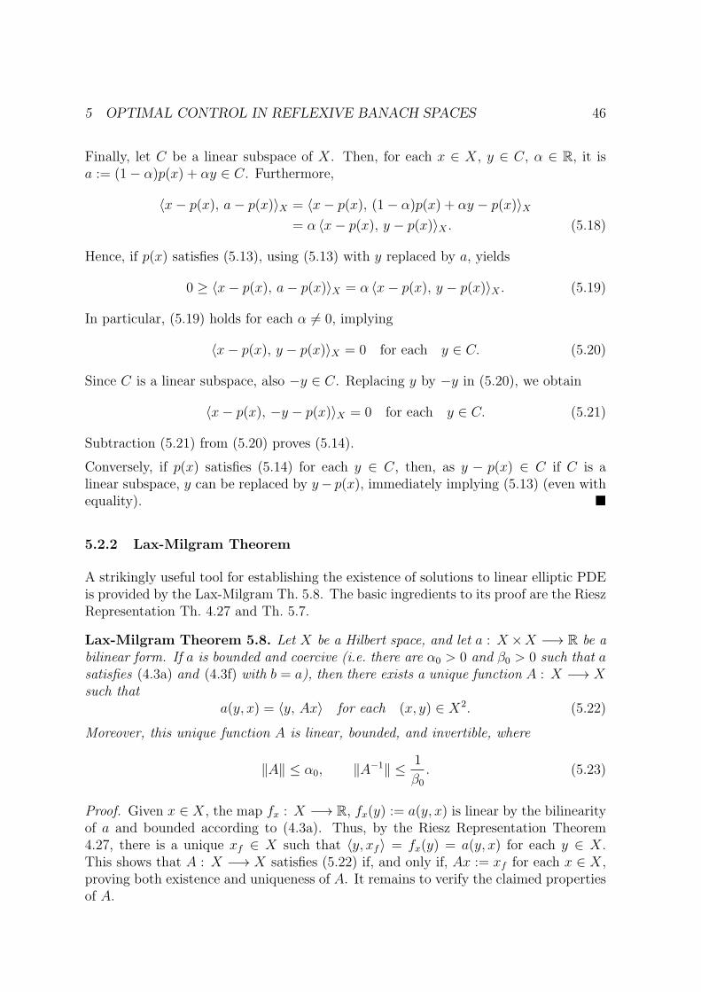
5 OPTIMAL CONTROL IN REFLEXIVE BANACH SPACES 46
Finally, let C be a linear subspace of X. Then, for each x ∈ X, y ∈ C, α ∈ R, it isa := (1− α)p(x) + αy ∈ C. Furthermore,
〈x− p(x), a− p(x)〉X = 〈x− p(x), (1− α)p(x) + αy − p(x)〉X= α 〈x− p(x), y − p(x)〉X . (5.18)
Hence, if p(x) satisfies (5.13), using (5.13) with y replaced by a, yields
0 ≥ 〈x− p(x), a− p(x)〉X = α 〈x− p(x), y − p(x)〉X . (5.19)
In particular, (5.19) holds for each α 6= 0, implying
〈x− p(x), y − p(x)〉X = 0 for each y ∈ C. (5.20)
Since C is a linear subspace, also −y ∈ C. Replacing y by −y in (5.20), we obtain
〈x− p(x), −y − p(x)〉X = 0 for each y ∈ C. (5.21)
Subtraction (5.21) from (5.20) proves (5.14).
Conversely, if p(x) satisfies (5.14) for each y ∈ C, then, as y − p(x) ∈ C if C is alinear subspace, y can be replaced by y− p(x), immediately implying (5.13) (even withequality).
5.2.2 Lax-Milgram Theorem
A strikingly useful tool for establishing the existence of solutions to linear elliptic PDEis provided by the Lax-Milgram Th. 5.8. The basic ingredients to its proof are the RieszRepresentation Th. 4.27 and Th. 5.7.
Lax-Milgram Theorem 5.8. Let X be a Hilbert space, and let a : X ×X −→ R be abilinear form. If a is bounded and coercive (i.e. there are α0 > 0 and β0 > 0 such that asatisfies (4.3a) and (4.3f) with b = a), then there exists a unique function A : X −→ Xsuch that
a(y, x) = 〈y, Ax〉 for each (x, y) ∈ X2. (5.22)
Moreover, this unique function A is linear, bounded, and invertible, where
‖A‖ ≤ α0, ‖A−1‖ ≤ 1
β0
. (5.23)
Proof. Given x ∈ X, the map fx : X −→ R, fx(y) := a(y, x) is linear by the bilinearityof a and bounded according to (4.3a). Thus, by the Riesz Representation Theorem4.27, there is a unique xf ∈ X such that 〈y, xf〉 = fx(y) = a(y, x) for each y ∈ X.This shows that A : X −→ X satisfies (5.22) if, and only if, Ax := xf for each x ∈ X,proving both existence and uniqueness of A. It remains to verify the claimed propertiesof A.
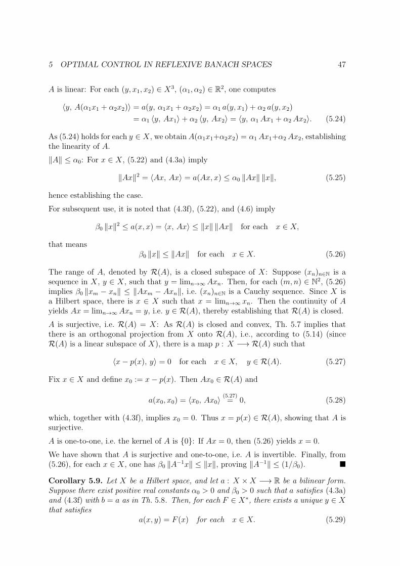
5 OPTIMAL CONTROL IN REFLEXIVE BANACH SPACES 47
A is linear: For each (y, x1, x2) ∈ X3, (α1, α2) ∈ R2, one computes
〈y, A(α1x1 + α2x2)〉 = a(y, α1x1 + α2x2) = α1 a(y, x1) + α2 a(y, x2)
= α1 〈y, Ax1〉+ α2 〈y, Ax2〉 = 〈y, α1Ax1 + α2 Ax2〉. (5.24)
As (5.24) holds for each y ∈ X, we obtainA(α1x1+α2x2) = α1 Ax1+α2 Ax2, establishingthe linearity of A.
‖A‖ ≤ α0: For x ∈ X, (5.22) and (4.3a) imply
‖Ax‖2 = 〈Ax, Ax〉 = a(Ax, x) ≤ α0 ‖Ax‖ ‖x‖, (5.25)
hence establishing the case.
For subsequent use, it is noted that (4.3f), (5.22), and (4.6) imply
β0 ‖x‖2 ≤ a(x, x) = 〈x, Ax〉 ≤ ‖x‖ ‖Ax‖ for each x ∈ X,
that meansβ0 ‖x‖ ≤ ‖Ax‖ for each x ∈ X. (5.26)
The range of A, denoted by R(A), is a closed subspace of X: Suppose (xn)n∈N is asequence in X, y ∈ X, such that y = limn→∞Axn. Then, for each (m,n) ∈ N2, (5.26)implies β0 ‖xm − xn‖ ≤ ‖Axm − Axn‖, i.e. (xn)n∈N is a Cauchy sequence. Since X isa Hilbert space, there is x ∈ X such that x = limn→∞ xn. Then the continuity of Ayields Ax = limn→∞Axn = y, i.e. y ∈ R(A), thereby establishing that R(A) is closed.
A is surjective, i.e. R(A) = X: As R(A) is closed and convex, Th. 5.7 implies thatthere is an orthogonal projection from X onto R(A), i.e., according to (5.14) (sinceR(A) is a linear subspace of X), there is a map p : X −→ R(A) such that
〈x− p(x), y〉 = 0 for each x ∈ X, y ∈ R(A). (5.27)
Fix x ∈ X and define x0 := x− p(x). Then Ax0 ∈ R(A) and
a(x0, x0) = 〈x0, Ax0〉(5.27)= 0, (5.28)
which, together with (4.3f), implies x0 = 0. Thus x = p(x) ∈ R(A), showing that A issurjective.
A is one-to-one, i.e. the kernel of A is 0: If Ax = 0, then (5.26) yields x = 0.
We have shown that A is surjective and one-to-one, i.e. A is invertible. Finally, from(5.26), for each x ∈ X, one has β0 ‖A−1x‖ ≤ ‖x‖, proving ‖A−1‖ ≤ (1/β0).
Corollary 5.9. Let X be a Hilbert space, and let a : X ×X −→ R be a bilinear form.Suppose there exist positive real constants α0 > 0 and β0 > 0 such that a satisfies (4.3a)and (4.3f) with b = a as in Th. 5.8. Then, for each F ∈ X∗, there exists a unique y ∈ Xthat satisfies
a(x, y) = F (x) for each x ∈ X. (5.29)
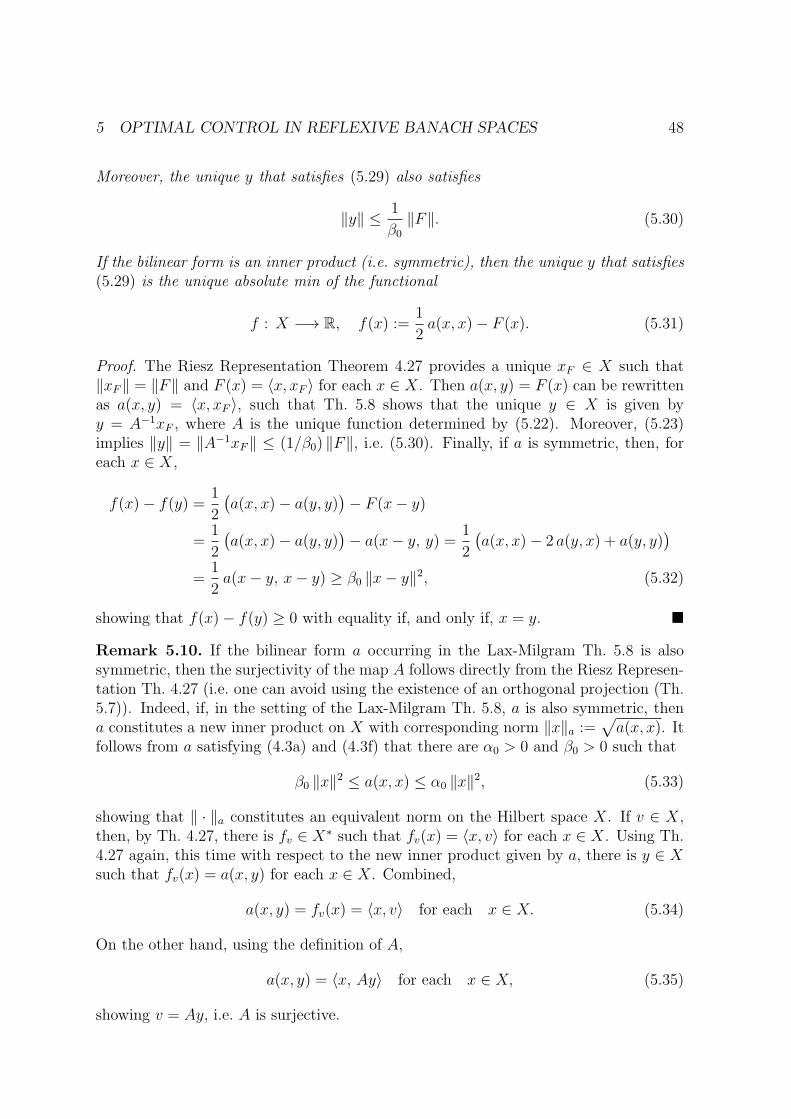
5 OPTIMAL CONTROL IN REFLEXIVE BANACH SPACES 48
Moreover, the unique y that satisfies (5.29) also satisfies
‖y‖ ≤ 1
β0
‖F‖. (5.30)
If the bilinear form is an inner product (i.e. symmetric), then the unique y that satisfies(5.29) is the unique absolute min of the functional
f : X −→ R, f(x) :=1
2a(x, x)− F (x). (5.31)
Proof. The Riesz Representation Theorem 4.27 provides a unique xF ∈ X such that‖xF‖ = ‖F‖ and F (x) = 〈x, xF 〉 for each x ∈ X. Then a(x, y) = F (x) can be rewrittenas a(x, y) = 〈x, xF 〉, such that Th. 5.8 shows that the unique y ∈ X is given byy = A−1xF , where A is the unique function determined by (5.22). Moreover, (5.23)implies ‖y‖ = ‖A−1xF‖ ≤ (1/β0) ‖F‖, i.e. (5.30). Finally, if a is symmetric, then, foreach x ∈ X,
f(x)− f(y) =1
2
(a(x, x)− a(y, y)
)− F (x− y)
=1
2
(a(x, x)− a(y, y)
)− a(x− y, y) =
1
2
(a(x, x)− 2 a(y, x) + a(y, y)
)=
1
2a(x− y, x− y) ≥ β0 ‖x− y‖2, (5.32)
showing that f(x)− f(y) ≥ 0 with equality if, and only if, x = y.
Remark 5.10. If the bilinear form a occurring in the Lax-Milgram Th. 5.8 is alsosymmetric, then the surjectivity of the map A follows directly from the Riesz Represen-tation Th. 4.27 (i.e. one can avoid using the existence of an orthogonal projection (Th.5.7)). Indeed, if, in the setting of the Lax-Milgram Th. 5.8, a is also symmetric, thena constitutes a new inner product on X with corresponding norm ‖x‖a :=
√a(x, x). It
follows from a satisfying (4.3a) and (4.3f) that there are α0 > 0 and β0 > 0 such that
β0 ‖x‖2 ≤ a(x, x) ≤ α0 ‖x‖2, (5.33)
showing that ‖ · ‖a constitutes an equivalent norm on the Hilbert space X. If v ∈ X,then, by Th. 4.27, there is fv ∈ X∗ such that fv(x) = 〈x, v〉 for each x ∈ X. Using Th.4.27 again, this time with respect to the new inner product given by a, there is y ∈ Xsuch that fv(x) = a(x, y) for each x ∈ X. Combined,
a(x, y) = fv(x) = 〈x, v〉 for each x ∈ X. (5.34)
On the other hand, using the definition of A,
a(x, y) = 〈x, Ay〉 for each x ∈ X, (5.35)
showing v = Ay, i.e. A is surjective.
6 OPTIMAL CONTROL OF LINEAR ELLIPTIC PDE 49
6 Optimal Control of Linear Elliptic PDE
6.1 Sobolev Spaces
6.1.1 Lp-Spaces
Notation 6.1. For each m ∈ N, let λm denote m-dimensional Lebesgue measure.
Definition 6.2. Let E be a measurable subset of Rm, m ∈ N. For each p ∈ [1,∞[, letLp(E) denote the set of all measurable functions f : E −→ R such that∫
E
|f(x)|p dx < ∞. (6.1)
For each f ∈ Lp(E) define
‖f‖p :=(∫
E
|f(x)|p dx) 1
p
. (6.2)
Furthermore, define L∞(E) to be the set consisting of all measurable functions f :E −→ R such that
‖f‖∞ := inf
sup
|f(x)| : x ∈ E \N
: N measurable and λm(N) = 0
< ∞. (6.3)
The number defined in (6.3) is also known as the essential supremum of f . In the usualway, we define equivalence relations on the spaces Lp(E), p ∈ [1,∞], by consideringfunctions as equivalent if they only differ on sets of measure zero. The respective sets ofequivalence classes are denoted by Lp(E). A certain sloppiness is quite common in thatone often does not properly distinguish between elements of Lp(E) and Lp(E). Thissloppiness does not lead to confusion in most cases and it will occasionally be presentbelow.
Riesz-Fischer Theorem 6.3. For each measurable E ⊆ Rm and each p ∈ [1,∞],the space
(Lp(E), ‖ · ‖p
)is a Banach space (whereas the Lp(E) are merely seminormed
spaces, which is the main reason for working with Lp(E)).
Proof. See, e.g., [Roy88, Ch. 11, Th. 25, Ch. 6, Th. 6] or [Els96, Ch. VI, Th. 2.5].
Holder Inequality 6.4. Let E ⊆ Rm be measurable, (p, q) ∈ [1,∞]2 such that 1/p +1/q = 1. If f ∈ Lp(E), g ∈ Lq(E), then f g ∈ L1(E) and∫
E
|f g| ≤ ‖f‖p ‖g‖q. (6.4)
Proof. See, e.g., [Roy88, Ch. 11, Th. 25, Ch. 6, Th. 4] or [Els96, Ch. VI, Th. 1.5].
6 OPTIMAL CONTROL OF LINEAR ELLIPTIC PDE 50
Remark 6.5. Observing that, for each measurable E ⊆ Rm, the map (f, g) 7→∫Ef g,
defines an inner product on L2(E) (note that f g ∈ L1(E) for f, g ∈ L2(E) by theHolder Ineq. 6.4), Th. 6.3 implies that L2(E) is a Hilbert space.
Riesz Representation Theorem 6.6. For each measurable E ⊆ Rm and each p ∈[1,∞[, one has (Lp(E))∗ = Lq(E) (1/p + 1/q = 1) in the sense that, for each boundedlinear functional F on Lp(E), there exists a unique g ∈ Lq(E) satisfying
F (f) =
∫E
f g for each f ∈ Lp(E), (6.5)
and, moreover, ‖F‖ = ‖g‖q. In particular, for 1 < p < ∞, Lp(E) is reflexive.
Proof. See, e.g., [Roy88, Ch. 11, Th. 29, Ch. 6, Th. 13] or [Els96, Ch. VII, Th. 3.2].
Remark 6.7. As a caveat, it is remarked that, in general, even though (L1(E))∗ =L∞(E), one has (L∞(E))∗ 6= L1(E), implying that L1(E) is not reflexive. See [Yos74,Ex. IV.9.5] for a representation of (L∞(E))∗.
Definition 6.8. Given E ⊆ Rm measurable and a measurable f : E −→ R, f is calledintegrable if, and only if, f ∈ L1(E). Moreover, f is called locally integrable if, and onlyif, for each compact K ⊆ E, the restriction of f to K is in L1(K), i.e. f is integrableover every compact subset of E. The set of all locally integrable functions on E isdenoted by L1
loc(E).
6.1.2 Weak Derivatives
Definition 6.9. The support of a function f : Ω −→ R defined on a set Ω ⊆ Rm,denoted supp(f), is the closure of the set of points, where f does not vanish, i.e.
supp(f) := x ∈ Ω : f(x) 6= 0 ⊆ Ω. (6.6)
Notation 6.10. Let Ω ⊆ Rm be open, and let k ∈ N0.
(a) Let Ck(Ω) denote the set of all functions f : Ω −→ R such that f has continuouspartial derivatives up to order k (i.e. including those of order k). One also says thatfunctions in Ck(Ω) are of class Ck. Set C(Ω) := C0(Ω) and C∞(Ω) :=
⋂k∈N0
Ck(Ω).
(b) Let Ck(Ω) denote the set of all functions from Ck(Ω) such that all their partialderivatives up to order k extend continuously to Ω. Set C(Ω) := C0(Ω) andC∞(Ω) :=
⋂k∈N0
Ck(Ω).
(c) Let Ck0 (Ω) denote the set of all functions f from Ck(Ω) that have a compact support
contained in Ω, i.e. supp(f) ⊆ Ω. Set C0(Ω) := C00(Ω) and C∞
0 (Ω) :=⋂
k∈N0Ck
0 (Ω).

6 OPTIMAL CONTROL OF LINEAR ELLIPTIC PDE 51
Remark 6.11. The elements φ ∈ C∞0 (Ω) have numerous particularly benign and use-
ful properties that are subsequently exploited when defining weak derivatives. Theseproperties include the fact that φf is integrable for each f ∈ L1
loc(Ω), φ satisfies thesimplified integration by parts formula (6.11), and φ can be differentiated as often asneeded. Fortunately, elements of φ ∈ C∞
0 (Ω) are also very abundant as can be seenfrom the next theorem.
Theorem 6.12. If Ω ⊆ Rm is open and p ∈ [1,∞[, then C∞0 (Ω) is dense in Lp(Ω), i.e.
Lp(Ω) is the closure of C∞0 (Ω) with respect to ‖ · ‖p.
Proof. See [Alt06, Th. 2.14〈3〉].
Fundamental Lemma of Variational Calculus 6.13. If Ω ⊆ Rm is open and f ∈L1loc(Ω), then ∫
Ω
f φ = 0 for each φ ∈ C∞0 (Ω) (6.7)
implies that f = 0 almost everywhere.
Proof. See [Zei90, Prop. 18.36].
Notation 6.14. A multi-index α is a finite sequence of nonnegative integers, i.e. α =(α1, . . . , αm) ∈ Nm
0 , m ∈ N, where |α| := α1 + · · · + αm is called the order of α. Ifα = (α1, . . . , αm) is a multi-index, Ω ⊆ Rm is open, and f ∈ Ck(Ω), where k = |α|,then Dαf denotes a partial derivative of f of order k, namely
Dαf :=
(m∏i=1
∂αii
)f = ∂α1
1 · · · ∂αmm f, (6.8)
where ∂0i f := f . Thus, for example, if α = (1, 0, 2), then Dαf = ∂1∂3∂3f .
Remark 6.15. Note that the definition in (6.8) is biased with respect to the orderof partial derivatives (partial derivatives with respect to the mth variable are alwayscarried out first). Of course, for functions of class Ck, partial derivatives commute andthis bias is of no consequence.
Remark 6.16. For Ω ⊆ Rm open and bounded, k ∈ N0, and f ∈ Ck(Ω), let
‖f‖Ck(Ω) := maxx∈Ω
∑α∈Nm
0 : |α|≤k
|Dαf(x)|. (6.9)
The numbers ‖f‖Ck(Ω) are well-defined as each of the continuous functions |Dαf | as-sumes its maximum on the compact set Ω. Moreover, ‖·‖Ck(Ω) defines a norm on Ck(Ω)
that makes Ck(Ω) into a Banach space.
Remark 6.17. Let Ω ⊆ Rm be open. If f, g ∈ C1(Ω) and f or g is in C10(Ω), then the
following integration by parts formula holds:∫Ω
g ∂if = −∫Ω
f ∂ig for each i ∈ 1, . . . ,m. (6.10)
6 OPTIMAL CONTROL OF LINEAR ELLIPTIC PDE 52
To verify (6.10), one first uses the Fubini theorem to show
φ ∈ C10(Ω) ⇒
∫Rm
∂iφ = 0 for each i ∈ 1, . . . ,m. (6.11)
Then this implies (6.10) for Ω = Rm, which, in turn, extends to general open Ω vianoticing that fg has compact support inside Ω, i.e. extending fg by 0 yields an elementof C1
0(Rm).
—
One now uses (6.10) to define derivatives (so-called weak derivatives) for a larger classof locally integrable functions.
Definition 6.18. Let Ω ⊆ Rm be open. If f ∈ L1loc(Ω) and α ∈ Nm
0 is a multi-index,then a function g ∈ L1
loc(Ω) is called a weak derivative with respect to α if, and only if,∫Ω
f ∂αφ = (−1)|α|∫Ω
g φ for each φ ∈ C∞0 (Ω). (6.12)
If (6.12) holds, then we will also write Dαf instead of g. The following Rem. 6.19provides a justification for this notation.
Remark 6.19. Weak derivatives are unique: If g1 and g2 are weak derivatives of fwith respect to α, then (6.12) implies
∫Ω(g1 − g2)φ = 0 for each φ ∈ C∞
0 (Ω), yieldingg1 = g2 by Th. 6.13. The uniqueness of weak derivatives together with the integrationby parts formula in Rem. 6.17 shows that the weak derivative Dαf coincides with thecorresponding classical partial derivative of f provided that f ∈ Ck(Ω), where k := |α|.As a caveat, it is noted that, if f does not have continuous partials up to order k, thenthe weak derivatives can not be guaranteed to agree with the classical derivatives (see[Rud73, Ex. 6.14] for examples). Here, in such cases, Dαf will always mean the weakderivative of f .
Definition 6.20. Let Ω ⊆ Rm be open, (k, p) ∈ N0 × [1,∞]. By W k,p(Ω) we denotethe subset of L1
loc(Ω) consisting of all functions f such that the weak derivatives Dαfexist and lie in Lp(Ω) for each multi-index α with |α| ≤ k. The spaces W k,p(Ω) arereferred to as Sobolev spaces. The case p = 2 is of particular interest, and one setsHk(Ω) := W k,2(Ω). Furthermore, for each f ∈ W k,p(Ω), p < ∞, define
‖f‖Wk,p(Ω) :=
∑α∈Nm
0 : |α|≤k
∫Ω
|Dαf |p 1
p
=
∑α∈Nm
0 : |α|≤k
‖Dαf‖pp
1p
, (6.13a)
and, for each f ∈ W k,∞(Ω),
‖f‖Wk,∞(Ω) := max‖Dαf‖∞ : α ∈ Nm
0 , |α| ≤ k. (6.13b)

6 OPTIMAL CONTROL OF LINEAR ELLIPTIC PDE 53
Theorem 6.21. Let Ω ⊆ Rm be open. For each (k, p) ∈ N0 × [1,∞], the Sobolev spaceW k,p(Ω) is a Banach space. In particular, each Hk(Ω) = W k,2(Ω) is a Hilbert spacewith respect to the inner product
〈f, g〉Hk(Ω) =∑
α∈Nm0 : |α|≤k
∫Ω
Dαf Dαg =∑
α∈Nm0 : |α|≤k
〈Dαf,Dαg〉L2(Ω). (6.14)
Proof. See, e.g., [Alt06, p. 64] or [RR96, Th. 6.65]. The case p < ∞ is also treated in[Yos74, Prop. I.9.5].
Definition 6.22. Let Ω ⊆ Rm be open. For each (k, p) ∈ N0 × [1,∞], let W k,p0 (Ω)
denote the closure of the set C∞0 (Ω) in W k,p(Ω), i.e. the closure of C∞
0 (Ω) with respectto the ‖ · ‖Wk,p(Ω)-norm; let Hk
0 (Ω) := W k,20 (Ω).
Remark 6.23. As closed subspaces of Banach spaces, the W k,p0 (Ω) are themselves
Banach spaces for each open Ω ⊆ Rm and each (k, p) ∈ N0 × [1,∞]; the Hk0 (Ω) are
Hilbert spaces.
Poincare-Friedrich Inequality 6.24. Let Ω ⊆ Rm be open and bounded. Then thereexists an Ω-dependent constant cΩ > 0 such that
‖f‖2L2(Ω) =
∫Ω
|f |2 ≤ cΩ
∫Ω
| ∇ f |2 = cΩ
∫Ω
m∑i=1
|∂if |2 for each f ∈ H10 (Ω). (6.15)
Proof. See, e.g., [Alt06, 4.7] or [RR96, Th. 6.101].
6.1.3 Boundary Issues
Our main goal is the solution and control of PDE. We will see in Sec. 6.2 that solutionsof PDE are typically found as elements of Sobolev spaces. On the other hand, as wasalready seen in the motivating examples of Sec. 1, suitable boundary conditions arean essential part of PDE. Thus, if one is to consider PDE on some open set Ω ⊆ Rm,then one needs a workable notion of restriction (or trace) of elements of Sobolev spaces(i.e. of weakly differentiable functions) with respect to ∂Ω. A problem arises from thefact that W k,p(Ω) consists of equivalence classes of functions that only differ on setsof measure zero (with respect to λm) and λm(∂Ω) = 0. Thus, if f ∈ W k,p(Ω), thendifferent functions representing f will, in general, have different restrictions on ∂Ω, andusing representatives to define a restriction (or trace) of f is not feasible. On the otherhand, continuous functions f ∈ C(Ω) do have a well-defined restriction on ∂Ω, andit turns out that this can be used to define a useful notion of restriction (or trace) ofweakly differentiable functions (see Th. 6.35).
In a related issue, one has to address the regularity of ∂Ω. For general open sets Ω,the boundary can be extremely pathological. On the other hand, requiring ∂Ω tobe smooth (e.g. of class C1) seems too restrictive, as surfaces with corners occur innumerous applications. As it turns out, the notion of a Lipschitz boundary (Def. 6.27,
6 OPTIMAL CONTROL OF LINEAR ELLIPTIC PDE 54
cf. [Alt06, Sec. A6.2], [Tro05, Sec. 2.2.2], [Wlo82, Def. 2.4]) constitutes an effectivecompromise. Moreover, we will restrict ourselves to the case, where Ω is bounded.
Roughly, a bounded open set Ω ⊆ Rm has a Lipschitz boundary if, and only if, theboundary is locally representable as the graph of Lipschitz functions, where Ω lies ononly one side of that graph. The technical definition is somewhat tedious and needssome preparation.
Remark 6.25. The case that Ω is an open bounded subset of R is particularly sim-ple. However, the fact that ∂Ω is 0-dimensional requires some special treatment anddefinitions. As in [Tro05], we will avoid this issue by stating subsequent definitions andresults only for Ω ⊆ Rm with m ≥ 2. With the appropriate modifications, the casem = 1 is usually much simpler to treat. For example, a bounded open set Ω ⊆ R hasa Lipschitz boundary if, and only if, it consists of finitely many open intervals havingpositive distance from each other.
Definition 6.26. Let Ω ⊆ Rm, m ∈ N. A map f : Ω −→ R is called Lipschitzcontinuous if, and only if, there exists L ∈ R+
0 , such that, for each (x, y) ∈ Ω, |f(x) −f(y)| ≤ L |x− y|, recalling that we use | · | to denote the Euclidian norm. The set of allLipschitz continuous maps on Ω is denoted by C0,1(Ω).
—
We will now state the definition of a set with Lipschitz boundary, followed by somefurther explanation directly after the definition.
Definition 6.27. Let Ω ⊆ Rm, m ≥ 2, be open and bounded. Then Ω is said to have aLipschitz boundary if, and only if, there are finitely many open subsets of Rm, denoted byU1, . . . , UM , M ∈ N, rotations ρj : Rm −→ Rm, reference points yj = (yj1, . . . , y
jm−1) ∈
Rm−1, and Lipschitz continuous functions hj : Rm−1 −→ R, j ∈ 1, . . . ,M, as wellas positive real numbers a > 0, b > 0, such that the following conditions (i) – (iii) aresatisfied:
(i) ∂Ω ⊆⋃M
j=1 Uj.
(ii) For each j ∈ 1, . . . ,M:
Uj = ρj
((x1, . . . , xm) : |yj − (x1, . . . , xm−1)| < a, |xm − hj(y
j)| < b)
.
(iii) For each j ∈ 1, . . . ,M:
Uj ∩ ∂Ω = ρj
((y, hj(y)) : |yj − y| < a
), (6.16a)
Uj ∩ Ω = ρj
((y, xm) : |yj − y| < a, hj(y) < xm < hj(y) + b
), (6.16b)
Uj \ Ω = ρj
((y, xm) : |yj − y| < a, hj(y)− b < xm < hj(y)
). (6.16c)
—
6 OPTIMAL CONTROL OF LINEAR ELLIPTIC PDE 55
The rotations ρj in Def. 6.27 are needed as, in general, some parts of ∂Ω are perpen-dicular to the (m− 1)-dimensional hyperplane H := Rm−1 ×0 ⊆ Rm. However, afterrotating H by applying ρj, no part of the small patch Uj ∩ ∂Ω is perpendicular to theresulting hyperplane, i.e. to ρj(H). Moreover, shifting Uj ∩ ∂Ω for a small distance inthe direction perpendicular to ρj(H) either results in moving Uj ∩ ∂Ω entirely inside ofΩ (cf. (6.16b)) or entirely outside of Ω (cf. (6.16c)), i.e., locally, Ω lies only on one sideof Uj∩∂Ω. Moreover, a neighborhood Nj of y
j ∈ H can be deformed into Uj∩∂Ω usinghj in the sense that, after applying the rotation to the deformed piece, the resulting setis identical to Uj ∩ ∂Ω (cf. (6.16a)).
Theorem 6.28. Let the bounded and open set Ω ⊆ Rm be a set with Lipschitz boundary.Then the identity map provides an isomorphism between C0,1(Ω) and W 1,∞(Ω):
Id : C0,1(Ω) ∼= W 1,∞(Ω). (6.17)
More precisely, each f ∈ C0,1(Ω) represents an equivalence class that is an element ofW 1,∞(Ω) and each element of W 1,∞(Ω) contains precisely one representative that liesin C0,1(Ω).
Proof. See [Alt06, Th. 8.5〈2〉]. The case where ∂Ω is of class C1 is also treated in[Eva98, Sec. 5.8, Th. 4–6].
Theorem 6.29. Let the bounded and open set Ω ⊆ Rm be a set with Lipschitz boundary.Then, for each 1 ≤ p < ∞ and each k ∈ N0, C
∞(Ω) is dense in W k,p(Ω).
Proof. See, e.g., [Alt06, Lem. A6.7] or (for the case p = 2) [Zei90, Cor. 21.15(a)].
Before formulating a boundary trace theorem for functions inW 1,p(Ω), we need to definethe space L2(∂Ω) or, more generally, Lp-spaces of functions living on ∂Ω. In particular,we need to define a suitable measure on ∂Ω, the so-called surface measure. The strategyfor that is, given some x ∈ ∂Ω, to first work in a local neighborhood of x (such as thesets Uj ∩ ∂Ω given by Def. 6.27), and then to patch everything together using a so-called partition of unity. Finally, one needs to show that the resulting definitions donot depend on the choice of local coordinates and the choice of partition of unity. Thefollowing Def. 6.31 of a partition of unity is tailored for our purposes. In the literature,one typically finds more general and sometimes slightly modified notions of partitionsof unity (see, e.g., [Alt06, 2.19], [Wlo82, Sec. 1.2]).
Definition 6.30. Let A ⊆ Rm, m ∈ N. A finite family (O1, . . . , ON), N ∈ N, of opensets Oi ⊆ Rm is called a finite open cover of A if, and only if, A ⊆
⋃Ni=1 Oi.
Definition 6.31. Let A ⊆ Rm, m ∈ N. Given a finite open cover O = (O1, . . . , ON),N ∈ N, of A, a family of functions (η1, . . . , ηN), ηi ∈ C∞
0 (Rm), is called a partition ofunity subordinate to O if, and only if, 0 ≤ ηi ≤ 1, supp(ηi) ⊆ Oi for each i ∈ 1, . . . , N,and
N∑i=1
ηi(x) = 1 for each x ∈ A. (6.18)
6 OPTIMAL CONTROL OF LINEAR ELLIPTIC PDE 56
Partition of Unity Theorem 6.32. Let A ⊆ Rm, m ∈ N. Given a finite open coverO = (O1, . . . , ON), N ∈ N, of A, there exists a partition of unity subordinate to O.
Proof. See [Alt06, 2.19〈3〉].
Definition and Remark 6.33. Let the bounded and open set Ω ⊆ Rm be a setwith Lipschitz boundary, m ≥ 2. Let U1, . . . , UM , M ∈ N, ρj : Rm −→ Rm, yj =(yj1, . . . , y
jm−1) ∈ Rm−1, hj : Rm−1 −→ R, j ∈ 1, . . . ,M, and a > 0, b > 0 be as in
Def. 6.27. Let U0 := Ω. Then, according to Def. 6.27(i), (U1, . . . , UM) forms a finiteopen cover of ∂Ω and O := (U0, . . . , UM) forms a finite open cover of Ω. Thus, by Th.6.32, we can choose a partition of unity (η0, . . . , ηM) subordinate to O.
(a) A function f : ∂Ω −→ R is called λm−1-measurable (respectively λm−1-integrable)if, and only if, for each j ∈ 1, . . . ,m, the function
fj : Rm−1 −→ R, fj(y) :=
(ηjf)
(ρj(y, hj(y)
))for y ∈ Ba(y
j),
0 for y ∈ Rm−1 \Ba(yj)
(6.19)is measurable (respectively integrable) in the usual sense. If f : ∂Ω −→ R isintegrable or nonnegative and measurable, then define∫
∂Ω
f dλm−1 :=M∑j=1
∫Rm−1
fj(y)√
1 + |∇hj(y)|2 dy , (6.20)
where it is noted that, as hj : Rm−1 −→ R is presumed to be Lipschitz continuous,hjBa(yj)∈ W 1,∞(Ba(y
j)) according to (6.17).
Now, given A ⊆ ∂Ω, call A λm−1-measurable if, and only if, the characteristicfunction 1A : ∂Ω −→ 0, 1 is λm−1-measurable. If A is λm−1-measurable, thendefine
λm−1(A) :=
∫∂Ω
1A dλm−1 . (6.21)
Then λm−1 defines, indeed, a measure on ∂Ω, called the surface measure. Moreover,the integral defined in (6.20) coincides with the integral with respect to the surfacemeasure, thereby justifying the notation
∫∂Ω
f dλm−1 .
(b) For each p ∈ [1,∞[, let Lp(∂Ω) denote the set of all λm−1-measurable functionsf : ∂Ω −→ R such that ∫
∂Ω
|f |p dλm−1 < ∞. (6.22)
For each f ∈ Lp(∂Ω) define
‖f‖p :=(∫
∂Ω
|f |p dλm−1
) 1p
. (6.23)
6 OPTIMAL CONTROL OF LINEAR ELLIPTIC PDE 57
Furthermore, define L∞(∂Ω) to be the set consisting of all λm−1-measurable func-tions f : ∂Ω −→ R such that
‖f‖∞ := inf
sup
|f(x)| : x ∈ (∂Ω) \N
:
N λm−1-measurable and λm−1(N) = 0
< ∞.
(6.24)
Analogous to the λm-case, we define equivalence relations on the spaces Lp(∂Ω),p ∈ [1,∞], by considering functions as equivalent if they only differ on sets of λm−1-measure zero. The respective sets of equivalence classes are denoted by Lp(∂Ω).Also analogous to the λm-case, it is quite common to permit a certain sloppiness,not always properly distinguishing between elements of Lp(∂Ω) and Lp(∂Ω).
(c) We define a functionν : ∂Ω −→ Rm, (6.25)
called the outer unit normal to Ω, as well as functions
τk : ∂Ω −→ Rm for each k ∈ 1, . . . ,m− 1, (6.26)
called unit tangent vectors to Ω, as follows: Given x ∈ ∂Ω, there is j ∈ 1, . . . ,Msuch that x ∈ Uj ∩ ∂Ω. If x ∈ Uj ∩ ∂Ω, then, according to (6.16b), there isyx ∈ Ba(y
j) such thatx = ρj
(yx, hj(yx)
). (6.27)
Again recalling that hjBa(yj)∈ W 1,∞(Ba(yj)), we define
ν(x) :=(1 + |∇hj(yx)|2
)− 12 ρj(∇hj(yx), −1
), (6.28)
and
τk(x) :=(1 +
(∂khj(yx)
)2)− 12ρj(τ 0(x)
)for each k ∈ 1, . . . ,m− 1, (6.29)
where
τ 0k,i(x) :=
1 for i = k,
∂khj(yx) for i = m,
0 for i ∈ 1, . . . ,m \ k,m.(6.30)
Theorem 6.34. Let the bounded and open set Ω ⊆ Rm be a set with Lipschitz boundary,m ≥ 2. Then the surface measure λm−1 on ∂Ω, the measurability, the integrability, andthe integrals with respect to λm−1, as well as the spaces Lp(∂Ω) and Lp(∂Ω), p ∈ [1,∞],the normal vector ν and the tangent space spanτ1, . . . , τm−1 to Ω spanned by thetangent vectors, all defined in Def. and Rem. 6.33, are independent of the chosen setsU1, . . . , UM , M ∈ N, ρj : Rm −→ Rm, yj = (yj1, . . . , y
jm−1) ∈ Rm−1, hj : Rm−1 −→ R,
j ∈ 1, . . . ,M, as well as independent of the chosen partition of unity (η0, . . . , ηM).Note that the individual tangent vectors τ1, . . . , τm−1 do depend on the choice of localcoordinates hj and ρj.

6 OPTIMAL CONTROL OF LINEAR ELLIPTIC PDE 58
Moreover, Lp(∂Ω) is a Banach space for each p ∈ [1,∞]. The outer unit normalν : ∂Ω −→ Rm and the unit tangent vectors τk : ∂Ω −→ Rm, k ∈ 1, . . . ,m− 1, havethe following properties: All components are bounded λm−1-measurable functions, i.e.νi ∈ L∞(∂Ω) and τk,i ∈ L∞(∂Ω) for each i ∈ 1, . . . ,m. Moreover, the vectors are,indeed, unit vectors, i.e. |ν| ≡ 1 and |τk| ≡ 1. For λm−1-almost every x ∈ ∂Ω (moreprecisely, using the notation from Def. and Rem. 6.33(c), for every x = ρj
(yx, hj(yx)
)∈
∂Ω such that hj is differentiable in yx ∈ Ba(yj)), ν(x) is perpendicular to each τk(x),
i.e. ⟨ν(x), τk(x)
⟩Rm = 0 for each k ∈ 1, . . . ,m− 1; (6.31)
and ν(x) is pointing outwards, i.e. there is ε0 > 0 such that x + εν(x) 6∈ Ω for each0 ≤ ε < ε0.
Proof. See [Alt06, A.6.5〈1〉–〈3〉].
Theorem 6.35. Let the bounded and open set Ω ⊆ Rm be a set with Lipschitz boundary.Then, for each 1 ≤ p ≤ ∞, there is a unique bounded linear map τ : W 1,p(Ω) −→Lp(∂Ω), called the trace operator, such that, for each f ∈ C0(Ω) ∩ W 1,p(Ω), one hasτf = f ∂Ω, where f ∂Ω denotes the restriction of f to ∂Ω. The function τf is calledthe trace of f on ∂Ω. Moreover, the trace operator is positive, i.e. if f ≥ 0 λm-almosteverywhere on Ω, then τf ≥ 0 λm−1-almost everywhere on ∂Ω.
Proof. See, e.g., [Alt06, Lem. A6.6] or (for the case p = 2) [Zei90, Th. 21.A(e)]. Thepositivity of the trace operator follows by noting that, when proving Th. 6.29, forf ∈ W 1,p(Ω) and f ≥ 0, one can choose the approximating functions fn ∈ C∞(Ω) tobe nonnegative as well (cf. [KS80, Prop. 5.2(ii)]). As τfn ≥ 0, the continuity of τ thenyields τf ≥ 0.
Theorem 6.36. Let the bounded and open set Ω ⊆ Rm be a set with Lipschitz boundary.Then, for each 1 ≤ p ≤ ∞,
W 1,p0 (Ω) =
f ∈ W 1,p(Ω) : τf = 0
. (6.32)
Proof. The case p < ∞ is treated in [Alt06, Lem. A6.10]. The case p = ∞ follows fromTh. 6.28.
6.2 Linear Elliptic PDE
6.2.1 Setting and Basic Definitions, Strong and Weak Formulation
Definition 6.37. An (m × m)-matrix (aij)(i,j)∈1,...,m2 of measurable functions aij :Ω −→ R defined on a measurable set Ω ⊆ Rm is called uniformly elliptic if, and onlyif, there exists α0 ∈ R+ such that
m∑i,j=1
aij(x) ξi ξj ≥ α0 |ξ|2 for each ξ ∈ Rm and each x ∈ Ω. (6.33)
6 OPTIMAL CONTROL OF LINEAR ELLIPTIC PDE 59
It is called almost uniformly elliptic if, and only if, there exists α0 ∈ R+ such that (6.33)holds for almost every x ∈ Ω.
Definition 6.38. Let Ω ⊆ Rm be bounded and open, m ≥ 2. Given hi ∈ C1(Ω), auniformly elliptic (m×m)-matrix of functions (aij)(i,j)∈1,...,m2 , each aij ∈ C1(Ω), g, b ∈C0(Ω), b ≥ 0, we call the following equations (6.34) for the unknown y ∈ C2(Ω)∩C0(Ω),
−m∑i=1
∂i
(m∑j=1
aij∂jy + hi
)+ by = g on Ω, (6.34a)
y = 0 on ∂Ω, (6.34b)
the corresponding elliptic boundary value problem (BVP) on Ω in strong form witha homogeneous Dirichlet condition on the boundary. A function y ∈ C2(Ω) ∩ C0(Ω)satisfying (6.34) is called a strong or classical solution to the problem.
Example 6.39. Let Ω ⊆ Rm be bounded and open as before. In the motivatingexamples of Sec. 1, we considered the heat equation
− div(κ ∇ y) = g on Ω. (6.35)
The left-hand side can be written as
− div(κ ∇ y) = −m∑i=1
∂i(κ ∂iy), (6.36)
such that (6.35) corresponds to (6.34a) with b = 0, hi = 0, aii = κ, aij = 0 for i 6= j,(i, j) ∈ 1, . . . ,m2. For this choice of the aij, if ξ ∈ Rm, then
m∑i,j=1
aij ξi ξj = κ |ξ|2. (6.37)
In particular, (aij)(i,j)∈1,...,m2 is uniformly elliptic if, and only if, the function κ : Ω −→R is measurable and bounded away from 0 by α0 > 0. It is almost uniformly elliptic if,and only if, κ is measurable and κ(x) ≥ α0 for almost every x ∈ Ω.
Remark 6.40. If (6.34b) in Def. 6.38 is replaced with “y = y0 on ∂Ω” with some0 6= y0 ∈ C0(∂Ω), then one speaks of a nonhomogeneous Dirichlet condition. Here, forsimplicity, we will restrict ourselves to homogeneous Dirichlet conditions. Optimal con-trol of PDE with nonhomogeneous Dirichlet conditions involve some special difficulties(see, e.g., [Lio71, Sec. II.4.2]).
Lemma 6.41. In the setting of Def. 6.38, y ∈ C2(Ω) satisfies (6.34a) if, and only if,∫Ω
(m∑i=1
(∂iv)
(m∑j=1
aij∂jy + hi
)+ v (by − g)
)dλm = 0 for each v ∈ C∞
0 (Ω).
(6.38)
6 OPTIMAL CONTROL OF LINEAR ELLIPTIC PDE 60
Proof. Suppose y ∈ C2(Ω) satisfies (6.34a). Multiplying (6.34a) by v ∈ C∞0 (Ω) and
integrating the result over Ω yields
0 = −∫Ω
v
(m∑i=1
∂i
(m∑j=1
aij∂jy + hi
)+ by − g
)dλm . (6.39)
As v ∈ C∞0 (Ω) implies v ∈ C1
0(Ω) and the hypotheses on the aij, hi, and y imply that(∑m
j=1 aij∂jy + hi) ∈ C1(Ω), the integration by parts formula (6.10) applies, and oneobtains (6.38).
Conversely, if y ∈ C2(Ω) satisfies (6.38) for each v ∈ C∞0 (Ω), then the integration
by parts formula (6.10) yields that y satisfies (6.39) for each v ∈ C∞0 (Ω). Applying
the Fundamental Lemma of Variational Calculus 6.13, one obtains that the equationin (6.34a) holds for almost every x ∈ Ω. As the hypotheses imply that both sides of(6.34a) are a continuous function on Ω, it follows that the equation in (6.34a) actuallyholds everywhere in Ω.
Using (6.38), we now proceed to formulate the weak form of (6.34) in Def. 6.42 below.The key observation is that (6.38) makes sense if the differentiability and continuityconditions occurring in Def. 6.38 for the functions hi, aij, g, and b are replaced bysuitable integrability and boundedness conditions (see Def. 6.42), and, in that case, itis no longer necessary to require y ∈ C2(Ω) ∩ C0(Ω), but it suffices to demand that ybe weakly differentiable, i.e. y ∈ H1(Ω). If Ω is a set with Lipschitz boundary (see Def.6.27), then the homogeneous Dirichlet condition (6.34b) can be incorporated into theweak formulation by requiring y ∈ H1
0 (Ω). For our subsequent considerations, the weakformulation will turn out to provide the appropriate setting.
Definition 6.42. Let the bounded and open set Ω ⊆ Rm be a set with Lipschitzboundary, m ≥ 2. Given hi ∈ L2(Ω), an almost uniformly elliptic (m ×m)-matrix offunctions (aij)(i,j)∈1,...,m2 , each aij ∈ L∞(Ω), g ∈ L2(Ω), b ∈ L∞(Ω), b ≥ 0 almosteverywhere, we call the following equation (6.40) for the unknown y ∈ H1
0 (Ω),∫Ω
(m∑i=1
(∂iv)
(m∑j=1
aij∂jy + hi
)+ v (by − g)
)dλm = 0 for each v ∈ H1
0 (Ω),
(6.40)
the corresponding elliptic boundary value problem (BVP) on Ω in weak form with ahomogeneous Dirichlet condition on the boundary. A function y ∈ H1
0 (Ω) satisfying(6.40) is called a weak solution to the problem.
6.2.2 Existence and Uniqueness of Weak Solutions
Theorem 6.43. Let the bounded and open set Ω ⊆ Rm be a set with Lipschitz boundary,m ≥ 2. Given hi ∈ L2(Ω), aij ∈ L∞(Ω), (i, j) ∈ 1, . . . ,m2, g ∈ L2(Ω), b ∈ L∞(Ω),b ≥ 0 almost everywhere, the corresponding elliptic BVP on Ω in weak form with a
6 OPTIMAL CONTROL OF LINEAR ELLIPTIC PDE 61
homogeneous Dirichlet condition on the boundary has a unique weak solution y ∈ H10 (Ω).
More precisely, if (aij)(i,j)∈1,...,m2 is almost uniformly elliptic, satisfying (6.33) withα0 > 0, then there is a unique y ∈ H1
0 (Ω) satisfying (6.40), and, moreover,
‖y‖H1(Ω) ≤ C max(
‖g‖L2(Ω)
∪‖hi‖L2(Ω) : i ∈ 1, . . . ,m
), (6.41)
where C ∈ R+ is the constant defined in (6.52) below.
Keeping the hi, aij, and b fixed with hi = 0 for each i ∈ 1, . . . ,m, the solution operator
S : L2(Ω) −→ H10 (Ω), g 7→ y, (6.42)
is a bounded linear operator that is one-to-one. Furthermore, S is also a bounded linearoperator when interpreted as a map S : L2(Ω) −→ L2(Ω).
Proof. With the intention of applying Cor. 5.9, we define a bilinear form a and inves-tigate its properties.
Claim 1. Under the hypotheses of Th. 6.43, the map
a : H10 (Ω)×H1
0 (Ω) −→ R, a(u, v) :=m∑
i,j=1
∫Ω
(∂iu) aij∂jv dλm +
∫Ω
u b v dλm , (6.43)
defines a bounded and coercive bilinear form.
Proof. Note that a is well-defined: If u, v ∈ H1(Ω), then u, v, ∂iu, and ∂jv all are inL2(Ω). Since aij ∈ L∞(Ω) and b ∈ L∞(Ω), one has aij∂jv ∈ L2(Ω) and bv ∈ L2(Ω).Then (∂iu) aij∂jv ∈ L1(Ω) and u b v ∈ L1(Ω) such that all the integrals in (6.43) existas real numbers.
The bilinearity of a is implied by the linearity of the weak derivatives and by thelinearity of the integral.
To verify that a is bounded, we estimate for u, v ∈ H1(Ω):
|a(u, v)| ≤m∑
i,j=1
‖aij‖L∞(Ω) ‖∂iu‖L2(Ω) ‖∂jv‖L2(Ω) + ‖b‖L∞(Ω) ‖u‖L2(Ω) ‖v‖L2(Ω)
≤m∑
i,j=1
‖aij‖L∞(Ω) ‖u‖H1(Ω) ‖v‖H1(Ω) + ‖b‖L∞(Ω) ‖u‖H1(Ω) ‖v‖H1(Ω)
=
(‖b‖L∞(Ω) +
m∑i,j=1
‖aij‖L∞(Ω)
)‖u‖H1(Ω) ‖v‖H1(Ω), (6.44)
showing that a is, indeed, bounded.
It remains to check that a is coercive. Since, by hypothesis, the aij satisfy the ellipticitycondition (6.33) and b ≥ 0, we obtain, for each u ∈ H1(Ω),
a(u, u) =m∑
i,j=1
∫Ω
aij (∂iu) (∂ju) dλm +
∫Ω
b u2 dλm ≥ α0
∫Ω
|∇ u|2 dλm . (6.45)
6 OPTIMAL CONTROL OF LINEAR ELLIPTIC PDE 62
Finally, using the Poincare-Friedrich Inequality 6.24, we estimate, for each u ∈ H10 (Ω),
‖u‖2H1(Ω) = ‖u‖2L2(Ω) +m∑i=1
‖∂iu‖2L2(Ω) = ‖u‖2L2(Ω) +
∫Ω
|∇ u|2 dλm
(6.15)
≤ (cΩ + 1)
∫Ω
|∇ u|2 dλm
(6.45)
≤ cΩ + 1
α0
a(u, u), (6.46)
where cΩ > 0 is the constant from (6.15), showing that a is coercive. N
Still with the intention of applying Cor. 5.9, we define an element of H10 (Ω)
∗.
Claim 2. Under the hypotheses of Th. 6.43, the map
F : H10 (Ω) −→ R, F (v) := −
∫Ω
(m∑i=1
hi ∂iv − gv
)dλm , (6.47)
defines a bounded linear functional.
Proof. Once again, linearity is clear from the linearity of the derivatives and the integral.To see that F is bounded, let
Chg := max(
‖g‖L2(Ω)
∪‖hi‖L2(Ω) : i ∈ 1, . . . ,m
)∈ R+
0 (6.48)
and compute, for each v ∈ H10 (Ω),
|F (v)| ≤m∑i=1
‖hi‖L2(Ω) ‖∂iv‖L2(Ω) + ‖g‖L2(Ω) ‖v‖L2(Ω)
≤ Chg
(‖v‖L2(Ω) +
m∑i=1
‖∂iv‖L2(Ω)
)≤ Chg
√1 +m
√√√√‖v‖2L2(Ω) +m∑i=1
‖∂iv‖2L2(Ω)
= Chg
√1 +m ‖v‖H1(Ω), (6.49)
thereby establishing the case. N
We are now in a position to apply Cor. 5.9 with V = H10 (Ω). Since a and F satisfy the
hypotheses of Cor. 5.9, there is a unique y ∈ H10 (Ω) that satisfies (5.29), i.e.
a(v, y) =m∑
i,j=1
∫Ω
(∂iv) aij∂jy dλm +
∫Ω
v b y dλm
= F (v) = −∫Ω
(m∑i=1
hi ∂iv − gv
)dλm for each v ∈ H1
0 (Ω), (6.50)

6 OPTIMAL CONTROL OF LINEAR ELLIPTIC PDE 63
which is the same as
m∑i,j=1
∫Ω
(∂iv) aij∂jy dλm +
∫Ω
v b y dλm +
∫Ω
(m∑i=1
hi ∂iv − gv
)dλm = 0
for each v ∈ H10 (Ω). (6.51)
As (6.51) is precisely the defining relation (6.40) for a weak solution of the homogeneouselliptic boundary value problem on Ω, the proof of the existence and uniqueness partof the theorem is complete. Also from Cor. 5.9, we know that the norm of y can beestimated according to (5.30) by the norm of F and the constant occurring in thecoercivity condition for a. Using (6.46) and (6.49), one obtains the estimate
‖y‖H1(Ω) ≤ C Chg, C :=(cΩ + 1)
√1 +m
α0
, (6.52)
thereby verifying (6.41).
Claim 3. The solution operator S is linear.
Proof. Let g1, g2 ∈ L2(Ω), α, β ∈ R. By the definition of S, y1 := S(g1) and y2 := S(g2)are the weak solutions corresponding to g1 and g2, respectively. According to (6.40),using hi = 0, one obtains∫
Ω
(m∑i=1
(∂iv)m∑j=1
aij∂jy1 + v (by1 − g1)
)dλm = 0 for each v ∈ H1
0 (Ω), (6.53a)
∫Ω
(m∑i=1
(∂iv)m∑j=1
aij∂jy2 + v (by2 − g2)
)dλm = 0 for each v ∈ H1
0 (Ω). (6.53b)
Adding (6.53a) and (6.53b) after multiplying by α and β, respectively, yields, for eachv ∈ H1
0 (Ω),∫Ω
(m∑i=1
(∂iv)m∑j=1
aij∂j(α y1 + β y2) + v(b(α y1 + β y2)− α g1 − β g2
))dλm = 0,
(6.54)showing αy1 + βy2 = S(αg1 + βg2), which is the unique weak solution corresponding toαg1 + βg2. N
Claim 4. The solution operator S is one-to-one.
Proof. Since S is linear, it suffices to show that Sg = 0 implies g = 0. If Sg = 0, thatmeans (6.40) holds with y = 0 and hi = 0:∫
Ω
v g dλm = 0 for each v ∈ H10 (Ω). (6.55)
According to Def. 6.22, we know C∞0 (Ω) ⊆ H1
0 , such that (6.55) together with theFundamental Lemma of Variational Calculus 6.13 implies g = 0. N

6 OPTIMAL CONTROL OF LINEAR ELLIPTIC PDE 64
That S : L2(Ω) −→ H10 (Ω) is bounded follows directly from (6.41). That S : L2(Ω) −→
L2(Ω) is bounded follows from (6.41) together with ‖S(g)‖L2(Ω) ≤ ‖S(g)‖H1(Ω).
Example 6.44. Letting Ω ⊆ Rm be bounded, open, and with Lipschitz boundary asbefore, we come back to the heat equation
− div(κ ∇ y) = g on Ω, (6.56)
previously considered in Ex. 6.39 and Sec. 1. In Ex. 6.39, we noted that its coefficientmatrix is almost uniformly elliptic if, and only if, κ is measurable and κ(x) ≥ α0 > 0for almost every x ∈ Ω. Applying Th. 6.43, it follows that, for (6.56), the correspondingBVP in weak form with a homogeneous Dirichlet condition on the boundary, i.e. thefollowing equation (6.57) for the unknown y ∈ H1
0 (Ω),∫Ω
(m∑i=1
κ (∂iv) (∂iy)− v g
)dλm = 0 for each v ∈ H1
0 (Ω), (6.57)
has a unique weak solution y ∈ H10 (Ω), provided that κ ∈ L∞(Ω), κ ≥ α0 > 0 almost
everywhere, and g ∈ L2(Ω). Moreover, ‖y‖H1(Ω) ≤ C ‖g‖L2(Ω) and the solution operatorS is linear, bounded, and one-to-one.
6.3 Optimal Control Existence and Uniqueness
We will now define a class of (reduced) optimal control problems for linear ellipticPDE as were studied in the previous Sec. 6.2. Combining Th. 6.43 on the existenceand uniqueness of weak solutions to linear elliptic PDE with Th. 5.3 on the existenceand uniqueness of optimal control in reflexive Banach spaces will provide existence anduniqueness results for the optimal control of linear elliptic PDE.
Definition 6.45. This definition defines what we will call an elliptic optimal controlproblem, an EOCP for short. We start with the general setting. An EOCP alwaysincludes the following general assumptions (A-1) – (A-6):
(A-1) The set Ω ⊆ Rm is bounded and open with Lipschitz boundary, m ≥ 2.
(A-2) The functions aij ∈ L∞(Ω), (i, j) ∈ 1, . . . ,m2, are such that (aij)(i,j)∈1,...,m2
is almost uniformly elliptic (cf. Def. 6.37).
(A-3) b ∈ L∞(Ω) with b ≥ 0 almost everywhere.
(A-4) Uad ⊆ L2(Ω).
(A-5) S : L2(Ω) −→ L2(Ω) is the solution operator according to Th. 6.43 (cf. (6.42))for the corresponding elliptic BVP (with hi = 0 for each i ∈ 1, . . . ,m) on Ω inweak form with a homogeneous Dirichlet condition on the boundary.
(A-6) J : L2(Ω)× Uad −→ R.
6 OPTIMAL CONTROL OF LINEAR ELLIPTIC PDE 65
Given Assumptions (A-1) – (A-6), the EOCP is completed by the reduced optimalcontrol problem
min J(y, u), (6.58a)
u ∈ Uad, (6.58b)
y = Su, (6.58c)
where u is the control, y is the state, (6.58b) are the control constraints, (6.58c) arethe equation constraints (here, more precisely, elliptic PDE constraints), and S is thecontrol-to-state operator.
A function u ∈ L2(Ω) is called an optimal control for the EOCP if, and only if, u = usatisfies (6.58).
Theorem 6.46. There exists an optimal control u ∈ L2(Ω) for the elliptic optimalcontrol problem (EOCP) of Def. 6.45, provided that Uad is nonempty, closed, and convex;J is continuous, convex and such that
f : Uad −→ R, f(u) := J(Su, u), (6.59)
is bounded from below and approaches its infimum in a bounded set (cf. Def. 5.1). If,in addition, J is strictly convex, then the optimal control u is unique.
Proof. As L2(Ω) is a Hilbert space and as Uad is assumed nonempty, closed, and convex,Uad satisfies the hypotheses of Th. 5.3. Since f is assumed to be bounded from belowand to approach its infimum in a bounded set, for f to satisfy the hypotheses of Th. 5.3,it remains to show that f is continuous and convex. According to Th. 6.43, the solutionoperator S is a continuous linear operator from L2(Ω) into L2(Ω). This, together withthe assumed continuity of J , implies the continuity of f . Observing that we can applyLem. 2.12 to the present situation (with X := Y := C := L2(Ω) and U := Uad), thelinearity of S together with the assumed (strict) convexity of J implies the (strict)convexity of f . Thus, Th. 5.3 applies, providing an optimal control u ∈ Uad that isunique if J is strictly convex.
Example 6.47. In the setting of Def. 6.45, consider the objective functional
J : L2(Ω)× Uad −→ R, J(y, u) :=1
2‖y − yΩ‖2L2(Ω) +
λ
2‖u‖2L2(Ω) (6.60)
with given yΩ ∈ L2(Ω), λ ∈ R+0 . Note that this is precisely the objective functional
that was considered for several of the motivational examples of Sec. 1, e.g. in (1.8a).
It follows from Ex. 4.52 that J is continuous. If Uad is convex, then J is convex (andeven strictly convex for λ > 0) as a consequence of Lem. 2.11(a),(b) (with X := Y :=C := L2(Ω) and U := Uad, also recalling that the Hilbert space L
2(Ω) is strictly convex).To apply Th. 6.46, we need to consider f according to (6.59), i.e.
f : Uad −→ R, f(u) :=1
2‖Su− yΩ‖2L2(Ω) +
λ
2‖u‖2L2(Ω). (6.61)
6 OPTIMAL CONTROL OF LINEAR ELLIPTIC PDE 66
Then f is always bounded from below by 0. Moreover, if λ > 0, then f approaches itsinfimum in a bounded set: Let j := inff(u) : u ∈ Uad ∈ R+
0 and choose an arbitraryε > 0. For the bounded set
B :=
u ∈ L2(Ω) : ‖u‖L2(Ω) ≤
√2(j + ε)
λ
, (6.62)
one obtains
u ∈ Uad \B ⇒ f(u) =1
2‖Su− yΩ‖2L2(Ω)+
λ
2‖u‖2L2(Ω) ≥
λ
2‖u‖2L2(Ω) > j+ ε, (6.63)
such that criterion (b) of Lem. 5.2 implies that f approaches its infimum in a boundedset. Hence, if λ > 0, then Th. 6.46 yields existence and uniqueness of an optimal controlu whenever Uad is nonempty, closed, and convex.
For λ = 0, Th. 6.46 still yields existence under the additional assumption that Uad isbounded. And even though strict convexity of J will generally fail for λ = 0, we stillobtain strict convexity of f via Lem. 2.11(c)(i), since S is one-to-one according to Th.6.43. Thus, we still have uniqueness of u even for λ = 0.
Notation 6.48. Let E be a measurable subset of Rm, m ∈ N. Given p ∈ [1,∞],(a, b) ∈ Lp(E)× Lp(E) with a ≤ b almost everywhere, define
Lpa,b(E) :=
f ∈ Lp(E) : a(x) ≤ f(x) ≤ b(x) for almost every x ∈ E
. (6.64)
Lemma 6.49. Let E be a measurable subset of Rm, m ∈ N, let p ∈ [1,∞], (a, b) ∈Lp(E) × Lp(E) with a ≤ b almost everywhere. Then Lp
a,b(E) is a convex, closed, andbounded subset of Lp(E) (i.e. closed with respect to ‖ · ‖Lp(E)) for each p ∈ [1,∞].
Proof. Let f, g ∈ Lpa,b(E), α ∈ [0, 1]. Then, for almost every x ∈ E,
α a(x) ≤ α f(x) ≤ α b(x), (6.65a)
(1− α) a(x) ≤ (1− α) g(x) ≤ (1− α) b(x). (6.65b)
Adding (6.65a) and (6.65b) yields, for almost every x ∈ E,
a(x) ≤(αf + (1− α)g
)(x) ≤ b(x), (6.66)
showing the convexity of Lpa,b(E).
If a, b ∈ Lp(E), then the pointwise defined function F := |a| ∨ |b| := max|a|, |b| isalso in Lp(E). Moreover, for each f ∈ Lp
a,b(E), one has |f | ≤ F , and, thus, ‖f‖Lp(E) ≤‖F‖Lp(E), showing that f is bounded in Lp(E).
To verify that Lpa,b(E) is closed in Lp(E), consider fn ∈ Lp
a,b(E), n ∈ N, and f ∈ Lp(E)such that
limn→∞
‖fn − f‖Lp(E) = 0. (6.67)

6 OPTIMAL CONTROL OF LINEAR ELLIPTIC PDE 67
Seeking a contradiction, assume f 6∈ Lpa,b(E). Then there is ε > 0 and a measurable set
A ⊆ E, λm(A) > 0, such that f(x) ≥ b(x) + ε or f(x) ≤ a(x) − ε for each x ∈ A. Ifp < ∞, then one computes, for each n ∈ N,
‖fn − f‖pLp(E) =
∫E
|fn − f |p ≥∫A
|fn − f |p ≥∫A
εp = λm(A) εp > 0, (6.68)
in contradiction to (6.67). If p = ∞, then, for each n ∈ N,
‖fn − f‖Lp(E) ≥ ‖fn − f‖Lp(A) ≥ ε > 0, (6.69)
again in contradiction to (6.67). Example 6.50. In the setting of Def. 6.45, we consider special forms of the set ofadmissible controls Uad.
(a) If Uad = L2a,b(Ω) with a, b ∈ L2(Ω), a ≤ b, then one speaks of box constraints on
the control. Please note that this constitutes the infinite-dimensional version ofthe finite-dimensional box constraints considered in Sec. 3.5.2 (in particular, cf.(3.33)). According to Lem. 6.49, Uad is a bounded, closed, and convex subset ofL2(Ω). Thus, if J is defined according to (6.60), then we know from Ex. 6.47 thatthe EOCP of Def. 6.45 has a unique solution u ∈ Uad for each λ ≥ 0.
(b) Consider the case of no control constraints, i.e. Uad = L2(Ω). Again, consideringJ defined according to (6.60), we know from Ex. 6.47 that the EOCP of Def. 6.45has a unique solution u ∈ Uad for each λ > 0. The case λ = 0 is now excluded dueto the unboundedness of Uad (cf. Ex. 6.47).
6.4 First Order Necessary Optimality Conditions, VariationalInequality
6.4.1 Differentiability in Normed Vector Spaces
In the following Def. 6.51, we start by generalizing the notion of directional derivativedefined in Th. 3.10 to functions having their domain and range in general normed vectorspaces. In the same setting, we then proceed to definitions of increasingly strong notionsof derivatives.
Definition 6.51. Let U and V be normed vector spaces, Uad ⊆ U , f : Uad −→ V , andconsider some u ∈ Uad.
(a) Let h ∈ U . If u + t h ∈ Uad for each sufficiently small t > 0, and, moreover, thelimit
δf(u, h) := limt↓0
1
t
(f(u+ t h
)− f(u)
)(6.70)
exists in V , then δf(u, h) is called the directional derivative of f at u in the directionh. This definition actually still makes sense even if U is merely a real vector space;it does not make use of any norm or topology on U .
6 OPTIMAL CONTROL OF LINEAR ELLIPTIC PDE 68
(b) Let u be in the interior of Uad. If the directional derivative δf(u, h) exists for eachh ∈ U , then the map
δf(u, ·) : U −→ V, h 7→ δf(u, h), (6.71)
is called the first variation of f at u (note that, if u is in the interior of Uad, then,for each h ∈ U , u+ t h ∈ Uad for each sufficiently small t > 0).
If, in addition, the first variation constitutes a bounded linear operator, then it iscalled the Gateaux derivative of f at u. In that case, f is called Gateaux differen-tiable at u. If the first variation is a Gateaux derivative, then one highlights thisby writing f ′
G(u) instead of δf(u, ·).
(c) As in (b), assume u to be in the interior of Uad. Then f is called Frechet differen-tiable at u if, and only if, there exists a bounded linear operator A : U −→ V suchthat
h 6= 0, ‖h‖U → 0 ⇒∥∥f(u+ h)− f(u)− Ah
∥∥V
‖h‖U→ 0. (6.72)
In that case, one writes f ′F(u) instead of A and calls f ′
F(u) the Frechet derivativeof f at u.
The function f is called Gateaux (resp. Frechet) differentiable if, and only if, it isGateaux (resp. Frechet) differentiable at each u ∈ Uad, Uad open.
Lemma 6.52. Let U and V be normed vector spaces, Uad ⊆ U open, f : Uad −→ V . Iff is Frechet differentiable at u ∈ Uad, then the Frechet derivative f ′
F(u) is unique andequal to the Gateaux derivative, i.e. f ′
F(u) = f ′G(u). Moreover, f is continuous at u.
Proof. If f is Frechet differentiable, then there is a bounded linear operator A : U −→ Vsatisfying (6.72). For fixed 0 6= h ∈ U , letting t ↓ 0, yields ‖t h‖U → 0 such that (6.72)implies
0 = limt↓0
∥∥f(u+ t h)− f(u)− A(t h)∥∥V
‖t h‖U= lim
t↓0
∥∥∥∥1t (f(u+ t h)− f(u)
)− Ah
∥∥∥∥V
, (6.73)
thereby identifying Ah as δf(u, h) = f ′G(u)(h). In particular, as the value δf(u, h) is
unique for each (u, h) ∈ Uad × U according to its definition, the Frechet derivative isunique. To see that f is continuous at u, consider a sequence (un)n∈N in Uad \ u suchthat un → u. Letting hn := un − u, one obtains ‖hn‖U → 0. Applying (6.72) onceagain, yields
0 = limn→∞
∥∥f(u+ hn)− f(u)− Ahn
∥∥V
‖hn‖U. (6.74)
Thus, there exists n0 ∈ N such that, for each n ≥ n0, ‖f(u+hn)−f(u)−Ahn
∥∥V< ‖hn‖U .
In consequence, for each n ≥ n0,∥∥f(un)− f(u)∥∥V≤∥∥f(un)− f(u)− Ahn
∥∥V+∥∥Ahn
∥∥V
=∥∥f(u+ hn)− f(u)
∥∥V+∥∥Ahn
∥∥V
< ‖hn‖U + ‖A‖ ‖hn‖U → 0, (6.75)

6 OPTIMAL CONTROL OF LINEAR ELLIPTIC PDE 69
thereby showing f(un) → f(u), proving the continuity of f .
Remark 6.53. If U is a normed vector space, Uad ⊆ U open, u ∈ Uad, and f : Uad −→R is Gateaux differentiable at u, then, according to Def. 6.51(b), f ′
G(u) ∈ U∗.
Remark 6.54. Let U and V be normed vector spaces, Uad ⊆ U , f : Uad −→ V ,u ∈ Uad, h ∈ U . If δf(u, h) exists, then it is immediate from (6.70) that the function
f Dh, Dh := Uad ∩ u+ th : t ∈ R+
0 (6.76)
is continuous in u. In particular, if f has a first variation δf(u, ·) for each u ∈ U , thenf is continuous in every straight direction. However, the following Ex. 6.55 shows thatthis does not imply that f has to be continuous.
Example 6.55. In (a), we first construct a function f : R2 −→ R that is Gateauxdifferentiable in (0, 0), but not continuous in (0, 0). Then, in (b), we show that byworking a little harder, we can even get f to be everywhere Gateaux differentiable, butstill not continuous in (0, 0).
(a) Define
f : R2 −→ R, f(x, y) :=
1 if x > 0 and y = x2,
0 otherwise.(6.77)
Since limn→∞(n−1, n−2) = (0, 0) and limn→∞ f(n−1, n−2) = 1 6= 0 = f(0, 0), f isnot continuous in (0, 0). On the other hand, we show that
δf((0, 0), h
)= 0 for each h = (h1, h2) ∈ R2, (6.78)
that means, in particular, f is Gateaux differentiable at (0, 0) with f ′G(0, 0) ≡ 0.
If h1 ≤ 0 or h2 ≤ 0, then, for each t > 0, we have f((0, 0) + th) = f(th1, th2) = 0,showing δf
((0, 0), h
)= 0. It remains the case, where h1 > 0 and h2 > 0. In that
case, we obtain t2h21 < th2 for each 0 < t < h2
h21. Thus, for such t, f(th1, th2) = 0,
once again proving δf((0, 0), h
)= 0.
(b) For each a ∈ R2 and each ε > 0, let φa,ε ∈ C∞0 (R2) satisfying φa,ε(a) = 1 and
supp(φa,ε) ⊆ Bε(a), where we consider R2 endowed with the max-norm. Let C :=(x, y) ∈ R2 : y = x2. For each n ∈ N \ 1, define
an := (n−1, n−3), (6.79a)
δn := dist(an, C
). (6.79b)
As an /∈ C and C is closed, we know δn > 0 for each n ∈ N \ 1. Next, for eachn ∈ N, define
εn := min
dist(an, an+1)
2,1
n3, δn
> 0, (6.79c)
B :=⋃
n∈N\1
Bεn(an). (6.79d)
6 OPTIMAL CONTROL OF LINEAR ELLIPTIC PDE 70
Note that the Bn are all disjoint since dist(an, an+1) < dist(an, an−1). Thus, we candefine
f : R2 −→ R, f(x, y) :=
φan,εn(x, y) if (x, y) ∈ Bεn(an),
0 if (x, y) ∈ R2 \B.(6.79e)
Due to the definition of εn, we have (0, 0) /∈ B. Thus, as f(an) = φan,εn(an) = 1for each n ∈ N, f not being continuous in (0, 0) follows precisely as in (a).
To show f ∈ C∞(R2 \ (0, 0)), we first compute the closure B of B:
Claim 1. B = (0, 0) ∪⋃
n∈N\1 Bεn(an).
Proof. For the inclusion “⊇”, merely observe that, for each point p in the right-hand side, we can clearly find a sequence in B converging to p. For “⊆”, we showthat the right-hand side must contain all cluster points of sequences in B: Let(bk)k∈N be a sequence in B that does not have a cluster point in any Bεn(an).Thus, for each n ∈ N, the set k ∈ N : bk ∈ Bεn(an) must be finite. In otherwords, for each ε > 0, Bε(0, 0) must contain all but finitely many of the bk, showinglimk→∞ = (0, 0). N
Claim 2. f ∈ C∞(R2 \ (0, 0)).
Proof. Let (x, y) ∈ R2 \ (0, 0). We consider several cases:
(x, y) ∈ B (i.e. (x, y) ∈ Bεn(an) for some n ∈ N \ 1: f is C∞ in (x, y), since fcoincides with the C∞ function φan,εn on the open neighborhood Bεn(an) of (x, y).
(x, y) ∈ ∂Bεn(an) for some n ∈ N \ 1: Let
η0 :=
min
dist
(Bεn(an), Bεn+1(an+1)
), dist
(Bεn(an), Bεn−1(an−1)
)for n > 2,
dist(Bεn(an), Bεn+1(an+1)
)for n = 2.
(6.80)Due to the choice of the εn, one has η0 > 0 and, in consequence,
η1 := minε0, dist
((x, y), supp(φan,εn)
)> 0. (6.81)
We now obtain that f is C∞ in (x, y), since f ≡ 0 on the open neighborhoodBη1(x, y) of (x, y).
(x, y) ∈ R2 \ B: Since R2 \ B is open, there is ε > 0 such that Bε(x, y) ⊆ R2 \ B.Thus, f is C∞ in (x, y), since f ≡ 0 on the open neighborhood Bε(x, y) of (x, y).
Due to Cl. 1, we have covered every possible case. N
As in (a), we show the validity of (6.78), that means, in particular, f is Gateauxdifferentiable at (0, 0) with f ′
G(0, 0) ≡ 0: Due to the choice of the εn, we have
B ⊆ (x, y) ∈ R2 : 1 > x > 0 and x2 > y > 0. (6.82)

6 OPTIMAL CONTROL OF LINEAR ELLIPTIC PDE 71
Thus, as f(x, y) = 0 for each (x, y) /∈ B, we can argue as in (a): If h1 ≤ 0 or h2 ≤ 0,then, for each t > 0, we have f((0, 0) + th) = f(th1, th2) = 0 as (th1, th2) /∈ B,showing δf
((0, 0), h
)= 0. It remains the case, where h1 > 0 and h2 > 0, and, in
that case, we obtain t2h21 < th2 for each 0 < t < h2
h21. Thus, for such t, we again
have (th1, th2) /∈ B and f(th1, th2) = 0, proving δf((0, 0), h
)= 0 also in this case.
Remark 6.56. In [IT79, p. 24], one can find an example of a function f where the firstvariation δf(0, ·) is nonlinear, such that f is not Gateaux differentiable at 0.
Example 6.57. (a) Each constant map f : U −→ V between normed vector spacesU and V is Frechet differentiable with f ′
F(u) = 0 for every u ∈ U : Just noticethat, for constant f and A = 0, the numerator in the conclusion of (6.72) vanishesidentically.
(b) A linear map f : U −→ V between normed vector spaces U and V always has afirst variation at each u ∈ U and δf(u, h) = f(h) for each h ∈ U . Moreover, if f islinear, then the following statements are equivalent:
(i) f is continuous.
(ii) f is Gateaux differentiable. In that case, f ′G(u) = f for each u ∈ U .
(iii) f is Frechet differentiable. In that case, f ′F(u) = f for each u ∈ U .
First, note that, for linear f , the quantity in the limit of (6.70) equals f(h) for every(u, h) ∈ U2 and each t > 0, showing δf(u, h) = f(h). Next, if f and A : U −→ Vare linear, then, for each u ∈ U and each 0 6= h ∈ U ,∥∥f(u+ h)− f(u)− Ah
∥∥V
‖h‖U=
∥∥f(h)− Ah∥∥V
‖h‖U. (6.83)
Thus, if f is continuous, then one can choose A := f , causing the expression in(6.83) to vanish identically, showing that (6.72) is satisfied. In particular, f isFrechet differentiable with f ′
F(u) = f . This shows that (i) implies (iii). Accordingto Lem. 6.52, (iii) implies (ii). If f is Gateaux differentiable, then δf(u, ·) = f is acontinuous linear operator, establishing that (ii) implies (i).
(c) We consider the one-dimensional case, i.e. f : Uad −→ R, where Uad ⊆ R. Consideru ∈ Uad and h > 0. If there is ε > 0 such that [u, u+ ε] ⊆ Uad, then δf(u, h) existsif, and only if, f is differentiable from the right at u in the classical sense. In thatcase δf(u, h) = h f ′
+(u), where f ′+(u) denotes the derivative from the right of f at
u. Analogously, if there is ε > 0 such that [u− ε, u] ⊆ Uad, then δf(u,−h) exists if,and only if, f is differentiable from the left at u. In that case δf(u,−h) = −h f ′
−(u),where f ′
−(u) denotes the derivative from the left of f at u.
Claim 1. The following statements are equivalent:
(i) u is in the interior of Uad and f ′+(u) = f ′
−(u), i.e. the classical derivative f′(u)
of f at u exists.
6 OPTIMAL CONTROL OF LINEAR ELLIPTIC PDE 72
(ii) f is Gateaux differentiable at u. In that case, f ′G(u)(h) = h f ′(u).
(iii) f is Frechet differentiable at u. In that case, f ′F(u)(h) = h f ′(u).
Proof. (iii) implies (ii) according to Lem. 6.52. If f is Gateaux differentiable at u,then δf(u, h) exists for all h ∈ R, i.e. u must be an interior point of Uad. Moreover,for h > 0, the linearity of δf(u, ·) yields
f ′+(u) =
δf(u, h)
h=
−δf(u, h)
−h=
δf(u,−h)
−h= f ′
−(u), (6.84)
showing that (ii) implies (i). Finally, assuming (i), one concludes, for h → 0, h 6= 0,
f(u+ h)− f(u)− h f ′(u)
h=
f(u+ h)− f(u)
h−f ′(u) → f ′(u)−f ′(u) = 0, (6.85)
i.e. (i) implies (iii), thereby establishing the case. N
(d) Let (a, b) ∈ R, a < b. We let U := C[a, b] endowed with the ‖ · ‖∞-norm, andconsider point functionals fx, i.e., for x ∈ [a, b],
fx : C[a, b] −→ R, fx(u) := u(x). (6.86)
Since, for each u ∈ C[a, b], |fx(u)| ≤ ‖u‖∞, fx is a bounded linear functional.According to (b), fx is Frechet differentiable, and, for each u ∈ U ,
(fx)′F(u)(h) = fx(h) = h(x). (6.87)
(e) Let H be a Hilbert space with inner product 〈·, ·〉 and norm ‖ · ‖. Consider
f : H −→ R, f(u) := ‖u‖2. (6.88)
Claim 1. The map f is Frechet differentiable, and, for each (u, h) ∈ H2,
f ′F(u)(h) = 〈2u, h〉. (6.89)
Proof. Fixing u ∈ H and letting
A : H −→ R, Ah := 〈2u, h〉, (6.90)
the Cauchy-Schwarz inequality shows that A is a bounded linear operator. Toverify the Frechet differentiability of f , we compute, for each h ∈ U ,
F(h) := f(u+ h)− f(u)− Ah = 〈u+ h, u+ h〉 − ‖u‖2 − 〈2u, h〉 = ‖h‖2. (6.91)
If h → 0, h 6= 0, then F(h)/‖h‖ = ‖h‖ → 0, establishing the Frechet differentia-bility of f as well as A = f ′
F(u). N
6 OPTIMAL CONTROL OF LINEAR ELLIPTIC PDE 73
(f) We apply (e) to H = L2(E) for some measurable set E ⊆ Rm. Then
f : L2(E) −→ R, f(u) := ‖u‖2 =∫E
u2 dλm . (6.92)
From (e), we know that f is Frechet differentiable with
f ′F(u) : L
2(E) −→ R, f ′F(u)(h) = 〈2u, h〉 = 2
∫E
uh dλm . (6.93)
(g) Fix (a, b) ∈ R2 such that a < b, and ε ∈]0, 1[. Given a measurable functionu : [a, b] −→ R such that u(x) ≥ ε for almost every x ∈ [0, 1], let
A :=x ∈ [a, b] : u(x) ≤ 1
, B :=
x ∈ [a, b] : u(x) > 1
. (6.94)
Thus, as ln(x) < x for each x ∈ R+,∫ b
a
∣∣ ln (u(x))∣∣ dx ≤ | ln(ε)|λ1(A) +
∫B
u(x) dx . (6.95)
Letting, for p ∈ [1,∞],
Lpε :=
u ∈ Lp[a, b] : u ≥ ε a.e. on [a, b]
, (6.96)
(6.95) shows that
fp : Lpε −→ R, fp(u) :=
∫ b
a
ln(u(x)
)dx , (6.97)
is well-defined for each p ∈ [1,∞]. Consider u0 ≡ 1. Then u0 ∈ Lpε since ε < 1.
Claim 1. For each 1 ≤ p < ∞, fp does not have a first variation at u0 ≡ 1.
Proof. For each 1 ≤ p < ∞, we have Lp[a, b] 6⊆ L∞[a, b], i.e. there is hp ∈ Lp[a, b]such that hp is unbounded from below. Then, for each t > 0, thp is still unboundedfrom below such that u0 + t hp 6∈ Lp
ε for every t > 0, showing, in particular, that fpdoes not have a first variation at u0. N
Claim 2. For each p ∈ [1,∞] and each h ∈ L∞[a, b], fp has a directional derivativeat u0 ≡ 1 in direction h. Moreover, f∞ is Frechet differentiable at u0 with
(f∞)′F(u0) : L∞[a, b] −→ R, (f∞)′F(u0)(h) =
∫ b
a
h(x) dx . (6.98)
Proof. For h = 0, there is nothing to show. Thus, let 0 6= h ∈ L∞[a, b]. First, notethat, for each 0 < t < (1− ε)/‖h‖∞, one has, for almost every x ∈ [a, b],
|t h(x)| ≤ (1− ε) |h(x)|‖h‖∞
≤ 1− ε, (6.99)

6 OPTIMAL CONTROL OF LINEAR ELLIPTIC PDE 74
such that u0 + th ∈ Lpε . Moreover, noting fp(u0) = 0, for each such t,
δ(t) :=1
t
(fp(u0 + th)− fp(u0)
)=
1
t
∫ b
a
ln(1 + t h(x)
)dx . (6.100)
As (6.99) implies |t h(x)| ≤ 1 − ε < 1, the Taylor expansion formula yields, foralmost every x ∈ [a, b], the existence of −t |h(x)| < ξ(t, x) < t |h(x)| such that
ln(1 + t h(x)
)= t h(x)−
t2(h(x)
)22(1 + ξ(t, x)
)2 . (6.101)
Thus, ∣∣∣∣δ(t)− ∫ b
a
h(x) dx
∣∣∣∣ = ∫ b
a
t(h(x)
)22(1 + ξ(t, x)
)2 dx ≤ t (b− a) ‖h‖2∞2 ε2
, (6.102)
showing that
δfp(u0, h) = limt↓0
δ(t) =
∫ b
a
h(x) dx . (6.103)
Since δfp(u0, h) is linear in h ∈ L∞[a, b], and since f∞(u0, ·) is bounded due to|δfp(u0, h)| ≤ ‖h‖∞ (b− a), f∞ is Gateaux differentiable at u0.
It remains to show that f∞ also has a Frechet derivative at u0 ≡ 1, i.e.
h 6= 0, ‖h‖∞ → 0 ⇒
∣∣∣∫ b
aln(1 + h(x)
)dx −
∫ b
ah(x) dx
∣∣∣‖h‖∞
→ 0. (6.104)
Again, we apply the Taylor expansion formula. For ‖h‖∞ < 1, one finds that, foralmost every x ∈ [a, b], there is −|h(x)| < ξ(x) < |h(x)| such that∣∣∣∣∫ b
a
ln(1 + h(x)
)dx −
∫ b
a
h(x) dx
∣∣∣∣ = ∫ b
a
(h(x)
)22(1 + ξ(x)
)2 dx ≤ (b− a) ‖h‖2∞2 (1− ‖h‖∞)2
,
(6.105)thereby proving the validity of (6.104) and the Frechet differentiability of f∞. N
Lemma 6.58. Let U , V be normed vector spaces.
(a) Let Uad ⊆ U be open, u ∈ Uad. If α ∈ R and f : Uad −→ V has a directionalderivative in direction h ∈ U (resp. a first variation, a Gateaux derivative, or aFrechet derivative) at u, then αf has a directional derivative in direction h (resp.a first variation, a Gateaux derivative, or a Frechet derivative) at u, and it holdsthat
δ(αf)(u, h) = α δf(u, h), (6.106a)
(αf)′G(u) = α f ′G(u), (6.106b)
(αf)′F(u) = α f ′F(u), (6.106c)
respectively.
6 OPTIMAL CONTROL OF LINEAR ELLIPTIC PDE 75
(b) Let Uad ⊆ U be open, u ∈ Uad. If f : Uad −→ V and g : Uad −→ V bothhave a directional derivative in direction h ∈ U (resp. a first variation, a Gateauxderivative, or a Frechet derivative) at u, then f + g has a directional derivative indirection h (resp. a first variation, a Gateaux derivative, or a Frechet derivative)at u, and it holds that
δ(f + g)(u, h) = δf(u, h) + δg(u, h), (6.107a)
(f + g)′G(u) = f ′G(u) + g′G(u), (6.107b)
(f + g)′F(u) = f ′F(u) + g′F(u), (6.107c)
respectively.
(c) The chain rule holds for Frechet differentiable maps: Let U , V , Z be normed vectorspaces, let Uad ⊆ U and Vad ⊆ V be open, f : Uad −→ V , g : Vad −→ Z, f(Uad) ⊆Vad. If f is Frechet differentiable at u ∈ Uad, and g is Frechet differentiable atf(u), then g f is Frechet differentiable at u and
(g f)′F(u) = g′F(f(u)
) f ′
F(u). (6.108)
Proof. (a): If the directional derivative δf(u, h) exists, then
δ(αf)(u, h) = limt↓0
1
t
(α f(u+ t h
)− α f(u)
)= α lim
t↓0
1
t
(f(u+ t h
)− f(u)
)= α δf(u, h), (6.109)
proving (6.106a) and (6.106b). Moreover, if f is Frechet differentiable, then, for h 6= 0,‖h‖U → 0,∥∥αf(u+ h)− αf(u)− αf ′
F(u)(h)∥∥V
‖h‖U= |α|
∥∥f(u+ h)− f(u)− f ′F(u)(h)
∥∥V
‖h‖U→ 0,
(6.110)showing that the Frechet differentiability of f implies that of αf as well as (6.106c).
(b): If the directional derivatives δf(u, h) and δg(u, h) exist, then
δ(f + g)(u, h) = limt↓0
1
t
((f + g)
(u+ t h
)− (f + g)(u)
)= lim
t↓0
1
t
(f(u+ t h
)− f(u)
)+ lim
t↓0
1
t
(g(u+ t h
)− g(u)
)= δ(f + g)(u, h), (6.111)
proving (6.107a) and (6.107b). Moreover, if f is Frechet differentiable, then, for h 6= 0,‖h‖U → 0,∥∥(f + g)(u+ h)− (f + g)(u)− (f ′
F(u) + g′F(u))(h)∥∥V
‖h‖U
≤∥∥f(u+ h)− f(u)− f ′
F(u)(h)∥∥V
‖h‖U+
∥∥g(u+ h)− g(u)− g′F(u)(h)∥∥V
‖h‖U→ 0, (6.112)

6 OPTIMAL CONTROL OF LINEAR ELLIPTIC PDE 76
showing that the Frechet differentiability of f and g implies that of f + g as well as(6.107c).
(c): Define
rf (h) := f(u+ h)− f(u)− f ′F(u)(h), (6.113a)
rg(h) := g(f(u) + h
)− g(f(u)
)− g′F
(f(u))(h), (6.113b)
rgf (h) := (g f)(u+ h)− (g f)(u)−(g′F(f(u)
) f ′
F(u))(h), (6.113c)
where rf (h) and rgf (h) are defined for each h such that u + h ∈ Uad, and rg(h) isdefined for each h such that f(u) + h ∈ Vad. Then the Frechet differentiability of f atu and of g at f(u) imply
h 6= 0, ‖h‖U → 0 ⇒ ‖rf (h)‖V /‖h‖U → 0, (6.114a)
h 6= 0, ‖h‖V → 0 ⇒ ‖rg(h)‖Z/‖h‖V → 0, (6.114b)
whereas, one needs to show
h 6= 0, ‖h‖U → 0 ⇒ ‖rgf (h)‖V /‖h‖U → 0. (6.114c)
Since f ′F(u) is bounded and h → 0 implies rf (h) → 0, for each sufficiently small h ∈ U ,
one has f(u) + f ′F(u)(h) + rf (h) ∈ Vad. In the following, we only consider sufficiently
small h ∈ U such that f(u) + f ′F(u)(h) + rf (h) ∈ Vad and, simultaneously, u+ h ∈ Uad.
Then
(g f)(u+ h) = g(f(u) + f ′
F(u)(h) + rf (h))
= g(f(u)
)+ g′F
(f(u))
(f ′F(u)(h) + rf (h)
)+ rg
(f ′F(u)(h) + rf (h)
),
(6.115)
implying
rgf (h) = g′F(f(u))
(rf (h)
)+ rg
(f ′F(u)(h) + rf (h)
). (6.116)
Next, one notes that, for h 6= 0, ‖h‖U → 0,∥∥∥g′F(f(u))(rf (h))∥∥∥Z
‖h‖U≤∥∥g′F(f(u))∥∥∥∥rf (h)∥∥V
‖h‖U→ 0 as
∥∥rf (h)∥∥V‖h‖U
→ 0. (6.117)
Thus, it merely remains to show that, for h 6= 0, ‖h‖U → 0,∥∥∥rg(f ′F(u)(h) + rf (h)
)∥∥∥Z
‖h‖U→ 0. (6.118)
To that end, for 0 6= η ∈ V such that f(u) + η ∈ V , define
s(η) := rg(η)/‖η‖V . (6.119)

6 OPTIMAL CONTROL OF LINEAR ELLIPTIC PDE 77
This allows to rewrite the left-hand side (6.118) as∥∥∥rg(f ′F(u)(h) + rf (h)
)∥∥∥Z
‖h‖U=
∥∥f ′F(u)(h) + rf (h)
∥∥V
∥∥∥s(f ′F(u)(h) + rf (h)
)∥∥∥Z
‖h‖U. (6.120)
Now, if h 6= 0, ‖h‖U → 0, then y :=(f ′F(u)(h) + rf (h)
)→ 0 such that (6.119) and
(6.114b) imply ‖s(y)‖Z → 0. Finally, note that∥∥f ′F(u)(h) + rf (h)
∥∥V/‖h‖U ≤
∥∥f ′F(u)
∥∥+ ∥∥rf (h)∥∥V /‖h‖U , (6.121)
which remains bounded for ‖h‖U → 0, showing that both sides of (6.120) converge to0 for ‖h‖U → 0, thereby proving (6.118) and part (c) of the lemma.
Example 6.59. The following examples shows that, for the chain rule of Lem. 6.58(c)to hold, it does not suffice for f to be Frechet differentiable at u and g merely Gateauxdifferentiable at f(u).
(a) Letf : R −→ R2, f(x) := (x, x2). (6.122a)
Then f is clearly Frechet differentiable (even C∞) on R. If g is taken to be thefunction f from Ex. 6.55(a), then g is Gateaux differentiable at (0, 0) = f(0),however,
g f : R −→ R, (g f)(x) = g(x, x2) =
0 for x ≤ 0,
1 for x > 0,(6.122b)
is not Gateaux differentiable at 0.
(b) By modifying g in (a), we can get g f to be an arbitrary function h : R −→ R:Define
g : R2 −→ R, g(x, y) :=
h(x) if y = x2,
h(0) otherwise.(6.123)
With the obvious minor modifications, the argument from Ex. 6.55(a) still showsthat g is Gateaux differentiable at (0, 0) with g′G(0, 0) ≡ 0. Of course, h might ormight not be Gateaux differentiable at 0 (it can be as irregular as one wants it tobe, e.g. nonmeasurable).
(c) By modifying f tof : R −→ R2, f(x) := (x, x3), (6.124)
and setting g to f from Ex. 6.55(b), we can even get g to be everywhere Gateauxdifferentiable, while g f is still not Gateaux differentiable at 0 (still not evencontinuous at 0).

6 OPTIMAL CONTROL OF LINEAR ELLIPTIC PDE 78
Example 6.60. (a) Let (a, b) ∈ R2, a < b. We consider U := C[a, b] endowed withthe ‖ · ‖∞-norm, and investigate point functionals composed with a differentiablemap g. More precisely, let x ∈ [a, b], let g : R −→ R be differentiable (in theclassical sense), and consider
gx : C[a, b] −→ R, gx(u) := g(u(x)
). (6.125)
We know, according to Ex. 6.57(c), that g is Frechet differentiable with g′F(u)(h) =
h g′(u). We also know, according to Ex. 6.57(d), that fx : C[a, b] −→ R, fx(u) :=
u(x), is Frechet differentiable with (fx)′F(u)(h) = h(x). Since gx = g fx, we can
apply the chain rule of Lem. 6.58(c) to conclude that gx is Frechet differentiableand, for each u ∈ C[a, b],
(gx)′F(u) : C[a, b] −→ R, (gx)
′F(u)(h) = g′
(u(x)
)h(x). (6.126)
(b) We would now like to apply the chain rule to differentiate our favorite objectivefunctional. We reformulate it in a general Hilbert space setting: Let U and H beHilbert spaces, let S : U −→ H be a bounded linear operator, y0 ∈ H, λ ∈ R+
0 ,and consider
f : U −→ R, f(u) :=1
2‖Su− y0‖2H +
λ
2‖u‖2U . (6.127)
Note that f = f1 + f2, where
f1 : U −→ R, f1(u) :=1
2‖Su− y0‖2H , (6.128a)
f2 : U −→ R, f2(u) :=λ
2‖u‖2U . (6.128b)
We decompose f1 even further according to f1 = f12 f11, where
f11 : U −→ H, f11(u) := Su− y0, (6.129a)
f12 : H −→ R, f12(y) := ‖y‖2H/2. (6.129b)
First, observe that, according to Ex. 6.57(a),(b) and Lem. 6.58(b), f11 is Frechetdifferentiable and, for each u ∈ U ,
(f11)′F(u) : U −→ H, (f11)
′F(u)(h) = Sh. (6.130a)
Second, according to Ex. 6.57(e) and Lem. 6.58(a), f12 is Frechet differentiable and,for each y ∈ H,
(f12)′F(y) : H −→ R, (f12)
′F(y)(h) = 〈y, h〉H . (6.130b)
Third, applying the chain rule of Lem. 6.58(c) yields that f1 is Frechet differentiableand, for each u ∈ U ,
(f1)′F(u) : U −→ R, (f1)
′F(u)(h) = 〈Su− y0, Sh〉H = 〈S∗(Su− y0), h〉U
= 〈Su, Sh〉H − 〈y0, Sh〉H , (6.130c)
6 OPTIMAL CONTROL OF LINEAR ELLIPTIC PDE 79
where S∗ is the (Hilbert) adjoint operator of S (see Sec. 4.5). Fourth, according toEx. 6.57(e) and Lem. 6.58(a), f2 is Frechet differentiable and, for each u ∈ U ,
(f2)′F(u) : U −→ R, (f2)
′F(u)(h) = λ 〈u, h〉U . (6.130d)
Fifth and last, according to Lem. 6.58(b), f is Frechet differentiable and, for eachu ∈ U ,
f ′F(u) : U −→ R, f ′
F(u)(h) = 〈Su− y0, Sh〉H + λ 〈u, h〉U= 〈S∗(Su− y0) + λu, h〉U= 〈Su, Sh〉H − 〈y0, Sh〉H + λ 〈u, h〉U . (6.130e)
6.4.2 Variational Inequality, Adjoint State
The key observation is that the proof of Th. 3.10 still works, basically without change,in the infinite-dimensional case. Thus, as in the finite-dimensional case, we get a vari-ational inequality involving the derivative of f at u as a necessary condition for f tobe minimal at u. Moreover, if f is convex, then the variational inequality also turnsout to be sufficient. All this is precisely stated and proved in Th. 6.62 below. For thesufficiency part, we will use the following Lem. 6.61.
Lemma 6.61. Let U be a normed vector space, Uad ⊆ U , f : Uad −→ R. Consider(u, u) ∈ U2
ad such that
[u, u] := convu, u :=α u+ (1− α)u : α ∈ [0, 1]
⊆ Uad. (6.131)
If f is convex on [u, u] and the directional derivative of f at u in the direction u − u,i.e. δf(u, u− u), exists, then
δf(u, u− u) ≤ f(u)− f(u). (6.132)
In particular, if Uad is convex and f is convex on Uad, then (6.132) holds wheneverδf(u, u− u) exists.
Proof. Let t ∈]0, 1]. Then the convexity of f on [u, u] yields
f(u+ t(u− u)
)− f(u) = f
(tu+ (1− t)u
)− f(u)
≤ tf(u) + (1− t)f(u)− f(u) = t(f(u)− f(u)
). (6.133)
Dividing by t in (6.133) and taking the limit t ↓ 0 yields the claimed relation (6.132).
Theorem 6.62. Let U be a normed vector space, Uad ⊆ U , and assume that u ∈ Uad
minimizes the function f : Uad −→ R, i.e.
f(u) ≤ f(u) for each u ∈ Uad. (6.134)
6 OPTIMAL CONTROL OF LINEAR ELLIPTIC PDE 80
Consider u ∈ Uad. If u+t (u− u) ∈ Uad for each sufficiently small t > 0, and, moreover,the directional derivative
δf(u, u− u) = limt↓0
1
t
(f(u+ t (u− u)
)− f(u)
)(6.135)
exists in R, then u satisfies the variational inequality
δf(u, u− u) ≥ 0. (6.136)
If, in addition, Uad is convex, f is convex, and δf(u, u − u) exists for each u ∈ Uad,then the validity of (6.136) for each u ∈ Uad is both necessary and sufficient for u tominimize f .
Proof. Since u+ t (u− u) ∈ Uad for each sufficiently small t > 0, there exists ε > 0 suchthat
u+ t(u− u) = (1− t)u+ tu ∈ Uad, for each t ∈]0, ε]. (6.137)
By hypothesis, u satisfies (6.134), implying, for each t ∈]0, ε]:
1
t
(f(u+ t(u− u)
)− f(u)
) (6.134)
≥ 0. (6.138)
Thus, taking the limit for t ↓ 0, (6.138) implies (6.136).
If δf(u, u− u) exists for each u ∈ Uad, then the above considerations show that (6.134)implies (6.136) for each u ∈ Uad. Conversely, if δf(u, u− u) exists for each u ∈ Uad, Uad
and f are convex, and (6.136) holds for each u ∈ Uad, then
0(6.136)
≤ δf(u, u− u)(6.132)
≤ f(u)− f(u), (6.139)
thereby establishing the validity of (6.134).
As in the finite-dimensional case (cf. Cor. 3.13), at interior points u, we can strengthenthe variational inequality to a variational equality:
Corollary 6.63. Let U be a normed vector space and assume that u ∈ Uad lies in theinterior of Uad ⊆ U . If f : Uad −→ R is Gateaux differentiable at u and f is minimalat u, then f ′
G(u) = 0. Special cases include Uad = U (no control constraints) and anyother case, where Uad is open.
Proof. The proof is essentially the same as that of Cor. 3.13: If u lies in the interiorof Uad, then there is a (convex) ball B with center u such that B ⊆ Uad. Then (6.136)implies
f ′G(u)(u− u) = δf(u, u− u) ≥ 0 for each u ∈ B. (6.140)
Let v ∈ U be arbitrary. If ε > 0 is sufficiently small, then u ± εv ∈ B, implyingf ′G(u) (u± εv− u) = f ′
G(u) (±εv) ≥ 0. Thus, using the linearity of f ′G(u), f
′G(u) = 0 as
claimed.
6 OPTIMAL CONTROL OF LINEAR ELLIPTIC PDE 81
Example 6.64. (a) We reconsider the situation from Ex. 6.60(b), i.e. Hilbert spacesU and H, S : U −→ H linear and bounded, y0 ∈ H, λ ∈ R+
0 , and
f : U −→ R, f(u) :=1
2‖Su− y0‖2H +
λ
2‖u‖2U . (6.141)
In Ex. 6.47, we remarked that f is convex, and in Ex. 6.60(b), we determined thatf is Frechet differentiable with Frechet derivative according to (6.130e). Thus, ifUad is a convex subset of U , then we obtain from Th. 6.62 together with (6.130e)that u ∈ Uad minimizes f in Uad if, and only if, f satisfies the correspondingvariational inequality. More precisely, the following statements (6.142a) – (6.142c)are equivalent:
f(u) ≤ f(u) for each u ∈ Uad, (6.142a)
〈Su− y0, S(u− u)〉H + λ 〈u, u− u〉U ≥ 0 for each u ∈ Uad, (6.142b)
〈S∗(Su− y0) + λ u, u− u〉U ≥ 0 for each u ∈ Uad. (6.142c)
(b) Let us now specialize (a) to the EOCP of Def. 6.45. In particular, H = U = L2(Ω),and S : L2(Ω) −→ L2(Ω) is the solution operator of the corresponding ellipticBVP on Ω with homogeneous Dirichlet condition on the boundary. We considerthe EOCP with the additional assumption that Uad ⊆ L2(Ω) is convex and that f :Uad −→ R, f(u) = J(Su, u), coincides with f as given by (6.141), where, as before,we choose to write yΩ instead of y0 in the context of the EOCP. Then u ∈ Uad is anoptimal control for the EOCP if, and only if, there exists (y, p) ∈ H1
0 (Ω)×H10 (Ω)
such that the triple (u, y, p) ∈ Uad ×H10 (Ω)×H1
0 (Ω) satisfies the following systemof optimality (6.143):
u ∈ Uad, (6.143a)
y = Su, (6.143b)
p = S∗(y − yΩ), (6.143c)∫Ω
(p+ λ u) (u− u) ≥ 0 for each u ∈ Uad, (6.143d)
where (6.143c) and (6.143d) can be combined into the following equivalent, albeitS∗-free, form:∫
Ω
(y − yΩ)(Su− y) + λ
∫Ω
u (u− u) ≥ 0 for each u ∈ Uad. (6.144)
The function p determined by (6.143c) is called the adjoint state corresponding tou and y. To make proper use of (6.143c) in this context, we need to determine S∗
more explicitly, which is related to the topic of the following section.
6.4.3 Adjoint Equation
As it turns out, the adjoint S∗ of the solution operator S : L2(Ω) −→ L2(Ω) of Th.6.43 can itself be interpreted as the solution operator of a linear elliptic BVP with

6 OPTIMAL CONTROL OF LINEAR ELLIPTIC PDE 82
homogeneous Dirichlet boundary conditions. Moreover, to obtain the BVP for S∗, oneonly needs to transpose the matrix (aij). In particular, S is self-adjoint, i.e. S = S∗,if (aij) is symmetric. This is the contents of the following Prop. 6.65. The situationof Th. 6.43 (i.e. the class of PDE under consideration) is still particularly simple. Ingeneral, the relation between S and S∗ can be much more complicated, and, even forsymmetric (aij), one can not expect the solution operator of a PDE to be self-adjoint.
Proposition 6.65. Let S : L2(Ω) −→ L2(Ω) be the solution operator of Th. 6.43.The precise setting is as in Def. 6.42 (with hi = 0): Let the bounded and open setΩ ⊆ Rm be a set with Lipschitz boundary, m ≥ 2, let (aij)(i,j)∈1,...,m2, aij ∈ L∞(Ω),be almost uniformly elliptic, and b ∈ L∞(Ω), b ≥ 0 almost everywhere. The adjointoperator S∗ : L2(Ω) −→ L2(Ω) to S is the solution operator for the elliptic BVPwith homogeneous Dirichlet conditions on the boundary, where (aij)(i,j)∈1,...,m2 has beenreplaced by its transpose, i.e. by (aji)(i,j)∈1,...,m2. In particular, if (aij)(i,j)∈1,...,m2 issymmetric, then S is self-adjoint, i.e. S = S∗.
Proof. Let B : L2(Ω) −→ L2(Ω) denote the solution operator for the elliptic BVP withhomogeneous Dirichlet conditions on the boundary, where (aij)(i,j)∈1,...,m2 has beenreplaced by its transpose. We need to show B = S∗, i.e. that B is the adjoint of S.Here, when we speak of the adjoint operator of S, more precisely, we mean the Hilbertadjoint in the sense of Sec. 4.5. Thus, following Prop. 4.36 and letting 〈·, ·〉 denote theinner product in L2(Ω), we need to show that
〈y, Su〉 = 〈By, u〉 for each (u, y) ∈ L2(Ω)× L2(Ω). (6.145)
According to the definition of S in Th. 6.43, given (u, y) ∈ L2(Ω)× L2(Ω), Su and Byare the unique respective solutions to the following elliptic BVP in weak form with ahomogeneous Dirichlet condition on the boundary, namely (6.146) and (6.147). Here,as is customary, for the sake of better readability, we write both BVP in strong form,which, here, is nothing more than notational candy symbolizing the weak form:
−m∑i=1
m∑j=1
∂i(aij∂j(Su)
)+ b Su = u on Ω, (6.146a)
Su = 0 on ∂Ω, (6.146b)
−m∑i=1
m∑j=1
∂i(aji∂j(By)
)+ bBy = y on Ω, (6.147a)
By = 0 on ∂Ω. (6.147b)
If Su ∈ H10 (Ω) is the weak solution to (6.146), then (6.40) (with hi = 0 y replaced by
Su, and g replaced by u) holds for each v ∈ H10 (Ω). Choosing v = By yields∫
Ω
(m∑i=1
(∂i(By))m∑j=1
aij∂j(Su) +By (b Su− u)
)dλm = 0. (6.148a)
6 OPTIMAL CONTROL OF LINEAR ELLIPTIC PDE 83
Analogously, if By ∈ H10 (Ω) is the weak solution to (6.147), then (6.40) (with hi = 0,
y replaced by By, and g replaced by y) holds for each v ∈ H10 (Ω). Choosing v = Su
yields ∫Ω
(m∑i=1
(∂i(Su))m∑j=1
aji∂j(By) + Su (bBy − y)
)dλm = 0. (6.148b)
Subtracting (6.148b) from (6.148a), one obtains∫Ω
y Su dλm =
∫Ω
uBy dλm , (6.149)
which is exactly (6.145), i.e. B = S∗ is verified.
Example 6.66. As in Ex. 6.64(b), we consider the EOCP of Def. 6.45 with Uad convexand f : Uad −→ R given by (6.141). We can now use Prop. 6.65 to reformulatethe system of optimality (6.143), explicitly stating the PDE which determine y andp: Under the stated hypotheses, u ∈ Uad is an optimal control for the EOCP if, andonly if, there exists (y, p) ∈ H1
0 (Ω)×H10 (Ω) such that (u, y, p) ∈ Uad ×H1
0 (Ω)×H10 (Ω)
satisfies
u ∈ Uad, (6.150a)
−m∑i=1
m∑j=1
∂i(aij∂j y
)+ b y = u on Ω, (6.150b)
y = 0 on ∂Ω, (6.150c)
−m∑i=1
m∑j=1
∂i(aji∂j p
)+ b p = y − yΩ on Ω, (6.150d)
p = 0 on ∂Ω, (6.150e)∫Ω
(p+ λ u) (u− u) ≥ 0 for each u ∈ Uad, (6.150f)
where, again, (6.150b) – (6.150e) are supposed to mean that y and p are weak solutionsof the respective BVP. The BVP for the adjoint state p, consisting of (6.150d) and(6.150e) is called the adjoint equation for the problem under consideration.
6.4.4 Pointwise Formulations of the Variational Inequality
For a while, we will now focus on the EOCP of Def. 6.45 with the objective functional
J : L2(Ω)× Uad −→ R, J(y, u) =1
2‖y − yΩ‖2L2(Ω) +
λ
2‖u‖2L2(Ω), (6.151)
i.e.
f : Uad −→ R, f(u) = J(Su, u) =1
2‖Su− yΩ‖2L2(Ω) +
λ
2‖u‖2L2(Ω), (6.152)
6 OPTIMAL CONTROL OF LINEAR ELLIPTIC PDE 84
where yΩ ∈ L2(Ω), λ ∈ R+0 . Moreover, for simplicity, we will only consider the situation
where Uad = L2a,b(Ω) with a, b ∈ L2(Ω), a ≤ b (see Not. 6.48, box constraints on the
control), and, alternatively, Uad = L2(Ω) (no control constraints). The main goal of thepresent section is to formulate equivalent pointwise versions of the variational inequality(6.143d) (also see (6.150f)). The validity of the equivalences actually has nothing todo with the EOCP and the functions J and f above. Therefore, in Th. 6.68, theequivalences are stated and proved independently of the specific context of the EOCP.The EOCP is then considered as an application in Ex. 6.69.
Notation 6.67. Given (a, b) ∈ R2, a ≤ b, the projection from R onto the interval [a, b]is denoted by P[a,b], i.e.
P[a,b] : R −→ [a, b], P[a,b](α) := minb, maxa, α
=
a for α < a,
α for α ∈ [a, b],
b for b < α.
(6.153)
Theorem 6.68. Let Ω ⊆ Rm be measurable and bounded, and let Uad ⊆ L2(Ω). Fur-thermore, let g ∈ L2(Ω), u ∈ Uad, and consider the following variational inequality:∫
Ω
g (u− u) ≥ 0 for each u ∈ Uad. (6.154)
(a) If Uad = L2a,b(Ω) with a, b ∈ L2(Ω), a ≤ b, then (6.154) is equivalent to each of the
following pointwise conditions (6.155a) – (6.155d) holding for almost every x ∈ Ω:
u(x) =
a(x) for g(x) > 0,
∈ [a(x), b(x)] for g(x) = 0,
b(x) for g(x) < 0,
(6.155a)
g(x)(ξ − u(x)
)≥ 0 for each ξ ∈ [a(x), b(x)], (6.155b)
g(x) u(x) ≤ g(x) ξ for each ξ ∈ [a(x), b(x)], (6.155c)
minξ∈[a(x),b(x)]
g(x) ξ = g(x) u(x). (6.155d)
Here, (6.155b) and (6.155c) constitute pointwise variational inequalities in R,whereas the form (6.155d) is known as the weak minimum principle. Moreover,for each λ ≥ 0, if one defines p := g − λ u (i.e. g = p+ λ u), then all the previousconditions are also equivalent to the minimum principle
minξ∈[a(x),b(x)]
(p(x)ξ +
λ ξ2
2
)= p(x)u(x) +
λ u(x)2
2. (6.155e)
If λ > 0, then all the previous conditions are also equivalent to the projectionformula
u(x) = P[a(x),b(x)]
(− p(x)
λ
), (6.155f)
where P[a(x),b(x)] is according to Not. 6.67.

6 OPTIMAL CONTROL OF LINEAR ELLIPTIC PDE 85
(b) If Uad = L2(Ω), then (6.154) is equivalent to
g(x) = 0 for almost every x ∈ Ω. (6.156)
Proof. (a): We start by showing the following implications: “(6.154) ⇒ (6.155a) ⇒(6.155b) ⇒ (6.154)”, “(6.155b) ⇔ (6.155c)”, and “(6.155c) ⇔ (6.155d)”. Then (6.155e)and (6.155f) are considered subsequently.
“(6.154) ⇒ (6.155a)”: Proceeding by contraposition, assume there is a measurable setE ⊆ Ω such that λm(E) > 0, g > 0 on E, and u > a on E. Then there is also ε > 0and a measurable set Eε ⊆ E, λm(Eε) > 0, such that g(x) ≥ ε and u(x) ≥ a(x) + ε forevery x ∈ Eε. In that case, one can define
u :=
a on Eε,
u on Ω \ Eε.(6.157)
Since a and u are in L2a,b(Ω), so is u. Furthermore,∫
Ω
g (u− u) =
∫Eε
g (a− u) ≤ −ε2 λm(Eε) < 0, (6.158)
showing that (6.154) fails. Similarly, if there is a measurable set E ⊆ Ω such thatλm(E) > 0, g < 0 on E, and u < b on E, then there is ε > 0 and a measurable setEε ⊆ E, λm(Eε) > 0, such that g(x) ≤ −ε and u(x) ≤ b(x) − ε for every x ∈ Eε. Inthat case, one can define
u :=
b on Eε,
u on Ω \ Eε,(6.159)
yielding ∫Ω
g (u− u) =
∫Eε
g (b− u) ≤ −ε2 λm(Eε) < 0, (6.160)
again proving failure of (6.154).
“(6.155a) ⇒ (6.155b)”: Let x ∈ Ω such that (6.155a) holds and fix ξ ∈ [a(x), b(x)]. Ifg(x) > 0, then g(x)
(ξ − u(x)
)= g(x)
(ξ − a(x)
)≥ 0 as ξ ≥ a(x). If g(x) = 0, then
g(x)(ξ− u(x)
)= 0. If g(x) < 0, then g(x)
(ξ− u(x)
)= g(x)
(ξ− b(x)
)≥ 0 as ξ ≤ b(x).
Thus, (6.155b) holds in each case.
“(6.155b) ⇒ (6.154)”: If u ∈ L2a,b(Ω), then u(x) ∈ [a(x), b(x)] for almost every x ∈
Ω. If (6.155b) holds for almost every x ∈ Ω and u ∈ L2a,b(Ω), then, in consequence,
g(x)(u(x)− u(x)
)≥ 0 for almost every x ∈ Ω, which, in turn, implies (6.154).
(6.155b) and (6.155c) are trivially equivalent as they are merely simple algebraic rear-rangements of each other.
The equivalence of (6.155c) and (6.155d) is also immediate due to the definition of theminimum.
We now let λ ≥ 0 and consider p := g− λ u, i.e. g = p+ λ u. We need to show that theprevious conditions are equivalent to the minimum principle (6.155e). If λ = 0, then

6 OPTIMAL CONTROL OF LINEAR ELLIPTIC PDE 86
(6.155e) and (6.155d) are identical and there is nothing to show. Thus, let λ > 0. Then,for each x ∈ Ω such that a(x) ≤ b(x), one can apply Th. 6.62 to the minimization ofthe convex function γ : [a(x), b(x)] −→ R, γ(ξ) := p(x) ξ + λ ξ2/2. According to Th.6.62, γ is minimal at ξ ∈ [a(x), b(x)] if, and only if,
(ξ − ξ) γ′(ξ) = (ξ − ξ)(p(x) + λ ξ
)≥ 0 for each ξ ∈ [a(x), b(x)]. (6.161)
Thus, if (6.155e) holds, then (6.161) is valid with ξ = u(x), i.e.
u(x)(p(x) + λ u(x)
)≤ ξ
(p(x) + λ u(x)
)for each ξ ∈ [a(x), b(x)], (6.162)
which is the same as (6.155c). Conversely, if (6.155c) holds, then (6.161) is valid withξ = u(x), implying (6.155e) and establishing the case.
For (a), it only remains to verify that, in the case g = p + λ u, λ > 0, all the previousconditions are also equivalent to (6.155f). We choose to carry out this verification byshowing “(6.155a) ⇔ (6.155f)”: To that end, note that g = p+ λ u, λ > 0, implies
g(x) > 0 ⇔ − p(x)
λ< u(x), (6.163a)
g(x) = 0 ⇔ − p(x)
λ= u(x), (6.163b)
g(x) < 0 ⇔ − p(x)
λ> u(x). (6.163c)
Also, using (6.153), (6.155f) can be reformulated as
u(x) =
a(x) for − p(x)
λ< a(x),
− p(x)λ
for − p(x)λ
∈ [a(x), b(x)],
b(x) for b(x) < − p(x)λ.
(6.164)
According to (6.163), (6.164) is clearly the same as (6.155a), finishing the proof of (a).
(b): As in (a) for “(6.154) ⇒ (6.155a)”, proceeding by contraposition, assume there isa measurable set E ⊆ Ω such that λm(E) > 0 and g 6= 0 on E. Then there is also ε > 0such that at least one of the following two cases holds: (i) there is a measurable setEε ⊆ E, λm(Eε) > 0, such that g(x) ≥ ε for every x ∈ Eε, or (ii) there is a measurableset Eε ⊆ E, λm(Eε) > 0, such that g(x) ≤ −ε for every x ∈ Eε. In case (i), define
u :=
u− 1 on Eε,
u on Ω \ Eε.(6.165)
Since Ω is bounded, it is u ∈ L2(Ω). Furthermore,∫Ω
g (u− u) = −∫Eε
g ≤ −ε λm(Eε) < 0, (6.166)
showing that (6.154) fails. Likewise, in case (ii), define
u :=
u+ 1 on Eε,
u on Ω \ Eε.(6.167)
A computation analogous to (6.166) verifies failure of (6.154) also in this case.
6 OPTIMAL CONTROL OF LINEAR ELLIPTIC PDE 87
Example 6.69. As in Ex. 6.66 and Ex. 6.64(b), we consider the EOCP of Def. 6.45with Uad convex and f : Uad −→ R given by (6.141). For the convenience of the reader,we restate f and the system of optimality (6.143): If f is given by
f : Uad −→ R, f(u) :=1
2
∫Ω
(Su− yΩ)2 +
λ
2
∫Ω
u2, (6.168)
then u ∈ Uad is an optimal control for the EOCP if, and only if, (u, y, p) ∈ Uad ×H1
0 (Ω)×H10 (Ω) satisfies the system of optimality (6.169):
u ∈ Uad, (6.169a)
y = Su, (6.169b)
p = S∗(y − yΩ), (6.169c)∫Ω
(p+ λ u) (u− u) ≥ 0 for each u ∈ Uad. (6.169d)
Depending on the forms of Uad and λ, we can apply Th. 6.68 to replace (6.169d) withequivalent pointwise statements, which can help to gain more insight into the problemat hand.
(a) Consider λ = 0 and Uad = L2a,b(Ω) with a, b ∈ L2(Ω), a ≤ b. Then Th. 6.68(a)
applies with g = p, i.e. one obtains that (6.169d) is equivalent to each of thefollowing pointwise conditions (6.170a) – (6.170d) holding for almost every x ∈ Ω:
u(x) =
a(x) for p(x) > 0,
∈ [a(x), b(x)] for p(x) = 0,
b(x) for p(x) < 0,
(6.170a)
p(x)(ξ − u(x)
)≥ 0 for each ξ ∈ [a(x), b(x)], (6.170b)
p(x) u(x) ≤ p(x) ξ for each ξ ∈ [a(x), b(x)], (6.170c)
minξ∈[a(x),b(x)]
p(x) ξ = p(x) u(x). (6.170d)
In cases, where p 6= 0 almost everywhere on Ω, (6.170a) shows that, almost every-where, the optimal control u coincides either with the upper bound b or with thelower bound a. In this case, one says that the optimal control is bang-bang.
(b) Consider λ = 0 and Uad = L2(Ω). Then Th. 6.68(b) yields p = 0 a.e. on Ω, which,in turn, implies Su = y = yΩ a.e. In particular, in this case, the EOCP has anoptimal control u if, and only if, yΩ is in the range of S. In particular, the EOCPhas no solution if yΩ ∈ L2(Ω) \H1
0 (Ω).
(c) Consider λ > 0 and Uad = L2a,b(Ω) with a, b ∈ L2(Ω), a ≤ b. Then Th. 6.68(a)
applies with g = p+λ u, i.e. (6.169d) is equivalent to each of the following pointwise
6 OPTIMAL CONTROL OF LINEAR ELLIPTIC PDE 88
conditions (6.171a) – (6.171f) holding for almost every x ∈ Ω:
u(x) =
a(x) for p(x) + λ u(x) > 0,
∈ [a(x), b(x)] for p(x) + λ u(x) = 0,
b(x) for p(x) + λ u(x) < 0,
(6.171a)
(p(x) + λ u(x)
) (ξ − u(x)
)≥ 0 for each ξ ∈ [a(x), b(x)], (6.171b)(
p(x) + λ u(x))u(x) ≤
(p(x) + λ u(x)
)ξ for each ξ ∈ [a(x), b(x)],
(6.171c)
minξ∈[a(x),b(x)]
(p(x) + λ u(x)
)ξ =
(p(x) + λ u(x)
)u(x), (6.171d)
minξ∈[a(x),b(x)]
(p(x)ξ +
λ ξ2
2
)= p(x)u(x) +
λ u(x)2
2, (6.171e)
u(x) = P[a(x),b(x)]
(− p(x)
λ
), (6.171f)
where P[a(x),b(x)] is according to Not. 6.67.
(d) Consider λ > 0 and Uad = L2(Ω). Then Th. 6.68(b) yields p + λ u = 0 a.e. on Ω,i.e.
u = − p
λ. (6.172)
Thus, in this case, the system of (6.169) can be reformulated as
y = −S(p/λ), (6.173a)
p = S∗(y − yΩ), (6.173b)
or, using the more explicit form (6.150), as
−m∑i=1
m∑j=1
∂i(aij∂j y
)+ b y = −p/λ on Ω, (6.174a)
y = 0 on ∂Ω, (6.174b)
−m∑i=1
m∑j=1
∂i(aji∂j p
)+ b p = y − yΩ on Ω, (6.174c)
p = 0 on ∂Ω. (6.174d)
In particular, the optimal state y and the adjoint state p are the solution of thesystem of coupled PDE (6.174). Given y and p, the optimal control is provided by(6.172).
6.4.5 Lagrange Multipliers and Karush-Kuhn-Tucker Optimality Condi-tions
In Sec. 3.5.2, we used Lagrange multipliers to transform the variational inequality(3.31c) of the finite-dimensional optimization problem (3.3) with box constraints on
6 OPTIMAL CONTROL OF LINEAR ELLIPTIC PDE 89
the control into a finite number of equations and inequalities formulated within theKarush-Kuhn-Tucker optimality system (3.37). Thereby, we achieved a structural sim-plification of the optimality system, as the variational inequality (3.31c) typically con-sists of uncountably many conditions (one for each u ∈ Uad). In the present section,we will proceed in an analogous fashion for the infinite-dimensional optimal controlproblem (6.169).
Remark 6.70. For each real-valued function f : X −→ R, one can define its positivepart f+ : X −→ R and its negative part f− : X −→ R by letting
f+ :=1
2
(f + |f |
)= max0, f, (6.175a)
f− :=1
2
(|f | − f
)= −min0, f. (6.175b)
Then (6.175) immediately implies
f+ ≥ 0, f− ≥ 0, (6.176a)
f = f+ − f−. (6.176b)
Theorem 6.71. Let Ω ⊆ Rm be measurable and bounded, and Uad = L2a,b(Ω), (a, b) ∈
L2(Ω) × L2(Ω), a ≤ b. Furthermore, let p ∈ L2(Ω), u ∈ Uad, and λ ≥ 0. Then thefollowing statements (i) – (iii) are equivalent:
(i)∫Ω(p+ λ u) (u− u) ≥ 0 for each u ∈ Uad.
(ii) For almost every x ∈ Ω, the following complementary slackness conditions hold:(p(x) + λ u(x)
)+ (a(x)− u(x)
)=(p(x) + λ u(x)
)− (u(x)− b(x)
)= 0. (6.177)
(iii) There exist µa ∈ L2(Ω) and µb ∈ L2(Ω) satisfying
µa ≥ 0, µb ≥ 0, (6.178a)
p+ λu− µa + µb = 0, (6.178b)
and the complementary slackness conditions
µa(x)(a(x)− u(x)
)= µb(x)
(u(x)− b(x)
)= 0 (6.179)
for almost every x ∈ Ω. In this context, µa and µb are called Lagrange multipliers.
Proof. “(i) ⇒ (ii)”: We apply Th. 6.68(a) with g := p+ λu, obtaining that (i) implies(6.155a). We need to show, for almost every x ∈ Ω,
g+(x)(a(x)− u(x)
)= g−(x)
(u(x)− b(x)
)= 0. (6.180)
If g(x) > 0, then g−(x) = 0 and, by (6.155a), u(x) = a(x), such that (6.180) holds. Ifg(x) = 0, then g+(x) = g−(x) = 0 and (6.180) holds. If g(x) < 0, then g+(x) = 0 and,by (6.155a), u(x) = b(x), such that (6.180) also holds.
7 INTRODUCTION TO NUMERICAL METHODS 90
“(ii) ⇒ (iii)”: Defining µa := (p+ λ u)+, µb := (p+ λ u)−, one observes that (6.178) isidentical to (6.176), and (6.179) is identical to (6.177).
“(iii) ⇒ (i)”: Let u ∈ Uad, i.e., in particular, a(x) ≤ u(x) ≤ b(x) for almost every x ∈ Ω.We show that every x ∈ Ω satisfying (6.179) and a(x) ≤ u(x) ≤ b(x) also satisfies(
p(x) + λ u(x)) (
u(x)− u(x))≥ 0. (6.181)
Thus, assume x ∈ Ω satisfies (6.179). If a(x) = b(x), then u(x) = u(x) and (6.181)holds. If a(x) < u(x) < b(x), then (6.179) implies µa(x) = µb(x) = 0, which, inturn implies p(x) + λ u(x) = 0 according to (6.178b). Hence, (6.181) holds. Next, ifb(x) > a(x) = u(x), then u(x)− u(x) ≥ 0 and (6.179) implies µb(x) = 0. Using (6.178)yields
p(x) + λu(x)(6.178b)= µa(x)
(6.178a)
≥ 0, (6.182)
again showing that (6.181) holds. Finally, if a(x) < b(x) = u(x), then u(x)− u(x) ≤ 0and (6.179) implies µa(x) = 0. Using (6.178) yields
p(x) + λu(x)(6.178b)= −µb(x)
(6.178a)
≤ 0, (6.183)
such that (6.181) holds in every case possible. Clearly, (6.181) implies (i).
Example 6.72. If Uad = L2a,b(Ω), then Th. 6.71 allows to rewrite the system of opti-
mality (6.169) as the Karush-Kuhn-Tucker optimality system
a ≤ u ≤ b, (6.184a)
y = Su, (6.184b)
p = S∗(y − yΩ), (6.184c)
µa ≥ 0, µb ≥ 0, (6.184d)
p+ λu− µa + µb = 0, (6.184e)
µa (a− u) = µb (u− b) = 0. (6.184f)
More precisely, if Uad = L2a,b(Ω), then u ∈ Uad is an optimal control for the EOCP
of Def. 6.45 with f : Uad −→ R given by (6.168) if, and only if, (u, y, p, µa, µb) ∈L2(Ω)×H1
0 (Ω)×H10 (Ω)×L2(Ω)×L2(Ω) satisfies the Karush-Kuhn-Tucker optimality
system (6.184).
7 Introduction to Numerical Methods
This section follows [Tro05, Sec. 2.12]. It is merely meant as a short introduction tothe topic of numerical methods for the optimal control of PDE. An extensive literatureon this topic is available, see, e.g., [Bet01, GS80, Kel99] as well as references therein.
7 INTRODUCTION TO NUMERICAL METHODS 91
7.1 Conditional Gradient Method
7.1.1 Abstract Case: Hilbert Space
Let U be a Hilbert space, and consider a Gateaux differentiable objective functionalf : U −→ R. Moreover, let Uad be a nonempty, closed, bounded, and convex subset ofU , and consider the optimal control problem
minu∈Uad
f(u). (7.1)
The idea is to approximate a solution u ∈ Uad to (7.1) by a sequence (un)n∈N in Uad. Ofcourse, without further conditions on f , we do not know, in general, if such a solutionu exists. However, from Th. 6.62, we know that
f ′G(u)(u− u) ≥ 0 for each u ∈ Uad (7.2)
is a necessary condition for u to be a solution to (7.1).
Given the iterative solution un, the next iteration un+1 is found by determining adirection of descent, i.e. vn ∈ U such that f , in some local neighborhood of un, isdecreasing in the direction vn − un. Once such a direction vn − un is found, one stillneeds to determine a step size sn such that un+1 = un + sn(vn − un) is a suitable nextiteration in the approximating sequence.
Direction Search: The new direction vn − un is determined by the solution vn to theauxiliary optimal control problem
minv∈Uad
f ′G(un) (v). (7.3)
The function gn : U −→ R, gn(v) := f ′G(un) (v) is continuous and linear (in particular,
convex on Uad). Thus, by Th. 5.3, (7.3) has a solution vn ∈ Uad. In Sec. 7.1.2 below, wewill see how to determine such a solution vn in a concrete example. If f ′
G(un)(vn−un) ≥0, then (7.3) implies, for each u ∈ Uad,
f ′G(un)(u− un) ≥ f ′
G(un)(vn − un) ≥ 0, (7.4)
i.e. u := un satisfies (7.2), i.e., if f is convex on Uad, then Th. 6.62 implies that u := un
is a solution to (7.1). Otherwise,
f ′G(un)(vn − un) < 0. (7.5)
Since
f ′G(un)(vn − un) = lim
t↓0
1
t
(f(un + t (vn − un)
)− f(un)
), (7.6)
(7.5) implies that f(un + t (vn − un)
)< f(un) for each sufficiently small t > 0. Thus,
in the direction vn − un, f is decreasing in some local neighborhood of un. Note that,for convex Uad, the un + t (vn − un) are elements of Uad for each t ∈ [0, 1].

7 INTRODUCTION TO NUMERICAL METHODS 92
Step Size Search: We now assume that, given un ∈ Uad, we have already found vn ∈ Uad
as a solution to (7.3). As noted above, if f ′G(un)(vn − un) ≥ 0 and f is convex on Uad,
then un is already optimal, i.e. we can stop the iteration. However, one can also skipthe check if f ′
G(un)(vn − un) ≥ 0 and perform the step size search anyway. If un wasalready optimal, then one will find sn = 0 (see below), if f is convex, then sn = 0 willguarantee optimality of un. The new step size sn ∈ [0, 1] is determined as the solutionto another auxiliary minimization problem, namely, the one-dimensional problem
mins∈[0,1]
f(un + s (vn − un)
). (7.7)
Even though Gateaux differentiability of f does, generally, not imply continuity of f , itdoes imply continuity of f [un,vn], and, thus, of g : [0, 1] −→ R, g(s) := f
(un + s (vn −
un)). As g must attain its min on the compact set [0, 1], (7.7) must have a solution
sn. If (7.5) is satisfied, then sn > 0. Thus, sn = 0 implies f ′G(un)(vn − un) ≥ 0, and
the converse holds if f is convex. If f is not convex, then sn > 0 can occur even iff ′G(un)(vn − un) ≥ 0. If f is locally convex at un, then this means one has luckilyespaced a local min of f at un. Again, we will solve (7.7) for a concrete situation inSec. 7.1.2 below.
Once both vn and sn are determined as described, one sets un+1 := un + sn (vn − un).
The described algorithm for the construction of the un is known as the conditionalgradient method. If f is continuous and convex on Uad, then we know from Th. 5.3,that (7.1) has a solution u ∈ Uad. In that case, one can also guarantee that theconditional gradient method produces a monotonically decreasing sequence
(f(un)
)n∈N
(stricly decreasing unless un = u). One can show that the un actually converge to asolution u of (7.1); a disadvantage is the generally rather slow convergence rate [GS80].
7.1.2 Application: Elliptic Optimal Control Problem
We apply the conditional gradient method to the EOCP of Def. 6.45 with f : Uad −→ Rgiven by (6.168), Uad = L2
a,b(Ω), (a, b) ∈ L2(Ω)×L2(Ω), a ≤ b. According to Examples6.47 and 6.60(b), f is convex and Frechet differentiable and, for each u ∈ U = L2(Ω),f ′G(u) = f ′
F(u) is given by (6.130e) as
f ′F(u) : L
2(Ω) −→ R, f ′F(u)(h) =
∫Ω
(S∗(Su− yΩ) + λu
)h
=
∫Ω
(p+ λu
)h, (7.8)
where, as usual, we have used the adjoint state p, i.e.
y = Su, (7.9a)
p = S∗(y − yΩ). (7.9b)
Each iteration of the conditional gradient method can be divided into five steps S1– S5. We first describe these five steps consecutively, subsequently providing furthercomments and details.
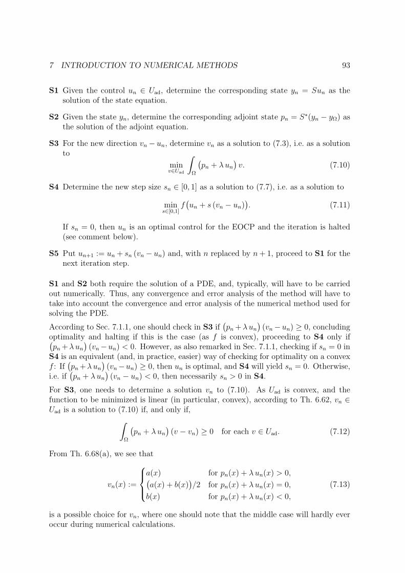
7 INTRODUCTION TO NUMERICAL METHODS 93
S1 Given the control un ∈ Uad, determine the corresponding state yn = Sun as thesolution of the state equation.
S2 Given the state yn, determine the corresponding adjoint state pn = S∗(yn − yΩ) asthe solution of the adjoint equation.
S3 For the new direction vn − un, determine vn as a solution to (7.3), i.e. as a solutionto
minv∈Uad
∫Ω
(pn + λun
)v. (7.10)
S4 Determine the new step size sn ∈ [0, 1] as a solution to (7.7), i.e. as a solution to
mins∈[0,1]
f(un + s (vn − un)
). (7.11)
If sn = 0, then un is an optimal control for the EOCP and the iteration is halted(see comment below).
S5 Put un+1 := un + sn (vn − un) and, with n replaced by n+ 1, proceed to S1 for thenext iteration step.
S1 and S2 both require the solution of a PDE, and, typically, will have to be carriedout numerically. Thus, any convergence and error analysis of the method will have totake into account the convergence and error analysis of the numerical method used forsolving the PDE.
According to Sec. 7.1.1, one should check in S3 if(pn+λun
)(vn−un) ≥ 0, concluding
optimality and halting if this is the case (as f is convex), proceeding to S4 only if(pn+λun
)(vn−un) < 0. However, as also remarked in Sec. 7.1.1, checking if sn = 0 in
S4 is an equivalent (and, in practice, easier) way of checking for optimality on a convexf : If
(pn+λun
)(vn−un) ≥ 0, then un is optimal, and S4 will yield sn = 0. Otherwise,
i.e. if(pn + λun
)(vn − un) < 0, then necessarily sn > 0 in S4.
For S3, one needs to determine a solution vn to (7.10). As Uad is convex, and thefunction to be minimized is linear (in particular, convex), according to Th. 6.62, vn ∈Uad is a solution to (7.10) if, and only if,∫
Ω
(pn + λun
)(v − vn) ≥ 0 for each v ∈ Uad. (7.12)
From Th. 6.68(a), we see that
vn(x) :=
a(x) for pn(x) + λun(x) > 0,(a(x) + b(x)
)/2 for pn(x) + λun(x) = 0,
b(x) for pn(x) + λun(x) < 0,
(7.13)
is a possible choice for vn, where one should note that the middle case will hardly everoccur during numerical calculations.
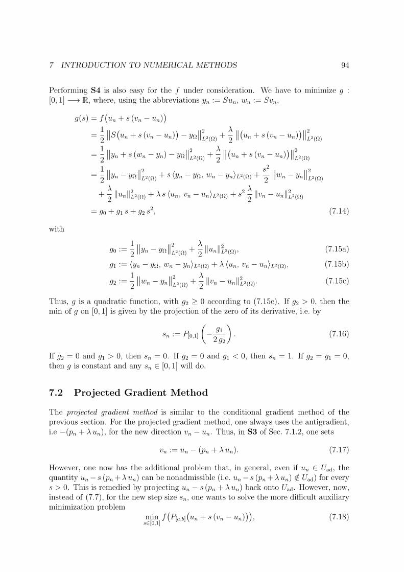
7 INTRODUCTION TO NUMERICAL METHODS 94
Performing S4 is also easy for the f under consideration. We have to minimize g :[0, 1] −→ R, where, using the abbreviations yn := Sun, wn := Svn,
g(s) = f(un + s (vn − un)
)=
1
2
∥∥S(un + s (vn − un))− yΩ
∥∥2L2(Ω)
+λ
2
∥∥(un + s (vn − un))∥∥2
L2(Ω)
=1
2
∥∥yn + s (wn − yn)− yΩ∥∥2L2(Ω)
+λ
2
∥∥(un + s (vn − un))∥∥2
L2(Ω)
=1
2
∥∥yn − yΩ∥∥2L2(Ω)
+ s 〈yn − yΩ, wn − yn〉L2(Ω) +s2
2
∥∥wn − yn∥∥2L2(Ω)
+λ
2‖un‖2L2(Ω) + λ s 〈un, vn − un〉L2(Ω) + s2
λ
2‖vn − un‖2L2(Ω)
= g0 + g1 s+ g2 s2, (7.14)
with
g0 :=1
2
∥∥yn − yΩ∥∥2L2(Ω)
+λ
2‖un‖2L2(Ω), (7.15a)
g1 := 〈yn − yΩ, wn − yn〉L2(Ω) + λ 〈un, vn − un〉L2(Ω), (7.15b)
g2 :=1
2
∥∥wn − yn∥∥2L2(Ω)
+λ
2‖vn − un‖2L2(Ω). (7.15c)
Thus, g is a quadratic function, with g2 ≥ 0 according to (7.15c). If g2 > 0, then themin of g on [0, 1] is given by the projection of the zero of its derivative, i.e. by
sn := P[0,1]
(− g12 g2
). (7.16)
If g2 = 0 and g1 > 0, then sn = 0. If g2 = 0 and g1 < 0, then sn = 1. If g2 = g1 = 0,then g is constant and any sn ∈ [0, 1] will do.
7.2 Projected Gradient Method
The projected gradient method is similar to the conditional gradient method of theprevious section. For the projected gradient method, one always uses the antigradient,i.e −(pn + λun), for the new direction vn − un. Thus, in S3 of Sec. 7.1.2, one sets
vn := un − (pn + λun). (7.17)
However, one now has the additional problem that, in general, even if un ∈ Uad, thequantity un− s (pn+λun) can be nonadmissible (i.e. un− s (pn+λun) /∈ Uad) for everys > 0. This is remedied by projecting un − s (pn + λun) back onto Uad. However, now,instead of (7.7), for the new step size sn, one wants to solve the more difficult auxiliaryminimization problem
mins∈[0,1]
f(P[a,b]
(un + s (vn − un)
)), (7.18)
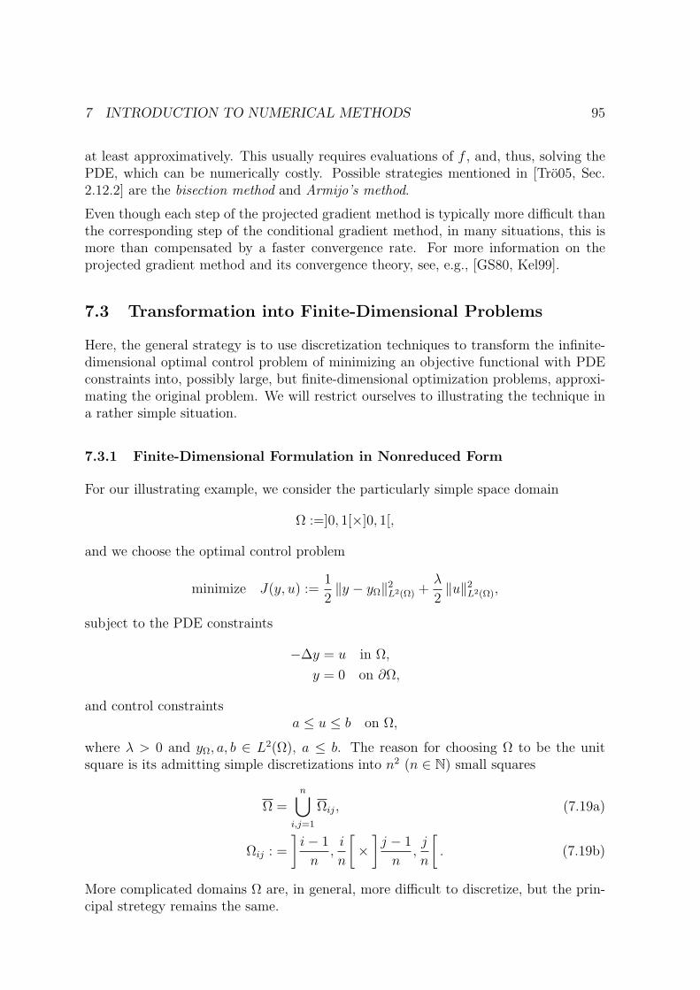
7 INTRODUCTION TO NUMERICAL METHODS 95
at least approximatively. This usually requires evaluations of f , and, thus, solving thePDE, which can be numerically costly. Possible strategies mentioned in [Tro05, Sec.2.12.2] are the bisection method and Armijo’s method.
Even though each step of the projected gradient method is typically more difficult thanthe corresponding step of the conditional gradient method, in many situations, this ismore than compensated by a faster convergence rate. For more information on theprojected gradient method and its convergence theory, see, e.g., [GS80, Kel99].
7.3 Transformation into Finite-Dimensional Problems
Here, the general strategy is to use discretization techniques to transform the infinite-dimensional optimal control problem of minimizing an objective functional with PDEconstraints into, possibly large, but finite-dimensional optimization problems, approxi-mating the original problem. We will restrict ourselves to illustrating the technique ina rather simple situation.
7.3.1 Finite-Dimensional Formulation in Nonreduced Form
For our illustrating example, we consider the particularly simple space domain
Ω :=]0, 1[×]0, 1[,
and we choose the optimal control problem
minimize J(y, u) :=1
2‖y − yΩ‖2L2(Ω) +
λ
2‖u‖2L2(Ω),
subject to the PDE constraints
−∆y = u in Ω,
y = 0 on ∂Ω,
and control constraintsa ≤ u ≤ b on Ω,
where λ > 0 and yΩ, a, b ∈ L2(Ω), a ≤ b. The reason for choosing Ω to be the unitsquare is its admitting simple discretizations into n2 (n ∈ N) small squares
Ω =n⋃
i,j=1
Ωij, (7.19a)
Ωij : =
]i− 1
n,i
n
[×]j − 1
n,j
n
[. (7.19b)
More complicated domains Ω are, in general, more difficult to discretize, but the prin-cipal stretegy remains the same.
7 INTRODUCTION TO NUMERICAL METHODS 96
To proceed further, we introduce the (n+ 1)2 points
xij := (hi, hj), h :=1
n, i, j = 0, . . . , n,
with neighborhoodsΩij := Bh
2,‖·‖max
(xij).
Thus, the xij are precisely the vertices of the squares Ωij as well as the centers of theΩij. The goal is to determine values yij as solutions to a suitable finite-dimensionaloptimization problem such that yij ≈ y(xij), i.e. such that the yij are approximationsto the value of y at xij (or on Ωij).
Using difference quotients of difference quotients, one obtains the classical approxima-tion
−∆y(xij) = −∂1∂1y(xij)− ∂2∂2y(xij) ≈4yij − (yi−1,j + yi,j−1 + yi+1,j + yi,j+1)
h2. (7.20)
At the boundary of Ω, we use
y0j := yi0 := ynj := yin := 0 for each i, j = 0, . . . , n.
Analogous to the yij, we introduce approximations
uij ≈ u(xij), yΩ,ij ≈ yΩ(xij), aij ≈ a(xij), bij ≈ b(xij),
where yΩ,ij, aij, bij have to be computed from the given functions yΩ, a, b, respec-tively, whereas the uij constitute additional unknowns to be determined from the finite-dimensional optimization problem below. By employing an enumeration of the indexset (i, j) : i, j = 1, . . . , n− 1, we organize the yij, uij, yΩ,ij, aij, and bij into vectors
~y = (y1, . . . , y(n−1)2), ~u = (u1, . . . , u(n−1)2), ~yΩ = (yΩ,1, . . . , y(n−1)2),
~a = (a1, . . . , a(n−1)2), ~b = (b1, . . . , b(n−1)2),
respectively. Approximating the functions y, u, and yΩ as being constant on each Ωij
with values according to the above approximations, one obtains
J(y, u) =1
2
∫Ω
(y − yΩ)2 +
λ
2
∫Ω
u2 =1
2
n∑i,j=0
∫Ωij
((y − yΩ)
2 + λu2)
≈ 1
2
n−1∑i,j=1
∫Ωij
((yij − yΩ,ij)
2 + λu2ij
)=
h2
2
n−1∑i,j=1
((yij − yΩ,ij)
2 + λu2ij
).
Thus, our original optimal control problem is translated into the finite-dimensionaloptimization problem
minimize1
2
(n−1)2∑k=1
((yk − yΩ,k)
2 + λu2k
),
7 INTRODUCTION TO NUMERICAL METHODS 97
subject to the equation constraints
Ah ~y> = ~u>,
and control constraints~a ≤ ~u ≤ ~b
for the unknown components of ~y and ~u, where the entries of the matrix Ah are givenaccording to (7.20). Discrete optimization problems of this form can, for example, besolved by the MATLAB function quadprog.
That the size of the discrete problem is typically large, is a drawback of the approachconsidered in the present section. It is often useful to obtain smaller problems bydiscretizing the reduced optimal control problem, which is discussed in the next section.
7.3.2 Finite-Dimensional Formulation in Reduced Form
The strategy of the previous section consists of discretizing the nonreduced optimalcontrol problem directly, i.e. the variable y is not eliminated by writing it as a functionof u. In contrast, in the following, we will employ the PDE’s solution operator S toeliminate the variable y. We start by discretizing u. Here, the idea is to approximateu as a finite linear combination of M basis functions e1, . . . , eM , M ∈ N,
u(x) ≈M∑k=1
uk ek(x), uk ∈ R.
Continueing to employ the notation introduced in the previous section, for the ek, wechoose the M = n2 characteristic functions
1Ωij(x) :=
1 for x ∈ Ωij,
0 for x ∈ Ω \ Ωij.
Next, we introduce the functions
yk := S(ek), k = 1, . . . ,M,
where S : L2(Ω) −→ L2(Ω) is the PDE’s solution operator according to Th. 6.43.
In practice, the computation of the yk means the numerical solution of n2 PDE. Andas a fine discretization of Ω can be necessary to achieve an acceptable accuracy for theapproximation of u, this can be computationally costly. However, in Sec. 7.3.3 below,we will see a trick to avoid the computation of the yk.
Plugging the approximations for u into J(y, u) = J(Su, u) yields the finite-dimensionaloptimization problem
minimize fh(~u) = fh(u1, . . . , uM) :=1
2
∥∥∥∥∥M∑k=1
uk yk − yΩ
∥∥∥∥∥2
L2(Ω)
+λ
2
∥∥∥∥∥M∑k=1
uk ek
∥∥∥∥∥2
L2(Ω)
,
(7.21a)
7 INTRODUCTION TO NUMERICAL METHODS 98
subject to the control constraints~a ≤ ~u ≤ ~b (7.21b)
for the unknown components of ~u. In order to solve (7.21), we rewrite fh(~u) by makinguse of the inner product in L2(Ω):
fh(~u) =1
2‖yΩ‖2L2(Ω) −
⟨yΩ,
M∑k=1
uk yk
⟩+
1
2
⟨M∑k=1
uk yk,M∑l=1
ul yl
⟩
+λ
2
⟨M∑k=1
uk ek,M∑l=1
ul el
⟩
=1
2‖yΩ‖2L2(Ω) −
M∑k=1
uk 〈yΩ, yk〉+1
2
M∑k,l=1
ukul 〈yk, yl〉+λ
2
M∑k=1
ukul 〈ek, el〉.
Since 12‖yΩ‖2L2(Ω) is constant, (7.21) is equivalent to
minimize fh(~u) := ~v ~u> +1
2~uC~u> +
λ
2~uD~u>, (7.22a)
subject to the control constraints~a ≤ ~u ≤ ~b (7.22b)
for the unknown components of ~u, where
~v := (vk)Mk=1, vk := −〈yΩ, yk〉,
C := (ckl)Mk,l=1, ckl := 〈yk, yl〉,
D := (dkl)Mk,l=1, dkl := 〈ek, el〉.
Note that due to the choice of the ek as the characteristic functions of the disjoint setsΩij, the matrix D is diagonal:
〈ek, el〉 =
‖ek‖2L2(Ω) for k = l,
0 for k 6= l.
Once again, (7.22) can, for example, be solved by the MATLAB function quadprog.
7.3.3 Trick to Solve the Reduced Form Without Formulating it First
The numerical solution of the finite-dimensional optimization problem (7.22), requirescomputations of expressions of the form D~x and C~x with x ∈ RM , where for large Mone should only store the nonzero elements of D and C. While expressions of the formD~x are easy to compute, C~x is typically more involved, since C depends on the yk,where yk resulted from solving the PDE with ek on the right-hand side.
7 INTRODUCTION TO NUMERICAL METHODS 99
However, using the following trick, one can evaluate C~x without having to compute theyk first: For each row vector ~x ∈ RM , we have
(C~x)k =M∑l=1
cklxl =M∑l=1
xl 〈yk, yl〉 =M∑l=1
xl 〈Sek, Sel〉 =
⟨S∗S
M∑l=1
xlel, ek
⟩= 〈S∗Sxh, ek〉,
where xh :=∑M
l=1 xlel.
Thus, instead of solving M = n2 PDE once, one now has to solve 2 PDE for every newapplication of C. In general, it will depend on n and on the number of applications ofC needed during the solution of (7.22), which strategy is preferable.
7.4 Active Set Methods
For simplicity, we remain in the setting established in Sec. 7.3.1.
Active set methods are motivated by the observation that, if u is an optimal control,then
u(x) =
a(x) for − p(x)
λ< a(x),
− p(x)λ
for − p(x)λ
∈ [a(x), b(x)],
b(x) for b(x) < − p(x)λ
(7.23)
where p = S∗(Su − yΩ) is the adjoint state (this is due to Ex. 6.69(c), where we havewritten (6.170a) in the equivalent form from (6.164)). The relation (7.23) suggests
that the quantity − p(x)λ
can be considered as a measure for the activity of the controlconstraints.
The continuous version of the active set algorithm reads as follows:
S0 Choose arbitrary initial functions u0, p0 ∈ L2(Ω).
S1 Given the control un and the adjoint state pn, determine the new active sets A+n+1
and A−n+1 as well as the inactive set In+1:
A+n+1 :=
x ∈ Ω : − pn(x)
λ> b(x)
,
A−n+1 :=
x ∈ Ω : − pn(x)
λ< a(x)
,
In+1 := Ω \ (A+n+1 ∪ A−
n+1).
S2 Determine yn+1 and pn+1 from the coupled system of PDE
−∆yn+1 =
a on A−
n+1,
− pn+1
λon In+1,
b on A+n+1,
−∆pn+1 = yn+1 − yΩ.
7 INTRODUCTION TO NUMERICAL METHODS 100
S3 Set
un+1 :=
a on A−
n+1,
− pn+1
λon In+1,
b on A+n+1.
Proceed to S1 for the next iteration step.
Active set methods can be interpreted as Newton methods and, thus, show rapid con-vergence rates [BIK99, KR02].
It remains to formulate the discrete version of the above algorithm. According to thediscretization approach from Sec. 7.3.2, we seek a solution ~u to (7.21). For our presentpurposes, it will be useful to introduce the operator
Sh : RM −→ L2(Ω), Sh(~u) :=M∑k=1
uk yk,
which occurs on the right-hand side of (7.21a) (yk = S(ek) as before). Note that theadjoint operator of Sh is a map S∗
h : L2(Ω) −→ RM .
Steps D2 and D3 of the algorithm below require the computation of expressions of theform S∗
h(Sh~un − yΩ). As we have used ek to denote the basis functions, let εk denotethe standard unit vectors in RM , i.e.
εkl := δkl :=
1 for k = l,
0 for k 6= l.
Then, for u ∈ L2(Ω), the kth component of S∗hu ∈ RM is
(S∗hu)k = 〈S∗
hu, εk〉RM = 〈u, Shεk〉L2(Ω) =
⟨u,
M∑l=1
δkl yl
⟩L2(Ω)
= 〈u, yk〉L2(Ω)
= 〈u, Sek〉L2(Ω) = 〈S∗u, ek〉L2(Ω). (7.24)
Thus, to compute S∗hyΩ, it suffices to solve precisely one PDE, namely the one corre-
sponding to S∗yΩ. Given ~u ∈ RM , by setting u := Sh~u in (7.24), one obtains
(S∗hSh~u)k =
⟨M∑l=1
ulyl, yk
⟩L2(Ω)
=
⟨S∗S
(M∑l=1
ulel
), ek
⟩L2(Ω)
. (7.25)
In consequence, as in Sections 7.3.2 and 7.3.3, one has the choice of either computingthe yk by solving M = n2 PDE once, or solving two PDE whenever an expression of theform S∗
h(Sh~un − yΩ) needs to be calculated. In general, it will depend on the situation(e.g. size of M , desired accuracy, etc.), which strategy is faster.
The discrete active set algorithm can be formulated as follows:
REFERENCES 101
D0 Choose arbitrary initial vectors ~u0, ~p0 ∈ RM .
D1 Given ~un and ~pn, determine the new finite active sets A+n+1 and A−
n+1 as well as thefinite inactive set In+1:
A+n+1 :=
k ∈ 1, . . . ,M : − pn,k
λ> bk
,
A−n+1 :=
k ∈ 1, . . . ,M : − pn,k
λ< ak
,
In+1 := 1, . . . ,M \ (A+n+1 ∪ A−
n+1).
D2 Determine ~un+1 from the linear system
un+1,k =
ak for k ∈ A−
n+1,
−λ−1(S∗h(Sh~un − yΩ)
)k,
bk for k ∈ A+n+1.
D3 Set ~pn+1 := S∗h(Sh~un − yΩ).
Proceed to D1 for the next iteration step.
The iteration is halted once A+n+1 = A+
n and A−n+1 = A−
n . One can show that the activesets must become stationary after finitely many steps and that, at this stage, one canset ~u := ~un to obtain a solution to (7.21) (see [BIK99, KR02]).
References
[Alt06] Hans Wilhelm Alt. Lineare Funktionalanalysis, 5th ed. Springer-Verlag,Berlin, 2006 (German).
[Bet01] J.T. Betts. Practical Methods for Optimal Control Using Nonlinear Program-ming. SIAM, Philadelphia, USA, 2001.
[BIK99] M. Bergounioux, K. Ito, and K. Kunisch. Primal-dual strategy forconstrained optimal control problems. SIAM J. Control and Optimization 37(1999), 1176–1194.
[Els96] J. Elstrodt.Maß- und Integrationstheorie. Grundwissen Mathematik, Sprin-ger-Verlag, Berlin, 1996 (German).
[Eva98] Lawrence C. Evans. Partial Differential Equations. Graduate Studies inMathematics, Vol. 19, American Mathematical Society, Providence, RhodeIsland, 1998, reprinted with corrections in 2002.
[GS80] W.A. Gruver and E.W. Sachs. Algorithmic Methods in Optimal Control.Pitman, London, 1980.
REFERENCES 102
[IT79] A.D. Ioffe and V.M. Tihomirov. Theory of Extremal Problems. Studies inMathematics and its Applications, Vol. 6, North-Holland Publishing Company,Amsterdam, 1979.
[Kel99] C.T. Kelley. Iterative Methods for Optimization. SIAM, Philadelphia, USA,1999.
[KR02] K. Kunisch and A. Rosch. Primal-dual active set strategy for a general classof constrained optimal control problems. SIAM J. on Optimization 13 (2002),321–334.
[KS80] D. Kinderlehrer and G. Stampacchia. An Introduction to VariationalInequalities and their Applications. Pure and Applied Mathematics, Vol. 88,Academic Press, New York, 1980.
[Lio71] J.L. Lions. Optimal Control of Systems Governed by Partial DifferentialEquations, 1st ed. Grundlehren der mathematischen Wissenschaften, Vol. 170,Springer-Verlag, Berlin, 1971.
[Roy88] H.L. Royden. Real Analysis, 3rd ed. Macmillian Publ., New York, 1988.
[RR96] M. Renardy and R.C. Rogers. An Introduction to Partial DifferentialEquations. Texts in Applied Mathematics, Vol. 13, Springer-Verlag, New York,1996, corrected 2nd printing.
[Rud73] W. Rudin. Functional Analyis. McGraw-Hill Book Company, New York, 1973.
[Rud87] W. Rudin. Real and Complex Analysis, 3rd ed. McGraw-Hill Book Company,New York, 1987.
[Tro05] Fredi Troltzsch. Optimale Steuerung partieller Differentialgleichungen.Theorie, Verfahren und Anwendungen, 1st ed. Vieweg Verlag, Wiesbaden, Ger-many, 2005 (German).
[Wer02] D. Werner. Funktionalanalysis, 4th ed. Springer-Verlag, Berlin, 2002 (Ger-man).
[Wlo82] J. Wloka. Partielle Differentialgleichungen. B.G. Teubner, Stuttgart, Ger-many, 1982 (German).
[Yos74] K. Yosida. Functional Analysis, 4th ed. Grundlehren der mathematischenWissenschaften, Vol. 123, Springer-Verlag, Berlin, 1974.
[Zei90] E. Zeidler. Nonlinear Functional Analysis and its Applications. Vol. II/A,Springer-Verlag, New York, 1990.