OPTIMAL CONTROL OF DIABETES MELLITUS UNDER TIME DEPENDENT UNCERTAINTIES

Saadet Ulas Acikgoz, Urmila M. Diwekar, University of Illinois at Chicago, Department of Bioengineering,Chicago, IL, Vishwamitra Research Institute, Westmont, IL

Abstract

Diabetes is a disease resulting from the impaired mechanism of insulin secretion from the pancreas, which prevents glucose from entering the cells and be utilized, which leads to wide swings of blood sugar and many complications such as heart disease and stroke, kidney disease and amputations. In order to prevent these complications and achieve a better quality of life for diabetic patients, effective regulation of blood glucose is essential. This study aims to achieve a better blood glucose control profile by incorporating the time-dependent uncertainties in diabetic patient parameters into formulations of optimal control using a novel approach which originates from finance literature. The time-dependent uncertainties are represented using stochastic processes called Ito processes and the mathematical formulation for this problem is presented. This new method was previously implemented on batch separation problem in an earlier study, where the process yields were significantly improved [Ulas S. and Diwekar, U.M. (2004), Comp. Chem. Eng. 28(11):2245-2258] and it holds a lot of promise in reducing the wide swings of blood glucose observed in diabetic patients and preventing possible complications of diabetes.

Introduction

20.8 million people in the U.S. suffer from diabetes, which has many complications such as heart disease and stroke, high blood pressure, kidney disease, nervous system disease and amputations. The hormone insulin has many functions in the body; most importantly it influences the entry of glucose into cells. The lack of insulin prevents glucose from entering the cells and be utilized, which leads to excess blood sugar and excretion of large volumes of urine, dehydration and thirst. The current treatment methods for insulin-dependent diabetes include subcutaneous insulin injection or continuous infusion of insulin via an insulin pump. The former treatment requires patients to inject insulin four to five times a day. The amount of injection is usually determined by a glucose measurement, an approximation of the glucose content of the upcoming meal and estimated insulin release kinetics. The continuous insulin infusion pump allows for more predictable delivery due to its constant infusion rate into a subcutaneous delivery site. Keeping the blood glucose levels as close to normal (non-diabetic) as possible is essential for preventing diabetes related complications. Ideally this level is between 90 and 130 mg/dl before meals and less than 180 two hours after starting a meal. The Diabetes Control and Complications Trial (DCCT) followed 1441 people with diabetes for several years. This trial concluded that the patients who followed a tight glucose control program were less likely to develop complications such as eye disease, kidney disease and nerve disease, than the ones who followed the standard treatment, because the former group had kept the blood glucose levels lower.

The ideal treatment for controlling blood glucose levels in insulin dependent diabetic patients would be the use of an artificial pancreas which would have the following components: (a) a glucose

sensor which monitors the blood glucose continuously with sufficient reliability and precision; (b) a computer which could calculate the necessary insulin infusion rates by an appropriate feedback algorithm; (c) an insulin infusion pump which would release the required amount of insulin into the blood. However, safe delivery of insulin in this way requires reliable glucose sensors. Two types of sensors have been developed during the last 30 years, minimal invasive and non-invasive (Koschinsky and Heinemann, 2001). The non-invasive approaches are carried out using optical glucose sensors. These sensors work by directing a light beam through intact skin and measuring the properties of the reflected light that are altered either as a result of direct interaction with glucose (spectroscopic approach) or due to the indirect effects of glucose by inducing changes in the physical properties of skin (scattering approach). However, these optical sensors are not able to measure glucose with sufficient precision. On the other hand, minimally invasive sensors measure the glucose concentration in the interstitial fluid of the skin or in the subcutis. There is a free and rapid exchange of glucose molecules and interstitial fluid. Therefore, changes in blood glucose and interstitial glucose are correlated. However, there is a time delay between these changes varying from a few seconds to 15 minutes; which complicates the interpretation of measurement results (Roe and Smoller, 1998). The magnitude of this delay depends on factors such as the absolute glucose concentrations and direction of change. This delay shows intra and inter-individual variability. Furthermore, it has been found that the absolute values of interstitial glucose concentrations vary between 50 and 100% of the intravasal value. The wide-spread use of these glucose sensors is also complicated by biocompatibility issues and skin reactions. Also these sensors should be available at a reasonable cost in order to be applicable to insulin-dependent diabetic patients. The implementation of a closed loop system in daily life conditions requires these reliability, compatibility, cost and safety issues to be resolved.

The aim of this paper is to develop an optimal control system. Optimal control is different from a closed loop feedback control where the desired operating point is compared with an actual operating point and knowledge of the difference is fed back to the system. Optimal control problems are defined in their time domain, and their solution requires establishing an index of performance for the system and designing the course (future) of action so as to optimize a performance index. Therefore optimal control allows us to make future decisions. Using optimal control theory we can minimize the deviations of blood glucose from non-diabetic levels, while penalizing the use of large amounts of infused insulin for safety. Swan (1982), Fisher and Teo (1989), Ollerton (1989), Fisher (1991) and Parker et al. (1999) applied optimal control theory to this problem. However, uncertainties in model parameters and variability among different individuals were not considered in these papers.

The optimal control problem formulation involves finding the set of insulin infusion rates {uk} that minimizes a cost criterion which is the deviations of blood glucose from a preset level over time, where a “minimal model” is used to represent insulin/glucose dynamics, which means that the model uses the smallest number of parameters and yet it satisfies certain validation criteria. This model was developed by Bergman et al. (1985). In this model, insulin is assumed to affect glucose levels via a remote compartment X and physiological parameters become “lumped” together in the resulting equations. The problem formulation is as follows (Fisher, 1991). Find the set of insulin infusion rates u(t) that minimizes the cost criterion:

∫=T

dttGJ0

21 )(

subject to: )()(1 tPGGXGpdtdG

B +−−−= (1)

IpXpdtdX

32 +−= (2)

)()(B

I

IInV

tudtdI

+−= (3)

with maxmin uuu ≤≤ (4)

and 0)0( GG = 0)0( XX = 0)0( II = (5)

The following terms are used in the model: represents plasma glucose level (mmol/l), models insulin effect to facilitate plasma glucose uptake (min

)(tG)(tX -1), is the insulin level above

basal (mU/l), is the basal insulin level (mU/l), is the basal glucose level (mmol/l), are subject-dependent model parameters (min

)(tI

BI BG nppp ,,, 321-1), =p4p 1GB (mmol/l/min), is the exogenous

glucose infusion rate (mmol/l/min), is the insulin infusion rate (mU/l/min), which is the control variable, are the lower and upper insulin infusion rate bounds, for reasons of safety, is the insulin distribution volume and are the initial values of G, X and I respectively.

)(tP)(tu

maxmin ,uu IV

000 ,, IXGAmong the subject-dependent model parameters, p1 describes glucose effectiveness, which is

the net effect of glucose by itself, at basal insulin, to normalize the glucose concentration within the extracellular glucose pool. On the other hand, the ratio between p3 and p2 defines the insulin sensitivity index, which represents the insulin dependent increase in the net glucose disappearance rate. Additionally, n represents the fractional insulin clearance. These subject-dependent model parameters are obtained by a data fitting procedure.

The success of optimal control method depends on the accuracy of the model; therefore, the inherent uncertainties in the patient need to be addressed. If the uncertainties are omitted and if the model cannot accurately represent the glucose and insulin dynamics, this can lead to significant performance degradation. Significant variability of relevant parameters among patients and within a given patient during the course of the day or week has been reported in literature (Simon et al., 1987; Bremer and Gough, 1999). Meals and exercise, the age and weight of the patient also affect the insulin/glucose dynamics. These daily and hourly fluctuations of patient parameters can create difficulties in continuous glucose control. These dynamic uncertainties affect the optimal insulin infusion profiles.

The aim of this paper is to model these uncertainties by a novel approach and incorporating them into formulations of optimal control. Time-dependent uncertainties are commonly encountered in finance literature. Dixit and Pindyck (1994) and Metron and Samuelson (1990) described optimal investment rules developed for pricing options in financial markets, and Ito’s Lemma to generalize the Bellman equation or the fundamental equation of optimality for the stochastic case. This new equation constitutes the base of the so called Real Options Theory. Although such a theory was developed in the field of economics, it was recently applied to optimal control problems encountered in other branches of science. For example, in chemical engineering literature, time-dependent uncertainties in batch processing and pharmaceutical separations were represented by Ito processes and time-dependent stochastic optimal control profiles were obtained. Using this approach, the performance of separation processes where stochastic optimal control was applied, has increased significantly as high as 69%. Using Ito processes, ideal and non-ideal systems were represented and thermodynamic parameter uncertainties associated with locally optimal parameter estimates as a result of nonlinear regression were addressed (Ulas and Diwekar, 2004; Ulas et al., 2005).

This approach could also be extended to optimal glucose control in insulin dependent diabetic patients. The patient parameters can be forecasted from previous data using Ito processes and stochastic optimal control profiles could be derived to achieve better treatment for diabetes. This study aims to explore the possibility of using options theory from finance for dealing with time dependent uncertainties in diabetes optimal control and to develop efficient methods to characterize, quantify and propagate static and time-dependent uncertainties in diabetic patient models and model parameters and to improve the effectiveness of glucose control for insulin-dependent diabetic patients.

Uncertainties in Diabetes Glucose Control

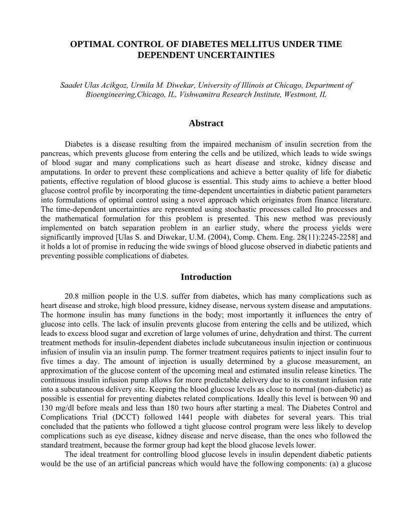
It is well known that there is considerable variability among daily values of glucose and. Due to this variability, even the same insulin dose with the same meal and the same amount of physical exercise may result in different blood glucose responses on consecutive days. Furthermore, blood glucose levels vary among different patients according to meals, exercise levels, age and stress. This natural inter- and intra-patient variability needs to be addressed in developing an optimal glucose control profile. For characterizing, quantifying and propagating static and time-dependent uncertainties in diabetic patient parameters two methods can be used. For static uncertainties this techniques is the stochastic modeling framework. For dynamic uncertainties, stochastic processes called Ito processes can be used. Modeling Static Uncertainties – Stochastic Modeling Framework An example of a static uncertainty is the parameters of the mathematical model used to represent the blood glucose dynamics. The uncertainties in model parameters can be represented using probabilistic techniques and stochastic modeling (Figure 1). Probabilistic or stochastic modeling achieves this using an iterative procedure involving these steps (Diwekar & Rubin, 1991):

1. Specifying uncertainties in model parameters in terms of probability distributions 2. Sampling the distribution of the specified parameter in an iterative fashion 3. Propagating the effects of uncertainties through the model 4. Applying statistical techniques to analyze the results.

Process Simulator

Stochastic Modeler

Analysis of output variables

Figure 1: Stochastic Modeling Framework

Modeling Dynamic Uncertainties – Stochastic Processes Since the interactions between insulin, meals, exercise and other factors and their effect on blood glucose is a dynamic phenomenon, it involves dynamic uncertainties or variations. These dynamic uncertainties (variabilities) could be represented using stochastic processes. A stochastic process is a variable that evolves over time in an uncertain way. One of the simplest examples of a stochastic process is the random walk process. The Wiener process, also known as Brownian motion (Figure 2a shows one form of Brownian motion) is a continuous limit of the random walk and is a continuous time stochastic process. A Wiener process can be used as a building block to model an extremely broad range of variables that vary continuously and stochastically through time. An example of this is the price of technology stock. It fluctuates randomly, but over a long time period has had a positive expected rate of growth that compensates investors for risk in holding the stock. A Wiener process has three important properties: 1. It satisfies the Markov property. The probability distribution for all future values of the process depends only on its current value. Stock prices can be modeled as Markov processes, on the grounds that public information is quickly incorporated in the current price of the stock and past pattern has no forecasting value. 2. It has independent increments. The probability distribution for the change in the process over any time interval is independent of any other time interval (non-overlapping). 3. Changes in the process over any finite interval of time are normally distributed, with a variance that increases linearly with the time interval. From the example of the technology stock above, it is easy to show that the variance of the change distribution can increase linearly, in a manner similar to Brownian motion with drift shown in Figure 2a. However, given that stock prices can never fall below zero, price changes cannot be represented as a normal distribution. To get around this difficulty, it is reasonable to assume that changes in the logarithm of prices are normally distributed. Thus, stock prices can be represented by logarithm of a Wiener process. Stochastic processes do not have time derivatives in the conventional sense and, as a result, they cannot be manipulated using the ordinary rules of calculus as needed to solve stochastic optimal control problems. Ito (1951, 1974) provided a way around this by defining a particular kind of uncertainty representation based on the Wiener process as a building block. An Ito process is a stochastic process, x(t), whose increment, dx, is represented by the equation: dztxbdttxadx ),(),( += (6) where dz is the increment of a Wiener process, and a(x, t) and b(x, t) are known functions. By definition, E(dz) = 0 and (dz)2 = dt where E is the expectation operator and E(dz) is interpreted as the expected value of dz. The simplest generalization of Equation (6) is the equation for Brownian motion with drift given by: dzdtdx σα += Brownian motion with drift (7) where α is called the drift parameter, and σ is the variance parameter. Figure 2a shows the sample paths of Equation (7). Other examples of Ito processes are the geometric Brownian motion with drift (Equation (8) given below) and the mean reverting process (Equation (9) and Figure 2(b)). xdzxdtdx σα += Geometric Brownian motion with drift (8) In geometric Brownian motion, the percentage changes in x and ∆x/x are normally distributed (absolute changes are lognormally distributed). In mean reverting processes, the variable may fluctuate randomly in the short run, but in the longer run it will be drawn back towards the nominal value of the variable:

(b)(a)

Figure 2: Sample paths for: (a) a Brownian motion with drift, (b) a mean reverting process (reproduced from Diwekar, 2003)

dzdtxxdx ση +−= )( Mean reverting process (9) where η is the speed of reversion and x is the nominal level that x reverts to. It was shown in our earlier work related to batch processing in pharmaceutical and biotechnology related industries that thermodynamic uncertainties can be represented by Ito processes. Batch distillation is an important separation process for small-scale production especially in pharmaceutical, specialty chemical and biochemical industries. The stochastic optimal control policy was applied to batch distillation in order to optimize the column operating policy by selecting a trajectory for reflux ratio (control variable). The time-dependent uncertainties in relative volatility, which is a thermodynamic parameter that provides the equilibrium relationship between the vapor and liquid phases, was represented by Ito processes, both for ideal and non-ideal systems (Rico-Ramirez et al., 2003, Ulas, 2003, Ulas and Diwekar, 2004). For non-ideal, azeotropic mixtures, the usefulness of this approach becomes more evident, since the effects of thermodynamic uncertainties are more significant. It was shown that for non-ideal system, the dynamic behavior of relative volatility is best modeled with a geometric mean reverting process. This is illustrated in Figure 3.

0

0.5

1

1.5

2

2.5

3

3.5

4

4.5

5

0 0.5 1 1.5 2time (h)

rela

tive

vola

tility

plate 1

plate 2

plate 3

plate 4

plate 5

plate 6

plate 7

plate 8

plate 9

plate 100

0.5

1

1.5

2

2.5

3

3.5

4

4.5

5

0 0.5 1 1.5time(h)

rela

tive

vola

tility

2

(a) (b)

Figure 3: Relative volatility as an Ito process. (a) the change of relative volatility with respect to time

and plate in a batch distillation column for the ethanol-water system, (b) Sample paths of a geometric mean reverting process with 66% confidence intervals (Ulas and Diwekar, 2004)

As stated earlier, stochastic processes do not have time derivatives in the conventional sense and, as a result, they cannot always be manipulated using the ordinary rules of calculus. This is because, in general the solution to a stochastic differential equation is not a single value for the function, but rather is a probability distribution. To work with stochastic processes, one must make use of Ito’s Lemma. This Lemma, called the Fundamental Theorem of Stochastic Calculus, allows us to differentiate and to integrate functions of stochastic processes. Time dependent profiles (optimal control) can then be derived for these stochastic processes. In order to illustrate the usefulness of this approach, a known system was used, namely, the ethanol-water system presented earlier (Figure 4). For the optimal control problem, the system considered is 100 kmol of ethanol-water being processed in a batch column with 1 atm pressure, 13 theoretical stages, 33 kmol/h vapor rate and the batch time is 2 hours. For this problem, the purity constraint on the distillate is specified as 90%. The optimal reflux and distillate profiles for the stochastic case and the deterministic case are shown in Figure 4. Please note that, there is a significant difference between the two profiles. These two profiles (Figure 4a) for the reflux ratio are given to a rigorous simulator MultiBatchDSTM (Diwekar, 1996) to compare the process performance (Figure 4b) when there are thermodynamic uncertainties. It has been found that the average purity results of rigorous simulation are almost the same at about 90% for both of these cases. However, for the deterministic case the distillate amount is 69 % lower than the stochastic case. This case study shows the importance of including the effect of dynamic uncertainties in optimal control formulation. However, it should be noted that the typical mathematical techniques used to solve optimal control problems (calculus of variations), Pontryagin’s maximum principle, and nonlinear programming algorithms) cannot be directly applied to the problem of optimal control under dynamic uncertainties. As stated earlier, real options theory uses Ito’s Lemma and dynamic programming to solve the problem of stochastic optimal control. However, it has been acknowledged that the equations resulting from stochastic dynamic programming are cumbersome and computationally inefficient to solve. The next sub-section presents a novel approach based on stochastic maximum principle to solve this problem.

0123456789

1011

0 0.5 1 1.5 2 2.5

0

5

10

15

20

0 0.5 1 1.5 2 2.5

TIME (h)

D (K

MO

LES)

stochastic casedeterministic case

time

reflu

x ra

tio stochastic case

deterministic case

Figure 4: Optimal profiles for the ethanol-water system (Ulas and Diwekar, 2004) Optimal Control and Stochastic Maximum Principle

Optimal control problems in engineering have received considerable attention in the literature. In general, solutions to these problems involve finding the time-dependent profiles of the control variables so as to optimize a particular performance index. The dynamic nature of the decision variables makes these problems much more difficult to solve compared to optimization problems

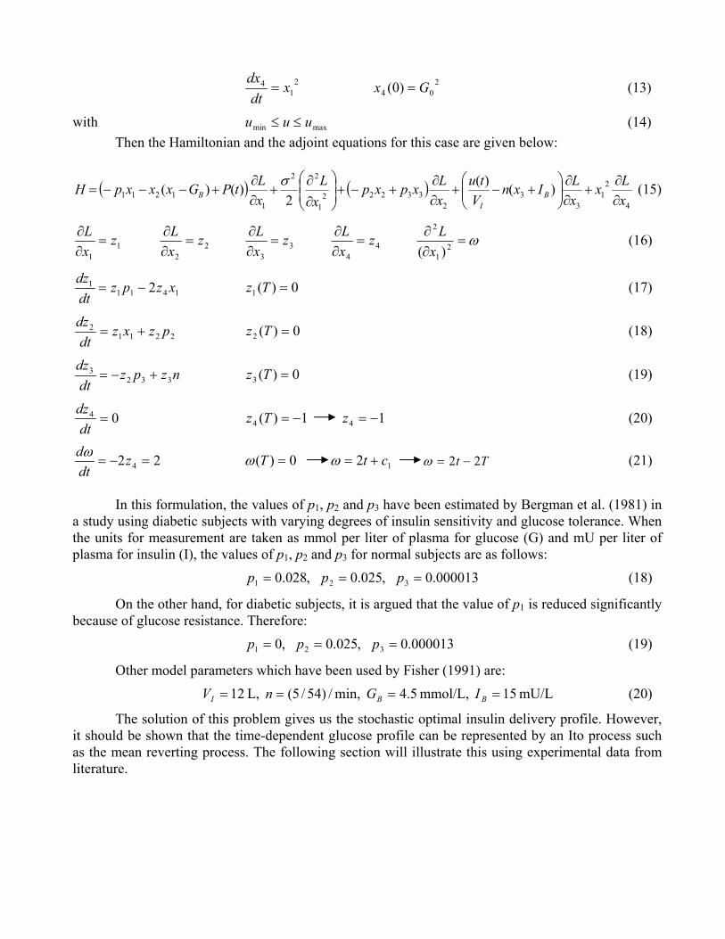
where the decision variables are scalar. In general mathematical methods to solve these problems involve calculus of variations, the maximum principle and the dynamic programming technique. Nonlinear Programming (NLP) techniques can also be used to solve this problem provided all the system of differential equations is converted to nonlinear algebraic equations. For details of these methods please refer to Diwekar(2003). Calculus of variations considers the entire path of the function and optimizes the integral by minimizing the functional by vanishing the first derivative, resulting in second-order differential equations that can be difficult to solve. Other two approaches keep the first order differential system as is but use transformation. In the maximum principle (Boltyanskii et al., 1956; Pontryagin, 1957) the objective function is reformulated as a linear function in terms of final values of state variables and the values of a vector of constants (Mayer Linear form). However, this maximum principle transformation needs to include additional variables and corresponding first order differential equations, referred to as adjoint variables and adjoint equations, respectively. Dynamic programming formulation (Dreyfus, 1965) results in first order system of partial differential equations (the Hamilton-Jacobi-Bellman, HJB equations) that may not be easy to solve. However, this dynamic programming method provides the basis for stochastic optimal control problems and real options theory. Although the mathematics of dynamic programming look different from the maximum principle formulation, in most cases they lead to the same results. This is not surprising and has been reported elsewhere (See for instance Diwekar, 1994; Diwekar, 2003) for the deterministic case. Financial literature reports an extension of the HJB equation for the stochastic case (Dixit and Pindyck, 1994; Thompson and Sethi, 1994; Merton and Samuelson, 1990) but an equivalent maximum principle is not reported. In this study, the mathematical equivalence between dynamic programming and the maximum principle is used to extend the maximum principle to the stochastic case. The main aspect of the derivation involves obtaining the expressions for the adjoint equations. The adjoint equations provide the dynamics of the adjoint variables in the maximum principle. For the deterministic case, it is shown that the adjoint variables in the maximum principle are equivalent to the derivatives of the objective function with respect to the state variables of the dynamic programming approach. Such equivalence is kept for the stochastic case and provides the basis of the reformulation. For more details on this derivation and its application to a batch distillation column (stochastic optimal control policy), please refer to Diwekar (2003), Rico-Ramirez et al. (2003) and Ulas et al. (2004). Let us consider the optimal control problem for blood glucose control presented previously. If we establish that the time-dependent glucose profiles can be represented by an Ito process such as the mean reverting process, the model equations are given below. Let us define a variable x4: Maximize –x4(T)

∫=T

dttxx0

214 )(

subject to: dztPGxxxpdx B σ++−−−= )()( 12111 , 01 )0( Gx = (10)

33222 xpxp

dtdx

+−= , 02 )0( Xx = (11)

)()(3

3B

I

IxnV

tudt

dx+−= , 03 )0( Ix = (12)

21

4 xdt

dx= (13) 2

04 )0( Gx =

with maxmin uuu ≤≤ (14) Then the Hamiltonian and the adjoint equations for this case are given below:

( ) ( )4

21

33

233222

1

22

11211 )()(

2)()(

xLx

xLIxn

Vtu

xLxpxp

xL

xLtPGxxxpH B

IB ∂

∂+

∂∂

⎟⎟⎠

⎞⎜⎜⎝

⎛+−+

∂∂

+−+⎟⎟⎠

⎞⎜⎜⎝

⎛

∂∂

+∂∂

+−−−=σ (15)

11

zxL=

∂∂ 2

2

zxL=

∂∂ 3

3

zxL=

∂∂ 4

4

zxL=

∂∂ ω=

∂∂

21

2

)( xL (16)

14111 2 xzpz

dtdz

−= (17) 0)(1 =Tz

22112 pzxz

dtdz

+= (18) 0)(2 =Tz

nzpzdt

dz332

3 +−= (19) 0)(3 =Tz

04 =dt

dz 1)(4 −=Tz 14 −=z (20)

22 4 =−= zdtdω 0)( =Tω 12 ct +=ω Tt 22 −=ω (21)

In this formulation, the values of p1, p2 and p3 have been estimated by Bergman et al. (1981) in a study using diabetic subjects with varying degrees of insulin sensitivity and glucose tolerance. When the units for measurement are taken as mmol per liter of plasma for glucose (G) and mU per liter of plasma for insulin (I), the values of p1, p2 and p3 for normal subjects are as follows: 000013.0 ,025.0 ,028.0 321 === ppp (18)

On the other hand, for diabetic subjects, it is argued that the value of p1 is reduced significantly because of glucose resistance. Therefore: 000013.0 ,025.0 ,0 321 === ppp (19)

Other model parameters which have been used by Fisher (1991) are: mU/L 15 mmol/L, 4.5 min,/)54/5( L, 12 ==== BBI IGnV (20)

The solution of this problem gives us the stochastic optimal insulin delivery profile. However, it should be shown that the time-dependent glucose profile can be represented by an Ito process such as the mean reverting process. The following section will illustrate this using experimental data from literature.

Preliminary Results Experimental Data from Literature One of the important factors that were considered when the experimental data was being collected was the total monitoring period for insulin and glucose. Since this study aims to develop stochastic optimal control profiles for the course of a day, experimental data for glucose or insulin over a 24 hour or a 48 hour period were searched. Also the experimental data had to be taken at short intervals (e.g. minutes) and they should be direct blood or plasma glucose measurements. Similar type of experimental data search was performed by Bremer and co-workers (2001) for glucose sensor development and presented in the website (http://glucosecontrol.ucsd.edu/) One of the examples of this type of data is given in Figure 5. This data is collected from a normal individual who is under continuous enteral nutrition and the glucose and insulin measurements are taken every 10 minutes (Simon et al. 1987). Periodic oscillations in both glucose and insulin profiles are observed in this subject. Another example is given in Figure 6. This data is collected from four different patients over a 48 hour period (Service et al. 1970). The patients are classified according to diabetic stability. An unstable diabetic patient usually shows: (a) wide swings of blood glucose, (b) high and variable diurnal mean blood glucose and urinary glucose and (c) frequent hypoglycemic episodes. These four patients are eating typical meals and receiving single or multiple insulin injections according to the severity of their conditions. Again the experimental data is collected in short intervals over a 48 hour period. In Figure 7, the sample paths of a simple mean reverting process is shown as compared to the experimental data from a stable diabetic patient. The parameters of the simple mean reverting process (Equation 9) were found as 005.0=η , 6.102=x , and 858.2=σ after a data fitting procedure. Among these parameters, x represents the value that x tends to revert to (nominal value), σ represents the standard deviation and η is the speed of reversion. Therefore, for this subject the nominal value of blood glucose was 102.6 mg/100 mL, which is physically meaningful. Figure 8, shows similar results for an unstable diabetic patient, where the parameters of the simple mean reverting process were estimated as 00001.0=η , 0.145=x and 0.9=σ . The small values of η estimated for both subjects show that the systems are slow to return to the nominal values blood glucose x , after a rise or a fall, which is also physically meaningful in a diabetic patient. Furthermore, the nominal value of blood glucose and the standard deviation for the unstable diabetic was estimated to be much higher than the stable diabetic patient. These results are in consent with the fact that unstable diabetics show wide swings of blood glucose and higher values of mean blood glucose.

NORMAL PATIENT

0

50

100

150

200

0 500 1000 1500

time (minutes)

Glu

cose

(mg/

100m

l)

NORMAL PATIENT

0

10

20

30

40

50

60

0 200 400 600 800 1000 1200 1400

time (minutes)

Insu

lin

Figure 5: 24 hour glucose profile and insulin profile for a normal patient receiving continuous enteral nutrition (Simon et al. 1987)

Figure 6: 48 hour glucose profiles for 4 diabetic patients: 2 stable diabetics, 1 moderately unstable diabetic and 1 highly unstable diabetic eating typical meals and receiving single/multiple daily

injections of insulin (Service et al. 1970)

UNSTABLE DIABETIC II

0

50

100

150

200

250

300

0 500 1000 1500 2000 2500 3000

time (minutes)

Blo

od g

luco

se (m

g/10

0mL)

moderately unstable

UNSTABLE DIABETIC I

0

50

100

150

200

250

300

0 500 1000 1500 2000 2500 3000

time (minutes)

Blo

od g

luco

se (m

g/10

0mL)

highly unstable

STABLE DIABETIC II

0

50

100

150

200

0 400 800 1200 1600 2000 2400 2800

time (minutes)

Blo

od g

luco

se (m

g/10

0mL)

STABLE DIABETIC I

0

50

100

150

200

0 400 800 1200 1600 2000 2400 2800

time (minutes)

Blo

od g

luco

se (m

g/10

0mL)

STABLE DIABETIC

050

100150

200250l)

Figure 7: Time dependent glucose profiles for a stable diabetic patient over the course of two days and sample paths of a simple mean reverting process with 005.0=η , 6.102=x and 858.2=σ

0 500 1000time (minutes)

Glu

cose

(mg/

100

m

day 1 day 2 sample path 1sample path 2 sample path 3 sample path 4

UNSTABLE DIABETIC

-200-100

0100200300400500

0 500 1000 1500time (minutes)

Glu

cose

(mg/

100

ml)

day 1 day 2 sample path 1sample path 2 sample path 3

Figure 8: Time dependent glucose profiles for an unstable diabetic patient over the course of two days and sample paths of a simple mean reverting process with 00001.0=η , 0.145=x and 0.9=σ

Summary & Future Work

This study intends to model uncertainties in a biological process such as the regulation of glucose levels inside the body. The patient parameters fluctuate significantly on a daily basis and meal/exercise levels, stress and age affect these fluctuations. These uncertainties prevent conventional deterministic optimal control strategies to be applied to glucose control in insulin dependent diabetic patients. However, it was shown that maintaining blood glucose levels as close to normal (non-diabetic) as possible is essential for preventing diabetes related complications such as heart disease, high blood pressure and stroke, kidney disease and eye disease.

This study aims to explore a novel stochastic optimal control strategy where time-dependent uncertainties in this biological process are represented by Ito processes which originate from finance literature. Using this technique, some of the patient parameters could be forecasted based on earlier data and a stochastic optimal control policy could be derived. This is expected to improve the current treatment methods and provide a better control profile for glucose and prevent complications. References 1. Bergman R., Finegood D., and Ader M. (1985), ‘Assessment of insulin sensitivity in vivo’,

Endocrine Reviews 6: 45-86.

2. Bergman R.N., Lawrence S.P., and Cobelli C., ‘Physiologic Evaluation of Factors Controlling Glucose Tolerance in Man: Measurement of Insulin Sensitivity and β-Cell Glucose Sensitivity From the Response to Intravenous Glucose’, J. Clin. Invest. 68: 1456-1467 (1981).

3. Boltyanskii, V. G., Gamkrelidze, R. V. and Pontryagin, L. S. (1956) ‘On the Theory of Optimum Processes’ (in Russian), Doklady Akad. Nauk SSSR, 110 (1).

4. Bremer T. and Gough D.A. (1999), ‘Is blood glucose predictable from previous values? A solicitation for data’, Diabetes 48: 445-451.

5. Bremer T.M., Edelman S.V., Gough D.A. (2001), ‘Benchmark Data from the Literature for Evaluation of New Glucose Sensing Technologies’, Diabetes Technology and Therapeutics 3 (3): 409-418.

6. Diwekar, U. M. (2003) Introduction to Applied Optimization, Kluwer Academic Publishers, Boston, MA.

7. Diwekar, U. M., (1994) Batch Distillation. Simulation, Optimal Design and Control, Taylor and Francis, Washington, DC, USA.

8. Diwekar, U. M., (1996) ‘Understanding batch distillation process principles with MultiBatchDS’, Computer Applications in Chemical Engineering Education, 4, 275.

9. Dixit A.K. and Pindyck R.S. (1994), Investment under Uncertainty, Princeton University Press, Princeton, NJ.

10. Dixit, A. K. and Pindyck, R.S. (1994) Investment under Uncertainty, Princeton University Press, Princeton, NJ, USA.

11. Dreyfus S. (1965) Dynamic Programming and the Calculus of Variations, Academic Press, New York, NY

12. Fisher M.E. (1991) , ‘A Semi-Closed Loop Algorithm for the Control of Blood Glucose Levels in Diabetics’, IEEE Transactions on Biomedical Engineering 38: 57-61.

13. Fisher M.E. and Teo K.L. (1989), ‘Optimal insulin infusion resulting from a mathematical model of blood glucose dynamics’, IEEE Transactions in Biomedical Engineering 36:479-486.

14. Ito K. (1951) ‘On stochastic differential equations’, Memoirs of American Mathematical Society 4(1).

15. Ito K. (1974) ‘On stochastic differentials’, Applied Mathematics and Optimization, 4, 374 16. Merton R.C., and Samuelson P.A. (1990), Continuous-time Finance, Blackwell Publishing,

Cambridge MA

17. Ollerton R.L. (1989), ‘Application of optimal control theory to diabetes mellitus’. International Journal of Control 50: 2503-2522.

18. Parker R.S., Doyle III F.J. and Peppas N.A. (1999), ‘A model-based algorithm for blood-glucose control in type I diabetic patients’, IEEE Transactions in Biomedical Engineering 46(2): 148-157

19. Potryagin, L. S. (1957) ‘Basic Problems of Automatic Regulation and Control’ (in Russian) Izd-vo Akad Nauk, SSSR.

20. Simon G., Brandenberger G., and Follenius M. (1987), ‘Ultradian oscillations of plasma glucose, insulin and c-peptide in man during continuous enteral nutrition’, Journal of Clinical Endocrinology & Metabolism 64: 669-674.

21. Swan G.W. (1982), ‘An optimal control model of diabetes mellitus’, Bulletin of Mathematical Biology 44: 793-808.

22. Thompson, G. L. and Sethi, S. P. (1994) Optimal Control Theory, Martinus Nijhoff Publishing, Boston, USA.

23. Ulas S. and Diwekar U.M. (2004), ‘Thermodynamic uncertainties in batch processing and optimal control’, Computers and Chemical Engineering 28(11): 2245-2258.

24. Ulas S., Diwekar U.M., and Stadtherr M.A. (2005), ‘Uncertainties in parameter estimation and optimal control in batch distillation’, Computers and Chemical Engineering 29(8): 1805-1814.

©2006