Optimal Control of Constrained Self-Adjoint Nonlinear ...€¦ · J Optim Theory Appl (2016)...

J Optim Theory Appl (2016) 169:735–758DOI 10.1007/s10957-015-0799-4

Optimal Control of Constrained Self-Adjoint NonlinearOperator Equations in Hilbert Spaces

M. A. El-Gebeily1 · B. S. Mordukhovich2 ·M. M. Alshahrani1

Received: 2 February 2015 / Accepted: 17 August 2015 / Published online: 27 August 2015© Springer Science+Business Media New York 2015

Abstract This paper deals with the study of a new class of optimal control prob-lems governed by nonlinear self-adjoint operator equations in Hilbert spaces undergeneral constraints of the equality and inequality types on state variables. While theunconstrained version of such problems has been considered in our preceding publica-tion, the presence of constraints significantly complicates the derivation of necessaryoptimality conditions. Developing a geometric approach based on multineedle con-trol variations and finite-dimensional subspace extensions of unbounded self-adjointoperators, we establish necessary optimality conditions for the constrained controlproblems under considerations in an appropriate form of the Pontryagin MaximumPrinciple.

Keywords Optimal control · Constrained self-adjoint nonlinear operator equationsin Hilbert spaces · Necessary optimality conditions · Maximum principle

Mathematics Subject Classification 49K20 · 47H15 · 93C30

B. S. Mordukhovich: Research of this author was partly supported by the USA National ScienceFoundation under Grants DMS-1007132 and DMS-1512846 and by the USA Air Force Office ofScientific Research under Grant No.15RT0462.

B B. S. [email protected]

M. A. [email protected]

M. M. [email protected]

1 Department of Mathematics and Statistics, King Fahd University of Petroleum and Minerals,Dhahran 31261, Saudi Arabia

2 Department of Mathematics, Wayne State University, Detroit, MI 48202, USA

123

http://crossmark.crossref.org/dialog/?doi=10.1007/s10957-015-0799-4&domain=pdf

736 J Optim Theory Appl (2016) 169:735–758

1 Introduction

The paper concerns optimal control theory to which Professor Elijah (Lucien) Polakhas made fundamental contributions; see, e.g., his seminal book [1]. We consider ageneral class of control systems governed by self-adjoint nonlinear operator equationsin Hilbert spaces formulated and discussed in Sect. 2. Self-adjoint operators coverordinary differential operators, partial differential operators, integral operators, andpseudodifferential operators among others; see, e.g., the books [1–10] and the refer-ences therein. However, to the best of our knowledge, the control model for generaloperator equations, which we first addressed in [11] in the unconstrained setting, hasnever been studied earlier in the literature. Its unconstrained version for singular ODEswas considered in our previous paper [12].

The major result of [11] establishes necessary optimality conditions for optimalcontrols of unconstrained self-adjoint operator equations in Hilbert spaces given inthe form of the Maximum Principle, which is an appropriate operator counterpart ofthe classical Pontryagin Maximum principle for ordinary differential equations [2].The main goal of the current paper is to extend this result to control problems withconstraints on state variables described finitely by many equalities and inequalitiesgiven by Fréchet differentiable functions.

It has beenwell realized in optimal control theory for any type of state equations thatthe presence of even simple constraints on state variables dramatically complicatesthe device of necessary optimality conditions for optimal controls. As shown, e.g.,in [10, Section 6.3], the derivation of the Pontryagin Maximum Principle for ODEsystems without any constraints on system trajectories/arcs can be done by using apure analytic technique via the increment formula for the cost functional on single-needle variations of optimal controls. On the other hand, the presence of smoothendpoint constraints on trajectories required in [10] a much more involved geometrictechnique based on multineedle control variations with the usage of convex separationand delicate fixed-point theorems.

This paper reveals a similar situation in the case of general optimal control prob-lems for nonlinear self-adjoint operator equations with constraints on state variables.We show that developing a geometric technique based on multineedle control varia-tions together with convex separation and fixed-point results allows us to derive anappropriate version of the Maximum Principle for the general constrained operatorcontrol systems under consideration. It should be mentioned to this end that the newlevel of generality encompassed in this paper does not allow us to cover all the specificfeatures of the Maximum Principle for particular types of state equations; see morediscussions in the text below.

The rest of the paper is organized as follows. In Sect. 2 we introduce the class ofconstrained operator control problems of our study and then formulate and discuss thestanding assumptions made on their initial data throughout the whole paper. Section 3recalls some results from [11] onfinite-dimensional subspace extensions of self-adjointoperators, which play a significant role in the subsequent considerations. Based onthese results and given an arbitrary Fréchet differentiable function σ : H → R on thestate space, we construct in Sect. 4 the so-called σ -auxiliary and σ -adjoint problemsto the one under consideration and derive an important formula for representing the

123

J Optim Theory Appl (2016) 169:735–758 737

increment of this function with respect to control variations along the original andadjoint systems.

Section 5 contains the formulation and discussion of our main result–the Maxi-mum Principle for the optimal control problem governed by the general self-adjointoperator equations with constraints on state variables. We also define here the classof multineedle control variations and establish some of their properties needed in thesubsequent proof of the main theorem. The proof in the case of inequality constraintsis given in Sect. 6, while Sect. 7 presents a more involved proof in the case of equal-ity constraints. The final Sect. 8 collects concluding remarks and formulates someproblems of the future research.

Throughout the paper we use the standard notation from theory of operator equa-tions and theory of optimal control; see, e.g., [3,8,10].

2 Problem Formulation and Basic Assumptions

The paper addresses the following optimal control problem: minimize the functional

J [u, x] := ϕ0 (x) subject to u ∈ U , (1)

where admissible control actions u are selected from the given control setU of ametricspace, and where the corresponding states x = xu ∈ H solve the nonlinear operatorequation

˜T x = F (x, u) (2)

and satisfy the constraints of the inequality and equality types:

ϕi (x) ≤ 0 for i = 1, . . . , m, (3)

ϕi (x) = 0 for i = m + 1, . . . , m + r. (4)

Here ˜T : H → H is a given unbounded densely defined self-adjoint operator on theHilbert space H considered over the field of complex numberswith the domain ˜D ⊂ H(the tilde notation will be removed later on for the corresponding extensions of ˜T and˜D needed inwhat follows); F : H ×U → H is a given nonlinear operator on the right-hand side of the operator equation (2); and ϕi : H → R for i = 0, 1 . . . , m + r are thecost and constraint real-valued functions in (1) and (3), (4), respectively. The class ofproblems considered here does not include general first-order initial value problemssince the differential operator involved in this case is not always self-adjoint.

ByAwedenote the set of pairs (u, x) satisfying the operator equation (2)withu ∈ Uand x ∈ ˜D. The symbol B stands for the collection of pairs (u, x) ∈ A such that xsatisfies all the constraints in (3) and (4), which is the set of feasible solutions to thecontrol problem under consideration. Since this paper focuses on deriving necessaryoptimality conditions, we assume that there is a pair (u, x) ∈ B minimizing thecost functional (1) over all (u, x) ∈ B and fix such an optimal pair (u, x) in furtherdiscussions. Throughout the paper we impose the following assumptions on the initialdata in (1)–(4):

123


(H1) The self-adjoint operator ˜T : H → H is bounded below, i.e., there is μ > 0such that

⟨

˜T x, x⟩ ≥ μ ‖x‖2 for all x ∈ ˜D. (5)

(H2) The mapping F : H × U → H is continuous in u and continuously Fréchetdifferentiable in x around x with the partial derivative operator F ′

x (x, u) forany u ∈ U , while the mapping F (·, u) : H → H is weakly continuous andquasimonotone in the following sense: there is ρ < μ, with μ taken from (5),such that

⟨

F (x, u) − F (x, u) , (x − x)⟩ ≤ ρ ‖x − x‖2 for all x ∈ H. (6)

(H3) The cost functional ϕ0 and those for the inequality constraint ϕ1, . . . , ϕm areFréchet differentiable at the optimal point x .

(H4) The equality constraint functionals ϕm+1, . . . , ϕm+r are continuous around xand Fréchet differentiable at this point.

Let us comment on the assumptions above. Note that condition (5) in (H1) impliesthat the spectrum of ˜T is contained in the interval [μ,∞[. Consequently, any λ ∈] − ∞, μ[ is a resolvent point of ˜T meaning that (˜T − λI )−1 is a bounded operatordefined on all of H . In particular, this is true when λ = 0. The assumption that μ > 0can be relaxed to μ ∈ R. The latter situation can be reduced to the former one byreplacing (2) with the equation

(

˜T + δ I)

x = F(x, u) + δx,

where δ > 0 is chosen so that δ + μ > 0, without affecting the results of this paper.Regarding (H2), observe that ρ in (6) does not need to be positive. The only pur-

pose for assuming that F is weakly continuous with respect to x is to ensure theexistence of a solution to (2). It is not used otherwise for the rest of this paper. Otherassumptions that ensure the existence of a solution are also possible. For instance, wecan suppose that either F is completely continuous in x , or that F is continuous in x ,bounded on bounded sets and˜T has the compact resolvent. There is a trade-off betweenrequirements on ˜T and those on F . A general class of such operators satisfying ourassumptions arises from nonlinear functionals in coefficients of basis expansions. Toillustrate it, let gn : C → C, 1 ≤ n ≤ N , be C1 functions with bounded derivatives,{ζn}N

n=1 and {ψn}Nn=1 be two sequences in H . Define the operator G : H → H by

G(x) :=N∑

n=1

gn (〈x, ζn〉) ψn

and consider the operator F : H × U → H given by

F (x, u) := G (x) + h(u),

123


whereh : U → H is continuous inu. Then F (x, u) satisfies all the stated assumptions;see below for more details. This class of nonlinear operators includes some filteringoperators, which are broadly used in, e.g., signal processing.

Observe that, in contrast to the smoothness (C1) requirement on the operator Fwith respect to the state variable x in (H2), the at-point differentiability assumptionson ϕ0, . . . , ϕm+r in (H3) and (H4) are weaker than smoothness (typically requiredin control theory outside of nonsmooth analysis) even in finite dimensions. Thus theoptimal control problem (1)–(4) is not generally smooth with respect to the states x .However, themajor source of nonsmoothness in this infinite-dimensional optimizationproblemcomes from thegeometric constraint on control actionsu ∈ U ; see alsoSect. 5.

To conclude this section, we illustrate the validity of the major assumptions (H1)and (H2) for an interesting class of controlled operator equations (2) in Hilbert spaces.

Example 2.1 (Illustrating major assumptions) Consider the differential equation

−x ′′ (t) + α2x (t) = g(〈x, ζ 〉)ψ + u, x(0) = x(1) = 0,

where α > 0, ζ, ψ ∈ L2 (0, 1) and where g : C → C has bounded derivative; say,∣

∣g′∣∣ ≤ β. Then the operator ˜T x := −x ′′ + α2x on L2 (0, 1) with

˜D ={

x ∈ L2 (0, 1)∣

∣ x, x ′ are absolutely continuous, x ′′ ∈ L2 (0, 1) , x(0)= x(1)=0}

is self-adjoint. Also⟨

˜T x, x⟩ = ∥∥x ′∥

∥

2 + α2 ‖x‖2 ≥ α2 ‖x‖2, and so ˜T satisfies (H1).Denote next F(x, u) := g(〈x, ζ 〉)ψ + u and verify the following properties of this

mapping:• F is Fréchet differentiable and weakly continuous in x . To see this, observe

that ∂∂x g(〈x, ζ 〉)h = g′(〈x, ζ 〉) 〈h, ζ 〉, and hence F ′

x (x, u)h = g′(〈x, ζ 〉) 〈h, ζ 〉 ψ .Assuming now that xn ⇀ x (weakly converges) gives us 〈xn, ζ 〉 −→ 〈x, ζ 〉, and thecontinuity of g ensures that g(〈xn, ζ 〉) −→ g(〈x, ζ 〉). Thus for any v ∈ H we get that

〈g(〈xn, ζ 〉)ψ, v〉 = g(〈xn, ζ 〉) 〈ψ, v〉 −→ g(〈x, ζ 〉) 〈ψ, v〉 = 〈g(〈x, ζ 〉)ψ, v〉 ,

which implies the claimed weak continuity of the mapping F .• F is monotone. Indeed, for any x, y ∈ H we have

〈F(x, u) − F(y, u), x − y〉 = 〈(g(〈x, ζ 〉) − g(〈y, ζ 〉)) ψ, x − y〉≤ ‖(g(〈x, ζ 〉) − g(〈y, ζ 〉)) ψ‖ ‖x − y‖= |g(〈x, ζ 〉) − g(〈y, ζ 〉)| ‖ψ‖ ‖x − y‖≤ β |〈x − y, ζ 〉| ‖ψ‖ ‖x − y‖≤ β ‖ζ‖ ‖ψ‖ ‖x − y‖2 .

Then (H2) is satisfied if β < α2. Note also that introducing

(t, τ ) := 1

α cosh α

{

sinh α(1 − t) sinh ατ, 0 ≤ τ ≤ tsinh α(1 − τ) sinh αt, t ≤ τ ≤ 1

,

123


we can rewrite our system as the integral equation

x (t) = ˜T −1F (x, u) (t) =∫ 1

0 (t, τ ) F (x, u) (τ ) dτ

with the Hilbert–Schmidt kernel (t, τ ) and thus conclude by basic functional analy-sis that the operator ˜T −1 is compact.

While deriving the main result on necessary optimality conditions in Sects. 5–7,we further specify the state and control spaces, imposing in this way an additionalassumption on behavior of the underlying nonlinear operator F in (2) with respect to“needle” variations of the optimal control; see Sect. 5 for more details.

3 Extensions of Self-Adjoint Operators

In this section we recall some notation and results from [11] needed in what follows.Given natural numbers k, r ∈ N and elements X ∈ Hk , Y ∈ Hr from the power

spaces of H , thematrix/operator inner product 〈X, Y 〉 is defined by applying the innerproduct in H to the entries of the formal matrix XY ∗, where the symbol ∗ signifiesthe duality/transposition operation in building the adjoints. In other words,

〈X, Y 〉i j := ⟨xi , y j⟩

as i = 1, . . . , k and j = 1, . . . , r.

It is easy to see that 〈AX, BY 〉 = A 〈X, Y 〉 B∗ whenever A ∈ Cm×k and B ∈ C

d×r ,where C stands as usual for the collection of complex numbers.

Fixing n ∈ N, we say that the components of the vector Z = (z1, . . . , zn) ∈ Hn

are linearly independent modulo ˜D if the inclusion α ∈ C1×n with αZ ∈ ˜D holds

only when α = 0. Let us mention that the assumption that ˜T is self-adjoint impliesthat it is closed. This together with the unboundedness of ˜T mean, by the classicalclosed graph theorem, that ˜D is a proper subspace of H . We should note here that theconstruction described below does not apply to the case of bounded operators, sincein this case the bilinear form defined in (8) is exactly zero. The bounded operator caseis of our ongoing research.

Taking now any number λ ∈ C with Imλ = 0 and the complex conjugate λ, definethe Cayley transform of the operator ˜T by

V := (˜T − λI) (

˜T − λI)−1

,

where I : H → H is the identity operator on H . Denoting further the span of Z =(z1, . . . , zn) by [Z ] := span(Z) and taking its orthogonal complement [Z ]⊥, we formthe new domain

D0 := (I − V ) [Z ]⊥

123


and have the domain representation established in [11]:

˜D = D0 � [W ] with W := (I − V ) Z . (7)

Now we are ready to construct the n-dimensional extension T of the original operator˜T in (2) in the following two-step way:

T0 := ˜T∣

∣

D0and T := T ∗

0 .

It is easy to see that T0 and T are closed operators, T0 is symmetric and relates to ˜Tas

T0 ⊂ ˜T ⊂ T .

Furthermore, the domain D of the extension T relates to the original one ˜D as

D = ˜D � [Z ] .

The operator T generates the antisymmetric sesquilinear form [·, ·] : D × D → C

defined by

[x, y] := 〈T x, y〉 − 〈x, T y〉 , (8)

which can be extended to the product vectors X = (x1, . . . , xk) ∈ Hk and Y =(y1, . . . , yr ) ∈ Hr in the same way as the vector inner products above. We have therelationships

D0 = {x ∈ D∣

∣ [x, W ] = [x, Z ] = 0}

and ˜D = {x ∈ D∣

∣ [x, W ] = 0}

(9)

for the product vectors W and Z under consideration. Moreover, the complex matrices[W, Z ] and [Z , Z ] are isomorphisms in C

n allowing us to show that the equation[W, p] = α is solvable for any given α ∈ C

n ; see [11] for more details.

4 σ -Adjoint Problem and Increment Formula

Having in hands the results of Sect. 3, we can now proceed with constructing theauxiliary and adjoint operator systems to the original one (2) with taking into accountthe cost and constraint functions ϕi , i = 0, . . . , m + r , in the control problem (1)–(4)formulated in Sect. 2. In fact, in this section we are going to do it with respect to anarbitrary differentiable function σ on H , which will be specified later on (Sect. 5) viathe initial data of the control problem under consideration.

Observe first that the self-adjoint property of the operator ˜T in (2) and the imposedboundedness from below assumption (5) in (H1) imply that λ = 0 is a resolvent point

123


for ˜T . Moreover, it follows from the results of Sect. 3 and from [3] that the point λ = 0is of regular type for T0, and we have the equalities

dimR⊥T0 = dim

(

ker T) = n,

where the symbol RT0 stands for the range of the operator T0.Let further the vectors z1, . . . , zn form a basis of the kernel subspace ker T ⊂ H ,

and letwi := ˜T −1zi ∈ ˜D for i = 1, . . . , n. It is easy to see that the relationships in (9)hold with Z := (z1, . . . , zn) and W := (w1, . . . , wn). Denoting by P the projectoroperator onto the closed subspaceRT0 , we get that the mapping (I − P) projects ontothe orthogonal complement of RT0 , which is precisely ker T = [Z ].

For anyw ∈ H and α ∈ Cn consider now the following problems under assumption

(H2):

T y = F ′∗x (x, u) y, [W, y] = α, (10)

˜T y = F ′∗x (x, u) y + w. (11)

It is shown in [11] (see Sect. 3) that under the assumptions made problem (10) admitsthe unique solution p ∈ D, while the uniqueness of the solution q ∈ ˜T to (11) followsfrom the coercivity of the operator ˜T − F ′∗

x (x, u), which is a consequence of theinequality ρ < μ; see assumptions (H1) and (H2).

Next we fix a pair (u, x) ∈ A [which is treated later as an optimal solution to thecontrol problem (1)–(4)] and take an arbitrary function σ : H → R, which is Fréchetdifferentiable at x . Using the function σ and the data of the initial operator equation(2) at (u, x), let us introduce the σ -auxiliary equation

˜T y = F ′∗x (x, u) y − F ′∗

x (x, u) P˜T −1σ ′ (x) , (12)

and the σ -adjoint problem at (u, x) defined via the operator extension T by

T y = F ′∗x (x, u) y, [y, W ] = ⟨σ ′ (x) , W

⟩

. (13)

Observe that the σ -auxiliary equation (12) is the same as (11) with w :=−F ′∗

x (x, u) P˜T −1σ ′ (x) having hence the unique solution q ∈ ˜D, while the σ -adjointproblem (13) is the same as (10) with α := 〈σ ′(x), W 〉 and has therefore the uniquesolution p ∈ D.

The following proposition shows how to obtain a solution to the unified problemconstructed upon (12) and (13).

Proposition 4.1 (Unified solution to the σ -auxiliary and σ -adjoint problems) Letq ∈ ˜D and p ∈ D solve the σ -auxiliary equation (12) and the σ -adjoint problem(13), respectively. Then p := p + q solves the unified problem

T y + F ′∗x (x, u) P˜T −1σ ′ (x) − F ′∗

x (x, u) y = 0, [y, W ] = ⟨σ ′ (x) , W⟩

.

123


Proof It follows from the direct calculations that

T p = T (p + q) = T p + ˜T q

= F ′∗x (x, u) p + F ′∗

x (x, u) q − F ′∗x (x, u) P˜T −1σ ′ (x)

= F ′∗x (x, u) p − F ′∗

x (x, u) P˜T s−1σ ′ (x) ,

[ p, W ] = [p + q, W ] = [p, W ] + [q, W ]

= [p, W ] = ⟨σ ′ (x) , W⟩

since [q, W ] = 0 by (9). This verifies the conclusion made. ��Next we take an arbitrary pair (u, x) ∈ A feasible to the original operator equation

(2) and define the following increment values in comparison with the reference pair(u, x):

�x : = (x − x) ,

�σ : = σ (x) − σ (x) ,

�x F (x, u) : = F (x, u) − F (x, u) ,

�u F (x, u) : = F (x, u) − F (x, u) .

It is easy to deduce from the smoothness assumptions in (H2) that we have the repre-sentation

F(x, u) − F(x, u) = F(x, u) − F(x, u) + �u F(x, u)

= F ′x (x, u)�x + �u F(x, u) + o (‖�x‖)

= F ′x (x, u)�x + �u F ′

x (x, u)�x + o (‖�x‖)(14)

The next important result gives us a constructive formula representing the incrementof σ via the corresponding solution of the original and adjoint problems.

Proposition 4.2 (Increment formula) Let p, q, p be taken from Proposition 4.1, andlet z := p − P˜T −1σ ′ (x). Then we have the representation

�σ = −〈z,�u F (x, u)〉 − ⟨z,�u F ′x (x, u) �x

⟩+ o (‖�x‖) . (15)

Proof It follows from the Fréchet differentiability of σ at x that

�σ = σ (x) − σ (x) = ⟨σ ′ (x) ,�x⟩+ o (‖�x‖) . (16)

Picking x ∈ ˜D and using the domain representation in (7), we find x0 ∈ D0 and avector β with n complex components giving us

x = x0 + β∗W, x = x0 + β∗W, and �x = �x0 + �β

∗W.

Taking into account that �x0 ∈ D0, using the relationships in (9) and (13), and thenemploying the standard transformations tell us that

123


⟨

σ ′ (x) ,�x⟩ = ⟨

σ ′ (x) ,�x0⟩+ ⟨σ ′ (x) , W

⟩�β

= ⟨

σ ′ (x) ,�x0⟩+ [p, W ]�β

= ⟨

σ ′ (x) ,�x0⟩+[

p,�β∗W]

= ⟨

σ ′ (x) ,�x0⟩+[

p,�x0 + �β∗W]

= ⟨

σ ′ (x) ,�x0⟩+ [ p,�x] ,

where we use the fact that [ p,�x0] = 0. To see the latter, observe that

[ p,�x0] = 〈T p,�x0〉 − 〈 p, T �x0〉= 〈T p,�x0〉 − 〈 p, T0�x0〉 (by �x0 ∈ D0)

= 〈T p,�x0〉 − 〈T p,�x0〉 = 0.

It follows from (2), (14) due to the smoothness assumptions made that

[ p,�x] = 〈T p,�x〉 − 〈 p, T �x〉 = 〈T p,�x〉 − ⟨ p,˜T �x⟩

(by �x ∈ ˜D)

= 〈T p,�x〉 − 〈 p, F (x, u) − F (x, u)〉 .

= ⟨

T p − F ′∗x (x, u) p,�x

⟩

− ⟨

p,�u F ′x (x, u)�x + �u F (x, u)

⟩+ o (‖�x‖) .

Inserting now (14) in the representation above gives us the equalities

[ p,�x] = 〈T p,�x〉 − ⟨ p, F ′x (x, u)�x + �u F ′

x (x, u) �x + �u F (x, u)⟩

+ o (‖�x‖) .

= 〈T p,�x〉 − ⟨ p, F ′x (x, u)�x

⟩− ⟨ p,�u F ′x (x, u) �x + �u F (x, u)

⟩

+ o (‖�x‖) .

Since F ′x (x, u) is a bounded linear operator, the adjoint operator F ′∗

x (x, u) is welldefined and bounded; hence we have

⟨

p, F ′x (x, u)�x

⟩ = ⟨

F ′∗x (x, u) p,�x

⟩

. Substi-tuting this into the formula above brings us to the expression

[ p,�x]= ⟨T p − F ′∗x (x, u) p,�x

⟩− ⟨ p,�u F ′x (x, u)�x+�u F (x, u)

⟩+o (‖�x‖) .

Employing further the constructions in (12) and (13) as well as Proposition 4.1 yields

⟨

σ ′ (x) ,�x0⟩ =

⟨

σ ′ (x) ,˜T −1P (F (x, u) − F (x, u))⟩

=⟨

P˜T −1σ ′ (x) , F (x, u) − F (x, u)⟩

=⟨

P˜T −1σ ′ (x) , F ′x (x, u)�x + �u F ′

x (x, u)�x + �u F (x, u)⟩

+ o (‖�x‖)=⟨

F ′∗x (x, u) P˜T −1σ ′ (x) ,�x

⟩

123


+⟨

P˜T −1σ ′ (x) ,�u F ′x (x, u) �x + �u F (x, u)

⟩

+ o (‖�x‖) .

Adding the expressions for⟨

σ ′(x),�x0⟩

and [ p,�x] above and observing fromProposition 4.1 that T p − F ′∗

x (x, u) p + F ′∗x (x, u) P˜T −1σ ′(x) = 0, we get the

representation

⟨

σ ′(x),�x⟩ =

⟨

P˜T −1σ ′(x) − p,�u F ′x (x, u)�x + �u F (x, u)

⟩

+ o (‖�x‖) .

Substituting finally the latter into (16) justifies the increment formula (15). ��

5 Maximum Principle for Operator Control Systems with Constraintson State Variables

This section presents the main result of the paper. Having in mind the variationalmethod use in what follows, we consider here a particular structure of the set U ofadmissible controls.

Let U be an arbitrary subset of a Banach space, and let I be an interval of R.A control function u(·) is called admissible if it is Lebesgue measurable on I andsatisfying

u(t) ∈ U for a.e. t ∈ I. (17)

Define U to be a set of controls satisfying (17).Given a real Hilbert space X , consider the state space H := L2(I, X) of square

integrable maps x : I → X equipped with the inner product and norm

〈x, y〉 =∫

I〈x (t) , y (t)〉X dt, ‖x‖2 =

∫

I‖x (t)‖2X dt,

respectively, where 〈·, ·〉X , ‖·‖X denote the inner product and norm in X . A typicalexample of a self-adjoint operator on this space is ˜T x := xtt + �x with appropriateboundary conditions and with X being an appropriate Sobolev space. From now onwe concentrate on the study of the following optimal control problem (P) for generaloperator equations: it is (1)–(4) with admissible controls given by (17) and the cor-responding trajectories x (·) ∈ L2 (I, X) of the operator equation (2). Since H is areal Hilbert space, we need to clarify how extensions of ˜T can be carried out. Thisis guided by the construction developed in Sect. 4. To clarify it, choose z1, . . . , zn

linearly independent modulo ˜D, let R0 := [Z ]⊥, D0 := ˜T −1R0, and let W := ˜T −1Z .The extension T of ˜T is defined as follows. Put D (T ) = D := ˜D � [Z ], then writex = x + βZ for any x ∈ D with some β ∈ C

1×n , and define T x := ˜T x . Thus weget [Z ] = ker T . As in Sect. 3, define now T0 by D (T0) = D0, T0x = ˜T x wheneverx ∈ D0. In this settingwe say that a pair (u, x) is feasible to (P) if u(·) is admissible by(17) and all the relationships in (2)–(4) hold for (u, x). We keep the notationA and B

123


from Sect. 2 for the classes of admissible and feasible pairs (u, x) to (P), respectively.It is worth mentioning here the choice of the state space H = L2(I, X) is not con-ventional for standard optimal control problem governed, e.g., by ordinary differentialequations while it occurs to be the most appropriate for the general operator equationmodel (P) due the scalar product structure in L2(I, X).

Our major goal is to establish necessary optimality conditions for the given feasiblepair (u, x) minimizing the cost functional (1) over B. To formulate this result, wesuppose for convenience that the operator F in (2) is defined via its pointwise valuesF(x, u)(t) with respect to t ∈ I and introduce the generalized Hamilton–Pontryaginfunction

H(

x(t), y(t), p(t), u(t)) :=

⟨

p(t) −(

P˜T −1y)

(t), F (x, u) (t)⟩

X(18)

constructing entirely in terms of its initial data for any feasible solution (u, x) to (P)

and the corresponding adjoint trajectories, where y(t) is specified below. Note that, inparticular, the operator F can be defined pointwise by F(x, u)(t) := f (x(t), u(t)),which is the case for various classes of differential and other evolution equations; see,e.g., [1,2,4,6,7,9,10,12].

To formulate and prove the desired result, we need to add to (H1)–(H4) one moreassumption concerning the required behavior of the operator F with respect to thefollowing class of (single) needle variations uε of the reference control u defined by

uε(t) :={

v(t), if t ∈ Iε,u(t), if t /∈ Iε,

(19)

for ε > 0, where Iε ⊂ I is a measurable subset of I with mes(Iε) ≤ ε, and wherev is a measurable function on Iε with v(t) ∈ U a.e. t ∈ Iε. Note the first use ofneedle variations goes back to the Chicago School of the calculus of variations inhandling abnormal problems which arose in that field in the late 1930s; see [13]. Thebroad contemporary usage of control variations of this type for systems governed byordinary differential equations has started in the Russian School of optimal control inthe 1950s while being crucially employed in the proof of the Pontryagin MaximumPrinciple [2]. Observe also that multineedle control variations used below in the proofof Theorem 5.1 can be compared with the so-called distributed spike variations, whichplay an important role in deriving necessary optimality conditions for optimal con-trol problems governed by partial differential equations and other control systems ininfinite dimensions; see, e.g., [7].

The required additional assumption related to (single) needle variations (19) is asfollows:

(H5) For every variation uε in (19) on a union of disjoint intervals of total length ε

we have

‖F(x, uε) − F(x, u)‖ = o(ε) as ε ↓ 0.

123


Note that (H5) postulates a natural property of nonlinear operators F smooth withrespect to state variables, which holds for a number of control systems considered,e.g., in [1,2,4,6,9,10,12]. It follows from (H5) and the assumptions imposed in (H2)on F that, given any sequence of intervals {Iε}, we have the increment estimate

‖�x‖ = o(ε) with �x = x − x (20)

for the corresponding state increment in (2) generated by needle control variations.This can be seen from the following transformations:

(μ − ρ) ‖�x‖2 = μ ‖�x‖2 − ρ ‖�x‖2 ≤ ⟨˜T �x,�x⟩

−〈F (x, uε) − F (x, uε) ,�x〉= 〈F (x, uε) − F (x, u) ,�x〉 − 〈F (x, uε) − F (x, uε) ,�x〉= 〈F (x, uε) − F (x, u) ,�x〉 ≤ ‖F (x, uε) − F (x, u)‖ ‖�x‖ .

The next theorem is our main Maximum Principle for the constrained control prob-lem (P) governed by general operator equations. It asserts that the reference optimalcontrol function u(·) gives the pointwise maximum values over U to the appropriateHamilton–Pontryagin function (18) along the uniquely defined solutions to the origi-nal and adjoint operator equations satisfying in the latter case the additional conditionsformulated via the given cost and constraint functions ϕi , i = 0, . . . , m + r . In theabsence of the imposed constraints (3) and (4) on the state variables, the result obtainedreduces to the Maximum Principle from our preceding paper [11] given in a bit dif-ferent while equivalent form. As the reader can see in what follows, the proof in theconstrained case is significantly more involved in comparison with the unconstrainedone presented in [11].

Note that the adjoint system in the theorem below is formulated via the extensionT of the original operator generated by W = (w1, . . . , wn) as described in Sect. 3and further specified at the beginning of this section. Furthermore, the auxiliary andadjoint systems in the theorem are the σ -ones from (12) and (13) with

σ(x) = φ(x) :=m+r∑

i=0

λiϕi (x), x ∈ H. (21)

Theorem 5.1 (Maximum Principle for constrained control systems) Let (u, x) bean optimal solution to problem (P) under the assumptions in (H1)–(H5), and letz1, . . . , zn be real functions that are linearly independent modulo ˜D. Set Z :=(z1, . . . , zn), defineW := ˜T −1Z and D0, T0, D, T as above. Then there are multipliers (λ0, . . . , λm+r ) =0 satisfying the sign and complementary slackness conditions

λi ≥ 0 for i = 0, . . . , m, (22)

λiϕi (x) = 0 for i = 1, . . . , m (23)

123


as well as the unique solutions q ∈ ˜D of the auxiliary system

˜T y = F ′∗x (x, u) y − F ′∗

x (x, u) P˜T −1φ′ (x) (24)

and p ∈ D of the adjoint system

T y = F ′∗x (x, u) y, [y, W ] = ⟨φ′ (x) , W

⟩

(25)

with φ from (21) depending on λ0, . . . , λm+r such that the following maximum con-dition

H(

x(t), φ′ (x) (t) , p(t), u(t)) = max

u∈U

{

H(

x(t), φ′ (x) (t) , p(t), u)}

a.e. t ∈ I

(26)holds, where p(t) := p(t) + q(t), and where the maximization of the Hamilton–Pontryagin function (18) on the right-hand side of (26) is understood as

H(

x(t), φ′ (x) (t) , p(t), u(t)) ≥ H

(

x(t), φ′ (x) (t) , p(t), v (t))

a.e. t ∈ I (27)

for any measurable function v(t) ∈ U admissible by (17).

The proof of this theorem will be given in Sects. 6 and 7 for the two essentiallydistinct cases: of only the inequality constraints (3) and of only the equality constraints(4), respectively. This is done for simplicity of the arguments by taking into accountthat the proofs in these two cases are different. The reader can observe that the proof ofthe theorem in the general case can be obtained as the combination of the argumentsin the cases of inequality and equality constraints. Observe that in contrast to theunconstrained problem [11], where the proof is based on using the increment formulafor the cost functions (1) on single-needle control variations (19), here in both casesof inequality and equality constraints we need to apply the σ -increment formula ofSect. 4 for σ = φ in (21) on more involved multineedle variations of the optimalcontrol constructed as follows.

Fix a natural number M > 0 and pick M points τ j ∈ I such that τ1 < · · · < τM . Let{Ii }M

i=1 be a collection of subintervals of I such that Ii := [τi , υi [ for i = 1, . . . , M ,while yields υi < τi+1 as i = 1, . . . , M − 1. Select further 0 < ε0 ≤ mini |Ii | and letε1 := 1

M ε0. For any i = 1, . . . , M we let Ni ∈ N, take Ni + 1 points{

γi, j}Ni

j=0 with0 = γi,0 < γi,1 < · · · < γi,Ni ≤ 1, and define the subintervals Ii, j of Ii by

Ii, j := [τi + ε1γi, j−1, τi + ε1γi, j[

, 1 ≤ j ≤ Ni .

Then the total number of these subintervals is N1 + · · · + NM and their total lengthdoes not exceed Mε1 = ε0. Pick now ε ∈ [0, ε1), define I ε

i, j ⊂ Ii, j by I εi, j :=

[τi +εγi, j−1, τi +εγi, j [, and let I0 := I\∪ I εi, j . Denoting αi, j := γi, j −γi, j−1, choose

arbitrary elements vi, j ∈ U for i = 1, . . . , M and j = 1, . . . , Ni and then define themultineedle variation u of the optimal control u with parameters

(

τi , vi, j , αi, j , ε)

by

123


u (t) := u(t)χI0 (t) +M∑

i=1

Ni∑

j=1

vi, jχIi, j (t) , (28)

where χA stands for the characteristic function of the set A. Observe the partition ofunity

χI0 (t) +M∑

i=1

Ni∑

j=1

χIi, j (t) = 1, t ∈ I. (29)

As preliminary steps of the proof of Theorem 5.1 in both cases of inequality andequality constraints, we present first some straightforward consequences of the incre-ment formula of Sect. 4 on multineedle variations (28) and also some properties ofthe linearized system to (2) along such variations of the optimal control.

It follows directly from the increment formula (15) in Proposition 4.2, the structureof (28), and the increment estimate in (20) that

�σ = −〈z,�u F (x, u)〉 + o (ε) . (30)

Consider nowamultineedle variation (28)with parameters(

τi , vi, j , αi, j , ε)

anddenoteby �τi ,vi, j x the corresponding solution to the linearized equation

(

˜T − F ′x (x, u)

)

x = (εαi, j)−1

�vi, j F(x, u)χIi, j (t) .

Then the quantity εαi, j�τi ,vi, j x obviously solves the equation

(

˜T − F ′x (x, u)

)

x = �vi, j F(x, u)χIi, j (t) . (31)

The next technical lemma is useful in the proof of the main theorem.

Lemma 5.1 (State increment along multineedle control variations) Given a multinee-dle variation (28) with parameters

(

τi , vi, j , αi, j , ε)

, we have the representation

�x = ε

M∑

i=1

Ni∑

j=1

αi, j�τi ,vi, j x + o (ε) .

Proof Webegin by showing that the operators (˜T −F ′x (x, u)) have uniformly bounded

inverses independent of u. It follows from the monotonicity assumption (6) that

⟨

F ′x (x, u)x, x

⟩ ≤ ρ ‖x‖2 , x ∈ H. (32)

Therefore, for any x ∈ ˜D we have the relationships

μ ‖x‖2 ≤ ⟨˜T x, x⟩ = ⟨(˜T − F ′

x (x, u))x, x⟩+ ⟨F ′

x (x, u)x, x⟩

≤ ⟨(˜T − F ′x (x, u))x, x

⟩+ ρ ‖x‖2 ,

123


which in turn imply the estimates

(μ − ρ) ‖x‖2 ≤ ⟨(˜T − F ′x (x, u))x, x

⟩ ≤ ∥∥(˜T − F ′x (x, u))x

∥

∥ ‖x‖ ,∥

∥(˜T − F ′x (x, u))x

∥

∥ ≥ (μ − ρ) ‖x‖ .

Since the equation (˜T − F ′∗x (x, u))∗x = ˜T − F ′∗

x (x, u))x = 0 has only the trivialsolution, it follows that the operator (˜T − F ′

x (x, u)) is surjective, which establishesthe boundedness of the inverse of (˜T − F ′

x (x, u)). Note also that condition (32) imme-diately yields

∥

∥F ′x (x, u)

∥

∥ ≤ |ρ| .

Having this in mind, we proceed with the expansion

˜T �x = F (x, u) − F (x, u) = F ′x (x, u)�x + �u F (x, u)

+�u F ′x (x, u)�x + o (‖�x‖) ,

which gives us the representation

(˜T − F ′∗x (x, u))�x = �u F (x, u) + �u F ′

x (x, u)�x + o (‖x‖) .

Using now construction (28) of the multineedle variation u(·), the partition of unity(29), and the linearized equations (31), we arrive at the equalities

�u F (x, u) = F (x, u) − F (x, u)

= F

⎛

⎝x, u(t)χI0 (t) +M∑

i=1

Ni∑

j=1

vi, jχIi, j (t)

⎞

⎠

−F (x, u)

⎛

⎝χI0 (t) +M∑

i=1

Ni∑

j=1

χIi, j (t)

⎞

⎠

= F (x, u(t)) χI0 (t) +M∑

i=1

Ni∑

j=1

F(

x, vi, j)

χIi, j (t) − F (x, u(t)) χI0 (t)

−M∑

i=1

Ni∑

j=1

F (x, u(t)) χIi, j (t)

=M∑

i=1

Ni∑

j=1

(

F(

x, vi, j)− F (x, u(t))

)

χIi, j (t)

=M∑

i=1

�vi, j F (x, u(t)) χIi, j (t)

123


=M∑

i=1

Ni∑

j=1

εαi, j (˜T − F ′x (x, u))�τi ,vi, j x

= (˜T − F ′x (x, u))

M∑

i=1

Ni∑

j=1

εαi, j�τi ,vi, j x .

This brings us finally to the equation

(˜T − F ′∗x (x, u))�x = (˜T − F ′

x (x, u))

M∑

i=1

Ni∑

j=1

εαi, j�τi ,vi, j x

+�u F ′x (x, u)�x + o (‖x‖) ,

which gives us, by taking the inverse, the state increment representation

�x =M∑

i=1

Ni∑

j=1

εαi, j�τi ,vi, j x + (˜T − F ′∗x (x, u))−1�u F ′

x (x, u)�x + o (‖x‖) .

To justify the assertion of the lemma, it remains to estimate the term (˜T −F ′∗

x (x, u))−1�u F ′x (x, u)�x above. Indeed, we have

∥

∥

∥(˜T − F ′∗x (x, u))−1�u F ′

x (x, u)�x∥

∥

∥ ≤∥

∥

∥(˜T − F ′∗x (x, u))−1

∥

∥

∥

∥

∥�u F ′x (x, u)�x

∥

∥

≤ 2 |ρ|μ − ρ

‖�x‖ ,

and thus completes the prof by using estimate (20).

For further convenience, we employ the following notation in connection withmultineedle variations: K := N1 + · · · + NM ,

τ := (τi )M×1 , v := (vi j)

K×1 , and α := (αi j)

K×1 , �τvx = (�τi ,vi j x)

K×1.

(33)

In this notation we can rewrite the above representation of �x as

�x = ε⟨

α,�τ,vx⟩+ o(ε). (34)

6 Proof in the Case of Inequality Constraints

Here we consider problem (P) with only the inequality constraints (3) and use thenotation

�(x) := (ϕ0(x), ϕ1(x), . . . , ϕm(x))

.

123


Despite the state and control spaces are infinite-dimensional, the major role in theproof below is played by the following set of the linearized images in Rm+1:

S := {y = (y0, . . . , ym) ∈ Rm+1

∣

∣ y = 〈�′(x),�τ,vx〉α for some (τ, v, α, ε)}

(35)

Suppose without loss of generality that all the inequality constraints in (3) are activeat the optimal point x . Denoting by ψ the (unique) solution to the linear equation

(˜T − F ′∗x )ψ = �′(x),

for any y ∈ S we get the representations

y = 〈�′(x),�τ,vx〉α = 〈(˜T − F ′∗x )ψ,�τ,vx〉α

= 〈ψ, (˜T − F ′x )�τ,vx〉α = 〈ψ,�vF(x, u)〉α,

with the notation �vF(x, u) := (�vi j F(x, u))

K×1in addition to the previous ones.

The next lemma about the convexity of S in (35) follows from the above descriptionof S and the construction of multineedle variations (due to the possibility to chooseadmissible partitions with arbitrary small measures, which is a crucial property ofthe continuous/nonatomic Lebesgue measure on R). It plays an underlying role in theconvex separation technique employed below, which is not needed in the absence ofstate constraints.

Lemma 6.1 (Convexity of linearized images) The set S in (35) is convex.

Proof Picking any y, z ∈ S and ν ∈ (0, 1), we may regard y and z as generated bythe same parameter (τ, v, ε) by refining if necessary the corresponding partitions to acommon one. Then we easily come to the equalities

νy + (1 − ν)z = ν〈�′(x),�τ,vx〉α + (1 − ν)〈�′(x),�τ,vx〉β= 〈�′(x),�τ,vx〉 (να + (1 − ν)β) .

(36)

Recall that the parameter α = (αi, j ) of themultineedle variation satisfies the condition∑

j αi, j < 1 for all i , and this condition holds true for the combination να+(1 − ν) β.We can see that the last term in Eq. (36) corresponds to the generator

(τ, v,να + (1 − ν)β)

of the multineedle variation and so gives us a point of S thus verifying its convexity. ��The following lemma shows that we are in the situation allowing us to separate the

set S in (35) from the set of forbidden points in (P) due to the optimality of x thereinunder the inequality constraints. This set is the negative orthant of Rm+1 given by

Rm+1< := {y ∈ R

m+1∣

∣ yi < 0 for all i = 0, . . . , m}

.

123


Lemma 6.2 (On empty intersection) The linearized image set S from (35) does notintersect the negative orthant Rm+1

< .

Proof Assume on the contrary that there is a common vector y ∈ S ∩ Rm+1< . Then

there exists an admissible interval partition and a corresponding multineedle variationsuch that

〈�′(x),�τ,vx〉α < 0,

where the vector inequality is understood in the componentwise sense. Using theFréchet differentiability of all the functions ϕ0, . . . , ϕm at x , we have by (34) that

�(x) − �(x) = 〈�′(x),�x〉 + o(ε) = ε〈�′(x),�τ,vx〉α + o(ε) < 0

for all sufficiently small ε0. This means that there exists a multineedle variation ofthe optimal control generating the corresponding trajectory x of (2), which is feasibleto all the inequality constrains while giving a value smaller than ϕ0(x) to the costfunction in (1). This is a clear contradiction, which completes the proof of the lemma.

��Now we are in a position to justify Theorem 5.1 in the case of only inequality

constraints in (P) under consideration in this section.

Proof of Theorem 5.1 for the control problem with inequality constraints. The clas-sical separation theorem in finite dimensions allows us to separate the convex sets SandRm+1

< inRm+1. This means that there exists a nonzero vector λ = (λ0, . . . , λm) ∈R

m+1 independent of any multineedle control variation and such that

〈λ, y〉 ≥ 〈λ, z〉 for all y ∈ S and z ∈ Rm+1< .

This immediately implies by the structure of Rm+1< that the vector λ satisfies the

sign (22) and complementary slackness (23) conditions (since all the constraints areassumed to be active at x), and we have furthermore that

〈λ, y〉 ≥ 0 for all y ∈ S.

In particular, if y corresponds to a single-needle variation of type (19) generated by(τ, v), then it follows from (34) due to assumption (H5) that the inequality

⟨

φ′(x),�τ,v x⟩+ o (ε) ≥ 0, (37)

holds true for all τ ∈ I , v ∈ U and all sufficiently small ε > 0, where the function φ

is defined in (21) along the above multipliers λi , i = 0, . . . , m; remember that r = 0in this section. Thus we find q = q(t) ∈ ˜D and p = p(t) ∈ D satisfying the auxiliaryand adjoint systems (24) and (25), respectively. Consider now p(t) = p(t)+q(t) andshow that the maximum condition (26) is satisfied for a.e. t ∈ I in the sense specifiedin (27).

123


Assume on the contrary that (26) does not hold along (u, x) and then find by (27)a measurable set E ⊂ I with mes(E) = 0 and a measurable function v(t) ∈ U on Esuch that

�vH(t) :=H(

x(t), φ′ (x) (t), p(t), v(t))−H

(

x(t), φ′ (x) (t), p(t), u(t))

>0, t ∈ E .

(38)Furthermore, the classical Denjoy theorem of real analysis tells us that for anymeasur-able function on a measurable set the collection of Lebesgue regular points (or pointsof approximate continuity) is of full measure. Thus we may suppose without loss ofgenerality that the whole E is such a set for the function �vH(t) in (38).

Having this in mind, pick any τ ∈ E and ε > 0 sufficiently small and then constructthe single-needle variation of the optimal control u(·) by

u (t) :={

v (t) , t ∈ Iε := [τ, τ + ε) ∩ E,

u (t) , t /∈ Iε,(39)

where the function v(t) and the set E are taken from (38). Applying now theσ -increment formula (30)) from Proposition 4.2 on the single-needle variation (39)of u for the function σ (x) = φ (x) defined in (21) and using the inner product formin L2(I, X), we arrive at

�φ = −∫ τ+ε

τ

�uH(t)dt −∫ τ+ε

τ

〈z (t) ,�u F (x, u) (t)〉X dt + o (ε) , (40)

where z (t) := p (t)− P˜T −1φ′ (x) (t) is defined along the optimal trajectory x(t) andp(t) = p(t) + q(t), where p, q are the solutions of the auxiliary and adjoint systems(24) and (25), respectively. It follows from (H5) that

∫ τ+ε

τ

〈z (t) ,�u F (x, u) (t)〉X dt = o (ε) .

Since τ ∈ E is a Lebesgue regular point of �vH, we have

∫

Iε�vH(t)dt = −ε �vH(τ ) + o (ε) .

Substituting the last two equalities into (40) gives us the representation

�φ = −ε �vH(τ ) + o (ε) , ε > 0. (41)

Then using (38) with small ε > 0, we conclude from (41) that �φ < 0, whichcontradicts (37) due to 〈�′(x),�τ,vx〉α ∈ S and 〈λ, y〉 ≥ 0 for all y ∈ S by theconstructions above. ��

123


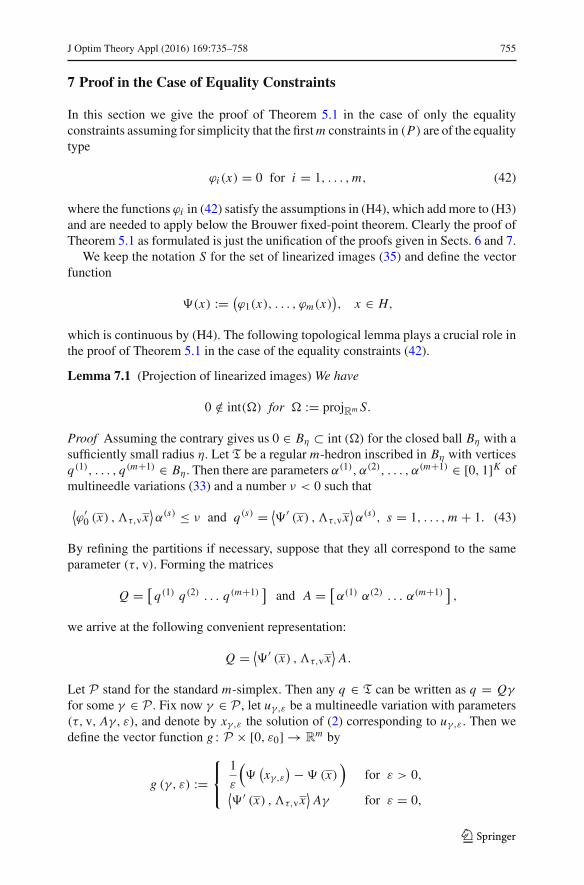
7 Proof in the Case of Equality Constraints

In this section we give the proof of Theorem 5.1 in the case of only the equalityconstraints assuming for simplicity that the firstm constraints in (P) are of the equalitytype

ϕi (x) = 0 for i = 1, . . . , m, (42)

where the functions ϕi in (42) satisfy the assumptions in (H4), which addmore to (H3)and are needed to apply below the Brouwer fixed-point theorem. Clearly the proof ofTheorem 5.1 as formulated is just the unification of the proofs given in Sects. 6 and 7.

We keep the notation S for the set of linearized images (35) and define the vectorfunction

(x) := (ϕ1(x), . . . , ϕm(x))

, x ∈ H,

which is continuous by (H4). The following topological lemma plays a crucial role inthe proof of Theorem 5.1 in the case of the equality constraints (42).

Lemma 7.1 (Projection of linearized images) We have

0 /∈ int(�) for � := projRm S.

Proof Assuming the contrary gives us 0 ∈ Bη ⊂ int (�) for the closed ball Bη with asufficiently small radius η. Let T be a regular m-hedron inscribed in Bη with verticesq(1), . . . , q(m+1) ∈ Bη. Then there are parameters α(1), α(2), . . . , α(m+1) ∈ [0, 1]K ofmultineedle variations (33) and a number ν < 0 such that

⟨

ϕ′0 (x) ,�τ,vx

⟩

α(s) ≤ ν and q(s) = ⟨ ′ (x) ,�τ,vx⟩

α(s), s = 1, . . . , m + 1. (43)

By refining the partitions if necessary, suppose that they all correspond to the sameparameter (τ, v). Forming the matrices

Q = [q(1) q(2) . . . q(m+1)]

and A = [α(1) α(2) . . . α(m+1)]

,

we arrive at the following convenient representation:

Q = ⟨ ′ (x) ,�τ,vx⟩

A.

Let P stand for the standard m-simplex. Then any q ∈ T can be written as q = Qγ

for some γ ∈ P . Fix now γ ∈ P , let uγ,ε be a multineedle variation with parameters(τ, v, Aγ, ε), and denote by xγ,ε the solution of (2) corresponding to uγ,ε. Then wedefine the vector function g : P × [0, ε0] → R

m by

g (γ, ε) :=⎧

⎨

⎩

1

ε

(

(

xγ,ε

)− (x))

for ε > 0,⟨

′ (x) ,�τ,vx⟩

Aγ for ε = 0,

123


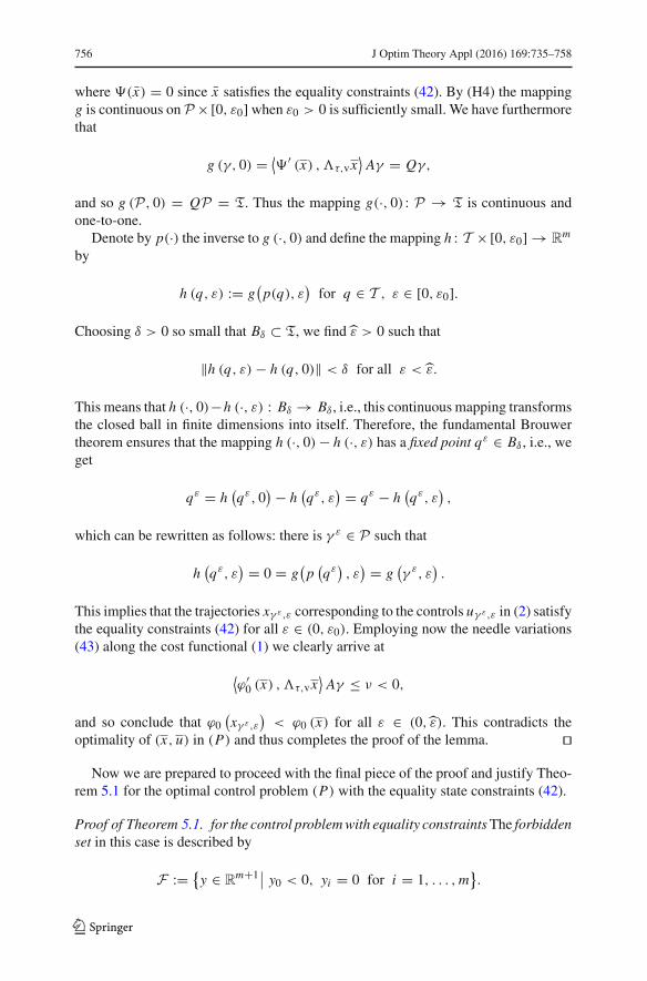
where (x) = 0 since x satisfies the equality constraints (42). By (H4) the mappingg is continuous onP × [0, ε0] when ε0 > 0 is sufficiently small. We have furthermorethat

g (γ, 0) = ⟨ ′ (x) ,�τ,vx⟩

Aγ = Qγ,

and so g (P, 0) = QP = T. Thus the mapping g(·, 0) : P → T is continuous andone-to-one.

Denote by p(·) the inverse to g (·, 0) and define the mapping h : T × [0, ε0] → Rm

by

h (q, ε) := g(

p(q), ε)

for q ∈ T , ε ∈ [0, ε0].

Choosing δ > 0 so small that Bδ ⊂ T, we find ε > 0 such that

‖h (q, ε) − h (q, 0)‖ < δ for all ε < ε.

This means that h (·, 0)−h (·, ε) : Bδ → Bδ , i.e., this continuous mapping transformsthe closed ball in finite dimensions into itself. Therefore, the fundamental Brouwertheorem ensures that the mapping h (·, 0) − h (·, ε) has a fixed point qε ∈ Bδ , i.e., weget

qε = h(

qε, 0)− h

(

qε, ε) = qε − h

(

qε, ε)

,

which can be rewritten as follows: there is γ ε ∈ P such that

h(

qε, ε) = 0 = g

(

p(

qε)

, ε) = g

(

γ ε, ε)

.

This implies that the trajectories xγ ε,ε corresponding to the controls uγ ε,ε in (2) satisfythe equality constraints (42) for all ε ∈ (0, ε0). Employing now the needle variations(43) along the cost functional (1) we clearly arrive at

⟨

ϕ′0 (x) ,�τ,vx

⟩

Aγ ≤ ν < 0,

and so conclude that ϕ0(

xγ ε,ε

)

< ϕ0 (x) for all ε ∈ (0, ε). This contradicts theoptimality of (x, u) in (P) and thus completes the proof of the lemma. ��

Now we are prepared to proceed with the final piece of the proof and justify Theo-rem 5.1 for the optimal control problem (P) with the equality state constraints (42).

Proof of Theorem 5.1. for the control problem with equality constraintsThe forbiddenset in this case is described by

F := {y ∈ Rm+1

∣

∣ y0 < 0, yi = 0 for i = 1, . . . , m}

.

123


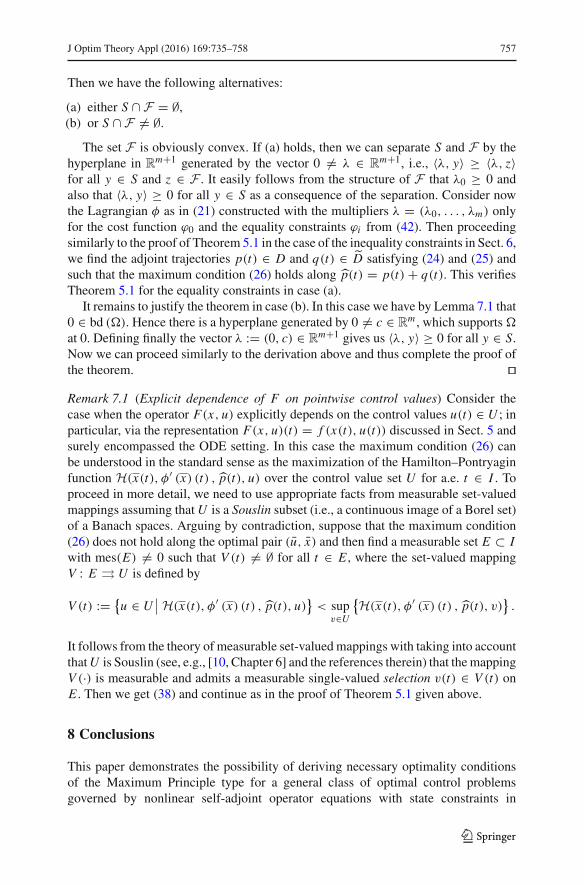
Then we have the following alternatives:

(a) either S ∩ F = ∅,(b) or S ∩ F = ∅.

The set F is obviously convex. If (a) holds, then we can separate S and F by thehyperplane in R

m+1 generated by the vector 0 = λ ∈ Rm+1, i.e., 〈λ, y〉 ≥ 〈λ, z〉

for all y ∈ S and z ∈ F . It easily follows from the structure of F that λ0 ≥ 0 andalso that 〈λ, y〉 ≥ 0 for all y ∈ S as a consequence of the separation. Consider nowthe Lagrangian φ as in (21) constructed with the multipliers λ = (λ0, . . . , λm) onlyfor the cost function ϕ0 and the equality constraints ϕi from (42). Then proceedingsimilarly to the proof of Theorem 5.1 in the case of the inequality constraints in Sect. 6,we find the adjoint trajectories p(t) ∈ D and q(t) ∈ ˜D satisfying (24) and (25) andsuch that the maximum condition (26) holds along p(t) = p(t) + q(t). This verifiesTheorem 5.1 for the equality constraints in case (a).

It remains to justify the theorem in case (b). In this case we have by Lemma 7.1 that0 ∈ bd (�). Hence there is a hyperplane generated by 0 = c ∈ R

m , which supports �

at 0. Defining finally the vector λ := (0, c) ∈ Rm+1 gives us 〈λ, y〉 ≥ 0 for all y ∈ S.

Now we can proceed similarly to the derivation above and thus complete the proof ofthe theorem. ��Remark 7.1 (Explicit dependence of F on pointwise control values) Consider thecase when the operator F(x, u) explicitly depends on the control values u(t) ∈ U ; inparticular, via the representation F(x, u)(t) = f (x(t), u(t)) discussed in Sect. 5 andsurely encompassed the ODE setting. In this case the maximum condition (26) canbe understood in the standard sense as the maximization of the Hamilton–Pontryaginfunction H(x(t), φ′ (x) (t) , p(t), u) over the control value set U for a.e. t ∈ I . Toproceed in more detail, we need to use appropriate facts from measurable set-valuedmappings assuming that U is a Souslin subset (i.e., a continuous image of a Borel set)of a Banach spaces. Arguing by contradiction, suppose that the maximum condition(26) does not hold along the optimal pair (u, x) and then find a measurable set E ⊂ Iwith mes(E) = 0 such that V (t) = ∅ for all t ∈ E , where the set-valued mappingV : E ⇒ U is defined by

V (t) := {u ∈ U∣

∣ H(x(t), φ′ (x) (t) , p(t), u)}

< supv∈U

{

H(x(t), φ′ (x) (t) , p(t), v)}

.

It follows from the theory of measurable set-valued mappings with taking into accountthatU is Souslin (see, e.g., [10, Chapter 6] and the references therein) that themappingV (·) is measurable and admits a measurable single-valued selection v(t) ∈ V (t) onE . Then we get (38) and continue as in the proof of Theorem 5.1 given above.

8 Conclusions

This paper demonstrates the possibility of deriving necessary optimality conditionsof the Maximum Principle type for a general class of optimal control problemsgoverned by nonlinear self-adjoint operator equations with state constraints in

123


infinite-dimensional spaces. Among important and challenging problems of the futureresearch, we mention the following:

(i) To clarify the validity of the technical assumption (H5) for particular classes ofpreudodifferential operator equations as well as functional differential, partialdifferential, integral and other types of equations besides those mentioned above.

(ii) To explore the possibility of extending the results obtained here to the case ofnondifferentiable initial data in optimal control problems.

(iii) To replace the one-dimensional interval I ⊂ R in the optimal control problem (P)

formulated in Sect. 5 by a multidimensional region� ⊂ Rn . It seems that we can

proceed in the later case with constructing “needle-type” variations of controlsand thus make it possible to incorporate the general results of nonlinear operatortheory discussed in Sects. 1–4 to the scheme of deriving necessary optimalityconditions developed in Sects. 5–7.

Acknowledgments The authors thank the King Fahd University of Petroleum and Minerals for excellentfacilities provided to support scientific research. We are indebted to two anonymous referees for theircareful reading the original manuscript and providing many suggestions and remarks, which allowed us tosignificantly improve the original presentation.

References

1. Polak, E.: Optimization: Algorithms and Consistent Approximations. Springer, New York (1997)2. Pontryagin, L.C., Boltyanskii, V.G., Gamkrelidze, R.V., Mishchenko, E.F.: The Mathematical Theory

of Optimal Processes. Wiley, New York (1962)3. Neimark, M.A.: Linear Differential Operators: Part II. Frederick Ungar, New York (1968)4. Warga, J.: OptimalControl ofDifferential and Functional Equations.Academic Press,NewYork (1972)5. Brézis, H.: Operateurs Maximauz Monotones et Semi-Groupes de Contractions dans les Espaces de

Hilbert. North-Holland, Amsterdam (1973)6. Lasiecka, I., Triggiani, R.: Control Theory for Partial Differential Equations. Cambridge University

Press, Cambridge (2000)7. Li, X., Yong, J.: Optimal Control Theory for Infinite-Dimensional Systems. Birkhäuser, Boston (1995)8. Shubin, M.A.: Preudodifferential Operators and Spectral Theory, 2nd edn. Springer, New York (2001)9. Giannessi, F.: Constrained Optimization and Image Space Analysis. Springer, Berlin (2005)

10. Mordukhovich, B.S.: Variational Analysis and Generalized Differentiation, II: Applications. Springer,Berlin (2006)

11. El-Gebeily, M.A., Mordukhovich, B.S., Alshahrani, M.M.: Optimal control of self-adjoint nonlinearoperator equations in Hilbert spaces. Appl. Anal. 93, 210–222 (2014)

12. Alshahrani, M.M., El-Gebeily, M.A., Mordukhovich, B.S.: Maximum principle in optimal control ofsingular ordinary differential equations in Hilbert spaces. Dyn. Syst. Appl. 21, 219–234 (2012)

13. McShane, E.J.: Necessary conditions for generalized curve problems in the calculus of variations.Duke Math. J. 7, 1–27 (1940)

123

Optimal Control of Constrained Self-Adjoint Nonlinear ...€¦ · J Optim Theory Appl (2016)...

Documents

Transcript of Optimal Control of Constrained Self-Adjoint Nonlinear ...€¦ · J Optim Theory Appl (2016)...