By Cahit TASKIN MGIS 410 ELECTRONIC COMMERCE INFRASTRUCTURE AND MANAGEMENT.

Optimal Berth Allocation and Time-Invariant Quay Crane
Assignment in Container Terminals
Yavuz B. Turkogulları
Dept. of Industrial Eng., Maltepe University, Istanbul, Turkey
Z. Caner Taskın, Necati Aras∗, and I. Kuban Altınel
Dept. of Industrial Eng., Bogazici University, 34342, Istanbul, Turkey
Abstract
Due to the dramatic increase in the world’s container traffic, the efficient management of
operations in seaport container terminals has become a crucial issue. In this work, we focus on
the integrated planning of the following problems faced at container terminals: berth allocation,
quay crane assignment (number), and quay crane assignment (specific). First, we formulate a
new binary integer linear program for the integrated solution of the berth allocation and quay
crane assignment (number) problems called BACAP. Then we extend it by incorporating the
quay crane assignment (specific) problem as well, which is named BACASP. Computational
experiments performed on problem instances of various sizes indicate that the model for BA-
CAP is very efficient and even large instances up to 60 vessels can be solved to optimality.
Unfortunately, this is not the case for BACASP. Therefore, to be able to solve large instances,
we present a necessary and sufficient condition for generating an optimal solution of BACASP
from an optimal solution of BACAP using a post-processing algorithm. In case this condition
is not satisfied, we make use of a cutting plane algorithm which solves BACAP repeatedly by
adding cuts generated from the optimal solutions until the aforementioned condition holds. This
method proves to be viable and enables us to solve large BACASP instances as well. To the
best of our knowledge, these are the largest instances that can be solved to optimality for this
difficult problem, which makes our work applicable to realistic problems.
Keywords: berth allocation, crane assignment, container terminals, cutting plane algorithm
1 Introduction
The proportion of containerized trade in the world’s total dry cargo has increased from 5.1% in
1980 to 25.4% in 2008 (UNCTAD, 2009). Containers provide a reliable and standardized means of
transportation, which results in shorter transit times, possibility of using multiple modalities and
∗Corresponding author. E-mail address: [email protected], phone: ++90-212-3597506, fax: ++90-212-2651800.
1

eventually in reduced shipping and handling costs. As a result of these factors, container traffic
has increased by 53.3% between years 2000 and 2010, 11% of which is attributed to year 2010
alone (UNCTAD, 2010). This rate of increase has made efficient management of container terminal
operations crucial, resulting in a significant amount of research from an Operations Research point
of view (Steenken et al., 2004; Stahlbock and Voß, 2008). Container terminal operations are very
complicated, requiring close coordination of ships, cranes, trucks, storage space and personnel. Huge
data and computational resource requirements make it impractical to consider decision problems
on the entire set of operations at once. Instead, container terminal operations are typically grouped
as seaside, transfer and yard operations and the corresponding problems are investigated separately
(Vis and de Koster, 2003). In this paper, we concentrate on integrated seaside operations (Meisel,
2009), and refer the reader to the recent work of Vacca (2010) for more information about transfer
and yard operations.
Various problems in seaside operations have been investigated in the literature. One of the first
lines of research on analysis of seaside operations investigates the applications of queuing models in
port investment decisions for container berths (Edmond and Maggs, 1978). However, more recent
research on seaside operations has focused on solving operational planning problems. In particular,
the berth assignment problem (BAP) deals with the determination of optimal berthing times and
locations of ships such that incoming vessels arrive and depart within their allowed time windows
and no two vessels occupy the same berth-time segment simultaneously (Lai and Shih, 1992; Brown
et al., 1994). The quay crane assignment problem (CAP) deals with allocating cranes to vessels
such that each vessel is assigned to a number of cranes within some specified bounds, and the total
number of cranes is not exceeded (Steenken et al., 2004). CAP can be extended in such a way that
the specific cranes used for the service of vessels are also determined. This problem is referred to as
CAP(specific) in Bierwirth and Meisel (2010), which we name as CASP. This means that in addition
to the number of cranes assigned to a vessel, it is also determined in CASP which individual quay
cranes serve that vessel. More detailed constraints regarding physical alignment of cranes along a
rail are considered as well (Daganzo, 1989; Peterkofsky and Daganzo, 1990). We refer the reader
to Bierwirth and Meisel (2010) for a detailed literature survey on seaside operations.
BAP and CASP can be solved sequentially as suggested by the initial research. However, the
distribution of cranes to vessels has a direct effect on the vessels’ processing times. Therefore, later
research has focused on integrating these problems. To the best of our knowledge, first attempts
for integration are due to Daganzo (1989), and Peterkofsky and Daganzo (1990), where the authors
unify CAP and quay crane scheduling problem (CSP) called CACSP. The aim of CSP is to find a
detailed schedule for each crane by taking into account all unloading and loading operations with
task precedence constraints. Recently, Tavakkoli-Moghaddam et al. (2009) propose a new mixed-
integer programming formulation and a heuristic solution algorithm for CACSP. The integration
of BAP and CAP into berth allocation and quay crane assignment problem (BACAP) has received
more attention (Blazewicz et al., 2011; Bierwirth and Meisel, 2010; Meisel and Bierwirth, 2005,
2009a,b; Hendriks et al., 2008; Giallombardo et al., 2010; Liang et al., 2008). In addition to
proposing solution algorithms for BACAP, Park and Kim (2003) and Imai et al. (2008) propose
2

post-processing approaches for the determination of the specific cranes used. Rashidi (2006) and
Theofanis et al. (2007) develop an integrated mathematical programming formulation for BACAP
that yields the optimal berthing times and positions of the vessels in addition to the number of
cranes.
The BACAP model proposed in Liu et al. (2006) is weaker in the sense that the authors deter-
mine optimal vessel berthing times, crane numbers and specifications, but an optimal solution does
not include any information about berthing positions. Besides, they preprocess CSP to generate
possible handling times for each vessel and each assignable number of cranes. The same approach
is adopted by Meier and Schumann (2007), Meisel (2009), Meisel and Bierwirth (2013) and Ak
(2008). Meier and Schumann (2007) try to achieve this by functionally integrating their integrated
CACSP model with BAP. However, Meisel (2009) and Meisel and Bierwirth (2013) functionally
integrate BACAP with CSP: crane schedules are determined according to the berthing times while
crane assignments are obtained by solving an integrated BACAP model. In his work on the op-
timal planning of the seaside operations, Ak (2008) develops a mixed-integer linear programming
(MILP) model that integrates BAP, CAP and CSP. His model calculates optimal berthing times,
berth allocations and crane number assignments of the vessels, and crane schedules simultaneously
for given specific crane assignments, which makes the presented integration as the deepest of the
available ones. However, the author suggests a Tabu search heuristic since his model can only han-
dle very small problem instances. Zhang et al. (2010) focuses on the integration of BAP and CASP
(which we call BACASP in the sequel). Due to the complexity of their formulation, a commercial
solver package for MILP problems can only deal with up to three vessels within 1 one hour of CPU
time. Therefore, the authors apply a method based on Lagrangean relaxation and sub-gradient
optimization to solve the problem.
In this work we follow this line of research and formulate two new MILP formulations deeply
integrating first BAP and CAP (BACAP), and then BAP and CASP (BACASP). Both of them
consider a continuous berth layout where vessels can berth at arbitrary positions within the range of
the quay and dynamic vessel arrivals where vessels cannot berth before the expected arrival time.
The crane work plan found by solving the BACASP formulation determines the specific crane
allocation to vessels for every time period. As a result, BACASP may be seen as a deep integration
of BAP and CASP for which there is no study according to the recent survey of Bierwirth and
Meisel (2010). In the work plan obtained by solving the BACASP model, when two vessels are
at the berth at the same time, cranes are assigned to vessels in such a way that the one having a
position before the other gets cranes such that the cranes of the former are positioned before those
of the latter. We propose a necessary and sufficient condition for obtaining an optimal solution of
BACASP from an optimal solution of BACAP by a post-processing algorithm. We also develop an
exact solution algorithm for the case where this condition is not satisfied. This is a cutting plane
algorithm that generates cuts for the BACAP formulation until the condition is satisfied. Then
it becomes possible to apply the aforementioned post-processing algorithm and obtain an optimal
solution of BACASP. Experiments show that cutting plane algorithm finds optimal solutions for
problem instances containing up to sixty vessels. To the best of our knowledge, these are the largest
3

instances solved to optimality in the literature, which makes our work applicable for the solution
of real-life problems.
The next section is devoted to the formulations of the new models. We present the new necessary
and sufficient condition for generating a regular work plan from an optimal solution of BACAP
and propose a simple post-processing procedure in Section 3. In Section 4 we present the new
cutting plane algorithm that gives the optimal solution of BACASP. Section 5 reports the results
of the computational study we perform with the new formulations, post-processing procedure and
the new cutting plane algorithm. Finally, concluding remarks are given in Section 6.
2 Model Formulation
Before describing our mathematical formulations for BACAP and BACASP, we will first discuss
the underlying assumptions of our models, which are given as follows:
1. The planning horizon is divided into equal-sized time periods.
2. Crane relocation time is negligible since the length of each time period is much larger than
the crane relocation time.
3. The berth is divided into equal-sized berth sections.
4. Each berth section is occupied by no more than one vessel in each time period.
5. Each quay crane can be assigned to at most one vessel per time period.
6. Each vessel has a minimum and maximum number of quay cranes that can be assigned to it.
7. The service of a vessel by quay cranes begins upon that vessel’s berthing at the terminal, and
it is not disrupted until the vessel departs.
8. The number of quay cranes assigned to a vessel does not change during its stay at the berth,
which is referred to as a time-invariant assignment (Bierwirth and Meisel, 2010). Furthermore,
the set of specific cranes assigned to a vessel is kept the same.
Assumptions 1 through 7 are quite common in the literature as far as BAP and BASP problems
are considered. There are different assumptions, however, regarding the number of cranes assigned
to a vessel during the time the vessel is at the berth. Some authors assume that the number of
cranes may change dynamically between the minimum and maximum number of cranes (see, e.g.
Park and Kim (2003); Meisel and Bierwirth (2009b)), and some others allow a limited number
of changes (Zhang et al., 2010). There are also approaches as the one by Giallombardo et al.
(2010), which can be seen as a compromise between these two modeling assumptions, where the
authors introduce quay crane assignment profiles that represent the number of cranes available to
a vessel during a work shift. These profiles help to consider a limited number of changes (one or
two) in the number of cranes across work shifts. However, the set of profiles has to be known a
priori for each vessel and an increase in their number has a substantial effect on the size of the
4

model. Indeed, the resulting MILP model developed by Giallombardo et al. (2010) becomes hardly
solvable even for small instances as the authors point out in their paper. Therefore, they resort
to a Tabu search heuristic for generating feasible solutions. In our model, quay crane assignment
profiles could be potentially combined with assumption 2 about the negligibility of crane relocation
time to partially relax assumption 8, but this unfortunately yields a different formulation with the
additional binary variables related to assignment of profiles to vessels. The number of these binary
variables is inevitably huge depending the on the number of profiles, which gives rise to the fact
the resulting model cannot be solved efficiently to optimality. As a result, although Assumption
8 appears to be restrictive, it allows us not only to reduce large setup losses due to reallocation
of quay cranes, but also results in an MILP model that can be solved exactly for large instances.
Last but not least, although we do not explicitly consider decreasing crane productivity rates in
our paper, we prefer not to state this fact as a separate assumption because it can be addressed
to a certain extent through parameter pki , which is the processing time of vessel i if k cranes are
assigned to it.
Table 1 lists the parameters used in our mathematical models for BACAP and BACASP along
with their brief descriptions. Similarly, Table 2 displays the decision variables. We will next discuss
the details of our solution approaches.
2.1 Berth and Quay Crane Allocation Problem (BACAP)
As described in Section 1, BACAP is an extension of the berth allocation problem (BAP), in
which the (aggregate) capacity of quay cranes is considered. BACAP aims to find optimal berthing
sections and berthing times of vessels as well as the number of cranes assigned to each vessel so as
to minimize the total cost.
Let us define a binary variable Xkijt, which is equal to one if vessel i starts berthing at section j
in time period t, and k quay cranes are assigned to it, and zero otherwise. Constraint (1) ensures
that each vessel berths at a unique section and time period, and the number of quay cranes assigned
to it lies between the minimum and maximum allowed quantities:
B−`i+1∑j=1
ki∑
k=ki
T−pki +1,∑t=ei
Xkijt = 1 i = 1, . . . , V. (1)
The next set of constraints eliminates overlaps between vessels at the berth. In particular, constraint
set (2) guarantees that each berth section is occupied by at most one vessel in each time period
(see Assumption 4). To put it differently, there should not be any overlap among the rectangles
representing vessels in the two-dimensional time-berth section space, which are located between
max(ei, t− pki + 1
)and min
(T − pki + 1, t
)on the time dimension, and between max
(1, j − `i + 1
)and min
(B − `i + 1, j
)on the berth section dimension.
V∑i=1
min(B−`i+1,j)∑j=max(1,j−`i+1)
ki∑
k=ki
min(T−pki +1,t)∑t=max(ei,t−pki +1)
Xkijt ≤ 1 j = 1, . . . , B; t = 1, . . . , T (2)
5

Table 1: Parameters used in mathematical models.
Parameter Definition
i Index of vessels
g Index of crane groups
j Index of berth sections
k Index of crane numbers
t Index of time periods
B Number of berth sections
C(g) Index set of cranes in group g
G Number of crane groups
N Number of available quay cranes
T Number of time periods in the planning horizon
V Number of vessels
cgl Index of the leftmost crane in group g
cgr Index of the rightmost crane in group g
di Due time of vessel i
ei Arrival time of vessel i
ki Lower bound on the number of cranes that can be assigned to vessel i
ki
Upper bound on the number of cranes that can be assigned to vessel i
`i Length of vessel i
pki Processing time of vessel i if k cranes are assigned to it
si Desired berth section of vessel i
φi1 Cost of one unit deviation from the desired berth section for vessel i
φi2 Cost of berthing one period later than the arrival time for vessel i
φi3 Cost of departing one period later than the due time for vessel i
Table 2: Decision variables used in mathematical models.
Decision Variables Definition
Xkijt 1 if vessel i berths at section j in time period t and k quay cranes are
assigned to it, 0 otherwise
Y git 1 if crane group g starts serving vessel i in time period t, 0 otherwise
Zct position of crane c in time period t
Constraint sets (1) and (2) represent the feasible region of BAP. We next discuss how quay
crane availability can be handled in the BACAP model. Let us denote the number of available
quay cranes by N . Constraint set (3) ensures that in each time period the number of active quay
6

cranes is less than or equal to the available number of cranes:
V∑i=1
B−`i+1∑j=1
ki∑
k=ki
min(T−pki +1,t)∑t=max(ei,t−pki +1)
kXkijt ≤ N t = 1, . . . , T (3)
The objective function (4) of our model minimizes the total cost, whose components for each
vessel are: i) the cost of deviation from the desired berth section, ii) the cost of berthing later than
the arrival time, and iii) the cost of departing later than the due time. Our integer programming
formulation for BACAP can be summarized as follows:
min
V∑i=1
ki∑
k=ki
B−`i+1∑j=1
T−pki +1∑t=ei
{φi1|j − si|+ φi2 (t− ei) + φi3 max
(0, t+ pki − 1− di
)}Xk
ijt (4)
subject to: constraints (1), (2), (3)
Xkijt ∈ {0, 1} i = 1, . . . , V ; j = 1, . . . , B − `i + 1; k = ki, . . . , k
i; t = ei, . . . , T − pki + 1.
A compact presentation of the formulation is included in the appendix. In this formulation, the
cost of berthing away from the desired berthing position is a linear function of the deviation from
the desired berthing position. When a vessel is berthed away from its desired berthing position,
the distance to the storage area in the yard, where containers are stored, also increases. This may
require the use of additional transport vehicles, which increases the corresponding cost. In case
this cost component is a nonlinear function of the deviation, then the model can easily be modified
by revising the term φi1|j − si|. This is possible since this term is a parameter and represents a
coefficient of the decision variable Xkijt in the objective function (4). As a matter of fact, the way
the decision variable is defined in the model above makes the definition of cost components quite
flexible. The other two cost components are related to late arrival and departure of vessels. The
terms φi2 (t− ei) and φi3 max(0, t+ pki − 1− di
)represent the penalties associated with berthing
and departure delays, respectively, where the unit cost parameters φi2 and φi3 are mostly specified
in the contracts between the terminal operators and liner shipping companies. This is the form of
objective function commonly used in the literature (e.g., Zhang et al. (2010)).
Note that our model contains O(NVBT ) binary variables and O(V +BT ) constraints. Although
it contains a significant number of binary variables, we observe that constraint set (1) exposes a set
partitioning structure while constraint set (2) exhibits a set packing structure in the formulation.
Furthermore, both constraint sets define specially ordered sets of type 1 (SOS1) whose special
structure can be exploited by integer programming solvers for efficient branching (Nemhauser and
Wolsey, 1988). Therefore, even though our formulation contains a large number of binary variables,
it has a special form that increases the efficiency of the solution procedure. We should emphasize,
however, that all these computationally favorable properties of the mathematical model are due to
assumption 8 about the time-invariant crane assignments. Therefore, its relaxation to make the
model more realistic with time-variant crane assignments would also destroy the special structure
of the formulation.
7

2.2 Berth Allocation and Quay Crane Assignment (Specific) Problem (BA-
CASP)
Recall that although the availability of quay cranes is considered in constraint set (3) in BACAP,
it is not determined which particular crane is assigned to which vessel in a given time period, and
thus the working periods of the cranes are unknown. Therefore, it would not be surprising that
a feasible solution of BACAP yields an infeasible assignment for some or all of the cranes, which
necessitates additional crane movements during which the service on some vessels is disrupted. For
the clarification of this issue, consider an example with three vessels and 12 quay cranes. Table 3
includes the data associated with this small problem. Note that the length of each vessel is five
units in terms of the number of berth sections and six cranes have to be assigned to each vessel
in each time period. The vessels have different desired berth sections (si), arrival times (ei), due
times (di) and processing times (pki ). An optimal solution of this BACAP instance is depicted in
Figure 1.
Table 3: The data for the sample problem instance.
Vessel `i ki ki si ei di pki φi1 φi2 φi3
1 5 6 6 1 5 120 30 1000 1000 2000
2 5 6 6 10 20 130 40 1000 1000 2000
3 5 6 6 16 45 140 50 1000 1000 2000
Figure 1: An optimal solution of the sample BACAP instance given in Table 3.
In this figure, the x-axis and y-axis represent, respectively, the time periods and the berth
sections. Each vessel is displayed as a rectangle. In particular, Vessel 1 is assigned to berth section
1 in period 5. Since its processing time is 30 periods and its length is 5 units, it occupies the area
designated by V1 in the two-dimensional time-berth section space. Note that each vessel is associ-
ated with a unique combination of berth section, time period, and number of cranes (constraint set
(1)), and none of the rectangles overlaps with another one (constraint set (2)). Moreover, no more
than 12 quay cranes are required in any period (constraint set (3)). In fact, between periods 5 and
8
19 when vessel 1 is at the berth, six cranes are needed, while 12 cranes are used between periods
20 and 34 since both vessel 1 and vessel 2 are at the berth. From period 35 to period 44, again
six cranes are required to serve vessel 2, while 12 cranes have to be in charge between periods 45
and 59 because vessel 2 and vessel 3 are together at the berth. Finally, the service for vessel 3 is
performed by six cranes between periods 60 and 94. Although no more than 12 cranes are required
in any period, it is not possible to assign the cranes without making a change in the group of cranes
that serves each vessel or moving some of the cranes over some others to change their relative order.
Both of these operations require setup and hence a delay in the service provided to the vessels. For
example, if cranes indexed 1–6 are assigned to vessel 1 and cranes 7–12 are assigned to vessel 2,
the first crane group has to be used for vessel 3 as well, but this requires the change of the relative
order of cranes 1–6 with respect to cranes 7–12, i.e., the former group must be positioned after
the latter group. This implies that a feasible solution to BACAP is not necessarily feasible for
BACASP. Note, however, that all feasible solutions of BACASP are feasible for BACAP.
To develop a mathematical programming formulation for BACASP we extend the formulation
for BACAP by including the constraint sets (1)–(3) and defining new variables and constraints so
that feasible specific crane assignments are obtained for quay cranes, which do not incur setup due
to the change in the relative order of cranes. We should remark that if quay cranes i− 1 and i+ 1
are assigned to a vessel in a time period, then quay crane i has to be assigned to the same vessel as
well since quay cranes are located along the berth on a single railway. In order to incorporate this
requirement, we define a crane group as a set of adjacent quay cranes and let the binary variable
Y git denote whether crane group g assigned to vessel i starts service in time period t. Constraint set
(5) relates the X and Y-variables. It ensures that if k quay cranes are assigned to vessel i, it must
be served by a crane group g that is formed by |C(g)| = k adjacent cranes, where C(g) is the index
set of cranes in group g and | · | denotes the cardinality of a set. Moreover, G is the total number
of crane groups.
B−`i+1∑j=1
Xkijt −
G∑g=1|C(g)|=k
Y git = 0 i = 1, . . . , V ; k = ki, . . . , k
i; t = ei, . . . , T − pki + 1 (5)
Notice that in constraints (5), C(g)’s are pre-determined and hence are parameters of the model.
For example, if N = 3, the size of possible crane groups can be one, two, or three, and the total
number of crane groups G = 6. Crane groups of size one, i.e. crane groups consisting of one crane,
are C(g = 1) = {1}), C(g = 2) = {2}), C(g = 3) = {3}). Similarly, crane groups of size two are
C(g = 4) = {1, 2}) and C(g = 5) = {2, 3}). It is important to point out that C(g) = {1, 3}) is not
a valid group because cranes 1 and 3 are not adjacent. Finally, there is only one crane group of size
three, namely C(g = 6) = {1, 2, 3}). It should be emphasized that each crane can be a member of
multiple crane groups. However, each crane can operate as a member of at most one group in each
time period. The next set of constraints (6) guarantees that this condition holds:
9

V∑i=1
G∑g=1
c∈C(g)
min(T−pki +1,t)∑t=max(ei,t−pki +1)
Y git ≤ 1 c = 1, . . . , N ; t = 1, . . . , T (6)
Even though constraints (5) and (6) make sure that each quay crane is assigned to at most one
vessel in any time period (Assumption 5), they do not guarantee that quay cranes are assigned to
vessels in the correct sequence. In particular, let the quay cranes be indexed in such a way that
a crane positioned closer to the beginning of the berth has a lower index. Also, without loss of
generality, we can assume that the berth sections are oriented horizontally from left to right. This
implies that a crane having a smaller index is located on the left-hand side of another crane with
a larger index. Since all cranes perform their duty along a rail at the berth, they cannot pass each
other or stated differently their order cannot be changed. The next four constraint sets help to
ensure preserving the crane ordering. Here, Zct denotes the position of crane c in time period t.
Zct ≤ Z(c+1)t c = 1, . . . , N − 1; t = 1, . . . , T (7)
ZNt ≤ B t = 1, . . . , T (8)
Zcgl t+B(1− Y g
it ) ≥B−`i+1∑
j=1
ki∑
k=ki
jXkijt i = 1, . . . , V ; g = 1, . . . , G; t = ei, . . . , T − pki + 1;
t ≤ t ≤ t+ pki − 1 (9)
Zcgrt≤
B−`i+1∑j=1
ki∑
k=ki
(j + `i − 1)Xkijt +B(1− Y g
it ) i = 1, . . . , V ; g = 1, . . . , G; t = ei, . . . , T − pki + 1;
t ≤ t ≤ t+ pki − 1 (10)
Constraint set (7) simply states that the positions of the cranes (in terms of berth sections) are
respected by the index of the cranes. This means that the position of crane c is always less than
or equal to the position of crane c+ 1 during the planning horizon. Constraint set (8) makes sure
that the last crane (crane N) is positioned within the berth. By defining cgl and cgr as the index of
the crane that is, respectively, the leftmost and rightmost member of crane group g, constraint set
(9) guarantees that if crane group g is assigned to vessel i and vessel i berths at section j, then the
position of the leftmost member of crane group g is greater than or equal to j. Similarly, constraint
set (10) ensures that if crane group g is assigned to vessel i and vessel i berths at section j, then
the position of the rightmost member of crane group g is less than or equal to j + `i − 1, which is
the last section of the berth occupied by vessel i.
We now analyze the set of constraints (1)–(3) and (5)–(10) of BACASP. As a result of this
analysis, we are able to show in Proposition 1 and Proposition 3 that some constraints of BACASP
are in fact implied by the others. We also demonstrate in Proposition 2 that (7)–(10) yield the
desired quay crane sequence.
Proposition 1 Constraint set (3) is implied by constraint sets (5) and (6).
10

Proof. Summing constraints (6) for c = 1, . . . , N , we obtain
V∑i=1
min(T−pki +1,t)∑t=max(ei,t−pki +1)
N∑c=1
G∑g=1
c∈C(g)
Y git ≤ N t = 1, . . . , T. (11)
We observe that the total number of cranes assigned to vessel i in period t can be written in the
following equivalent form:N∑c=1
G∑g=1
c∈C(g)
Y git =
ki∑
k=ki
kG∑
g=1|C(g)|=k
Y git . (12)
Inequality (11) and equality (12) imply together that
V∑i=1
min(T−pki +1,t)∑t=max(ei,t−pki +1)
ki∑
k=ki
k
G∑g=1|C(g)|=k
Y git ≤ N t = 1, . . . , T. (13)
Finally, from (5) and (13) it is possible to obtain
V∑i=1
min(T−pki +1,t)∑t=max(ei,t−pki +1)
ki∑
k=ki
k
B−`i+1∑j=1
Xkijt ≤ N t = 1, . . . , T, (14)
which is equivalent to (3).
Proposition 2 If vessels i1 and i2 are at the berth in time period t and their berthing sections have
the relation j1 ≤ j2, then the index of the leftmost crane assigned to i2 is greater than the index of
the rightmost crane assigned to i1.
Proof. Constraints (9) and (10) imply that
Zcg2l t ≥ j2 (15)
Zcg1r t ≤ j1 + l1 − 1, (16)
where Zcg2l t denotes the position of the leftmost crane of group g2 assigned to vessel i2 and Zc
g1r t
denotes the position of the rightmost crane of group g1 assigned to vessel i1. Recall that no berth
segment can be used by two vessels simultaneously (constraint set (2)). Therefore, the inequality
j2 > j1 + l1 − 1. (17)
is valid. Inequalities (15)–(17) imply that
Zcg2l t > Zc
g1r t. (18)
Finally, inequality (18) together with constraints (7) imply that
cg2
l > cg1
r . (19)
11

Proposition 3 Constraint set (6) is implied by (7), (9) and (10).
Proof. Consider the mathematical model without constraints (6) and assume that a crane is
assigned to more than one vessel in a period. This implies that the two vessels are at the berth in
the same period. However, as a result of Proposition 2, we know that the index of the rightmost
crane assigned to the vessel on the left is strictly smaller than the index of the leftmost crane
assigned to the vessel at the right, which is a contradiction.
As a consequence of these propositions, the mixed-integer linear programming formulation for
BACASP reduces to
minimize (4)
subject to: (1), (2), (5), (7)− (10)
Xkijt ∈ {0, 1} i = 1, . . . , V ; j = 1, . . . , B − `i + 1; k = ki, . . . , k
i; t = ei, . . . , T − pki + 1
Y git ∈ {0, 1} i = 1, . . . , V ; g = 1, . . . , G; t = 1, . . . , T
Zct ≥ 0 c = 1, . . . , N ; t = 1, . . . , T.
In order to increase readability we included a compact presentation of the formulation in the
appendix. As can be observed, this formulation has O(N2V T ) variables and O(N2V T 2) constraints,
which makes our BACASP formulation significantly larger than our BACAP formulation. Hence,
it should be expected that only small BACASP instances can be solved exactly using CPLEX
12.2. As will be demonstrated in the computational study, this is indeed the case and although our
formulation proposed in this paper for the BACASP problem is relatively more efficient than the
other models existing in the literature, it can optimally solve problem instances up to 15 vessels.
Using the formulation of BACAP, on the other hand, we can solve instances up to 60 vessels. This
fact has motivated us to make use of the formulation for BACAP in solving larger sized BACASP
instances to optimality. The next section is the outcome of our efforts towards that goal.
3 Transforming an Optimal Solution for BACAP to an Optimal
Solution of BACASP
By carefully analyzing the optimal solutions of BACAP and BACASP in small sized instances, we
have figured out that an optimal solution of BACASP can be generated from an optimal solution of
BACAP provided that the condition given below in Proposition 4 is satisfied. This amounts to first
solving BACAP optimally, and then finding an optimal solution of BACASP using a polynomial
time algorithm. In case this condition is not satisfied, we devise a cutting plane algorithm in which
the added cuts ultimately yield an optimal BACAP solution satisfying it. The mentioned condition,
which plays a crucial role in our solution procedure, is based on the notion of complete sequence
of vessels (with respect to their occupied berthing positions), which is defined as follows.
Definition 1 A vessel sequence v1, v2, . . . , vn in a given feasible solution of BACAP is complete if
12

i. v1 is the closest vessel to the beginning of the berth,
ii. vn is the closest vessel to the end of the berth,
iii. vi and vi+1 are two consecutive vessels with vi closer to the beginning of the berth,
iv. Two consecutive vessels in this sequence have to be at the berth concurrently during at least
one time period.
A complete sequence is said to be proper when the sum of the number of cranes assigned to vessels
in this sequence is less than or equal to N . Otherwise, it is called an improper complete sequence.
As mentioned before, we assume that a vessel vi is positioned on the left-hand side of another vessel
vj if the former is closer to the beginning of the berth. Figure 2 depicts an optimal BACAP solution
of an instance with 21 vessels considered later in Section 4.1 (more specifically, it is the instance
whose parameter values are provided in Table 5). The number in the parenthesis under the vessel
number within each rectangle gives the number of cranes assigned to the vessel. By analyzing
Figure 2, we find that the vessel sequence {V2,V3,V4} is complete. Similarly, the vessel sequence
{V14,V13,V16} is also complete. There are many other complete sequences in the BACAP solution
shown in this figure. Notice that all of the complete sequences in Figure 2 are proper because the
sum of the number of cranes assigned to the vessels in each sequence is less than or equal to N = 12
as defined later in Section 4.1.
Figure 2: An optimal solution of BACAP for an instance with 21 vessels.
Proposition 4 Given an optimal solution X∗ of BACAP, an optimal solution (X∗,Y∗,Z∗) of
BACASP can be obtained from it if and only if every complete sequence of vessels extracted from
X∗ is proper.
Proof. First we show that if an optimal solution (X∗,Y∗,Z∗) of BACASP can be obtained
from an optimal solution X∗ of BACAP, then every complete sequence of vessels is proper, i.e., the
sum of the number of cranes assigned to vessels in every complete sequence is less than or equal
to N . Suppose that the sum of the number of cranes assigned to vessels in a complete sequence of
vessels v1, v2, . . . , vn is larger than N and θi cranes are assigned to vessel vi in the optimal solution
13

of BACAP. Then, the smallest index of the rightmost crane assigned to vessel v1 is θ1 (i.e., indices
of the cranes assigned to vessel v1 are 1, 2, . . . , θ1). Since v2 is at the berth concurrently with v1 in
at least one time period and v2 is on the right-hand side of v1, the indices of the cranes assigned
to v2 are θ1 + 1, θ1 + 2, . . . , θ1 + θ2. Ultimately, the index of the last crane assigned to vessel vn is
θ1 + θ2 + · · · + θn. Since we know that this quantity is larger than N , such a crane assignment is
not feasible for BACASP.
To show that if every complete sequence of vessels that can be extracted from an optimal
solution X∗ of BACAP is proper, then an optimal solution of BACASP with decision variables
values (X∗,Y∗,Z∗) can be obtained X∗, we make use of a constructive method called Algorithm
1. Note that it is sufficient to show that this algorithm generates a feasible solution (X′,Y′,Z′) for
BACASP because such a solution is also optimal since the objective function of BACASP is the
same as that of BACAP.
In Algorithm 1, VNA denotes the set of vessels to which no cranes are assigned yet and its
complement VA the set of vessels to which cranes are assigned. Clearly, VNA and VA partition the
set of vessels {1, 2, . . . , V }. Notice that the way the vessels are picked up from VNA and added to
the set VA implies that the order of the vessels forms one or more complete sequences in the set
VA. It is also ensured that these complete sequences are proper. Therefore, upon the termination
of Algorithm 1, each vessel is assigned a crane group from the set of available cranes.
Algorithm 1
Initialization: Let VA ← ∅, VNA ← {1, 2, . . . , V }while VNA 6= ∅ do
Select vessel v ∈ VNA that berths in the leftmost berth section
Find the vessels in VA that are at the berth with v in at least one time period. Among the
cranes assigned to these vessels, find the crane cmax that is in the rightmost berth section.
if VA = ∅ or @ any vessel in VA that is at the berth with v in at least one time period then
cmax ← 0
end if
Assign cranes indexed from cmax + 1 to cmax + θv to vessel v.
VA ← V ∪ v, VNA ← VNA \ vend while
Consider two vessels vi and vj that are at the berth in time period t and vi is on the left-hand
side of vj . Due to the selection rule vi is already in the set VA when vj is added to VA. Due to the
assignment rule, the index of the rightmost crane assigned to vessel vi is less than the index of the
leftmost crane assigned to vessel vj . This implies that at the end of Algorithm 1, a particular crane
is assigned to at most one vessel in a given time period. Notice that the assignment of cranes to
vessels using Algorithm 1 does not make any change in the objective function because the berthing
positions and berthing times of the vessels are not modified. Thus the solution given by Algorithm
1 is an optimal solution of BACASP.
14

As a result of Proposition 4, it is possible to obtain an optimal solution of BACASP from an
optimal solution of BACAP using Algorithm 1 provided that every complete sequence of vessels is
proper. From the implementation point of view, determining whether this condition is satisfied or
not requires both the generation of all complete sequences and checking their properness.
3.1 Generating all complete sequences and checking their properness
Let us construct a directed acyclic network in which nodes correspond to vessels. Therefore, we use
the terms “node” and “vessel” interchangeably in the remainder of this subsection. Two dummy
nodes v0 and vn+1 are also added to the graph. There is an arc from node v0 to any other node vi
which corresponds to a vessel with no other vessel on their left-hand side during the time periods it
is at the berth. The weight of this arc is the number of cranes assigned to vessel vi in the optimal
solution of BACAP. In the network, there is also an arc going from node vi to node vj if vi is on
the left-hand side of vj with no vessel in between. The weight of this arc is the number of cranes
assigned to vj in the optimal solution of BACAP. Finally, there is an arc from every node, which
corresponds to a vessel with no other vessel on its right-hand side during the time periods it is
at the berth, to node vn+1, and the weight of this arc is zero. Note that the construction of this
network requires that the order of the vessels from left to right at the berth (or from the beginning
of the berth to the end) in the optimal solution of BACAP be found in each time period.
It is easy to observe that the nodes on each directed path from node v0 to node vn+1 represents
a complete sequence of vessels in this network. Also, each complete sequence corresponds to a path
beginning at node v0 and ending at node vn+1 in the network. Furthermore, the length of each
such path gives the sum of the number of cranes assigned to vessels in the corresponding complete
sequence. As a result, finding the complete sequence with the largest number of cranes amounts to
identifying the longest path in this network, which can be used to check the properness condition in
Proposition 4. If the length of the longest path, i.e., the total number of cranes in the corresponding
complete sequence is less than or equal to N (or equivalently this complete sequence is proper),
then the condition given in the proposition is satisfied and it is possible to generate an optimal
solution for BACASP. Notice that the length of the longest path in a directed acyclic graph can be
found in polynomial time (Ahuja et al., 1993).
To illustrate the idea explained above, consider again the optimal BACAP solution given in
Figure 2. To find out whether it is possible to generate an optimal solution of BACASP from this
optimal solution of BACAP, we construct the directed acyclic graph displayed in Figure 3. Since
the length of the longest path (there exist multiple such paths) in this graph is 12, which is equal
to the number of available cranes N , we can apply Algorithm 1 to generate an optimal solution of
BACASP as shown in Proposition 4. This solution is illustrated in Figure 4.
3.2 A Cutting plane algorithm to optimally solve BACASP
If there is at least one improper complete sequence of vessels in an optimal solution of BACAP,
namely a complete sequence where the sum of the number of cranes assigned to vessels is larger
15

Figure 3: Directed acyclic graph associated with the instance whose BACAP solution is in Figure
2
Figure 4: An optimal solution of BACASP for the instance with 21 vessels.
than N , then we cannot apply Algorithm 1 to obtain an optimal solution of BACASP. In that case,
it is possible to add the cut given in (20) corresponding to an improper complete sequence into the
formulation of BACAP, where IS refers to an improper complete sequence and |IS| is the total
number of vessels in it. Note that this cut is used to eliminate feasible solutions that involve IS.∑i∈IS
Xk(i)ij(i)t(i) ≤ |IS| − 1 (20)
The left-hand side of (20) is the sum of the Xkijt variables which are set to one for the vessels
involved in IS. In other words, there is only one Xkijt = 1 for each vessel i ∈ IS. The j,k, and
t indices for which Xkijt = 1 related to vessel i are denoted as j(i), k(i), and t(i) in (20). Upon
the addition of this cut, BACAP is solved again. The addition of these cuts is repeated until an
16
optimal solution of BACAP does not contain any improper complete sequences. At that instant,
Algorithm 1 can be called to generate an optimal solution of BACASP from the existing optimal
solution of BACAP. As a result, the cutting plane algorithm outlined below as Algorithm 2 can be
used to find an optimal solution of BACASP.
Algorithm 2
Initialization: Let P be the BACAP formulation without any cuts
while There is at least one improper complete sequence in an optimal solution of P do
Generate a cut based on (20) for an improper complete sequence and update P by adding the
cut to it.
Solve P
end while
Run Algorithm 1
In the following example, we explain the procedure of generating the cuts. The vessel-related
parameters of the instance in the example are given in Table 4. As can be seen in this table, two
cranes have to be assigned to every vessel, and processing times p2i are 3,4, and 3, respectively when
two cranes are assigned to the vessels. Moreover, the number of available cranes N is equal to four.
Table 4: Parameters of the sample instance used to illustrate the cutting plane algorithm.
Vessel `i ki ki si ei di pki φi1 φi2 φi3
1 1 2 2 1 1 8 3 1000 1000 2000
2 1 2 2 2 2 8 4 1000 1000 2000
3 1 2 2 3 4 8 3 1000 1000 2000
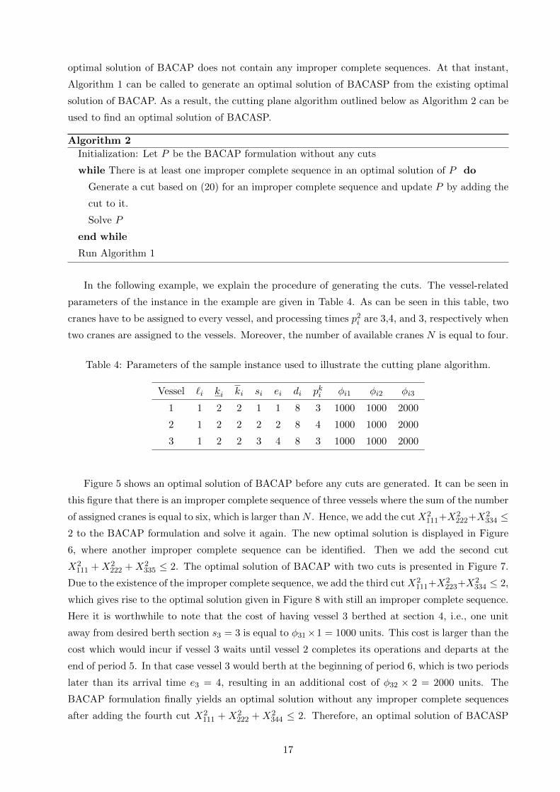
Figure 5 shows an optimal solution of BACAP before any cuts are generated. It can be seen in
this figure that there is an improper complete sequence of three vessels where the sum of the number
of assigned cranes is equal to six, which is larger than N . Hence, we add the cut X2111+X2
222+X2334 ≤
2 to the BACAP formulation and solve it again. The new optimal solution is displayed in Figure
6, where another improper complete sequence can be identified. Then we add the second cut
X2111 + X2
222 + X2335 ≤ 2. The optimal solution of BACAP with two cuts is presented in Figure 7.
Due to the existence of the improper complete sequence, we add the third cutX2111+X2
223+X2334 ≤ 2,
which gives rise to the optimal solution given in Figure 8 with still an improper complete sequence.
Here it is worthwhile to note that the cost of having vessel 3 berthed at section 4, i.e., one unit
away from desired berth section s3 = 3 is equal to φ31×1 = 1000 units. This cost is larger than the
cost which would incur if vessel 3 waits until vessel 2 completes its operations and departs at the
end of period 5. In that case vessel 3 would berth at the beginning of period 6, which is two periods
later than its arrival time e3 = 4, resulting in an additional cost of φ32 × 2 = 2000 units. The
BACAP formulation finally yields an optimal solution without any improper complete sequences
after adding the fourth cut X2111 + X2
222 + X2344 ≤ 2. Therefore, an optimal solution of BACASP
17

can be generated from this optimal solution of BACAP as displayed in Figure 9. Notice that in
this optimal solution vessel 2 is delayed until the departure of vessel 1 with a cost of 2000 units.
An alternative optimal solution is that vessel 2 berths at period 4, which is its arrival time e2 = 2,
but two sections away from its desired berth section s2 = 2 with the same cost of 2000 units. The
only difference between this alternative optimal BACASP solution and the one presented in Figure
9 is that cranes 3 and 4 would be assigned to vessel 2 instead of cranes 1 and 2, and cranes 1 and
2 would be assigned to vessel 3 (after terminating their operation on vessel 1) instead of cranes 3
and 4 in the current optimal solution.
Figure 5: An optimal solution of BACAP for the sample instance before adding cuts.
Figure 6: An optimal solution of BACAP for the sample instance after adding one cut.
Figure 7: An optimal solution of BACAP for the sample instance after adding two cuts.
As can be noticed even in this small instance, after adding a cut to eliminate an improper com-
18

Figure 8: An optimal solution of BACAP for the sample instance after adding three cuts.
Figure 9: An optimal solution of BACASP for the sample instance after adding four cuts.
plete sequence from the feasible region, another improper complete sequence of the same vessels with
different berthing times and/or berthing positions may appear. In order to simultaneously exclude
all feasible solutions with these improper complete sequences, and thus speed up the convergence
of the cutting plane algorithm, we modify it in the following way. When an improper complete
sequence IS is identified, for each vessel i ∈ IS we determine the values of the indices for berthing
section (j), berthing time (t), and the number of cranes (k) such that when Xkijt = 1 for these
(j, t, k) triplets, vessel i continues to remain within IS. Namely, we let Qi = {(j, k, t) : Xkijt = 1}
for i ∈ IS. Then we add the following cut to the BACAP formulation
∑(j,t,k)∈Qi
Xkijt +
∑l∈IS,l 6=i
Xk(l)lj(l)t(l) ≤ |IS| − 1 (21)
for each vessel i ∈ IS, which lifts cut (20). Algorithm 2 remains the same except that multiple
cuts (one for each vessel i) rather than a single cut are added to the BACAP formulation. In the
example, the following three cuts are added right after solving BACAP initially:
X2111 +X2
112 +X2113 +X2
114 +X2115 +X2
222 +X2334 ≤ 2 (23a)
X2222 +X2
223 +X2111 +X2
334 ≤ 2 (23b)
X2334 +X2
344 +X2354 +X2
364 +X2335 +X2
345 +X2355 +X2
365 +X2222 +X2
111 ≤ 2 (23c)
19

Solving BACAP with these cuts immediately provides the optimal solution of BACASP given
in Figure 9. Notice that we solve the BACAP formulation twice as opposed to the previous case
of adding a single cut where five CPLEX calls are necessary. As a second example, we consider
the instance examined before, i.e., the instance with three vessels and 12 quay cranes, whose
parameters were given in Table 3. Recall that for this instance an optimal solution of BACASP
could not be obtained for the optimal solution of BACAP depicted in Figure 1. By implementing
the cutting plane algorithm with single and multiple cuts, the optimal solution of the BACASP
instance can be obtained as shown in Figure 10. In the single cut strategy, the number of improper
complete sequences identified, the number of cuts generated, and the CPU time in seconds are
equal to 11,023, 11,023, and 199,166 seconds, respectively. In the multiple cut strategy, on the
other hand, the corresponding values are 317, 951, and 3946 seconds, respectively. This indicates
that when multiple cuts are used, the number of improper complete sequences detected, which
actually represents the number of 0-1 integer programs solved, is much less than the number of
cuts obtained using the single cut strategy. This also explains why much less computation time is
spent when multiple cuts are generated. Notice that in the optimal solution presented in Figure 10,
vessel 3 berths at section 5, that is 11 sections away from its desired berth section s3 = 16. This is
because of the proper alignment constraints of the quay cranes. As an alternative, vessel 3 could
wait for vessel 2 to terminate its operations and then berth at its desired berth section. However,
doing so would delay its berthing time to period 60 with a 15 periods difference from its arrival
time e3 = 45. The associated cost of berthing 15 periods later than the arrival time amounts to
φ32 × 15 = 15, 000 units that is higher than the cost of berthing 11 berth sections away from the
desired one, which is φ31 × 11 = 11, 000 units. Therefore, vessel 3 is better off if berthed relatively
far from its desired berth section as illustrated in Figure 10.
Figure 10: Optimal solution of the instance given in Table 3 by the cutting plane algorithm.
4 Computational Study
In this section we perform computational experiments on a set of problem instances using our
BACAP and BACASP models. All the experimental study is carried out on a computer with Intel
Xeon 3.16 GHz processor and 130 GB of RAM working under Windows 2003 Server operating
20

system.
4.1 Small and Medium Instances
Our first set of instances consists of seven small and medium instances and they have been derived
from the real data used in Zhang et al. (2010) taken from the Tianjin Five Continents International
Container Terminal in Tianjin, People’s Republic of China. In this real data set, there are 21
vessels and 12 quay cranes where the 1200 meters long berth is divided into 24 berth sections each
of which is 50 m and the planning horizon is 200 hours. The parameters related to the vessels are
given in Tables 5 and 6. Table 5 includes the length of the vessels, the minimum and maximum
number of cranes that can be assigned to each vessel, the desired berth section, the arrival time,
and the due time of each vessel. Table 6 contains the processing time pki of vessel i when k cranes
are assigned to it. They are generated by dividing the total operational time of each vessel, which is
expressed as the number of crane-time periods required to discharge and load all the containers of
that vessel in Zhang et al. (2010), by the number of cranes that can be assigned and rounding up to
the nearest integer. For example, the total operational time of vessel 2 is 96 crane-time periods and
3–6 cranes can be assigned to it; therefore p3i = d96/3e = 32, p4i = d96/4e = 24, p5i = d96/5e = 20,
and p6i = d96/6e = 16. The cost parameters are also taken from Zhang et al. (2010) as follows:
φi1 = 1000, φi2 = 1000, and φi3 = 2000 for all the vessels. We generate seven instances taking that
part of the whole data set which includes the first 3, 6, 9, 12, 15, 18, and 21 vessels.
Table 5: The parameters of the first set of instances taken from Zhang et al. (2010).
Vessel `i ki ki si ei di Vessel `i ki ki si ei di
1 3 2 2 13 1 21 12 5 2 4 17 78 104
2 7 3 6 2 1 26 13 7 3 6 15 86 112
3 3 2 2 14 2 16 14 8 3 7 10 90 112
4 8 3 7 11 2 25 15 5 2 4 19 94 105
5 6 3 5 11 18 51 16 4 2 3 16 102 122
6 4 2 3 13 22 41 17 4 2 3 12 110 129
7 7 3 6 9 35 46 18 7 3 6 6 122 149
8 8 3 7 5 38 54 19 3 2 2 18 122 136
9 6 3 5 6 50 79 20 4 2 3 1 152 183
10 6 3 5 16 54 88 21 5 2 4 10 152 168
11 4 2 3 4 78 100
First, we solve the BACAP model using commercial solver CPLEX 12.2. Table 7 shows the
optimal objective values as well as CPU times required for generating the model and solving it.
We can observe that all the instances can be solved in less than two minutes. This is a promising
result since Zhang et al. (2010) mentions that a commercial integer programming solver can only
handle up to three vessels within 1 hour.
21

Table 6: pki values for the first set of instances.
Vessel Number of cranes assigned Vessel Number of cranes assigned
2 3 4 5 6 7 2 3 4 5 6 7
1 9 – – – – – 12 33 22 17 – – –
2 32 24 20 16 – 13 – 37 28 22 19 –
3 6 – – – – – 14 – 28 21 17 14 12
4 – 38 29 23 19 17 15 11 8 6 – – –
5 – 38 29 23 – – 16 16 11 – – – –
6 13 9 – – – – 17 18 12 – – – –
7 – 6 5 4 3 – 18 – 36 27 22 18 –
8 – 9 7 6 5 4 – 19 7 – – – – –
9 – 38 29 23 – – 20 25 17 – – – –
10 – 35 27 21 – – 21 10 7 5 – – –
11 15 10 – – – –
Table 7: Optimal objective values and CPU time requirements for BACAP in small and medium
sized instances.
Instance Number of vessels Optimal objective CPU time to generate CPU time to solve
V value the model (s) the model (s)
1 3 2000 3.9 11.3
2 6 21,000 10.1 35.3
3 9 21,000 16.0 40.3
4 12 21,000 19.6 44.9
5 15 35,000 24.3 83.5
6 18 43,000 27.1 105.3
7 21 43,000 29.0 89.3
To investigate the efficiency of the BACASP formulation, we solve the same seven instances
using CPLEX 12.2 and report the results in Table 8. As can be seen, we can solve instances up to
15 vessels. This is a significant outcome in terms of the size of the instances since to the best of
our knowledge, there are no reported solutions in the literature for berth allocation and quay crane
assignment (specific) problem instances of this size.
As we showed in section 3.1 we can generate an optimal solution of BACASP from an optimal
solution of BACAP depicted in Figure 2 by constructing the directed acyclic graph displayed in
Figure 3. As we noticed in section 3.1 since the length of the longest path in this graph is 12, which
is equal to the number of cranes N , we can apply Algorithm 1 to generate an optimal solution
for BACASP as shown in Proposition 4. This solution is illustrated in Figure 4. As is the case
22

Table 8: Optimal objective values and CPU time requirements for BACASP in small and medium
sized instances.
Instance Number of vessels Optimal objective CPU time to generate CPU time to solve
V value the model (s) the model (s)
1 3 2000 12.3 372
2 6 21,000 38.4 53,689
3 9 21,000 55.7 21,383
4 12 21,000 79.6 57,818
5 15 35,000 95.4 76,110
with instance 7, it turns out that an optimal solution of BACAP can be transformed to an optimal
solution of BACASP for the other six instances as well. Also we observe that the computation time
requirements are much less when compared with those of the BACASP model.
In Table 9 we provide the values of different cost components with respect to vessels. They
indicate that the penalty due to berthing away from the desired berth section has the largest
contribution to the overall objective value, which is followed by the penalty due to berthing later
than the arrival time of the vessels.
Table 9: Values of the cost components in the optimal solution of BACASP for instance 7 with 21
vessels.
Vessel φi1|j − si| φi2(t− ei)+ φi3(t+pki -1-di)
+ Vessel c1i|j − si| c2i(t− ei)+ c3i(t+pki -1-di)
+
1 0 7000 0 12 2000 0 0
2 0 0 0 13 3000 0 2000
3 1000 0 0 14 6000 0 0
4 5000 0 0 15 0 1000 0
5 5000 3000 0 16 3000 0 0
6 0 0 0 17 1000 4000 0
7 0 0 0 18 0 0 0
8 0 0 0 19 0 0 0
9 0 0 0 20 0 0 0
10 0 0 0 21 0 0 0
11 0 0 0
23

4.2 Large Instances
To examine the performance of the BACAP model for large instances we randomly generate addi-
tional test instances by keeping the length B of the berth, the number N of available cranes, and
the cost coefficients φi1, φi2, and φi3 at the same value as before. We vary the number of vessels V
from 20 to 60 with increments of five. The length `i and the desired berth section si of each vessel
are generated, respectively, from discrete uniform distributions DU[3,8] and DU[1, B− `i + 1]. The
total operational time of each vessel expressed in terms of crane-time periods, which is then used
to obtain the processing time pki of vessel i if k cranes are assigned to it, is also taken as a discrete
uniform random variable supported in the interval [10, 120]. For each problem set with V vessels
we generate five instances. The results are provided in Table 10 in terms of averages for the optimal
objective value and CPU time requirements for generating and solving the model.
Table 10: Optimal objective values and CPU time requirements for BACAP in large instances.
Instance Number of Number of time Optimal objective CPU time to CPU time to
vessels V periods T value generate the model solve the model
1 20 400 43,000 121.4 175.8
2 25 400 59,000 148.6 235.4
3 30 400 64,000 171.6 361.3
4 35 400 78,000 191.7 346.1
5 40 400 86,000 198.0 661.3
6 45 500 102,000 352.5 1058.0
7 50 500 107,000 388.4 624.8
8 55 600 121,000 631.6 970.0
9 60 600 129,000 636.0 2291.0
As can be observed, even the largest instance with V = 60 vessels and T = 600 hours can be
solved in nearly 40 CPU minutes. Furthermore, it is interesting to note that in all of these 45
instances it is possible to generate an optimal solution of BACASP from an optimal solution of
BACAP using Algorithm 1 since the condition in Proposition 4 holds. It is also of great importance
to be able to solve large instances when this condition does not hold. Since the BACASP model can
only be solved for relatively small instances (see Table 8) within a reasonable amount of computation
time, the cutting plane algorithm used to generate cuts to be added to BACAP remains as the
unique solution method that we propose. In the next subsection, we focus on the efficiency of this
method.
4.3 Cutting Plane Algorithm
First we test the cutting plane algorithm that solves BACASP on small and medium instances by
comparing the required CPU time with that of solving the BACASP model with CPLEX 12.2. The
24

results are shown in Table 11. It is interesting to note that for these instances the optimal solutions
of BACAP satisfy the condition of Proposition 4, and thus no cutting planes are needed. This
implies that an optimal solution of BACASP can be obtained from an optimal solution of BACAP
using Algorithm 1. The benefit of our approach is obvious when the CPU times are examined in
Table 11.
Table 11: Comparison of the methods for solving BACASP in small and medium-sized instances
Instance Number of vessels CPU time (s)
V CPLEX 12.2 Cutting plane algorithm
1 3 372 11.3
2 6 53,689 35.3
3 9 21,383 40.3
4 12 57,818 44.9
5 15 76,110 83.5
6 18 - 105.3
7 21 - 89.3
To examine the efficiency of the cutting plane algorithm in large instances, we generate a new
set of test problems for which the optimal solutions of BACAP do not satisfy the condition of
Proposition 4. For this purpose, we take the number of vessels the same as before, i.e., V increases
from 20 to 60 with increments of 5, while the number of cranes is set to four (N = 4). Each vessel
requires two cranes (ki = ki = 2), and the arrival time ei of vessels, their desired berth sections
si, and due times di are chosen such that the condition of Proposition 4 is not satisfied, i.e., there
exist improper complete sequences of vessels. We would like to emphasize at this point that these
instances may not always reflect real-life situations and are generated only to assess the efficiency
of our cutting plane algorithm.
Each instance is solved by using the BACAP model and running the cutting plane algorithm
first with the single cut and then the multiple cuts. Table 12 includes the results. Note that for the
instances with V ≥ 30, the cutting plane algorithm employed with the single cut does not terminate
within 172,800 seconds, which is equal to two days. We also observe that for the first two instances
that can be solved by single and multiple cuts, the number of the resulting complete sequences is
much less when multiple cuts are applied, which explains the smaller CPU time requirements of
multiple cuts.
5 Conclusions
In this paper, we have introduced two new mathematical programming models: a 0-1 integer linear
programming model for the berth allocation and quay crane assignment problem (BACAP) and
a mixed-integer linear programming model for the berth allocation quay crane assignment and
25

Table 12: Performance of the cutting plane algorithm with single and multiple cuts for large sized
instances.
V Optimal obj. # of improper seq. identified # of cuts CPU Time (s)
value single cut multiple cuts single cut multiple cuts single cut multiple cuts
20 65,000 426 35 426 105 116.6 10.3
25 89,000 1842 115 1842 345 1766.8 123
30 96,000 – 194 – 582 > 2 days 501
35 117,000 – 275 – 825 > 2 days 1339
40 129,000 – 360 – 1080 > 2 days 5089
45 153,000 – 455 – 1365 > 2 days 16,987
50 161,000 – 555 – 1665 > 2 days 25,027
55 182,000 – 660 – 1980 > 2 days 27,386
60 194,000 – 770 – 2310 > 2 days 32,009
scheduling problem (BACASP). The formulation for the more difficult problem BACASP extends
the formulation of BACAP, and can solve problem instances that involve up to 15 vessels. Although
this is a significant improvement over the results found in the literature, we can solve to optimality
instances of BACASP up to 60 vessels. This becomes possible due to a proposition which states that
an optimal solution of BACASP can be generated from an optimal solution of BACAP provided
that a condition holds. This necessary and sufficient condition is based on the sum of the number of
cranes assigned to vessels in a complete sequence of vessels. If this number is less than or equal to
the number of available cranes in every complete sequence, then an optimal solution of BACASP
can be obtained from that of BACAP by using a polynomial-time algorithm developed for this
purpose. If the condition does not hold, then we devise a cutting plane algorithm which adds
cuts to the formulation of BACAP to eliminate those complete sequences in which the number of
assigned cranes is larger than the number of available ones. We consider two types of cuts: single
and multiple. Experiments performed on randomly generated test instances indicate that the new
cutting plane algorithm implemented with multiple cuts can solve to optimality problem instances
up to 60 vessels, which is a significant improvement in terms of problem size. To the best of our
knowledge, there are no other studies in the literature that can solve instances of comparable size
to optimality.
As a possible research direction, we consider extending our models by relaxing assumption 8 in
order to include the flexibility that the number of cranes assigned to a vessel can change during
the periods the vessel is at the berth. This extension can also take into account the setup cost
occurring as a result of crane movements between two positions at the berth. Our analysis shows
that incorporating this possibility of changing the number of cranes assigned to a vessel from period
to period brings additional complexity to the BACAP and BACASP formulations as the existing
26

structure of the constraint matrix is lost.
Acknowledgements—We gratefully acknowledge the support of IBM through an open collabo-
ration research award #W1056865 granted to the third author. We also would like to thank two
anonymous reviewers for their comments and suggestions that improved the content and presenta-
tion style of the paper.
References
Ahuja, R., Magnanti, T., Orlin, J., 1993. Networks Flows. Prentice-Hall.
Ak, A., 2008. Berth and quay crane scheduling: problems, models and solution methods. Ph.D.
thesis, Georgia Institute of Technology.
Bierwirth, C., Meisel, F., 2010. A survey of berth allocation and quay crane scheduling problems
in container terminals. European Journal of Operational Research 202 (3), 615–627.
Blazewicz, J., Cheng, T., M., M., C., O., 2011. Berth and quay crane allocation: a mouldable task
scheduling model. Journal of the Operational Research Society 62, 1189–1197.
Brown, G., Lawphongpanich, S., Thurman, K., 1994. Optimizing ship berthing. Naval Research
Logistics 41, 1–15.
Daganzo, C., 1989. The crane scheduling problem. Transportation Research Part B 23, 159–175.
Edmond, E., Maggs, R., 1978. How useful are queue modesl in port investment decisions for con-
tainer berths. Journal of the Operational Society 29 (8), 741–750.
Giallombardo, G., Moccia, L., Salani, M., Vacca, I., 2010. Modeling and solving the tactical berth
allocation problem. Transportation Research Part B 44 (2), 232–245.
Hendriks, M., Laumanns, M., Lefeber, E., Udding, J., 2008. Robust periodic berth planning of
container vessels. In: Kopfer, H., Guenther, H.-O., Kim, K. (Eds.), Proceedings of the Third
GermanKorean Workshop on Container Terminal Management: IT-based Planning and Control
of Seaport Container Terminals and Transportation Systems. pp. 1–13.
Imai, A., Chen, H., Nishimura, E., Papadimitriou, S., 2008. The simultaneous berth and quay crane
allocation problem. Transportation Research Part E 44 (5), 900–920.
Lai, K., Shih, K., 1992. A study of container berth allocation. Journal of Advanced Transportation
26, 45–60.
Liang, C., Huang, Y., Yang, Y., 2008. A quay crane dynamic scheduling problem by hybrid evo-
lutionary algorithm for berth allocation planning. Computers and Industrial Engineering 56 (3),
1021–1028.
Liu, J., Wan, Y., Wang, L., 2006. Quay crane scheduling at container terminals to minimize the
maximum relative tardiness of vessel departures. Naval Research Logistics 53, 60–74.
27

Meier, L., Schumann, R., 2007. Coordination of interdependent planning systems, a case study.
In: Koschke, R., Herzog, O., Rodiger, K.-H., Ronthaler, M. (Eds.), Lecture Notes in Informatics
(LNI). pp. 389–396.
Meisel, F., 2009. Seaside Operations Planning in Container Terminals. Physica-Verlag.
Meisel, F., Bierwirth, C., 2005. Integration of berth allocation and crane assignment to improve the
resource utilization at a seaport container terminal. In: Haasis, H.-D., Kopfer, H., Schonberger,
J. (Eds.), Operations Research Proceedings. Springer, Berlin, pp. 105–110.
Meisel, F., Bierwirth, C., 2009a. The berth allocation problem with a cut-and-run option. In:
Fleischmann, B., Borgwardt, K., Klein, R., Tuma, A. (Eds.), Operations Research Proceedings
2008. Springer, Berlin, pp. 283–288.
Meisel, F., Bierwirth, C., 2009b. Heuristics for the integration of crane productivity in the berth
allocation problem. Transportation Research Part E 45 (1), 196–209.
Meisel, F., Bierwirth, C., 2013. A framework for integrated berth allocation and crane operations
planning in seaport container terminals. Transportation Science 47 (2), 131–147.
Nemhauser, G. L., Wolsey, L. A., 1988. Integer and Combinatorial Optimization. John Wiley &
Sons, New York, NY.
Park, Y., Kim, K., 2003. A scheduling method for berth and quay cranes. OR Spectrum 25, 1–23.
Peterkofsky, R., Daganzo, C., 1990. A branch and bound solution method for the crane scheduling
problem. Transportation Research Part B 24 (3), 159–172.
Rashidi, H., 2006. Dynamic scheduling of automated guided vehicles. Ph.D. thesis, University of
Essex, Colchester.
Stahlbock, R., Voß, S., 2008. Operations research at container terminals: A literature update. OR
Spectrum 30, 1–52.
Steenken, D., Voß, S., Stahlbock, R., 2004. Container terminal operation and operations research
– a classification and literature review. OR Spectrum 26, 3–49.
Tavakkoli-Moghaddam, R., Makui, A., Salahi, S., Bazzazi, M.and Taheri, F., 2009. An efficient
algorithm for solving a new mathematical model for a quay crane scheduling problem inc container
ports. Computers and Industrial Engineering 56 (1), 241–248.
Theofanis, S., Golias, M., Boile, M., 2007. Berth and quay crane scheduling: a formulation reflecting
service deadlines and productivity aggreements. In: Proceedings of the International Conference
on Transport Science and Technology (TRANSTEC 2007). Czech Technical University, Prague,
pp. 124–140.
UNCTAD, 2009. Review of maritime transport, united nations conference on trade and devopment.
URL http://www.unctad.org
28

UNCTAD, 2010. Review of maritime transport, united nations conference on trade and devopment.
URL http://www.unctad.org
Vacca, I., 2010. Container terminal management:integrated models and large scale optimization
algorithms. Ph.D. thesis, Ecole Polytechnique Federale de Lausanne.
Vis, I., de Koster, R., 2003. Transshipment of containers at a container terminal: An overview.
European Journal of Operational Research 147, 1–16.
Zhang, C., Zheng, L., Zhang, Z., Shi, L., Armstrong, A., 2010. The allocation of berths and quay
cranes by using a sub-gradient optimization technique. Computers and Industrial Engineering
58, 40–50.
29

APPENDIX: Compact Presentations of BACAP and BACASP
Models
The BACAP model given in Section 2.1 can be presented in a compact form as (A.1)–(A.5):
min∑V
i=1
∑ki
k=ki∑B−`i+1
j=1
∑T−pki +1t=ei
{φi1|j − si|+ φi2 (t− ei) + φi3 max
(0, t+ pki − 1− di
)}Xk
ijt
(A.1)
subject to constraints
∑B−`i+1j=1
ki∑
k=ki
∑T−pki +1,t=ei
Xkijt = 1 i = 1, . . . , V. (A.2)
∑Vi=1
∑min(B−`i+1,j)j=max(1,j−`i+1)
∑ki
k=ki∑min(T−pki +1,t)
t=max(ei,t−pki +1)Xk
ijt ≤ 1 j = 1, . . . , B; t = 1, . . . , T (A.3)∑Vi=1
∑B−`i+1j=1
∑ki
k=ki∑min(T−pki +1,t)
t=max(ei,t−pki +1)kXk
ijt ≤ N t = 1, . . . , T (A.4)
Xkijt ∈ {0, 1} i = 1, . . . , V ; j = 1, . . . , B − `i + 1; k = ki, . . . , k
i; t = ei, . . . , T − pki + 1 (A.5)
The BACASP model given in Section 2.2 can be presented in a compact form as (A.6)–(A.16):
min∑V
i=1
∑ki
k=ki∑B−`i+1
j=1
∑T−pki +1t=ei
{φi1|j − si|+ φi2 (t− ei) + φi3 max
(0, t+ pki − 1− di
)}Xk
ijt
(A.6)
subject to constraints∑B−`i+1j=1
∑ki
k=ki∑T−pki +1,
t=eiXk
ijt = 1 i = 1, . . . , V. (A.7)∑Vi=1
∑min(B−`i+1,j)j=max(1,j−`i+1)
∑ki
k=ki∑min(T−pki +1,t)
t=max(ei,t−pki +1)Xk
ijt ≤ 1 j = 1, . . . , B; t = 1, . . . , T (A.8)∑B−`i+1j=1 Xk
ijt −∑G
g=1|C(g)|=k
Y git = 0 i = 1, . . . , V ; k = ki, . . . , k
i; t = ei, . . . , T − pki + 1 (A.9)
Zct ≤ Z(c+1)t c = 1, . . . , N − 1; t = 1, . . . , T (A.10)
ZNt ≤ B t = 1, . . . , T (A.11)
Zcgl t+B(1− Y g
it ) ≥∑B−`i+1
j=1
ki∑
k=kijXk
ijt i = 1, . . . , V ; g = 1, . . . , G; t = ei, . . . , T − pki + 1;
t ≤ t ≤ t+ pki − 1 (A.12)
Zcgrt≤∑B−`i+1
j=1
∑ki
k=ki (j + `i − 1)Xkijt +B(1− Y g
it ) i = 1, . . . , V ; g = 1, . . . , G; t = ei, . . . , T − pki + 1;
t ≤ t ≤ t+ pki − 1 (A.13)
Xkijt ∈ {0, 1} i = 1, . . . , V ; j = 1, . . . , B − `i + 1; k = ki, . . . , k
i; t = ei, . . . , T − pki + 1 (A.14)
Y git ∈ {0, 1} i = 1, . . . , V ; g = 1, . . . , G; t = 1, . . . , T (A.15)
Zct ≥ 0 c = 1, . . . , N ; t = 1, . . . , T. (A.16)
30


![Container Loading Optimization in Rail–Truck Intermodal ......berth scheduling [5–8], quay crane scheduling [9–12], stowage planning and sequencing [13,14], storage activities](https://static.fdocuments.in/doc/165x107/60805de2a250441d6d6ddeb5/container-loading-optimization-in-railatruck-intermodal-berth-scheduling.jpg)