VOL. 113, NO. 3, 2007 325

Optimal Beer Fermentation

W. Fred Ramirez1,3 and Jan Maciejowski2

ABSTRACT

J. Inst. Brew. 113(3), 325–333, 2007

A new tool was developed to solve a wide range of optimal beer fermentation problems. Using a mathematical model of beer fermentation, the direct dynamic optimization technique of se-quential quadratic programming was investigated for determin-ing the optimal cooling policy to maximize ethanol production for a fixed final time, including effects that optimize flavor. The new tool is very efficient for determining optimal cooling strate-gies. New control strategies were found that increase ethanol production while decreasing the deleterious effects of fusel alco-hols and keeping the acetaldehyde concentrations at moderate levels. Model parameter sensitivity was investigated and it was shown that the system could be regulated successfully around optimal temperature profiles.

Key words: Dynamic optimization, fermentation, mathematical modeling, optimal flavor.

Introduction It is common in industrial beer fermentation to use a

cooling refrigeration system to control the temperature of the batch beer fermentation process. Gee and Ramirez11 have computed optimal cooling strategies using the in-direct method of the calculus of variations. They derived and solved the necessary conditions for the optimal con-trol problem of maximizing ethanol concentration in minimum time. The model they used was a basic growth model based upon the work of Engasser et al.8 Gee and Ramirez12 have also developed a complete flavor model which starts with their growth model and adds a nutri-ent model and a model for desirable and undesirable fla-vor species. Other models have also appeared since then. Garcia et al.9 present a fusel alcohol model, Garcia et al.10

developed a neural network model for ethyl caproate, de Andres-Toro et al.6 developed a three component bio-mass model that includes lag phase, active cell and dead cell components. Titica et al.22 present a flavor model based upon prior biological information and an analysis of experimental data, and Trelea et al.23,24 developed models based on biological knowledge, empirical data and arti-ficial neural networks. With limited data they conclude

that the fundamental models were superior. Since the time of the work of Gee and Ramirez11,12 new and powerful direct dynamic optimization techniques have been de-veloped. This coupled with vast increases in compu-tational power and speed means that direct methods are now being investigated for developing new optimal con-trol strategies. De Andres-Toro et al.5 used genetic algo-rithms to optimize for aroma targets in minimum time. Trelea et al.24 used a variant of sequential quadratic pro-gramming to optimize flavor components in minimum time. They used a model based mostly upon empirical data for their work. In this work we will use a modified version of the fundamental model of Gee and Ramirez12 and sequential quadratic programming to create a new tool capable of solving optimal brewing problems such as maximizing alcohol, while also optimizing flavor com-ponents.

Sequential quadratic programming is known to be a very effective and efficient means of optimization of sys-tems with constraints. The main draw back is that it tends to converge to local rather than global optima. If a good initial guess is available then this method is an excellent choice for direct dynamic optimization. Sequential quad-ratic programming has been used to solve nonlinear opti-mization problems with both linear and nonlinear con-straints. The basis of the technique is that the nonlinear objective function is expanded in a Taylor Series to get an approximate quadratic objective function. The nonlinear constraints are linearized. Now the problem is in a stan-dard form for quadratic programming which solves the necessary conditions for a constrained extrema using a standard linear programming program. The results of this are used as the starting point for the next approximate quadratic objective function and linearized constraints13. It is important to have good initial guesses for developing the approximate quadratic objective function and linear-ized constraints. Otherwise local optima are to be ex-pected. Schittkowski et al.17 compared a number of opti-mization methods including sequential quadratic program-ming, while Dontchev et al.7 established convergence re-sults for sequential quadratic programming. Numerous applications of the technique have appeared including that of Hartig and Keil14 on optimization of fixed bed reactors, Hartig et al. 15 on fed batch reactors, Wang and Shyu25 on fed batch fermentation for ethanol production, Shukla and Pushpavanam18 on fed batch bioreactors, Rohani et al.16 on crystallization processes, Takeda and Ray20 on poly-olefin reactors, Chae et al.3 on fed batch recombinant pro-tein expression, Tada et al.19 on L-lysine production, Tian et al.21 on batch emulsion copolymerization, Ahari et al.1 on radial flow reactors, and Costa et al.5 on crystallization processes.

1 Department of Chemical and Biological Engineering, University of Colorado at Boulder.

2 Engineering Department, Cambridge University, United Kingdom.3 Corresponding author. E-mail: fred.ramirez@colorado.edu

Publication no. G-2007-1206-498 © 2007 The Institute of Brewing & Distilling

326 JOURNAL OF THE INSTITUTE OF BREWING

A Beer Flavor Model The batch beer fermentation flavor model that will be

used in this work is based on the model of Gee and Rami-rez12 :

Growth model

Three basic sugars are considered for consumption

Glucose Xdt

dG1μ−= (1)

Maltose Xdt

dM2μ−= (2)

Maltotriose Xdt

dN3μ−= (3)

The specific growth rates are given below and show that the maltose specific growth rate is inhibited by glucose, and that maltotriose is inhibited by both glucose and malt-ose:

MK

K

GK

K

NK

N

GK

K

MK

M

GK

G

M

M

G

G

N

N

G

G

M

M

G

G

+′′

+′′

+μ

=μ

+′′

+μ

=μ+

μ=μ

3

21

(4)

The temperature dependency of these specific growth rates are

MGiRT

EKK

NMGiRT

EKK

NMGiRT

E

Kiii

Kiii

iii

,,exp

,,,exp

,,,exp

0

0

0

=⎟⎠

⎞⎜⎝

⎛ ′−′=′

=⎟⎠

⎞⎜⎝

⎛−=

=⎟⎟⎠

⎞⎜⎜⎝

⎛−μ=μ μ

(5)

The biomass production rate includes an inhibition term in the biomass concentration as discussed by Gee and Ra-mirez12 :

Xdt

dXXμ= (6)

where

2

0321 )()(

XXK

KYYY

X

XXNXMXGX −+μ+μ+μ=μ (7)

The ethanol production is assumed to be proportional to the amount of sugar consumed

)()()( 0000 NNYMMYGGYEE ENEMEG −+−+−+= (8)

The batch temperature (T) is given by an energy balance which includes the heat of reaction effects and the cooling capacity which is a control on the process.

⎟⎠

⎞⎜⎝

⎛−−Δ+Δ+Δ

ρ= )(

1cFNFMFG

p

TTudt

dNH

dt

dMH

dt

dGH

cdt

dT

(9)

Here u is the control variable of the cooling rate per vol-ume per degree, and Tc is the coolant temperature.

Nutrient model

Amino acids have been shown to affect the formation of flavor compounds2. Therefore, a specific nutrient model is used for the amino acids of leucine (L), isoleucine (I) and valine (V). The amino acid assimilation is assumed to be negatively proportional to the growth rate, limited by the availability of the amino acid in the media and with a lag phase at the beginning of fermentation.

DVK

V

dt

dXY

dt

dV

DIK

I

dt

dXY

dt

dI

DLK

L

dt

dXY

dt

dL

VVX

IIX

LLX

+−=

+−=

+−=

(10)

where the lag effect is given by

dteD τ−−= /1 (11)

Flavor model

Four main categories of flavor compounds are con-sidered. These are fusel alcohols which should be mini-mized, esters which should be present in high concentra-tions, vicinal diketones which should not be present in too high a concentration and acetaldehyde which should also be kept in moderate concentrations.

Fusel alcohols. Fusel alcohols are undesirable species since they contribute a plastic, solvent like flavor and are a strong contributor to symptoms comprising a hangover. The model assumes an enzymatic production based upon the appropriate amino acid concentration12. The fusel al-cohols considered are isobutyl alcohol (IB), isoamyl alco-hol (IA), 2-methyl-1-butanol (MB), and propanol (P).

XYdt

dPXY

dt

dMB

XYdt

dIAXY

dt

dIB

IVPEIMB

LIAVIB

)( μ+μ=μ=

μ=μ=

(12)

Esters. Esters are desirable flavor compounds since they contribute a great deal to beer aroma and add a full bodied character to beer. Three esters are considered in the model and they are ethyl acetate (EA), ethyl caproate (EC) and isoamyl acetate (IAc). They are modeled as pro-portional to either amino acid consumption rates or growth rate or sugar consumption rates.

XYdt

dIAcXY

dt

dEC

XYdt

dEA

IAIAcXEC

EA

μ=μ=

μ+μ+μ= )( 321

(13)

Vicinal diketones. Vicinal diketones (VDK) are con-sidered undesirable flavor compounds in high concen-trations. They add a buttery flavor to beer. All vicinal di-

VOL. 113, NO. 3, 2007 327

ketones are lumped together as one flavor species and are assumed to be produced proportional to the growth rate and consumed proportional to their own concentration.

XVDKkXYdt

dVDKVDKXVDK −μ= (14)

Acetaldehyde. Acetaldehyde (AAl) exhibits similar dynamics to that of VDK in that it is produced early in the fermentation and then consumed later in the fermentation. Acetaldehyde contributes a grassy flavor to beer and high concentrations are not desirable.

XAAlkXYdt

dAAlAAlAAl −μ+μ+μ= )( 321 (15)

Problem Statement Since the sequential quadratic programming algorithm

is a function optimization rather than a dynamic func-tional optimization, the dynamic model must first be placed in discrete form. This can be accomplished by a simple first order finite difference approximation

tiiii Δ+=+

=))(),(()()1(

becomes ),(

uxfxx

uxfx& (16)

The discrete version of the problem can now use sequen-tial quadratic programming to find the optimal set of con-trols u(i) that will extremize a particular objective func-tion.

An appropriate objective function needs to be formu-lated to reflect the objectives of the investigation. The growth objective function is just to maximize the ethanol concentration at the final time. This is given by the equa-tion,

)( ftEJ = (17)

Optimal Control Using a Growth Model

Gee and Ramirez11 used the calculus of variations to determine the optimal temperature policy that maximizes ethanol production with a maximum temperature state constraint that tends to characterize the flavor of the beer. There are also minimum and maximum constraints on the control variable of the cooling capacity. Gee and Rami-rez11 found that the optimal control policy is a bang-bang policy to bring the temperature up or down to the maxi-mum temperature followed by control along a singular arc of constant maximum temperature. They also discovered that a well tuned PI controller could give almost as good a result in terms of maximum alcohol as the optimal control scheme. The model for this problem is given by Equa-tions 1–9.

First we investigate whether the discrete version of the model approximates the continuous model well. We inves-tigated several time increments and found that dividing the continuous time domain into 30 subintervals worked well.

Next, the use of the sequential quadratic programming to solve the discrete optimal control policy was investi-

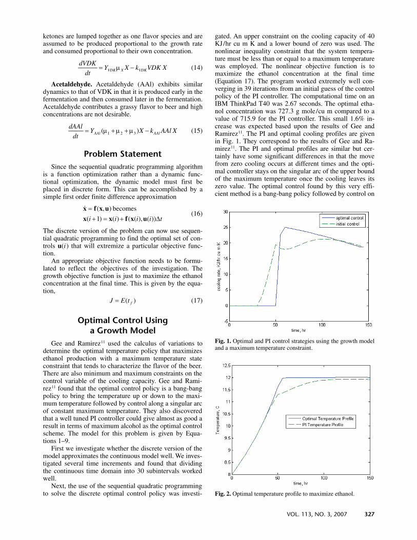
gated. An upper constraint on the cooling capacity of 40 KJ/hr cu m K and a lower bound of zero was used. The nonlinear inequality constraint that the system tempera-ture must be less than or equal to a maximum temperature was employed. The nonlinear objective function is to maximize the ethanol concentration at the final time (Equation 17). The program worked extremely well con-verging in 39 iterations from an initial guess of the control policy of the PI controller. The computational time on an IBM ThinkPad T40 was 2.67 seconds. The optimal etha-nol concentration was 727.3 g mole/cu m compared to a value of 715.9 for the PI controller. This small 1.6% in-crease was expected based upon the results of Gee and Ramirez11. The PI and optimal cooling profiles are given in Fig. 1. They correspond to the results of Gee and Ra-mirez11. The PI and optimal profiles are similar but cer-tainly have some significant differences in that the move from zero cooling occurs at different times and the opti-mal controller stays on the singular arc of the upper bound of the maximum temperature once the cooling leaves its zero value. The optimal control found by this very effi-cient method is a bang-bang policy followed by control on

Fig. 1. Optimal and PI control strategies using the growth model and a maximum temperature constraint.

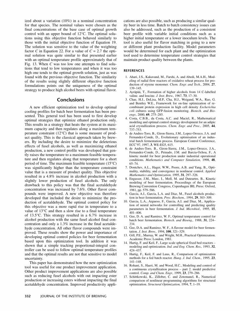
Fig. 2. Optimal temperature profile to maximize ethanol.

328 JOURNAL OF THE INSTITUTE OF BREWING

the singular arc. For this problem the optimal system is always on a constraint boundary using sequential quad-ratic programming of either the lower bound for the cool-ing or the nonlinear inequality constraint of a maximum system temperature.

The optimal temperature profile that maximizes etha-nol is given in Fig. 2 and shows that while the control is at its minimum value the temperature rises at its maximum rate, but that once the maximum temperature (12°C) was reached, it stayed on this singular arc.

Optimal Flavor Control The flavor components were then added to the mathe-

matical model. Gee and Ramirez12 report kinetic and yield parameters obtained from nonlinear curve fits for tem-peratures of 10.5°C, 12°C and 14.5°C. All the yield pa-rameters were averaged over these three temperatures but explicit temperature effects were included for the kinetic rate constants. Based upon Arrhenius plots, frequency fac-tors and activation energies were obtained through linear regression. All parameters were reasonable except for the

isoleucine correlation which showed a slight wrong direc-tion temperature effect. The isoleucine kinetic data were therefore averaged and an averaged rate constant was as-sumed to apply over the temperature range. The flavor ki-netic constants, as well as growth constants used in this study, are given in Table I.

The next goal was to include flavor aspects to maxi-mize an objective function that maximizes ethanol pro-duction, but does not increase the fusel alcohol concentra-tions over the previous case with a low maximum tem-perature constraint of 12°C. Keeping fusel alcohols low was deemed very important to the taste of the beer, as well as to the health of the consumer. A secondary con-cern was to increase the ester concentration if possible. A new objective function was proposed, which was to be maximized:

)]()()()([)( fffff tPtMBtIAtIBCtEJ +++−= (18)

Here the weighting factor C reflects the relative impor-tance of maximizing the final ethanol concentration to that of minimizing the sum of the fusel alcohol concentra-tions at the final time. For the base case, shown in Figs. 1 and 2, the final ethanol concentration was 727.3 gmole/cu m and the sum of the fusel alcohols was 1.507 gmole/cu m. For the two effects to be of equal importance the weighting factor C needs to be about 500.

Again the sequential quadratic programming approach was used but with a relaxation of the maximum tempera-ture inequality constraint, to be 15°C, which is the upper range value of temperature used to determine the kinetic parameters used in this study. Several different values of C were tried and a value of 900 showed a good compro-mise between the two effects in the objective function. The optimization from the control profile found from us-ing PI control around a set point of 12°C was started. The optimal results are given in Fig. 3 for the optimal cooling rate and Fig. 4 for the optimal temperature profile. These optimal conditions resulted in a final ethanol concentra-tion of 762.2 gmole/cu m which is a 4.8% improvement over the optimal growth value. The new optimal fusel alcohol concentrations sum to 1.505 which is slightly

Table I. List of terms.

Parameter Value Units

ln µG0 35.77 ln h–1 ln µM0 16.4 ln h–1 ln µN0 10.59 ln h–1 EG0 22.6 kcal /gmole EM0 11.3 kcal /gmole EN0 7.16 kcal /gmole ln KG0 –121.3 ln gmole /cu m ln KM0 –19.5 ln gmole /cu m ln KN0 –26.78 ln gmole /cu m EKG –68.6 kcal /gmole EKM –14.4 kcal /gmole EKN –19.9 kcal /gmole ln E′G0 23.33 ln gmole /cu m ln E′M0 55.61 ln gmole /cu m E′KG 10.2 kcal /gmole E′KM 26.3 kcal /gmole YXG 0.134 YXM 0.268 YXN 0.402 �HFG –91.2 kJ /gmole �HFM –226.3 kJ /gmole �HFN –361.3 kJ /gmole YLX 0.0832 YIX 0.0363 YVX 0.0273 KI 0.365 gmole /cu m ln KL0 10.14 ln gmole /cu m ln KV0 328 ln gmole /cu m EKL 5.95 kcal /gmole EKV 211.9 kcal /gmole �d 23.54 h YIB 0.203 YIA 0.557 YMB 0.472 YP 0.235 YEA 0.000992 YEC 0.000118 YIAc 0.0269 YVDK 0.000105 YAAl 0.01 ln k0

VDK 86.8 ln cu m/(h gmole) ln k0

AAl 10.4 ln cu m/(h gmole) EVDK 54.3 kcal /gmole EAAl 11.1 kcal /gmole Fig. 3. Optimal cooling rates for an optimal flavor objective.

VOL. 113, NO. 3, 2007 329

lower than the growth value of 1.507. Therefore additional alcohol was produced, while lowering the fusel alcohol concentration. This is a very important practical result. The problem took 136 iterations to converge and a com-putational time of 8.4 seconds on an IBM ThinkPad T40. If the value of C is too low, then the optimal growth model results are obtained of an initial period of no cooling fol-lowed by regulation at the maximum temperature. This does result in an increase in the fusel alcohol concentra-tion of 1.7%. If the value of C is too high then the fusel alcohol concentration is lowered at the expense of alcohol production (40% reduction) and the system temperature goes slowly down to very low values of 4.7°C.

The optimal flavor cooling policy shows that one starts cooling the system at the early times in order to keep a slow steady rate of rise of temperature and the fermenta-tion rate. At later times the cooling capacity is lowered, allowing the temperature to continue to slowly rise. At the very end of the cycle, the cooling rate is significantly in-creased approaching its maximum value.

The optimal temperature profile is given in Fig. 4. It shows a gentle almost linear rise, reaching the maximum near the end of the fermentation process. Significant cool-ing is now required to keep the temperature at or below its maximum value. These optimal conditions are signifi-cantly different from those based solely upon the growth model which shows a rapid rise in temperature and fer-mentation rate until the maximum temperature is reached and then regulation at that maximum temperature. The insights obtained here offer real promise for developing new control schemes that can increase alcohol production while minimizing fusel alcohol production.

In addition, these optimal conditions resulted in an in-crease in ester production from 0.2379 gmole/cu m to 0.2479 gmole/cu m. This is an increase of 3.8% in the production of flavor enhancing esters. It seems that in maximizing ethanol one also maximizes ester production.

Fig. 5 gives the optimal sugar consumption profile, Fig. 6 the optimal ethanol production profile, Fig. 7 the optimal amino acid consumption profile, Fig. 8 the opti-

Fig. 4. Optimal temperature profile using an optimal flavor ob-jective.

Fig. 5. Optimal sugar consumption using an optimal flavor ob-jective.

Fig. 6. Optimal ethanol production using an optimal flavor ob-jective.

Fig. 7. Optimal amino acid profiles using an optimal flavor ob-jective.

330 JOURNAL OF THE INSTITUTE OF BREWING

mal fusel alcohol profile, Fig. 9 the optimal ester profile, Fig. 10 the optimal VDK profile and Fig. 11 the optimal acetaldehyde profile.

The only draw back with this strategy was that the acetaldehyde final concentration actually increased by 7.6% and this could give the beer too grassy a flavor. However, the VDK concentration was reduced by 42.7%, which would tend to mitigate the acetaldehyde increase, although the VDK concentrations are much lower than that of acetaldehyde (see Figs. 10 and 11). In order to re-duce the final acetaldehyde concentration a new objective function was used:

)(

)]()()()([)(

2

1

f

fffff

tAAlC

tPtMBtIAtIBCtEJ

−

+++−=

(19)

Using values of C1 of 810 and C2 of 610 the optimal cool-ing capacity shown in Fig. 12 and the optimal system tem-perature profile of Fig. 13 was obtained. The problem converged in 54 iterations with a computational time of

10.1 seconds. The optimal results have an increase in the final ethanol concentration of 6.2%, an increase in the final ester concentration of 4.6%, a fusel alcohol concen-tration that stays the same, a decrease in the final VDK concentration of 26.7% and a slight increase in the final acetaldehyde concentration of 1.27%. The optimal tem-perature policy shows a steady initial rise in temperature near its maximum rate, using some cooling to modify these early rates of change. Once a temperature of 13°C was reached, the cooling increased in order to raise the temperature gradually to around 13.5°C. Again the opti-mal control approach has been able to develop a new op-erational strategy that is a significant improvement over the conventional optimal growth policy.

The values of C1 and C2 can significantly change the results. When they are low, the optimal growth policy is obtained which results in excess production of fusel alco-hols (1.7%) and acetaldehyde (2.3%). When they are too large, the system is excessively cooled resulting in a 40% reduction in ethanol production.

Fig. 8. Optimal fusel alcohol profiles using an optimal flavor ob-jective.

Fig. 10. Optimal VDK profile using an optimal flavor objective.Fig. 11. Optimal acetaldehyde profile using an optimal flavor ob-jective.

Fig. 9. Optimal ester profiles using an optimal flavor objective.

VOL. 113, NO. 3, 2007 331

Implementation The regulation of the system using a tracking PI con-

troller about the optimal temperature profile was investi-gated. A velocity mode for the PI algorithm was used,

)( )1()()()1()( −−Δ+Δ+−= keketKPketKIkuku (20)

Here k denotes the time index, �t the time interval, KI the integral gain and KP the proportional gain. The tracking error, e(k) is given by

)()()( optimal kTkTke −= (21)

where Toptimal (k) is the optimal value of the temperature at any time t(k).

Fig. 14 shows that a tracking regulator can follow the optimal temperature profile well with KP = 40 and KI = 5. The final ethanol concentration was within 0.3% of the optimal value, the fusel alcohol concentration within 0.1% and the acetaldehyde concentration within 0.1% of the optimal value. The esters and VDK concentrations were

the same as with the optimal conditions. These results showed that the optimal flavor results can easily be imple-mented with simple feedback controllers.

The effect of model uncertainty was also investigated. One of the least well known parameters is that of the acet-aldehyde consumption rate constant kAAl In order to in-vestigate this, the natural log of the frequency factor ln k0

AAl was increased by 10%. This resulted in a significantly lower final concentration of acetaldehyde of 0.218 gmole/ cu m. The optimal temperature profile for this case was essentially that of Fig. 13 so that regulating about that profile still resulted in beer with optimal flavor. The malt-ose activation energy was also lowered, from 11.3 kcal / gmole to 10.93 kcal /gmole, which consumes significantly more maltose than the base case. This raised the optimal growth final ethanol concentration to 967.7 gmole/cu m. The optimal flavor temperature profile was however es-sentially that of Fig. 13 and regulating about that profile gives essentially the same result as an optimal profile based upon Equation 19. This shows that the optimal tem-perature profile of Fig. 13 was quite insensitive to model uncertainty and could be used for beers that approximately follow the model parameters of this study. The optimal temperature profile seems to more a function of the model structure than specific model parameters.

As part of the investigation of the robustness of the op-timal temperature profile, a slightly different optimization objective function was considered.

2

nom

2

nom

2

nom

2

nom

2

nom

2

nom

)(1.0

)(

)(1.0

)(

)(1.0

)(

)(1.0

)(

)(1.0

)(

)(1.0

)(

⎟⎟⎠

⎞⎜⎜⎝

⎛⎟⎟⎠

⎞⎜⎜⎝

⎛⎟⎟⎠

⎞⎜⎜⎝

⎛

⎟⎟⎠

⎞⎜⎜⎝

⎛⎟⎟⎠

⎞⎜⎜⎝

⎛+⎟

⎟⎠

⎞⎜⎜⎝

⎛

+++

+−=

f

f

f

f

f

f

f

f

f

f

f

f

tAAl

tAAl

tP

tP

tMB

tMB

tIA

tIA

tIB

tIB

tE

tECJ

(22)

Again, the goal was to try to maximize the final ethanol concentration while minimizing the fusel alcohol and acet-aldehyde concentration. Each concentration was normal-

Fig. 13. Optimal temperature policy including acetaldehyde mini-mization.

Fig. 14. Temperature regulation about the optimal temperatureprofile.

Fig. 12. Optimal cooling including acetaldehyde minimization.

332 JOURNAL OF THE INSTITUTE OF BREWING

ized about a variation (10%) in a nominal concentration for that species. The nominal values were chosen as the final concentrations of the base case of optimal growth control with an upper bound of 12°C. The optimal solu-tions using this objective function behaved similarly to those with the initial objective function of Equation 19. The solution was sensitive to the value of the weighting factor C in Equation 22. For a value of C = 2.7 the opti-mal solution was quite similar to that presented earlier with an optimal temperature profile approximately that of Fig. 13. When C was too low one attempts to find solu-tions that tend to low temperatures and when it was too high one tends to the optimal growth solution, just as was found with the previous objective function. The similarity of the results using slightly different objective function formulations points out the uniqueness of the optimal strategy to produce high alcohol beers with optimal flavor.

Conclusions A new efficient optimization tool to develop optimal

cooling profiles for batch beer fermentation has been pre-sented. This general tool has been used to first develop optimal strategies that optimize ethanol production only. This results in a strategy that heats the system at its maxi-mum capacity and then regulates along a maximum tem-perature constraint (12°C) that is some measure of prod-uct quality. This is the classical approach taken by brew-ers. By including the desire to minimize the deleterious effects of fusel alcohols, as well as maximizing ethanol production, a new control profile was developed that gen-tly raises the temperature to a maximum feasible tempera-ture and then regulates along that temperature for a short period of time. The maximum feasible temperature (15°C) was significantly higher than the temperature constraint value that is a measure of product quality. This objective resulted in a 4.8% increase in alcohol production with a slightly lower production of fusel alcohols. The only drawback to this policy was that the final acetaldehyde concentration was increased by 7.6%. Other flavor com-pounds were improved. A new objective was therefore developed that included the desire to minimize the pro-duction of acetaldehyde. The optimal control policy for this objective was a more rapid rise in temperature to a value of 13°C and then a slow rise to a final temperature of 13.5°C. This strategy resulted in a 6.7% increase in alcohol production with the same fusel alcohol final con-centration and only a 1.3% increase in the final acetalde-hyde concentration. All other flavor compounds were im-proved. These results show the power and importance of developing optimal control policies for beer fermentation based upon this optimization tool. In addition it was shown that a simple tracking proportional-integral con-troller can be used to follow optimal temperature profiles and that the optimal results are not that sensitive to model uncertainty.

This paper has demonstrated how the new optimization tool was useful for one product improvement application. Other product improvement applications are also possible such as reducing fusel alcohols with out impacting ester production or increasing esters without impacting the final acetaldehyde concentration. Improved productivity appli-

cations are also possible, such as producing a similar qual-ity beer in less time. Batch to batch consistency issues can also be addressed, such as the production of a consistent beer profile with variable initial conditions such as a higher initial temperature or a lower inoculum levels. The tool is also useful for flavor matching in going to a new or different plant production facility. Model parameters would be determined for each plant and the optimization tool used to determine temperature control strategies that maintain product quality between the plants.

REFERENCES

1. Ahari, J.S., Kakavand, M., Farshi, A. and Abedi, M.A.H., Mod-eling of radial flow reactors of oxidative reheat process for pro-duction of styrene monomer. Chem. Engr. and Tech., 2004, 27, 139–145.

2. Ayräpää, T., Formation of higher alcohols from 14 C-labelled valine. and leucine. J. Inst. Brew., 1967, 73, 17–30.

3. Chae, H.J., DeLisa, M.P., Cha, H.J., Weigand, W.A., Rao, G. and Bentley W.E., Framework for on-line optimization of re-combinant protein expression in high cell density Escherichia coli cultures using GFP-fusion monitoring. Biotech. and Bio-engr., 2000, 69, 275–285.

4. Costa, C.B.B., da Costa, A.C. and Maciel, R., Mathematical modeling and optimal control strategy development for an adipic acid crystallization process. Chem. Engr. and Proc., 2005, 44, 737–753.

5. de Andres-Toro, B., Giron-Sierra, J.M., Lopez-Orozco, J.A. and Fernandez-Conde, D., Evolutionary optimisation of an indus-trial batch fermentation process. European Control Conference, ECC’97, 1997, 3, WE-EG5, 615.

6. de Andres-Toro, B., Giron-Sierra, J.M., Lopez-Orozco, J.A., Fernandez-Conde, D., Peinado, J.M. and Barcia-Ochoa, F., A kinetic model for beer production under industrial operational conditions. Mathematics and Computer Simulation, 1998, 48, 65–74.

7. Dontchev, A.L., Hager, W.W., Poore, A.B. and Yang, B., Opti-mality, stability, and convergence in nonlinear control. Applied Mathematics and Optimization, 1995, 31, 297–326.

8. Engasser, J.M., Marc, I., Moll, M. and Duteurtre, B., Kinetic modeling of beer fermentation. Proceedings of the European Brewing Convention Congress, Copenhagen IRL Press: Oxford, 1981, pp. 579–586.

9. Garcia, A.I., Garcia, L.A. and Diaz, M., Fusel alcohols produc-tion in beer fermentation. Proc. Biochem., 1994, 29, 303–309.

10. Garcia, L.A., Argueso, F., Garcia, A.I. and Diaz, M., Applica-tion of neural networks for controlling and predicting quality parameters in beer fermentation. J. Ind. Microbiol., 1995, 15, 401–406.

11. Gee, D. A. and Ramirez, W. F., Optimal temperature control for batch beer fermentation. Biotech. and Bioeng., 1988, 31, 224–234.

12. Gee, D.A. and Ramirez, W. F., A flavour model for beer fermen-tation. J. Inst. Brew., 1994, 100, 321–329.

13. Gill, P.E., Murray, W. and Wright, M.H., Practical Optimization. Academic Press: London, 1981.

14. Hartig, F. and Keil, F., Large scale spherical fixed bed reactors – modeling and optimization. Ind. and Eng. Chem. Res., 1993, 32, 424–437.

15. Hartig, F., Keil, F. and Luus, R., Comparison of optimization methods for a fed batch reactor. Hung. J. Ind. Chem., 1995, 23, 141–148.

16. Rohani, S., Haeri, M. and Wood, H.C., Modeling and control of a continuous crystallization process – part 2. model predictive control. Comp. and Chem. Engr., 1999, 23, 279–286.

17. Schittkowski, K., Zillober, C. and Zotemanel, R., Numerical comparison of nonlinear programming algorithms for structural optimization. Structural Optimization, 1994, 7, 1–19.

VOL. 113, NO. 3, 2007 333

18. Shukla, P.K. and Pushpavanam, S., Optimisation of biochemical reactors – an analysis of different approximations of fed batch operation. Chem. Eng. Sci., 1998, 53, 341–352.

19. Tada, K., Kishimoto, M., Omasa, T., Katakura, Y. and Suga, K.I., Constrained optimization of L-lysine production based on metabolic flux using a mathematical programming method. J. Biosci. and Bioengr., 2001, 91, 344–351.

20. Takeda, M. and Ray, W.H., Optimal grade transition strategies for multistage polyolefin reactors. AIChE J., 1999, 45, 1776–1793.

21. Tian, Y., Zhang, J. and Morris, J., Optimal control of a batch emulsion copolymerisation reactor based on recurrent neural network models. Chem. Eng. Proc., 2002, 41, 531–538.

22. Titica, M., Landaud, S., Trelea, I.C., Latrille, E., Corrieu, G. and Cheruy, A., Modeling of the kinetics of higher alcohol and ester production based on CO2 emission with a view to control of

beer flavor by temperature and top pressure. J. Am. Soc. Brew-ing Chemists, 2000, 58, 167–174.

23. Trelea, I.C., Titica, M., Landaud, S., Latrille, E., Corrieu, G. and Cheruy, A., Predictive modelling of brewing fermentation: from knowledge-based to black-box models. Math. and Comp. in Sim., 2001 56, 405–424.

24. Trelea, I.C., Titica, M. and Corrieu, G., Dynamic optimisation of the aroma production in brewing fermentation. J. Proc. Con-trol, 2004, 14, 1–16.

25. Wang, F.S. and Shyu, C.H., Optimal feed policy for fed batch fermentation of ethanol production by Zymomonus mobilis. Bio-proc. Engr., 1997, 17, 63–68.

(Manuscript accepted for publication September 2007)