
Optimal Beamforming 1 Introductionrsadve/Notes/BeamForming.pdf · We begin by developing the theory...
21
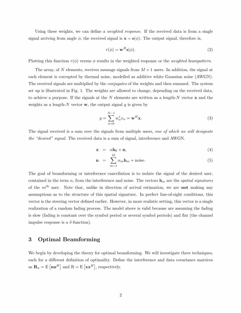
Optimal Beamforming 1 Introduction In the previous section we looked at how fixed beamforming yields significant gains in communi- cation system performance. In that case the beamforming was fixed in the sense that the weights that multiplied the signals at each element were fixed (they did not depend on the received data). We now allow these weights to change or adapt, depending on the received data to achieve a certain goal. In particular, we will try to adapt these weights to suppress interference. The interference arises due to the fact that the antenna might be serving multiple users. Output Signal Σ w 0 * w 1 * w N-1 * Figure 1: A general beamforming system. 2 Array Weights and the Weighted Response Figure 1 illustrates the receive beamforming concept. The signal from each element (x n ) is multi- plied with a weight w * n , where the superscript * represents the complex conjugate. Note that the conjugate of the weight multiplies the signal, not the weight itself. The weighted signals are added together to form the output signal. The output signal r is therefore given by r = N -1 n=0 w * n x n , = w H x, (1) where w represents the length N vector of weights, x represents the length N vector of received signals and the superscript H represents the Hermitian of a vector (the conjugate transpose), i.e., w H = w * 0 ,w * 1 , ... w * N -2 ,w * N -1 = w T * . 1
Transcript of Optimal Beamforming 1 Introductionrsadve/Notes/BeamForming.pdf · We begin by developing the theory...

Optimal Beamforming
1 Introduction
In the previous section we looked at how fixed beamforming yields significant gains in communi-
cation system performance. In that case the beamforming was fixed in the sense that the weights
that multiplied the signals at each element were fixed (they did not depend on the received data).
We now allow these weights to change or adapt, depending on the received data to achieve a certain
goal. In particular, we will try to adapt these weights to suppress interference. The interference
arises due to the fact that the antenna might be serving multiple users.
Output Signal
Σ
w0*
w1*
wN-1
*
Figure 1: A general beamforming system.
2 Array Weights and the Weighted Response
Figure 1 illustrates the receive beamforming concept. The signal from each element (xn) is multi-
plied with a weight w∗n, where the superscript ∗ represents the complex conjugate. Note that the
conjugate of the weight multiplies the signal, not the weight itself. The weighted signals are added
together to form the output signal. The output signal r is therefore given by
r =N−1∑
n=0
w∗
nxn,
= wHx, (1)
where w represents the length N vector of weights, x represents the length N vector of received
signals and the superscript H represents the Hermitian of a vector (the conjugate transpose), i.e.,
wH =[
w∗0, w∗
1, . . . w∗
N−2, w∗
N−1
]
=[
wT]∗
.
1
Using these weights, we can define a weighted response. If the received data is from a single
signal arriving from angle φ, the received signal is x = s(φ). The output signal, therefore is,
r(φ) = wHs(φ). (2)
Plotting this function r(φ) versus φ results in the weighted response or the weighted beampattern.
The array, of N elements, receives message signals from M + 1 users. In addition, the signal at
each element is corrupted by thermal noise, modelled as additive white Gaussian noise (AWGN).
The received signals are multiplied by the conjugates of the weights and then summed. The system
set up is illustrated in Fig. 1. The weights are allowed to change, depending on the received data,
to achieve a purpose. If the signals at the N elements are written as a length-N vector x and the
weights as a length-N vector w, the output signal y is given by
y =N−1∑
n=0
w∗
nxn = wHx. (3)
The signal received is a sum over the signals from multiple users, one of which we will designate
the “desired” signal. The received data is a sum of signal, interference and AWGN.
x = αh0 + n, (4)
n =M∑
m=1
αmhm + noise. (5)
The goal of beamforming or interference cancellation is to isolate the signal of the desired user,
contained in the term α, from the interference and noise. The vectors hm are the spatial signatures
of the mth user. Note that, unlike in direction of arrival estimation, we are not making any
assumptions as to the structure of this spatial signature. In perfect line-of-sight conditions, this
vector is the steering vector defined earlier. However, in more realistic setting, this vector is a single
realization of a random fading process. The model above is valid because are assuming the fading
is slow (fading is constant over the symbol period or several symbol periods) and flat (the channel
impulse response is a δ-function).
3 Optimal Beamforming
We begin by developing the theory for optimal beamforming. We will investigate three techniques,
each for a different definition of optimality. Define the interference and data covariance matrices
as Rn = E[
nnH]
and R = E[
xxH]
, respectively.
2

3.1 Minimum Mean Squared Error
The minimum mean squared error (MMSE) algorithm minimizes the error with respect to a reference
signal d(t). In this model, the desired user is assumed to transmit this reference signal, i.e., α =
βd(t), where β is the signal amplitude and d(t) is known to the receiving base station. The output
y(t) is required to track this reference signal. The MMSE finds the weights w that minimize the
average power in the error signal, the difference between the reference signal and the output signal
obtained using Eqn. (3)
wMMSE = arg minw
E{
|e(t)|2}
, (6)
where
E{
|e(t)|2}
= E{
∣
∣wHx(t) − d(t)∣
∣
2}
,
= E{
wHxxHw − wHxd∗ − xHwd+ dd∗}
,
= wHRw − wHrxd − rHxdw + dd∗, (7)
where
rxd = E {xd∗} . (8)
To find the minimum of this functional, we take its derivative with respect to wH (we have seen
before that we can treat w and wH as independent variables).
∂E{
|e(t)|2}
∂wH= Rw − rxd = 0,
⇒ wMMSE = R−1rxd. (9)
This solution is also commonly known as the Wiener filter.
We emphasize that the MMSE technique minimizes the error with respect to a reference signal.
This technique, therefore, does not require knowledge of the spatial signature h0, but does require
knowledge of the transmitted signal. This is an example of a training based scheme: the reference
signal acts to train the beamformer weights.
3.2 Minimum Output Energy
The minimum output energy (MOE) beamformer defines a different optimality criterion: we min-
imize the total output energy while simultaneously keeping the gain of the array on the desired
signal fixed. Because the gain on the signal is fixed, any reduction in the output energy is obtained
3
by suppressing interference. Mathematically, this can be written as
wMOE = arg minw
E{
|y|2}
, wHh0 = c,
≡ arg minw
E{
∣
∣wHx∣
∣
2}
, wHh0 = c. (10)
This final minimization can be solved using the method of Lagrange multipliers, finding minw [L(w;λ)],
where
L(w;λ) = E{
∣
∣wHx∣
∣
2}
+ λ[
wHh0 − c]
,
= E{
wHxxHw}
+ λ[
wHh0 − c]
,
= wHRw + λ(
wHh0 − c)
, (11)
⇒∂L
∂wH= Rw + λh0
⇒ wMOE = −λR−1h0 (12)
Using the constraint on the weight vector, the Lagrange parameter λ can be easily obtained by
solving the gain constraint, setting the final weights to be
wMOE = cR−1h0
hH0 R−1h0
. (13)
Setting the arbitrary constant c = 1 gives us the minimum variance distortionless response (MVDR),
so called because the output signal y has minimum variance (energy) and the desired signal is not
distorted (the gain on the signal direction is unity).
Note the MOE technique does not require a reference signal. This is an example of a blind
scheme. The scheme, on the other hand, does require knowledge of the spatial signature h0. The
technique “trains” on this knowledge.
3.3 Maximum Output Signal to Interference Plus Noise Ratio - Max SINR
Given a weight vector w, the output signal y = wHx = αwHh0 + wHn, where n contains both
interference and noise terms. Therefore, the output signal to interference plus noise ratio (SINR)
is given by
SINR = E{
|α|2}
∣
∣wHh0
∣
∣
2
E{
|wHn|2} = A2
∣
∣wHh0
∣
∣
2
E{
|wHn|2} , (14)
4

where A2 = E{
|α|2}
is the average signal power. Another (reasonable) optimality criterion is to
maximize this output SINR with respect to the output weights.
wMax SINR = arg maxw
{SINR} . (15)
We begin by recognizing that multiplying the weights by a constant does not change the output
SINR. Therefore, since the spatial signature h0 is fixed, we can choose a set of weights such that
wHh0 = c. The maximization of SINR is then equivalent to minimizing the interference power, i.e.
wMax SINR = minw
E{
∣
∣wHn∣
∣
2}
= wHRnw, wHh0 = c. (16)
We again have a case of applying Lagrange multipliers, as in Section 3.2, with R replaced with Rn.
Therefore,
w = cR−1n h0
hH0 R−1n h0
. (17)
3.4 Equivalence of the Optimal Weights
We have derived three different weight vectors using three different optimality criteria. Is there a
“best” amongst these three? No! We now show that, in theory, all three schemes are equivalent. We
begin by demonstrating the equivalence of the MOE and Max SINR criteria. Using the definitions
of the correlation matrices R and Rn,
R = Rn +A2h0hH0 (18)
Using the Matrix Inversion Lemma1
R−1 =[
Rn +A2h0 hH0]−1
,
⇒ R−1 = R−1n −
R−1n h0 hH0 R−1
n
hH0 R−1n h0 +A−2
, (19)
⇒ R−1h0 = R−1n h0 −
R−1n h0 hH0 R−1
n h0
hH0 R−1n h0 +A−2
,
= R−1n h0 −
(
hH0 R−1n h0
)
R−1n h0
hH0 R−1n h0 +A−2
,
=
(
A−2
hH0 R−1n h0 +A−2
)
R−1n h0,
= cR−1n h0, (20)
1[A + BCD]−1 = A−1
− A−1
B[
DA−1
B + C−1
]
−1
DA−1
5

i.e., the adaptive weights obtained using the MOE and Max SINR criteria are proportional to each
other. Since multiplicative constants in the adaptive weights do not matter, these two techniques
are therefore equivalent.
To show that the MMSE weights (Wiener filter) and the MOE weights are equivalent, we start
with the definition of rxd,
rxd = E {xd∗(t)} ,
= E {[αh0 + n] d∗(t)} . (21)
Note that the term α = βd(t), where β is some amplitude term and d(t) is the reference signal.
Therefore,
rxd = β|d|2h0 + E {n} d∗(t)
= β|d|2h0
∝ h0
⇒ wMMSE ∝ wMOE (22)
i.e., the MMSE weights and the MOE weights are also equivalent. Therefore, theoretically, all three
approaches yield the same weights starting from different criteria for optimality. We will see that
these criteria are very different in practice.
3.5 Suppression of Interference
We can use the matrix inversion lemma to determine the response of the optimal beamformer to a
particular interference source. Since all three beamformers are equivalent, we can choose any one of
the three. We choose the MOE. Within a constant, the optimal weights are given by w = R−1h0.
Denote as Q the interference correlation matrix without the particular interference source (assumed
to have amplitude αi, with E{
|αi|2}
= Ai, and spatial signature hi. In this case,
R = Q + E{
|α|2}
hihHi
= Q +AihihHi
⇒ R−1 = Q−1 −A2iQ
−1hihHi Q−1
1 +A2ih
Hi Q−1hi
6

The gain of the beamformer (with the interference) on the interfering source is given by wHhi.
Using the definition of the weights,
wHhi = hH0 R−1hi
= h0Q−1hi −
A2i
[
hH0 Q−1hi] [
hHi Q−1hi]
1 +A2ih
Hi Q−1hi
=hH0 Q−1hi
1 +A2ih
Hi Q−1hi
(23)
The numerator in the final equation is the response of the optimal beamformer on the interference
if the interferer were not present. The denominator represents the amount by which this response
is reduced due to the presence of the interferer. Note that the amount by which the gain is reduced
is dependent on the power of the interference (corresponding to A2i ). The stronger the interference
source, the greater is it suppressed. An optimal beamformer may “ignore” a weak interfering source.
Figure 2 illustrates the performance of the optimal beamformer. This example uses line of sight
conditions, which allows us to use “beampatterns”. However, it must be emphasized that this is
for convenience only. In line of sight conditions, the direction of arrival, φ, determines the spatial
signature to be the steering vector, s(φ), as developed earlier in this course. In the first case, there
are two interferers at angles φ = 30o, 150o and in the other, there two interferers at φ = 40o, 150o.
The desired signal is at φ = 0. Note how the null moves over from 30o to 40o. It is important to
realize that the optimal beamformer creates these nulls (suppresses the interfering sources) without
a-priori knowledge as to the location of the interference sources.
If there are more interfering sources than elements, all sources cannot be nulled (a N element
array can only null N − 1 interfering signals). In this case, the beamformer sets the weights to
minimize the overall output interference power. Figure 3 illustrates this situation. The solid line is
the case of seven equally strong interfering sources received by a five element antenna array (N = 5).
Note that the array, apparently, forms only four nulls. These nulls do not correspond directly to the
locations of the interference as it is the overall interference that is being minimized. The dashed line
plots the beampattern in the case that one of the seven interfering sources, arriving from φ = 40o,
is extremely strong. Note that the beamformer automatically moves a null in direction of this
strong interferer (to the detriment of the suppression of the other interfering sources - again, it is
the overall interference power that is minimized).
3.6 Relation of Beampattern and Noise
In this section we focus on the impact the weights have on the noise component. Again, the term
”beampattern” has a connotation that beamforming is for line of sight conditions only. In point
of fact, a beampattern can always be defined. However, in multipath fading channels, the desired
7

20 40 60 80 100 120 140 160 180
−60
−50
−40
−30
−20
−10
0
φ
dB
φi = 30, 150
φi = 40,150
5 element array
Figure 2: Illustration of nulling using the optimal beamformer.
20 40 60 80 100 120 140 160 180
−70
−60
−50
−40
−30
−20
−10
0
φ
dB
7 equally strong signalsVery strong signal at 40o
5 element array
Figure 3: Nulling with number of interferers greater than number of elements.
8

signal does not arrive from a single direction. We assume that the noise at each element is white,
independent, zero mean and Gaussian, with noise power σ2, i.e., E[
nnH]
= σ2I. Here, in an abuse
of notation we use n to represent noise (which was noise and interference in the earlier sections).
The noise component in the output signal is wHn, i.e. the noise power in the output (σ2o) is
given by
σ2o = E
[
∣
∣wHn∣
∣
2]
= E
∣
∣
∣
∣
∣
N−1∑
i=0
w∗
i ni
∣
∣
∣
∣
∣
2
, (24)
= σ2
N−1∑
i=0
|wi|2 . (25)
The noise is, therefore, enhanced by the “total energy” in the weights. Now, consider the
adapted beam pattern. In direction φ the gain of the array due to the weights is given by
wHs(φ),where s(φ) is the steering vector associated with direction φ. In fact, due to the structure
of the steering vector, setting ψ = kd cosφ,
G(ψ) =N−1∑
n=0
wnejnψ, (26)
i.e., in ψ space, the beam pattern is the DFT of the weights. Therefore, due to Parseval’s theorem,
N−1∑
i=0
|wi|2 =
∫ 2π
0
|G(ψ)|2 dψ, (27)
i.e., the enhancement of the noise power is the same as total area under the beampattern. Clearly,
if the adapted pattern had high sidelobes, the noise would be enhanced. Therefore, in trying to
suppress interference, the beamforming algorithm (MOE/MMSE/Max SINR) also attempts to keep
sidelobes low, thereby maximizing the overall SINR.
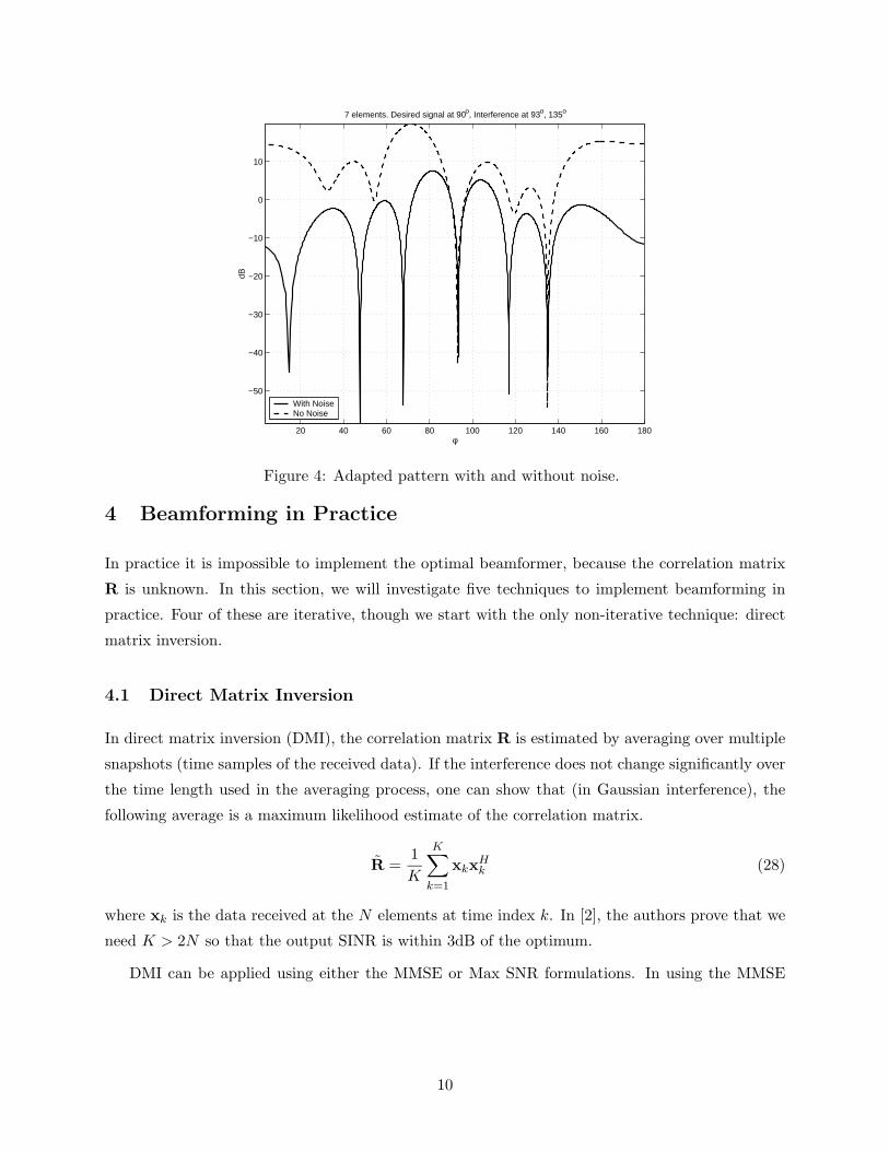
Figure 4 plots the adapted beampattern in the case of signals with noise and signals without
noise. Clearly, is noise were absent the minimum interference power is achieved by a set of weights
that result in high sidelobes. If these weights were used in a real system, they would minimize
interference power, but enhance the noise power. The solid line plots the adapted beam pattern
with exactly the same signal and interference data, but now noise is also added in. Note both plots
pas through 0dB at the direction of the desired signal (0o). Clearly to minimize SINR (not SIR),
the sidelobes must come down.
This issue is of relevance when trying to use algorithms such as zero-forcing in the spatial case.
Zero-forcing is a technique that focuses on the interference only and is best known when imple-
menting transmit beamforming (as opposed to the receive beamforming we have been doing) [1]. It
is well known that zero-forcing enhances noise. This is because in attempting to cancel interference
only, it lets the sidelobes rise, resulting in higher noise power.
9
20 40 60 80 100 120 140 160 180
−50
−40
−30
−20
−10
0
10
φ
dB
7 elements. Desired signal at 90o, Interference at 93o, 135o
With NoiseNo Noise
Figure 4: Adapted pattern with and without noise.
4 Beamforming in Practice
In practice it is impossible to implement the optimal beamformer, because the correlation matrix
R is unknown. In this section, we will investigate five techniques to implement beamforming in
practice. Four of these are iterative, though we start with the only non-iterative technique: direct
matrix inversion.
4.1 Direct Matrix Inversion
In direct matrix inversion (DMI), the correlation matrix R is estimated by averaging over multiple
snapshots (time samples of the received data). If the interference does not change significantly over
the time length used in the averaging process, one can show that (in Gaussian interference), the
following average is a maximum likelihood estimate of the correlation matrix.
R =1
K
K∑
k=1
xkxHk (28)
where xk is the data received at the N elements at time index k. In [2], the authors prove that we
need K > 2N so that the output SINR is within 3dB of the optimum.
DMI can be applied using either the MMSE or Max SNR formulations. In using the MMSE
10

Figure 5: PDF of the output SINR when the signal is and is not present in the training data whenusing the blind MOE technique
criterion, the cross correlation vector rxd is estimated by
rxd =1
K
K∑
k=1
d∗kxk, (29)
wMMSE = R−1rxd (30)
i.e., using DMI in this fashion requires a sequence of K known transmitted symbols, also known as
a training sequence. This is our first example of a training based beamforming procedure. On the
other hand, a blind procedure does not require a training sequence. DMI may also be applied in
this fashion using the MOE criterion.
wMOE = R−1h0. (31)
The problem with this procedure is that, as shown in [3], the data used to estimate the correla-
tion matrix xk must be signal-free, i.e., it is only possible to use the Max SINR criterion. Figure 5
plots the output pdf normalized output SINR (normalized with respect to the theoretical optimal).
The two plots are for K = 200. Clearly, in both cases, when the signal is present in the training
data, the pdf of the output SINR is significantly to the left (the mean is much lower) than when
the signal is absent. The physical interpretation appears to be that the MOE process assumes all
the signals in the training data is interference. So, the MOE approach tries to place a null and a
maximum simultaneously in the direction of the desired signal.
This problem is well established in radar systems, where a guard range is placed to eliminate
any of the desired signal. In a communication system, on the other hand, this would imply that
the desired user must stay silent in the training phase. Of course, if the desired signal is silent, this
is equivalent to the Max SINR criterion. This is in direct contrast to the MMSE criterion where
the user must transmit a known signal. It must be emphasized that this problem only occurs when
the correlation matrix is estimated. We have already shown that when the true matrix is known,
the MMSE and Max SNR techniques are equivalent.
11

20 40 60 80 100 120 140 160 180
−65
−60
−55
−50
−45
−40
−35
−30
−25
−20
−15
Azimuth Angle φ
dB
DMI using MMSEDMI using Max SNR
Figure 6: Adapted beampattern using the MMSE and Max SNR techniques.
Figure 6 illustrates the problem of having the desired signal in the training data. The example
uses an 11-element array (N = 11) with five signals at φ = 90o, 61o, 69.5o, 110o, 130o, . The signal
at φ = 90o is the desired signal while the other signals are interference. Using the DMI technique
with the MMSE as in Eqn. (30) the adapted beampattern using the MMSE version of DMI clearly
shows nulls in direction of the interference. However, when using the MOE version of DMI (using
Eqn. (31)) the beampattern retains the nulls, but the overall pattern is significantly corrupted.
We know that high sidelobes implies worse SNR, i.e., the MOE approach has severely degraded
performance if the desired signal is present in the training data.
We next look at iterative techniques for beamforming in practice. Before we explore these
techniques we need to understand iterative techniques in general. We begin the discussion with
the Steepest Descent algorithm which is an iterative technique to find the minimum of a functional
when the functional is known exactly.
4.2 Steepest Descent
The steepest descent technique is an iterative process to find the minimum of a functional, in our
case, a functional of the weight vector w. We want to find the solution to a matrix equation
Rw = rxd, however the functional being minimized is f(w) = E[
∣
∣wHx − d∣
∣
2]
. This functional
can be thought of being a function of N variables, [w0, w1, . . . , wN−1].
Assume that at the k-th iteration we have an estimate of the weights wk. We look to find a
better estimate by modifying wk in the form wk + ∆w. We know any function increases fastest
12

in direction of its gradient, and so it decreases fastest in the opposite direction. The steepest
descent therefore finds the correction factor ∆w in the direction opposite to that of the gradient,
i.e. ∆w = −µ▽f , µ > 0. Here, µ is called the step-size. Therefore, at the (k + 1)-th step,
wk+1 = w + ∆w,
= w − µ▽f, (32)
f(w) = E[
∣
∣wHx − d∣
∣
2]
,
= wHRw − wHrxd − rHxdw + |d|2 (33)
⇒ ▽f(w) = 2∂f
∂wH= Rw − rxd. (34)
This results in the relationship
wk+1 = wk − µ▽f
= wk + µ (rxd − Rwk) . (35)
Note that, other than a factor of the stepsize µ, the change in the weight vector is determined by
the error term, at the kth step, in the matrix equation Rw = rxd.
4.2.1 The range of µ
An immediate question that arises is how to choose µ. Conceivably, a large value of µ would
make the solution converge faster. However, as in any iteration process, an extremely large step
size could make the iterations unstable. We, therefore, need to determine the range of µ that
guarantees convergence. The iterative process must converge to the solution of the above matrix
equation
Rw = rxd.
Let wo (o for optimal, do not confuse with k = 0, the initial guess) be the solution to this equation.
The error at the k-th step is ek = wk − wo.
Subtracting the optimal solution from both sides of Eqn. (35), we get
wk+1 − wo = wk − wo + µ (rxd − Rwk)
⇒ ek+1 = ek + µ (rxd − Rwk) . (36)
However, since rxd = Rwo,
ek+1 = ek + µ (Rwo − Rwk) ,
ek+1 = ek − µRek,
= (I − µR) ek (37)
13

Writing the correlation matrix R in its eigenvalue decomposition, R = QΛQH , where QHQ =
QQH = I, we are write the final equation as
ek+1 = Q [I − µΛ]QHek, (38)
⇒ QHek+1 = [I − µΛ]QHek. (39)
Let ek = QHek. Therefore,
ek+1 = [I − µΛ] ek. (40)
Since Λ is a diagonal matrix of the eigenvalues, this equation represents an uncoupled system of
equations and each individual term can be written separately. The n-th term can be written as
ek+1,n = (1 − µλn)ek,n,
= (1 − µλn)k+1e0,n. (41)
Therefore, if the solution is to converge, the exponent term must tend to zero, i.e.
|1 − µλn| < 1,
⇒ −1 < 1 − µλn < 1,
⇒ 0 < µ <2
λn, (42)
Since this inequality must be true for all values of n, 0 ≤ n ≤ N − 1, the inequality that µ must
satisfy is
0 ≤ µ ≤2
λmax
. (43)
Therefore, the highest possible value of the step size is set by the largest eigenvalue of the correlation
matrix.
Finally, there are a few points about the steepest descent approach that must be emphasized:
• This form of eigendecomposition based analysis is common in iterative techniques based on
a matrix.
• The steepest descent algorithm is not adaptive. So far, all we have seen is an iterative method
to solve for the optimal weights.
• Choosing a ”good” value of µ is essential for the algorithm to converge without numerical
instabilities.
14
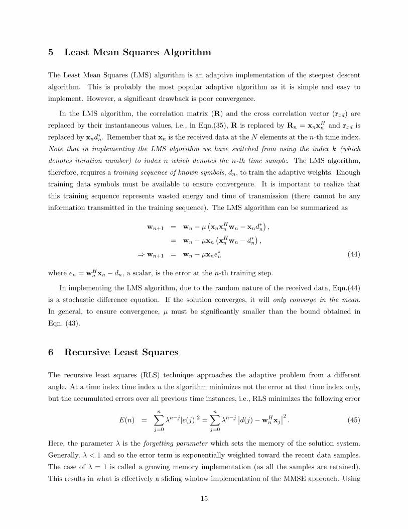
5 Least Mean Squares Algorithm
The Least Mean Squares (LMS) algorithm is an adaptive implementation of the steepest descent
algorithm. This is probably the most popular adaptive algorithm as it is simple and easy to
implement. However, a significant drawback is poor convergence.
In the LMS algorithm, the correlation matrix (R) and the cross correlation vector (rxd) are
replaced by their instantaneous values, i.e., in Eqn.(35), R is replaced by Rn = xnxHn and rxd is
replaced by xnd∗n. Remember that xn is the received data at the N elements at the n-th time index.
Note that in implementing the LMS algorithm we have switched from using the index k (which
denotes iteration number) to index n which denotes the n-th time sample. The LMS algorithm,
therefore, requires a training sequence of known symbols, dn, to train the adaptive weights. Enough
training data symbols must be available to ensure convergence. It is important to realize that
this training sequence represents wasted energy and time of transmission (there cannot be any
information transmitted in the training sequence). The LMS algorithm can be summarized as
wn+1 = wn − µ(
xnxHn wn − xnd
∗
n
)
,
= wn − µxn(
xHn wn − d∗n)
,
⇒ wn+1 = wn − µxne∗
n (44)
where en = wHn xn − dn, a scalar, is the error at the n-th training step.
In implementing the LMS algorithm, due to the random nature of the received data, Eqn.(44)
is a stochastic difference equation. If the solution converges, it will only converge in the mean.
In general, to ensure convergence, µ must be significantly smaller than the bound obtained in
Eqn. (43).
6 Recursive Least Squares
The recursive least squares (RLS) technique approaches the adaptive problem from a different
angle. At a time index time index n the algorithm minimizes not the error at that time index only,
but the accumulated errors over all previous time instances, i.e., RLS minimizes the following error
E(n) =n
∑
j=0
λn−j |e(j)|2 =n
∑
j=0
λn−j∣
∣d(j) − wHn xj
∣
∣
2. (45)
Here, the parameter λ is the forgetting parameter which sets the memory of the solution system.
Generally, λ < 1 and so the error term is exponentially weighted toward the recent data samples.
The case of λ = 1 is called a growing memory implementation (as all the samples are retained).
This results in what is effectively a sliding window implementation of the MMSE approach. Using
15

our standard practice as done for the MMSE and Max SNR cases, we can show that the results
weights, at the n-th time index are the solution to the matrix equation
Rnwn = rRLS, (46)
where,
Rn =
n∑
j=0
λn−jxjxHj , (47)
rRLS =
n∑
j=0
λn−jxjd∗
j . (48)
Note that we are basically using a new definition of an averaged correlation matrix and vector that
is exponentially weighted toward the “recent” values.
In the present form, the RLS algorithm is extremely computationally intensive as it requires
the solution to a matrix equation at each time index. However, we can use the matrix inversion
lemma to significantly reduce the computation load. We note that at time index n, the averaged
correlation matrix can be written in terms of the same matrix at time index n− 1.
Rn = λRn−1 + xnxHn (49)
⇒ R−1n = λ−1R−1
n−1 −
[
λ−1R−1n−1xn
] [
λ−1R−1n−1xn
]H
1 + λ−1xHn RHn−1xn
, (50)
= λ−1R−1n−1 − gng
H (51)
where
gn =λ−1R−1
n−1xn√
1 + λ−1xHn R−1n−1xn
. (52)
A new matrix inverse is therefore not needed at each step and inverting the new correlation matrix
is not the usual O(N3) problem, but just a O(N2) problem at each iteration step.
A comparison of the performance of the LMS and RLS algorithms is shown in Fig. 9 where the
residual error term is plotted as a function of the number of training symbols. As can be seen, the
RLS algorithm converges faster than the LMS algorithm. The significant drawback with RLS, in
comparison to LMS, is the larger computation load. Even with the matrix inversion lemma, the
RLS method requires computation of order of N2, while the computation load of LMS remains of
order N .
Note that all the RLS algorithm does is solve the original matrix equation Rw = rxd in a
distributed manner. While the overall computation load may actually be higher than in solving this
matrix equation directly, for each symbol the computation load is of order N2. This is in contrast
to the DMI technique that requires an order-N3 matrix solution after “doing nothing” for K time
instants.
16

Σ+
+
ysH
w H
x
Figure 7: Block diagram of the minimum output energy formulation
7 Minimum Output Energy
The LMS and RLS algorithms described above are examples of training based techniques that
require a known sequence of transmitted symbols. These training symbols represent wasted time
and energy. We investigate here a blind technique based on the minimum output energy (MOE)
formulation. As with the idea case, the idea is to maintain gain on the signal while minimizing total
output energy. Blind techniques do not require a training sequence and hence accrue significant
savings in terms of energy. However, as can be expected, they have slow convergence to the optimal
weights.
The MOE structure is shown in Fig. 7. The top branch is the matched filter set such that
hH0 h0 = 1. The bottom branch represents the adaptive weights that are chosen such that w ⊥ h0
always. The algorithm then chooses that set of weights w that minimizes the output energy, |y|2.
Note that the overall weights are given by (h0 + w) since
y = (h0 + w)Hx. (53)
Further note that since w ⊥ h0, the gain on the desired signal is fixed. This can be easily proved:
(h0 + w)H h0 = hH0 h0 = 1. Therefore, any reduction in the energy in the output signal y, must
come from reductions in the output interference power. In this sense, this MOE formulation is the
same as the optimal MOE criterion used in Section 3.2.
In the MOE algorithm, the functional we are minimizing is
f(w) = E
{
∣
∣
∣(h0 + w)H x
∣
∣
∣
2}
, (54)
⇒ ∇f(w) = 2[
xH (h0 + w)]
x. (55)
However, since w ⊥ h0, in the update equation for the weights, we only take the component of ∇f
17

0 50 100 150 200 250 300 350 400 450 5002
2.5
3
3.5
4
4.5
5
5.5
6
6.5
7
Time (symbol intervals)
SIR
(dB
)
SIR of MOE/MMSE filter
LMSMOE
Figure 8: Comparison of the convergence of the LMS and MOE algorithms
that is orthogonal to the channel vector h0. Using Eqn. (55),
∇f⊥ = 2[
xH (h0 + w)] [
x −(
hH0 x)
h0
]
,
= 2y∗ [x − yMFh0] , (56)
⇒ wn+1 = wn − µy∗n [xn − yMFnh0] , (57)
where yMFnis the output from the top branch only, the matched filter at the n-th time instant and
yn is the output of the overall filter at the n-th time instant. Note that the term in the brackets is
the non-adaptive estimate of the interference vector at the nth symbol.
This algorithm does not require any training information. At no point is the symbol value
required to arrive at the set of adaptive weights. Also, even if the interference were cancelled
exactly, the output signal y would not be the transmitted symbols because the MOE method
cannot account for the unknown complex signal amplitude (α).
As mentioned earlier, the drawback of this algorithm is slow convergence. Figure 8 compares
the convergence of the LMS and MOE algorithm for a sample interference scenario, in terms of the
output signal to interference plus noise ratio2. As can be seen the SINR converges to nearly the
same value, however the MOE requires significantly more training. A rule of thumb is that LMS
requires about 10 times the number of weights to converge while MOE at least twice that. For
this reason, in practice, if only a limited number of training symbols were available, one could use
the LMS or RLS algorithms in this training phase for relatively fast convergence and then switch
2My thanks to Prof. T.J. Lim for use of this plot
18
to the blind MOE algorithm after the training sequence is extinguished. Such a scheme, however,
requires a training sequence as well as the channel vector (possibly estimated using the training
data).
In addition, note that the LMS algorithm does not require the channel vector. The MOE
algorithm, on the other hand, “trains” on the steering vector.
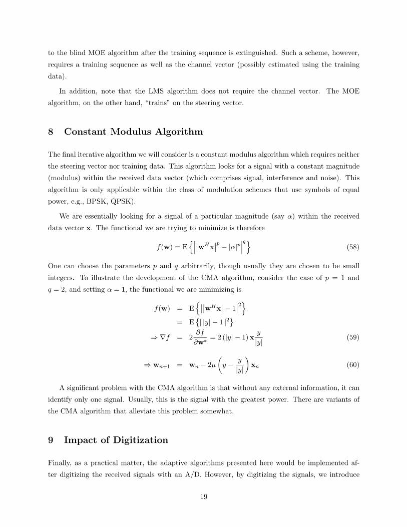
8 Constant Modulus Algorithm
The final iterative algorithm we will consider is a constant modulus algorithm which requires neither
the steering vector nor training data. This algorithm looks for a signal with a constant magnitude
(modulus) within the received data vector (which comprises signal, interference and noise). This
algorithm is only applicable within the class of modulation schemes that use symbols of equal
power, e.g., BPSK, QPSK).
We are essentially looking for a signal of a particular magnitude (say α) within the received
data vector x. The functional we are trying to minimize is therefore
f(w) = E{
∣
∣
∣
∣
∣wHx∣
∣
p− |α|p
∣
∣
∣
q}
(58)
One can choose the parameters p and q arbitrarily, though usually they are chosen to be small
integers. To illustrate the development of the CMA algorithm, consider the case of p = 1 and
q = 2, and setting α = 1, the functional we are minimizing is
f(w) = E{
∣
∣
∣
∣wHx∣
∣ − 1∣
∣
2}
= E{
| |y| − 1 |2}
⇒ ∇f = 2∂f
∂w∗= 2 (|y| − 1)x
y
|y|(59)
⇒ wn+1 = wn − 2µ
(
y −y
|y|
)
xn (60)
A significant problem with the CMA algorithm is that without any external information, it can
identify only one signal. Usually, this is the signal with the greatest power. There are variants of
the CMA algorithm that alleviate this problem somewhat.
9 Impact of Digitization
Finally, as a practical matter, the adaptive algorithms presented here would be implemented af-
ter digitizing the received signals with an A/D. However, by digitizing the signals, we introduce
19

20 40 60 80 100 120 140 160 180 200
−40
−30
−20
−10
0
10
20
30
Training Symbol Number
Err
or (
dB)
LMSRLS
Figure 9: Residual error in the LMS and RLS techniques
quantization noise which has not been accounted for in our analysis. Consider a system where the
signal (x) at each element is sampled and digitized using bx bits and the weight is represented using
bz bits. Due to digitization, the signal that will be processed (x) is the true signal (x) plus some
quantization noise (nx). Similarly for the weights. Therefore,
x = x+ nx, (61)
w = w + nw. (62)
In the beamforming approach we are multiplying these two quantized values. The output y = w∗x.
y = w∗x (63)
= (w + nw)∗(x+ nx)
= w∗x+ n∗wx+ w∗nx + n∗wnx (64)
Representing as σ2x the average power in the signal x and σ2
w = E(|w|2), the useful power in the
output signal y is σ2xσ
2w. Similarly, if σ2
nx and σnw are the powers in the quantization noise terms
nx and nw, assuming independence between x and w, the average quantization noise power is
σ2xσ
2nw + σ2
wσ2nx + σ2
nwσ2nw. The signal-to-quantization-noise ration (SQNR) is therefore
1
SQNR=
σ2xσ
2nw + σ2
wσ2nx + σ2
nwσ2nw
σ2xσ
2w
(65)
=σ2nw
σ2x
+σ2nx
σ2w
+σ2nwσ
2nx
σ2wσ
2x
(66)
Now, if the dynamic range of x (w) is Rx (Rw), and one were using bx (bz) bits to discretize
the real and imaginary parts x (w), the real and imaginary parts of the quantization error nx is
20
uniformly distributed between (−∆/2,∆/2) where ∆ = Rx
2bx. The error power each the real and
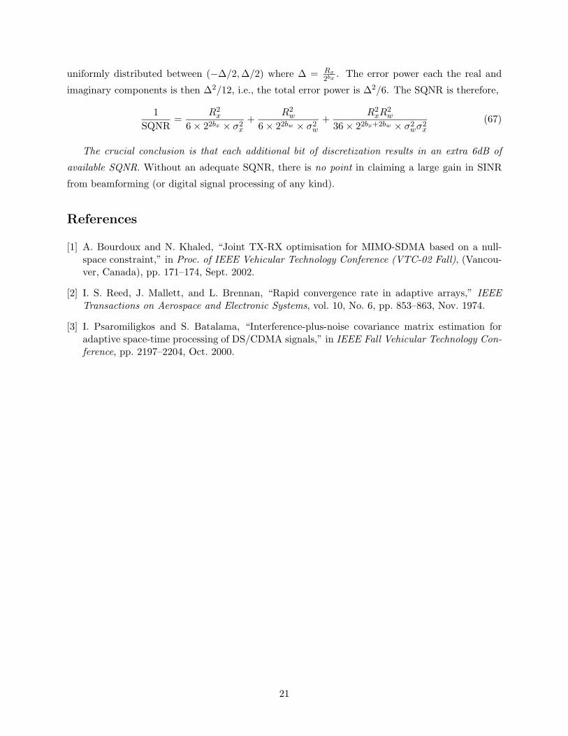
imaginary components is then ∆2/12, i.e., the total error power is ∆2/6. The SQNR is therefore,
1
SQNR=
R2x
6 × 22bx × σ2x
+R2w
6 × 22bw × σ2w
+R2xR
2w
36 × 22bx+2bw × σ2wσ
2x
(67)
The crucial conclusion is that each additional bit of discretization results in an extra 6dB of
available SQNR. Without an adequate SQNR, there is no point in claiming a large gain in SINR
from beamforming (or digital signal processing of any kind).
References
[1] A. Bourdoux and N. Khaled, “Joint TX-RX optimisation for MIMO-SDMA based on a null-space constraint,” in Proc. of IEEE Vehicular Technology Conference (VTC-02 Fall), (Vancou-ver, Canada), pp. 171–174, Sept. 2002.
[2] I. S. Reed, J. Mallett, and L. Brennan, “Rapid convergence rate in adaptive arrays,” IEEETransactions on Aerospace and Electronic Systems, vol. 10, No. 6, pp. 853–863, Nov. 1974.
[3] I. Psaromiligkos and S. Batalama, “Interference-plus-noise covariance matrix estimation foradaptive space-time processing of DS/CDMA signals,” in IEEE Fall Vehicular Technology Con-ference, pp. 2197–2204, Oct. 2000.
21


![Joint Optimal Power Control and Beamforming in …sig.umd.edu/publications/Rashid-Farrokhi_TComm_199810.pdf · A centralized power control algorithm [4], [5] solves (4) by requiring](https://static.fdocuments.in/doc/165x107/5b5e35e87f8b9aa3048c8b45/joint-optimal-power-control-and-beamforming-in-sigumdedupublicationsrashid-farrokhitcomm.jpg)