Optimal ordering and pricing strategies in the presence of a B2B spot market

Optimal Bank RegulationIn the Presence of Credit and Run Risk∗
Anil K Kashyap† Dimitrios P. Tsomocos‡ Alexandros P. Vardoulakis§
September 2017
Abstract
We modify the Diamond and Dybvig (1983) model of banking to jointly study various regu-lations in the presence of credit and run risk. Banks choose between liquid and illiquid assetson the asset side, and between deposits and equity on the liability side. The endogenouslydetermined asset portfolio and capital structure interact to support credit extension, as well asto provide liquidity and risk-sharing services to the real economy. Our modifications createwedges in the asset and liability mix between the private equilibrium and a social planner’sequilibrium. Correcting these distortions requires the joint implementation of a capital and aliquidity regulation.
Keywords: Bank Runs, Credit Risk, Limited Liability, Regulation, Capital, LiquidityJEL Classification: E44, G01, G21, G28
∗Revised version of “How does macroprudential regulation change bank credit supply?", NBER Working Paper No.20165. We are grateful to Saki Bigio (discussant), Dong Beom Choi (discussant), Emmanuel Fahri (discussant), JohnGeanakoplos, Todd Keister, Frank Smets (discussant), Adi Sunderam (discussant) and seminar participants at numerousinstitutions and conferences for comments. Kashyap thanks the Initiative on Global Markets at the University of ChicagoBooth School of Business, the Houblon Norman George Fellowship Fund, and the National Science Foundation for agrant administered by the National Bureau of Economic Research for research support. Kashyap’s disclosures of hisoutside compensated activities are available on his web page. All errors herein are ours. The views expressed in thispaper are those of the authors and do not necessarily represent those of Federal Reserve Board of Governors, anyone inthe Federal Reserve System, the Bank of England, or any of the institutions with which we are affiliated.
†University of Chicago Booth School of Business, United States and Bank of England; email:[email protected]
‡Saïd Business School and St. Edmund Hall, University of Oxford, United Kingdom;email: [email protected]
§Board of Governors of the Federal Reserve System, United States; email: [email protected]
1 Introduction
Financial intermediaries, hereafter banks, perfom various socially useful functions. These include
providing liquidity (Diamond and Dybvig, 1983), facilitating credit extension to fund productive
investment (Diamond, 1984), and improving risk-sharing (Benston and Smith, 1976; Allen and
Gale, 1997, 2004). Banks’ asset portfolio composition and liabilities structure interact to allow
them to perform these services. However, these same interactions can also be a source of fragility.
Transforming illiquid long-term assets into liquid short-term claims, such as demandable deposits,
is desirable, but exposes banks to the possibility of a run which can be disastrous for the bank, its
borrowers and its depositors. Likewise, funding risky loans through both debt and equity improves
risk-sharing (and potentially raises growth), but can lead to socially wasteful bankruptcy costs.
Finally, the presence of short-term liabilities can generate better incentives for banks to monitor
borrowers and honor their liabilities (Calomiris and Kahn, 1991; Diamond and Rajan, 2001), but
creates run risk that long-term funding avoids.
In this paper we expand the Diamond and Dybvig (1983) model of banking to incorporate all
of the three aforementioned banking functions and explore whether private decisions result in an
efficient level of intermediation. Our analysis is related to the emerging literature exploring optimal
macroprudential regulation to address various inefficiencies, such as aggregate demand externalities
in the presence of nominal rigidities (Farhi and Werning, 2016), pecuniary externalities operating
through collateral constraints (Bianchi and Mendoza, forthcoming) or fire-sales externalities (Stein,
2012). However, our focus is different as we are interested in identifying externalities that pertain
to banks choices associated with endogenous credit risk and run risk.
Bankers have a comparative advantage at intermediating funds, but their incentives to monitor
their investment can differ from their investors due to private benefits that are available to them. On
one hand, a fragile funding structure and run risk can be optimal to discipline the banker and align
the incentives for monitoring. Thus, short-term debt is preferred to long-term funding for its disci-
plining function even when both are able to provide liquidity services through retrading in capital
markets. On the other hand, a fragile funding structure can misalign the incentives between bankers
and debt-holders in the presence of credit risk and, hence, result in both distorted asset holdings
and a capital structure. Contrary to the case of pure run risk, equity financing has an advantage
over short-term debt in dealing with externalities from the management of credit risk. Overall,
run and credit risk endogenously interact to determine banks’ asset portfolio and capital structure,
which, in turn, has implications for the level of intermediation and the allocation of benefits from
intermediation.
We make five modifications to the original Diamond-Dybvig model to capture the aforemen-
tioned interaction of credit and run risk. First, bank loans are risky. The risk arises because borrow-
ers use the bank funding to invest in a technology where the payoff is uncertain and the results are
private information for the borrower.
Because loans are risky, borrowers can default due to insufficient funds. This can potentially
cause the bank to be unable to fully repay depositors who incur additional bankruptcy costs. Our
2
second modification is to assume that both banks and borrowers are subject to limited liability.
Third, the private information about a borrower’s success leads banks to have to monitor the
borrower. The banks are run by bankers who seek to maximize the value of dividends they receive
from the banks. Absent monitoring, the bankers enjoy a private benefit, but without monitoring,
their borrowers will never repay their loans.
Fourth, a full set instruments to insure against all risks in the environment is unavailable. Both
loan and deposit contracts cannot be made contingent on the aggregate realization of risks. As a
result, credit risk occurs in equilibirium. Moreover, contracts can be incomplete such that not all
actions of borrowers are ex-ante contractible. For example, a more comprehensive debt contract
would not only specify an interest rate and a debt amount, but also the composition and amount of
assets that can be seized if default occurs. Likewise, bankers choose how much equity to contribute
to the bank in addition to accepting deposits. Not only the asset portfolio, but also the capital
structure of the bank is endogenously determined.
Fifth, we assume that depositors receive signals about the value of loans that the bank can
recover before they are due. This interim liquidation value is available to pay depositors who are
seeking to withdraw. We suppose that the depositors make a decision whether to run based on these
signals. Our assumption about the nature of these signals means that the decision to run depends
on the asset and liability structure of the bank, and the value of the signal. There is a unique signal
threshold that determines whether there is a run.
There are three important consequences of these modifications. First, they create an environ-
ment where the level of credit risk and run risk in the economy are endogenously determined and
interact. Second, the bank’s choices of both the mix between the level of liquid and illiquid assets
and between debt and equity differ from what a social planner would select. The private equilibrium
features excessive levels of lending relative to liquid asset holding and more debt financing relative
to equity financing. Because of the market incompleteness, there is not a unique social planner’s
allocation. Instead the preferred allocations will depend on the planner’s weights on the different
actors in the economy. Loosely speaking, when the planner favors the savers, she will choose to
limit risk while emphasizing liquidity provision for depositors. Alternatively, if the planner is pri-
marily looking out for borrowers, the allocations are arranged to control run risk while increasing
lending.
The third outcome of the model is to study whether regulations akin to those embedded in
the new Basel regulations for liquidity and capital could align the private asset and liability mix
with the social efficient one. In particular, we study two capital regulations–one that ties capital
requirements to the riskiness of bank assets and a second leverage requirement that is determined
by the total scale of bank assets. We also look at a pair of liquidity regulations. One, akin to the
so-called liquidity coverage ratio, makes the bank hold more short-term liquid assets when it uses
more runnable funding. The other, like the so-called net stable funding ratio, requires the bank to
increase its long term funding to match its longer term assets.
Although regulations can individually reduce the probability that a run occurs and improve
3
welfare, they affect the asset mix and the liability mix in different ways. Capital regulations result
in more lending, but in lower liquid asset holdings than socially optimal. In contrast, liquidity
regulations reduce lending, but leave the level of capital below the social optimum. Because the
private allocations diverge from the socially optimal allocations in two ways, no single regulation
is sufficient to implement the social optimum; we show that at least two tools are needed. Yet,
the optimal regulatory mix cannot arbitrarily include any two tools, because some regulations may
be redundant. For example, we find that the two liquidity regulations cannot be jointly binding.
Nevertheless, combinations of a capital and a liquidity regulation are feasible and are sufficient to
implement the social planner’s solution.
A special case arises when bankers have ample wealth to invest in so much bank equity, which
pushes their economic surplus down to zero in equilibrium. Therein, planning outcomes are de-
centralized with only one regulation, which depends on the deadweight losses in bankruptcy. If
the latter are low, then only liquidity regulation is needed, while for high ones, capital regulation is
used.
The remainder of the paper is separated into four parts. In section 2, we describe the model
and show the privately optimal choices for the bank, the savers and the entrepreneurs. In section 3
we study the efficient allocations chosen by a social planner and derive expressions for the wedges
between the private and social decisions. In section 4, we explore how regulation can be used to
correct the private inefficiencies. The following section analyzes a special case where less regulation
is needed. Section 6 concludes by summarizing the main findings, reiterating the intuition for them,
and describing a few directions for future research. Additional derivations and model extensions are
relegated to an online appendix.
2 Model
The model consists of three periods, t = {1,2,3}, features a single consumption good and includes
three types of (representative) agents; an entrepreneur (E), a saver (S) and a banker (B). The en-
trepreneur has access to a productive, but illiquid, risky technology. The entrepreneur’s primary
decision is how much of her own money to allocate to the project and how much to borrow.
Funds invested at date 1 yield an uncertain payoff A3s ·F (·) at date 3 depending on the realization
of state s, where F is a concave production function and A3s a productivity shock. State s = {g,b}occurs with probability ω3s and these states represent a good and a bad realization of the shock, i.e.,
A3g > A3b. The project delivers no output at date 2 but it can be liquidated. The liquidation value,
ξ, is uncertain and independent of the productivity shock.1
The banker manages an institution which we call a bank that acts as an intermediary between the
1The discrete state space for the productivity shock is not important for our results, but it facilitates the computationof the numerical equilibria. As described below, all agents have linear preference at t = 3, so that they care only aboutthe expected payoffs and not the state by state payoffs. Moreover, another shock will be realized at t = 2, which followsa continuous distribution and is independent of the realization of the productivity shock. Thus, from the perspective oft = 1, there is an “infinite" dimensional state space in the future. We are more precise below.
4

entrepreneurs and savers. The bank is funded partly from the banker’s endowment and by raising
addtional funds from the saver. The funds raised at date 1 are invested into either a liquid storage
asset or a loan to the entrepreneur, which the bank can recall in the intermediate period. Moreover,
the banker decides whether to monitor the entrepreneur’s project at t = 3 or not. Monitoring is
important because the productivity shock is private information to the entrepreneur.
The saver has a large endowment at date 1 that is used to fund initial consumption and savings.
The savers have uncertain future consumption needs and, as in Diamond and Dybvig (1983), after
date 1, some fraction will need to consume at t=2 and the rest can wait to consume at date 3. The
saver invests in bank deposits or holds a liquid storage asset. The deposits are demandable, which
is important to provide incentives to the banker to monitor as we describe in detail later.2
The liquidation value, ξ, follows a uniform distribution U ∼[ξ,ξ]
with 0 ≤ ξ < 1 < ξ and
∆ξ = ξ− ξ. The fact that ξ can exceed 1 will be important in what follows. We assume that long-
term loans are callable in which case the entrepreneur forfeits the portion of the project that is
funded by the loan. Moreover, when a project is liquidated it yields an immediate gross return ξ.
The liquidation value can be justified in several ways. For instance, the incomplete project could
have a secondary use in the interim period because it can be used in conjunction with alternative
short-term technology. Or, we could assume that it can be sold to some outside investors as in
Shleifer and Vishny (1992). In other words, ξ does not strictly represent the salvage value of the
long-term investment, as for example in Cooper and Ross (1998), but rather the liquidation/resale
value of long-term investment. ξ has to be high enough that the bank can always withstand a panic
for some realizations. Yet, ξ has to be low enough that the bank may run out of liquidity even if a
panic does not occur. We describe the importance of these bounds in section 2.4.3
Sections 2.1-2.4 describe in detail the agents’ optimization problems in the private equilibrium.
As we introduce the agents’ problems, we emphasize the reasons why individual agents will make
choices that would differ from a social planner. Section 2.5 discusses the key modeling assumptions.
2We assume that savers cannot buy equity in the bank in order to simplify the exposition of our baseline model. Inthe online appendix, we present a more complicated model where where the bank raise both inside equity from bankersand outside equity from savers. Therein, the bank shares purchased by savers are tradable in a frictionless market in theintermediate period and, thus, also provide liquidity services. Although bank equity can also provide liquidity services,because it can be traded in a secondary market similar to Jacklin (1987), an all-equity funding structure would not beoptimal in even in this richer setup due to the disciplinary role of runnable debt. Overall, the main results from the modelin the body of the paper continue to hold.
3Our model can easily be adjusted to make the liquidation value depend on the expected value of the loans, i.e,ξ ·EsV I
3s(1+ rI), where V I3s is the percentage repayment on the loan given by (15) later and rI is the loan rate. Then,
ξ would capture the fraction (between 0 and 1) of the expected value that can be obtained at liquidation. The expectedvalue is computed over the possible realizations of state s in the last period for known probabilities ω3s. The liquidationvalue, ξ ·EsV I
3s(1+ rI), would vary because ξ varies. Given that the expected value of loans is higher than one, the twoapproaches would yield qualitatively similar results. Alternatively, we could have assumed that ξ does not vary, but theprobability distribution ω3s varies as in Goldstein and Pauzner (2005). Then, the liquidation value would continuouslyvary with the realization of the true probability distribution ω3s because EsV I
3s(1+ rI) varies. The upper and lowerdominance regions in the incomplete information game would still be endogenously determined in these cases.
5
2.1 Savers
The savers are endowed with eS1 and eS
2 at t = 1 and t = 2, respectively. In the initial period, they
invest in bank deposits, D, and can additionally save by investing in the liquid storage technology,
LIQS1. A portion of savers, δ, receive a preference shock to consume in the intermediate period,
while the rest, 1− δ, want to consume at t = 3. The preference shock is private information, i.i.d.
and is not contractible ex-ante.
Deposits are demandable, early withdrawals are serviced sequentially and the interest rates, rD2
and rD3 , for withdrawals at t = 2 or t = 3 respectively, are uncontingent. This contract structure
creates the possibility of a run, since patient savers may choose to demand their deposits early
depending on their own information and their expectations about the actions of other patient savers;
every (patient) depositor receives a noisy signal at t = 2 about the liquidation value, ξ, of the bank’s
loans and there is a threshold, ξ∗, determining whether a patient saver decides to run or keep her
deposits in the bank. The probability of a run will be unique and depend on fundamentals similarly
to Goldstein and Pauzner (2005).4
In order to facilitate the exposition of the model, while retaining precision, we denote all vari-
ables that are not (pre-)determined at t = 1 as functions of the liquidation value, ξ, and the portion
of savers who decide to withdraw at t = 2, λ∈ [δ,1]. In equilibrium, either all savers choose to with-
draw, λ = 1, or only the impatient savers withdraw, λ = δ. However, the out-of-equilibrium beliefs,
which play an important role in the determination of the run probability derived below in section
2.4, depend on the conjectured portion of savers withdrawing. This conjecture can be anywhere
between δ and 1.
It is instructive to review the different possible scenarios separately. If there is no run, only
impatient depositors withdraw and they receive the full amount of promised payment, D(1+ rD
2).
Patient depositors’ repayments are determined as a function of the technology shock in the next
period. In a run, all depositors attempt to withdraw and there is probability θ(ξ,1) that a depositor
is served.5 Conditional on the bank surviving to t = 3 patient depositors receive their promised
payment in full or in part if the bank defaults, V D3s(ξ,δ)D
(1+ rD
3). The percentage repayment on
4Bank-runs in our model can also be panic based rather than purely information based as in Chari and Jagannathan(1988), Jacklin and Bhattacharya (1988), Allen and Gale (1998), Uhlig (2010), Angeloni and Faia (2013), Boissay,Collard and Smets (2016). In other words, a bank-run can occur due to a coordination problem among depositors evenif the bank is solvent in the long-run. Similarly, a bank-run can also occur because the information about fundamentalsis very bad. In determining the optimal ex-ante decisions, it is important to know what determines panics. In theDiamond-Dybvig model panics are a multiple equilibrium outcome. Cooper and Ross (1998), Peck and Shell (2003)and Keister (2015) suppose instead that the probability of a bank-run is driven by sunspots. In our earlier working paperKashyap, Tsomocos and Vardoulakis (2014), in Gertler and Kiyotaki (2015) and in Choi, Eisenbach and Yorulmazer(2016) the probability of a run is determined by an exogenous function of key fundamentals. Ennis and Keister (2005)take an axiomatic approach to equilibrium selection and link the probability of a particular equilibrium being playedto appropriately defined incentives of agents. Instead, we use the global games approach developed by Morris andShin (1998) and applied to banks runs by Goldstein and Pauzner (2005) to derive a unique probability of run whichdepends on fundamentals. Although we maintain they key assumption in Goldstein and Pauzner (2005) to obtain a uniqueequilibrium, we amend their approach by introducing noisy signals on a different variable so that the upper dominanceregion is endogenously derived rather than assumed. Rochet and Vives (2004) and Vives (2014) also take a global gameapproach, but delegate the withdrawal decision to a (deposit) fund manager with a simpler payoff function.
5This probability is determined by equation (12), derived in section 2.2. In a run all savers attempt to withdraw, λ = 1.
6

period 3 deposit withdrawals, V D3s(ξ,δ), is given by equation (16) that is derived below. Depositors
have to pay an additional cost, cD, per unit of promised payments to receive a payment when the
bank defaults.
Thus, the net repayment on deposit is(V D
3s(ξ,δ)− cD · Id)
D(1+ rD
3), where Id is an indicator
function that takes the value of 1 when the bank defaults.
We proceed by formally presenting savers’ problem. Savers’ consumption at t = 1 is given by
c1 = eS1−D−LIQS
1. (1)
Given the various cases that occur in the latter periods when the savers may or may not be
patient, choose to withdraw or run, and be paid or not in a run, it is helpful to introduce some further
notation. Denote by j = i, p the saver’s type, which is realized at t = 2. They will be impatient
( j = i) with probability δ and patient ( j = p) with probability 1−δ. A run occurs when ξ ∈[ξ,ξ∗
].
In this case, all savers attempt to withdraw, but only a fraction of them are repaid. We denote by
Iθ an indicator which takes the value of 1 if an individual saver is repaid, where the (endogenous)
probability of repayment is θ(ξ,1). Then, the consumption of a saver of type j is given by
cts ( j,Iθ) = Iθ ·D(1+ rD
2)+LIQS
1 + eS2, (2)
where ts = 2 for j = i and ts = 3s for j = p, because patient savers still only consume at t = 3 and
will transfer their resources from period 2 to 3 using the storage technology.
We also define an indicator Iw which takes the value of 1 if an agent of type j withdraws when
a run does not occur, i.e., when ξ ∈[ξ∗,ξ], and is 0 otherwise. Her consumption is denoted by
cts ( j,Iw). Although in equilibrium patient savers will truthfully report their type and only impatient
savers will withdraw, we need to contemplate deviations where a patient saver could opt to withdraw
and show that such deviations never are optimal (see section 2.4). The consumption of an impatient
saver is then given by
c2 (i,Iw = 1) = D(1+ rD
2)+LIQS
1 + eS2. (3)
The consumption at t = 3 of a patient saver who chooses to wait or withdraw are, respectively, given
by
c3s (p,Iw = 0) =(V D
3s (ξ,λ)− cD · Id)
D(1+ rD
3)+LIQS
1 + eS2, (4)
or c3s (p,Iw = 1) = D(1+ rD
2)+LIQS
1 + eS2. (5)
Note that in equilibrium, λ = δ in (4).
Finally, short-selling of deposits and the liquid asset is not allowed. So, in solving the model we
add the following constraints (with the associated Lagrange multipliers indicated in parentheses):
D≥ 0 (νD); and LIQS1 ≥ 0 (νLIQS
1).
The savers choose the level of deposits and their holdings of the liquid asset to maximize their
7
utility subject to constraints (1)-(5). The expected utility of a representative saver is given by
US =U1 (c1)+ ∑t=2,3
run︷ ︸︸ ︷∫
ξ∗
ξ
E j,θUt (cts ( j,Iθ) ; j)dξ
∆ξ
+
no run︷ ︸︸ ︷∫ξ
ξ∗E j,sUt (cts ( j,Iw) ; j)
dξ
∆ξ
. (6)
Conditional on a run occurring, patient savers compute the expected utility from remaining
patient or attempting to withdraw and probabilistically receiving payment on their deposits (E j,θ).
If a run does not occur, patient savers compute the expected utility from withdrawing early, and
from receiving the state contingent payment on deposits (E j,s). Note that we have indexed the
utility function by the time t and agent type j. Impatient savers receive utility only at t = 2 which
is discounted to the present by β < 1, while patient savers receive utility only at t = 3 which is
discounted to the present by β2. Moreover, we assume that savers have quasi-linear preferences; at
t=1 and at t = 2 (for j = i) savers have concave utility U , while savers have linear preferences at
t = 3 (for j = p).6
An individual saver takes the probability of being repaid in a run, θ(ξ,1) and the percentage re-
payment, V D3s(ξ,δ), as given. These objects depend on the aggregate bank portfolio and we suppose
that the individual saver is sufficiently small so as to not account for her impact on them. A social
planner would internalize the effect of the choices.
The optimal supply of deposits by savers is given by:
DS :−U ′1 (c1)+(1+ rD
2)
run︷ ︸︸ ︷∑
t=2,3
{∫ξ∗
ξ
θ(ξ,1) ·E jU ′t (cts ( j,1) ; j)dξ
∆ξ
}+
no run, impatient︷ ︸︸ ︷δ
∫ξ
ξ∗
U ′2 (c2 (i,1) ; i)dξ
∆ξ
+(1−δ)
∫ξ
ξ∗ ∑
sω3sU ′3 (c3s (p,0) ; p) ·
(V D
3s (ξ,δ)− cD · Id)· (1+ rD
3 )dξ
∆ξ︸ ︷︷ ︸no run, patient
+νD = 0. (7)
Condition (7) says that savers equate the marginal utility of forgone consumption at t = 1 to the
expected marginal utility gain from holding deposits in the future. In a run, all savers withdraw;
their marginal utility depends on their type, j, and the probability that they are repaid, θ(ξ,1). If a
run does not occur, impatient savers are fully repaid at the promised rate, 1+rD2 , while patient savers
do not withdraw and receive the uncertain deposit payoff, V D3s(ξ,δ) ·
(1+ rD
3), minus any marginal
bankruptcy costs.
Savers may want to self-insure and hold the liquid asset. The optimal liquid holdings, LIQS1, are
6The linearity of utilities in the final period is not important for our results and we have assumed it for simplicity ofexposition. We discuss further this assumption in section 2.5.
8

given by:
−U ′1(c1)+ ∑t=2,3
run︷ ︸︸ ︷∫
ξ∗
ξ
E j,θU ′t (cts ( j,Iθ) ; j)dξ
∆ξ
+
no run︷ ︸︸ ︷∫ξ
ξ∗E j,sU ′t (cts ( j,Iw) ; j)
dξ
∆ξ
+νLIQS1= 0. (8)
Condition (8) says that holding the liquid asset allows the saver to self-insure against states that she
is not repaid in a run, i.e., compared to using a deposit as in (7) the liquid asset always delivers
future consumption, but does so by forgoing the higher uncertain return that deposits promise.
Moreover, note that the equilibrium outcomes will be incentive compatible, i.e., a patient saver
will not have an incentive to misrepresent her type and withdraw for ξ > ξ∗. This is guaranteed by
the way the run threshold is determined, which we describe in detail in section 2.4.
Finally, we need to specify what would happen if the savers chose to avoid using the bank. One
possibility is that they save using only the liquid asset. We refer to this as autarky. The liquidity
choice in this case is the solution to U ′1(eS1−LIQS,aut
1 )+∑t=2,3 E jU ′t (eS2 +LIQS,aut
1 ; j) = 0. These
holdings imply a utility in autarky US,aut , which is a useful benchmark for gauging the benefits that
intermediation delivers through liquidity provision. A second alternative is that the savers could
attempt to directly lend to entrepreneurs (assuming that they would also have to monitor after doing
so). We denote the resulting level of utility by by US,dl . The participation constraint of savers is,
then, given by:
US ≥max(
US,aut ,US,dl). (9)
Given that this constraint will mostly not bind for the results we present, we report the detailed
problem when savers lend directly to entrepreneurs in the online appendix. We will be explicit about
the occasions that the constraint binds.
2.2 Bankers and Banks
The banker makes all investment and funding decisions to maximize her own utility. At t = 1, she
is endowed with eB and decides how much equity, E, to put into the bank. Her utility is given by:
UB = γ ·U(eB−E
)+
no run︷ ︸︸ ︷∫ξ
ξ∗ ∑
sω3sDIV3s(ξ,δ)
dξ
∆ξ
, (10)
where DIV3s are the dividends in state s at t = 3.
The banker trades off foregoing current consumption to investing in equity and receiving div-
idends in the future. The banker has also quasi-linear preferences and the same utility function at
t = 1 as the savers, but unlike the saver, never needs to consume in the interim period. We have
maintained the linearity of preferences at t = 3, though we restrict parameters so that savers never
9

insure the banker against future uncertainty.7
Additionally, the banker chooses how many deposits to raise, D, and using the total funds, the
banker invests in the liquid assets, LIQ1, and illiquid loans, I. The loan contract is uncontingent and
requires a payment of 1+ rI per dollar of lending at t = 3. As already mentioned, loans are callable
at any time before maturity at which case the entrepreneur surrenders the projects funded by these
loans and does not have an obligation to repay them at t = 3.
The balance sheet constraint at t = 1 is given by:
BS : I +LIQ1 = D+E. (11)
We define ψBS to be the multiplier on the balance sheet constraint (11), which represents the shadow
value of funding, i.e., the endogenous cost of expanding assets by raising a unit of funds.
The balance sheet and profits after t=2 depend on the realization of ξ and the number of people
withdrawing, λ. If a bank-run occurs then the bank is liquidated and the proceeds are distributed
according to sequential service constraint. Thus, the probability that any saver is served is equal to
θ(ξ,λ) =LIQ1 +ξ · I
λ ·D · (1+ rD2 )
. (12)
If the bank survives the run, it will have to recall and liquidate a portion y(ξ,λ) of its loan
portfolio to serve the early withdrawals given by
y(ξ,λ) =λ ·D · (1+ rD
2 )−LIQ1 +LIQ2 (ξ,λ)
ξ · I, (13)
where LIQ2 (ξ,λ) ≥ 0 are the liquid holdings carried over to the third period. Our assumptions
regarding the distribution of ξ lead bank to hold insufficient liquid assets to service all early deposit
withdrawals even when only the impatient savers withdraw. So the bank is always planning to call
some loans. In principle, the bank could want to liquidate its whole loan portfolio and carry the
proceeds forward using the storage technology, but this would only be the case if the realization
of ξ is higher than the expected return from holding the loan to maturity, which we have excluded
by assumption. As a result, y(ξ,λ) will take interior values between zero and one, and it will be
decreasing in ξ and increasing in λ for a pre-determined bank portfolio.
Conditional on the bank surviving, the dividends depend on the portion of the portfolio liqui-
7The difference between the banker and the savers expected utility is that the former values future consumptionmore than current or in other words γ < 1. Assigning to the banker the same utility function requires high enough eB
or low enough γ such that she would be willing to invest enough of her own wealth in equity to provide risk-sharingbenefits to savers. We do the second because we want the banker endowment to represent only a small part of thetotal endowment in the economy, with the vast majority accruing to the savers. For γ = 1/β
2, such that savers and thebanker discount the future the same way, and for logarithmic utility, we can obtain the same equilibrium for banker’swealth eB = E +(eB−E)/(β2
γ), where E is the equilibrium value of contributed equity. Finally, given that bankers areprotected by limited liability and that future endowments are not contractible, quasi-linear preferences allow us to excludefinal period endowments from our analysis by setting them to zero.
10
dated y(ξ,m) and are given by
DIV3s (ξ,λ) = (1− y(ξ,λ)) ·V I3s (ξ,λ) · I ·
(1+ rI)+LIQ2 (ξ,λ)−V D
3s (ξ,λ) · (1−λ) ·D ·(1+ rD
3),
(14)
where V I3s (ξ,λ) is the percentage repayment on the remaining risky loans. It is given by
V I3s (ξ,λ) = min
[1,
A3sF(IE +(1− y(ξ,λ) · I)
)(1− y(ξ,λ)) · I · (1+ rI)
](15)
and V D3s (ξ,λ) is the repayment rate on deposits. It is given by
V D3s (ξ,λ) =
[1,(1− y(ξ,λ)) ·V I
3s (ξ,λ) · I ·(1+ rI
)+LIQ2 (ξ,λ)
(1−λ) ·D ·(1+ rD
3
) ]. (16)
In other words, bank profits in (14) are equal to the revenue received from the repayment on the
outstanding loans plus any liquid assets carried forward minus the repayment on the deposits that
were not withdrawn early. Equation (15) says that the loan is fully repaid when the revenue available
to the entrepreneur, which is derived from the own funds invested by the entrepreneurs, IE , and
bank loans, is higher than the outstanding loan obligation; otherwise the entrepreneur defaults and
the bank seizes everything that is available. Equation (16) says that late depositors are repaid in full
when the value of bank assets is higher than the promised deposit payments; otherwise the bank
defaults and depositors divide the assets in a pro-rata fashion.
After the run uncertainty has been resolved and the true value of ξ is learned, the banker can
choose to monitor the borrower to learn the true value of the productivity shock at t = 3, which
is private information to the entrepreneur. Alternatively, the banker can forgo the monitoring and
enjoy a private benefit from running the bank. We follow the long tradition in the literature assuming
that monitoring is costly for the banker because she would have to give up a private benefit she would
otherwise receive from managing the bank (see, for example, Holmström and Tirole, 1997). This
assumption creates an ex-post moral hazard problem in which the banker will choose to monitor
only if the expected dividends are higher than the private benefit. If the banker opts not to monitor,
the entrepreneur would always report the lowest realization of the productivity shock and default on
the loan.8 The banker will choose to monitor for all ξ≥ ξ∗ if the following incentive compatibility
constraint is satisfied:
IC : ∑s
ω3sDIV3s(ξ∗,δ)−PB≥ 0, (17)
where PB is the private benefit.
The first term in the IC constraint is the expected payoff to the banker if she monitors when
ξ = ξ∗. We take the expectation because the banker has to decide whether to monitor before she
8The productivity level is common across projects. Therefore, as in Diamond (1984), monitoring costs are conservedby having a bank monitor all borrowers, relative to having individual lenders monitor individual borrowers. Thus, thebank monitoring expands the supply of credit.
11

learns the true value of A3s. The second term is the private benefit. If the banker does not monitor,
then the entrepreneur reports the lowest realization for A3s, defaults on the loan repayment and
forces the bank to default on its deposits (so that bank equity is worthless). It suffices that the IC
constraint is satisfied for ξ = ξ∗, because expected dividends are increasing in ξ, thus the banker
will always have an incentive to monitor if there is no run.
The bank and the depositors may want to write a deposit contract not only on the deposits rate(s)
and the amount of deposits, but also over all the factors affecting the riskiness of the deposits. These
risks are governed by all aspects of the bank’s balance sheet, in particular, its choice of leverage (or
equivalently a capital ratio), its asset allocation between loans and liquid assets (i.e., a liquidity ratio)
and its maturity mismatch (i.e., a net stable funding ratio). However, such comprehensive contracts
may not be possible for a number of reasons and do not resemble observed deposit or unsecured
funding arrangements in reality.9 As a result, the bank would be tempted to deviate in the way it
chooses its leverage, liquidity and maturity mismatch after it has entered into a deposit contract and
received the deposits. Technically, this lack of commitment means that the bank will optimize only
over states of the world in which it is solvent because it is protected by limited liability. Likewise,
it will only internalize how it affects the supply of deposits when it chooses the contract terms(D,rD
2 ,rD3). The bank does understand that taking more risk increases the cost of raising deposits,
and would ideally want to promise depositors that it will behave prudently. But, after the deposit
contract has been signed, the bank has an incentive to deviate towards lending more, holding fewer
liquid assets and raising less equity.
Depositors have rational expectations and ex-ante require that the bank offers higher deposit
rates to compensate for the anticipated risk-taking due to the lack of commitment. In contrast, a
social planner would recognize that the bank’s insolvency adversely impacts savers, and would ac-
count for this in making allocations. We believe that incomplete contracting is an important feature
of reality when financial institutions have a rich balance sheet and their activities expose savers
to credit risk. Nevertheless, we also examine the case where comprehensive contracts, specifying
the full set of choices made by the banker, can be written. We denote by Ic an indicator function,
which takes value one if deposit contracts are comprehensive and zero if they are incomplete. Our
conclusions regarding the need for bank regulation hold for both cases.
One force in the model that partially disciplines the banker is the possibility of a bank run. The
banker will internalize how her investment and funding choices affect the probability of a run via
condition (32) (that is derived below), and hence the probability that she will make profits. Similarly,
the banker understands that her ex-post incentives to monitor need to be consistent with condition
(17); otherwise depositors would anticipate that the banker will not have an incentive to monitor
and would always run at t = 2 driving the banker’s rents to zero. In this respect, the run risk creates
9For example, Dewatripont and Tirole (1994) argue that individual depositors are sufficiently small and diverse toenforce comprehensive contracts which discipline all banking choices. See also Stiglitz and Weiss (1981), Matutes andVives (2000), Boyd and De Nicoló (2005) among others for models with risk-taking incentives when loan contracts arenot comprehensive. Contrary to these papers, which maintain the price-taking assumption for the borrowing rate, weallow borrower to optimally choose all the terms specified in the contract.
12

an incentive for the banker to monitor its borrowers and to prudently choose its capital structure and
amount of lending at t = 1 (see Calomiris and Kahn, 1991, Diamond and Rajan, 2000, 2001).
Overall, the banker will understand how the investment and funding decision matter for future
behavior by savers and will take equations (32) and (17) as additional constraints in her optimization
problem, but she neglects the other effects of her decisions on savers and entrepreneurs utilities given
by (6) and (26).
In solving for bank’s optimal choices, we will focus on equilibria such that the bank is always
solvent in state g and always defaults in state b for all realizations of ξ ≥ ξ∗.10 Substituting into
(10) equations (13), (14), (15), (16), the banker optimizes over the risky loan, I, the liquid asset
holdings, LIQ1 and LIQ2(ξ,δ) for each ξ, the equity contributed, E, the run threshold, ξ∗, the level
of deposits, D, and the deposit rates, rD2 and rD
3 . She takes (11), (17) and (32) as constraints in her
problem. The last constraint is the global game condition, GG, which determines the run threshold
is derived in section 2.4 below. Due to limited liability the banker will only consider the states in
which she is solvent.
The optimality condition for loans, I, is:
dUB
dI−ψBS +ψIC
dICdI
+ψGGdGG
dI+ψDS
dDSdI· Ic = 0, (18)
where dUB/dI =∫ ξ
ξ∗{
ω3g(1+ rI
)}dξ/∆ξ is the marginal effect of investment on banker’s share
of profits and ψBS, ψIC, ψGG and ψDS are the multipliers on constraints (11), (17), (32) and (7)
respectively.
The expression (18) says that optimal level of lending is determined by having the banker trade
off the marginal return accruing to her against the shadow cost of funding additional lending and
the way it affects the incentive compatibility and the run threshold determination constraints. As
already mentioned, the banker only internalizes states where she is solvent due to limited liability.
Finally, the banker considers how her investment decisions affects the deposit supply only when
the level of investment is a contractual deposits term at which she can commit to. Equation (18)
corresponds to the loan supply schedule, denoted by LS, offered to entrepreneurs.
The optimality condition for first period liquid assets, LIQ1, is:
dUB
dLIQ1−ψBS +ψIC
dICdLIQ1
+ψGGdGG
dLIQ1+ψDS
dDSdLIQ1
· Ic = 0, (19)
where dUB/dLIQ1 =∫ ξ
ξ∗{
ω3g(1+ rI
)/ξ}
dξ/∆ξ is the marginal effect of liquidity on banker’s
share of profits. The optimal choice of liquid assets is governed by the same considerations to
determine optimal lending. The only difference is that the marginal return on the liquid assets is
scaled by the liquidation value ξ, because the bank needs to liquidate 1/ξ fewer loans to serve early
10Equivalently, entrepreneurs default on their loan in state b and deliver fully in state g. We have also solved themodel with more states for the realization of the productivity shock, such that entrepreneurs’ default does not need tocoincide with banks’ default. Given that our result continue to hold, we have chosen to present the model with two levelof productivity to simplify the analysis and present the more complicated case in an online appendix.
13
withdrawals for each additional unit of the liquid asset.
The banker will optimally choose the run threshold, ξ∗, which yields:
dUB
dξ∗ +ψIC
dICdξ∗ +ψGG
dGGdξ∗ +ψDS
dDSdξ∗ · Ic = 0, (20)
where dUB/dξ∗ = −∑s ω3sDIV3s(ξ
∗,δ)/∆ξ. In making this choice, (20) says that the banker bal-
ances the reduction in dividends because of a marginally higher ξ∗ against the effect from relaxing
the IC and GG constraints (and DS if the run threshold is a deposit contract term).
The optimal choice of liquidity holdings, LIQ2(ξ,δ) is made after the run uncertainty is resolved
and depends on the realization of ξ. As a result, the banker will only consider the effect on (her)
profits, but not the effect on the run threshold due to the inability to commit. Banks may want patient
investors to think that they will hold liquid assets from t = 2 to t = 3 to reduce the probability of
a run, but if the bank survives, then banks may not have an incentive to hold liquid assets because
they only care about states in which they are solvent (unless the deposit contract specifies the level
of second period liquid assets for every realization of ξ). Under incomplete contracts, the banker
will carry liquidity in period 3 only if the liquidation value is higher than the expected loan return
in the states that the bank is solvent, i.e., if ξ > ω3g(1+ rI). In the equilibria we examine this is
never the case, because ξ < 1+ rI , so it is optimal for the bank to recall loans only to serve early
withdrawals and not to hoard liquidity.
The optimality condition with respect to contributed equity, E, is:
dUB
dE+ψBS = 0, (21)
where dUB/dE = −γ ·U ′(eB−E
). Condition (21) says that injecting more equity requires the
banker to give up consumption in the initial period in exchange for increasing the funds of the bank.
Note the condition does not include a term for the effect of additional equity on constraints GG or
IC (as well as DS for comprehensive contracts). This is true because, E does not appear directly
in (32), (17) or (7), but this doesn’t mean that equity is irrelevant for their determination. On the
contrary, equity issuance can affect the run probability, the incentives to monitor and the deposit
supply through its joint determination with the other equilibrium variables.
Condition (21) governs the shadow cost of funds ψBS, which is inversely related to the amount
of equity the banker puts in the bank. In banking models without endogenous credit or run risk, the
higher funding costs of injecting more equity would feed in higher loan rates and lower investment.
This does not need to be true when equity changes the level of credit and run risk as in our model;
higher equity and cost of funding can be compatible with lower loan rates and more investment.
Finally, the banker chooses the deposit contract(D,rD
2 ,rD3)
which needs to lie on the deposit
14
supply curve (7). The optimal deposit contract satisfies the following first-order conditions:
dUB
dD+ψBS +ψIC
dICdD
+ψGGdGGdD
+ψDSdDSdD
= 0 (22)
dUB
drD2+ψIC
dICdrD
2+ψGG
dGGdrD
2+ψDS
dDSdrD
2+νrD
2= 0, (23)
dUB
drD3+ψIC
dICdrD
3+ψGG
dGGdrD
3+ψDS
dDSdrD
3= 0, (24)
where dUB/dD = −∫ ξ
ξ∗{
ω3g(1+ rI
)(δ(1+ rD
2))
/ξ+(1−δ)(1+ rD
3)}
dξ/∆ξ captures the effect
of deposits, dUB/drD2 = −
∫ ξ
ξ∗{
ω3g(1+ rI
)(δ ·D)/ξ
}dξ/∆ξ the effect of the early deposit rate
and dUB/drD3 = −
∫ ξ
ξ∗ {ω3g(1−δ) ·D}dξ/∆ξ the effect of the late deposit rate—the three deposit
contract terms— on banker’s profits, respectively. Finally, νrD2
is the multiplier on non-negativity
constraint rD2 ≥ 0, which we discuss below.
Condition (22) can be easily interpreted. ψBS is the shadow benefit of raising an additional unit
of deposits. When a deposit is accepted, it entails paying the interest rate on late withdrawals to 1−δ
depositors and liquidating the long term asset to service the early withdrawals of δ depositors, and it
alters the run threshold and the incentive compatibility constraint. Similarly to the other decisions,
the banker considers the effect of repaying deposits on her profits only in states that she expects
to be solvent. The last term captures the effect on the privately optimal supply of deposits and is
present even if deposit contracts are not comprehensive. Conditions (23) and (24) can be similarly
interpreted with the difference that deposit rates do not entail a direct balance sheet cost and, thus,
ψBS does not appear in the respective optimality conditions.
We restrict deposit rates to be positive, which can be particularly important for the choice of rD2
in (23). Absent constraints, the banker may want to offer an early deposit rate that is negative, since
this would allow her to reduce the probability of a run. Such run-preventing deposit contracts have
been studied for example in Cooper and Ross (1998). In our model, however, runnable deposits
are important to discipline the banker and there are limits to how low the early deposit rate can
be set both because of the disciplinary role and because savers can stop using the bank if the rates
become too low. In the numerical examples we present, rD2 hits the non-negativity constraint both
in the private and planning equilibria, but we have also solved for cases where it is allowed to take
negative values. The implications of our model for the distortions between the private and planning
equilibria as well as the effects and desirability of regulation continue to hold under a negative
deposit rate for early withdrawals. We present these results in the online appendix.11
The banker is willing to intermediate funds between savers and entrepreneurs if the utility she
11See also Keister (2015) for a model with flexible deposit contracts, i.e., the payment that a depositor receives isdetermined by the bank as a best response to realized withdrawals in the intermediate period. Runs in his framework arepartial in the sense that the bank can alter payments to stop withdrawals by patient depositors and avoid liquidation oncethe run state is revealed.
15

obtains is higher that the utility is autarky, i.e., if the following participation constraints is satisfied:
UB ≥UB,aut , (25)
where UB,aut = γ ·U(eB−LIQB
1)+LIQB
1 . In autarky, the consumption of the banker at t = 1 is equal
to her endowment, eB, minus any holding of the liquid asset, LIQB1 , carried forward to t = 3. LIQB
1
is the solution to equation γ ·U ′(eB−LIQB
1)= 1 if positive and zero otherwise.12
2.3 Entrepreneurs
Entrepreneurs have the rights to real projects that are in elastic supply, require a unit of funding at
t = 1, are infinitely divisible when liquidated, and mature at t = 3. Entrepreneurs have endowment
eE in the initial period and borrow I from the bank at interest rate rI . Denote by IE the own funds put
into the real projects at t = 1. Then, E consumes eE − IE and takes a bank loan which depends on
both the loan amount (or equivalently the loan-to-value ratio, LTV = I/(I + IE)), and a loan rate,
rI . For simplicity, we will assume that the entrepreneur is risk-neutral and that she derives utility
only from consumption at t = 3. Hence, she will invest all her endowment in the risky project as
long as the return is higher that the return on the storage technology which has zero yield. Finally,
E is protected by limited liability when projects mature and loans are due. If a run does not occur,
she will repay the loans which where not recalled at t = 2, i.e., (1−y(ξ,δ))I, only if the investment
payoff is higher than promised loan repayment. In a run, all projects funded by bank loans are
liquidated (y(ξ,δ) = 1 for all ξ < ξ∗) and the entrepreneur can only produce using her own capital
committed at t = 1.
Hence, the utility of an individual entrepreneur is:
UE = ∑s
ω3s
no run︷ ︸︸ ︷∫
ξ
ξ∗
[A3sF
(IE +(1− y(ξ,δ))I
)− (1− y(ξ,δ))I(1+ rI)
]+ dξ
∆ξ
+
run︷ ︸︸ ︷∫ξ∗
ξ
A3sF(IE)dξ
∆ξ
.
(26)
The loan contract is comprehensive and E optimally chooses a combination of I and rI that lie
on the loan supply curve (18) to maximize (26). In addition to the loan contract terms, E’s utility
and the loan supply curve offered by the bank to each individual entrepreneur depend on a set of
aggregate bank variables that the entrepreneur takes as given. These aggregate variables include
12The outside option is important because the planner will drive the banker to her participation constraint. Offeringthe most competitive lending terms to entrepreneurs would require the intermediation of deposits from savers. Thus,assuming that entrepreneurs can freely choose the banker that offers the best terms, the outside option for the bankeris her utility in autarky. Alternatively, we could have assumed that entrepreneurs are captive of bankers and, hence, theoutside option is equal to the utility they would obtain by lending to entrepreneurs using only their own capital. We derivethe conditions for this case in an online appendix. We should note that for the equilibrium we examine, entrepreneurswould not borrow from bankers, unless the latter raise deposits to reduce funding costs. The reason is that entrepreneurswould obtain a higher utility investing only out of their own funds. Thus, the autarkic utility is the relevant outside optionfor bankers under either assumption.
16

the probability of bank run, which depends on ξ∗, y(ξ,δ), and the shadow values ψBS, ψIC, and
ψGG. Although the individual loan characteristics will matter for the aggregate bank variables in
equilibrium, each individual entrepreneur is small compared to the aggregate bank portfolio such
that she neglects the effect of the loan terms on them.
Combining the optimality conditions with respect to the loan terms I and rI , we obtain the
optimal loan demand, LD, of the entrepreneur:
LD :∫
ξ
ξ∗(1− y(ξ,δ))
[A3gF ′
(IE +(1− y(ξ,δ)) · I
)− (1+ rI)+ I · ∂LS
∂I
(∂LS∂rI
)−1]
dξ
∆ξ
= 0. (27)
The first two terms in the entrepreneur’s loan demand (27) schedule correspond to the profit
margin to the entrepreneur, given by the difference between the marginal product of investment and
the gross loan rate. Limited liability means that the entrepreneur only cares about the states in which
she does not default, i.e., she considers the profit margin only in state g. The third term captures the
dependence of the loan rate on the loan level I. Although the entrepreneur cares only about the states
in which she is solvent, her loan demand is influenced by the states in which she defaults because
the bank cares about this when the interest rate is determined. Because entrepreneurial default and
bank default occur at the same time, ∂LS/∂I = 0 from the perspective of an individual entrepreneur
who takes the aggregate portion of loans recalled, y(ξ,δ), and the other aggregate bank variables
as given.13 A social planner would instead take full account of how a default by the entrepreneur
influences the other two agents.
Finally, the entrepreneur is willing to borrow from the bank if her utility is higher than the
utility from just investing her own funds in the project, i.e., if the following participation constraints
is satisfied:
UE ≥UE,aut , (28)
where UE,aut = ∑s ω3sA3sF(IE). Constraint (28) implies that there is at least one state that the
entrepreneur does not default on her loan.
2.4 Global Game and Bank-run Threshold
We conclude our description of the model by examining the incentives of patient savers to run or
not. As already mentioned, we take all variables that are not predetermined at t=2 to be functions
of the realization of ξ and the number of people that choose to withdraw, λ ∈ [δ,1]. Patient savers
receive at t=2 private signals xi = ξ+ εi, where εi are small error terms that are independently and
uniformly distributed over [−ε,ε]. Focusing on threshold strategies, an individual patient saver will
run if the private signal realization is lower than a threshold, xi ≤ x∗, and will not run otherwise.
The threshold for the strategies implies a threshold for fundamentals ξ∗.
The number of savers that withdraw under threshold strategy x∗ at a given level of fundamentals
13This is not generally true if there are additional states such that the bank remains solvent even if entrepreneurs defaulton their loans. As already mentioned, expanding our model to account for such outcomes is not important for our results.
17

ξ is
λ(ξ,x∗) =
1 if ξ < x∗− ε
δ+(1−δ)Prob(xi ≤ x∗) if x∗− ε≤ ξ≤ x∗+ ε
δ if ξ > x∗+ ε
, (29)
where Prob(xi ≤ x∗) = (x∗−ξ+ ε)/2ε. The number of savers withdrawing is decreasing in ξ, so
the bank is liquidated in a run only if ξ≤ ξ∗ where ξ
∗ is the unique solution to θ(ξ∗,λ(ξ∗,x∗
))= 1
(see equation (12)):
λ(ξ∗,x∗
)D(1+ rD
2 ) = LIQ1 +ξ∗I
⇒ξ∗ =
ε[(1+δ)D(1+ rD
2 )−2 ·LIQ1]+ x∗(1−δ)D(1+ rD
2 )
2εI +(1−δ)D(1+ rD2 )
(30)
Next consider the decision of an individual patient saver to withdraw given her expectation about
the total number of people withdrawing and the signal she receives.
For any λ and ξ such that the bank survives the run, i.e., λ≤ (LIQ1 +ξ · I)/(D(1+ rD
2))
, equa-
tions (4) and (5) give the period 3 consumption of a patient saver who waits, c3s (p,Iw = 0), and
withdraws, c3s (p,Iw = 1). The difference between (4) and (5) arises because the person who waits
will receive a late deposit payment, while the other person will get her deposits early and transfer
them to period 3 using the liquid asset. The expected utility differential between waiting and with-
drawing conditional on the bank surviving the run is ∑s{ω3s(V D
3s(ξ,λ)− cD · Id)·D ·
(1+ rD
3)}−D ·(
1+ rD2).
On the other hand, in a run, i.e., for λ≥ (LIQ1 +ξ · I)/(D(1+ rD
2))
, a patient saver who waits
consumes LIQS1+eS
2, while a patient saver who attempts to withdraw consumes D(1+ rD
2)+LIQS
1+
eS2 with probability θ(ξ,λ) and LIQS
1 + eS2, otherwise. The expected utility differential between
waiting and withdrawing is LIQS1 + eS
2−θ(ξ,λ) · (D(1+ rD
2)+LIQS
1 + eS2)− (1−θ(ξ,λ)) · (LIQS
1 +
eS2) =−θ(ξ,λ)D
(1+ rD
2), where θ(ξ,λ) = (LIQ1 +ξ · I)/(λ ·D
(1+ rD
2)).
Overall, the utility differential between waiting and withdrawing when fundamentals are ξ and
λ savers withdraw is given by the following piecewise function:
ν(ξ,λ) =
∑
s
{ω3s(V D
3s(ξ,λ)− cD · Id)·D ·
(1+ rD
3)}−D ·
(1+ rD
2)
ifLIQ1 +ξ · ID · (1+ rD
2 )≥ λ≥ δ
− LIQ1 +ξ · Iλ ·D · (1+ rD
2 )·D ·
(1+ rD
2)
if 1≥ λ≥ LIQ1 +ξ · ID · (1+ rD
2 )
.
(31)
To understand the decision to run, consider an individual patient saver who receives signal xi.
The agent will use the signal to update her beliefs about the realization of ξ. Given the distribu-
tional assumptions we make (both ξ and εi are uniformly distributed), the posterior distribution of
ξ given xi is ξ |xi ∼U [xi− ε,xi + ε] . This implies that the utility differential between waiting and
withdrawing for a patient saver who receives signal xi as a function of the cutoff value for running
18
is
∆(xi,x∗) =12ε
∫ xi+ε
xi−ε
ν(ξ,λ(ξ,x∗))dξ.
Consider next an agent who receives a signal equal to the threshold x∗. This agent by definition
is indifferent between waiting and withdrawing, i.e., ∆(x∗,x∗) = 0. The posterior distribution of
λ(ξ,x∗) for this agent is uniform over [δ,1].14 As ξ decreases from xi + ε to xi− ε, λ increases from
δ to 1. Changing variables and taking the limit ε→ 0, which implies that x∗ → ξ∗, provides the
indifference condition that determines the unique value for ξ∗ in the global game:
GG :∫
θ∗
δ
[∑
s
{ω3s ·
(V D
3s(ξ∗,λ)− cD · Id
)·D ·
(1+ rD
3)}−D ·
(1+ rD
2)]
dλ
−∫ 1
θ∗
LIQ1 +ξ∗I
λ ·D · (1+ rD2 )·D ·
(1+ rD
2)dλ = 0 (32)
where θ∗ =
(LIQ1 +ξ
∗I)/(D · (1+ rD
2 )).15
As in Goldstein and Pauzner (2005), our model exhibits one-sided strategic complementarities,
i.e., ν in (31) is monotonically decreasing in λ whenever it is positive. We refer the reader to
Goldstein-Pauzner for a detailed proof of existence and uniqueness of the equilibrium run threshold.
In contrast to their setup, we obtain well-defined upper and lower dominance regions under our
assumptions for the liquidation value ξ, with each patient agent’s best action being independent of
her belief concerning other patient agents’ behavior. The existence of these regions is critical for
obtaining a run threshold.
The lower dominance region is defined by a threshold ξLD for fundamentals such the every
individual patient depositor will run on the bank irrespective of what other patient depositors do
when ξ < ξLD. This threshold is given by ξ
LD =(δ ·D · (1+ rD
2 )−LIQ1)/I. In other words, when
the liquidation value turns out to be so low that the impatient depositors cannot be fully repaid, then
the patient depositors will always run.
The upper dominance region is defined by a threshold ξUD for fundamentals such that every
individual patient depositor will not run on the bank when ξ > ξUD, irrespective of what other
patient depositors do. This threshold is given by ξUD =
(D · (1+ rD
2 )−LIQ1)/I. This condition
says that the liquidation value is so high that even if everyone were to run, the bank would be able
to pay them. In that case, running makes no sense.
In the equilibria we consider we verify that ξ < ξLD < ξ
∗ < ξUD < ξ. The conditions that are
needed to establish the two regions are not very restrictive. Because there is aggregate uncertainty
about the liquidation value and the loans may be worth more than their face value if liquidated,
the bank will hold fewer liquid assets than the predicted withdrawals by impatient depositors. This
14This is true because Prob(λ(ξ,x∗)≤ N) = 1−Prob(ξ≤ ξ
∗+ ε− (N−δ)/(1−δ)2ε)= 1− (ξ∗+ ε− (N−δ)/(1−
δ)2ε−ξ∗+ ε)/(2ε) = (N−δ)/(1−δ), hence λ(ξ,x∗)∼U [δ,1].
15Equation (32) is sufficient to guarantee that a patient saver will not withdraw if a run does not oc-cur; only impatient savers withdraw in equilibrium. In other words, her incentive compatibility constraint∑s{
ω3s ·(V D
3s(ξ,δ)− cD)·D ·
(1+ rD
3)}−D ·
(1+ rD
2)≥ 0 is always satisfied as it is positive for ξ
∗ and increasing inξ.
19
establishes the lower dominance region. Moreover, if the liquidation value is high enough and/or
if the bank has sufficient equity, then it would be able to repay all depositors early without running
out of funds. This will guarantee the upper dominance region.
2.5 Discussion of Modeling Assumptions
Before analyzing the model’s properties, it is helpful to clarify the role that the various modifica-
tions we have made to the standard Diamond-Dybvig model play in our analysis. There are three
important changes that are essential for our results and several lesser alterations that are made to
simplify the analysis and exposition.
Private Benefit and Monitoring. One critical change is the assumption that the bankers have an
outside option which depositors must take into account in providing funding. We have introduced
this consideration by assuming that the realized productivity of entrepreneurial projects is private
information, hence there is a need for monitoring. However, bankers are willing to monitor only
when the profits accruing to them are higher than their private benefits. Demandable deposits exert
discipline because depositors would run if they expected that the incentive compatibility constraint
of bankers to be violated ex-post. These adjustments are important in generating endogenous run
risk.
Incomplete Markets for Aggregate Risk. The second fundamental adaptation is the assumption
that real economic activity is subject to aggregate productivity risk and agents cannot write contin-
gent contracts on the realization of the productive shock in state s. The uncontingent debt contracts
could be set so that they would be riskless by restricting the loan amount so that the borrower could
repay in all states of the world. This is not profit-maximizing and instead the bank is willing to take
some credit risk. In addition to the aggregate risk, the liquidation value of long-term investment
is uncertain (and uninsurable and uncontractible). The combination of these modifications creates
endogenous risk of a run. The technical assumptions about the signals regarding the liquidation
value means that the probability of a run is a uniquely defined as a function of fundamentals. This
assumption is also important to generate endogenous credit risk.
Banker as an Agent and Banker’s Wealth. Our third important modification is the assumption
that the intermediaries are run by bankers who want to maximize their own utility rather than the
utility of depositors and also enjoy private benefits from operating the bank. This assumption is
important to justify short-term funding as a discipline device and generate divergent incentives due
to credit risk. We suppose that in our baseline case that bankers can earn profits. As mentioned
already, it is possible that the bankers are so wealthy that they desire to lend so much that profits are
driven to zero. This reduces one of the distortions in the model, but, as we show in section 5, there
is still scope for banking regulation.
There are several other modifications that we make to the Diamond-Dybvig set up that are for
convenience and are not essential for the results.
Quasi-linear Preferences and Equity Financing. We have assumed quasi-linear preferences for
savers and bankers to simplify the exposition of the model. Our results would also hold under
20

concave utilities in period 3 and, arguably, they would be stronger given that the stability of the
banking sector would interact positively with risk-aversion. Our results go through provided that
bankers are not more risk-averse than savers, so that bankers are willing to inject equity and are not
insured by savers. Nevertheless, quasi-linear preferences are important to simplify the solution of
the incomplete information game when savers are allowed to also invest in bank equity as explained
in the online appendix. To facilitate a comparison to that case we have maintained the assumption
in our baseline model.
Bankruptcy Costs. The introduction of bankruptcy costs essentially gives banker’s an advantage
at investing in entrepreneurs’ projects and introduces a risk-sharing role of equity.16 Although
assuming zero bankruptcy costs would be inconsequential for most of our analysis, the level of
these costs matters when bankers have ample wealth and planning equilibria can be implemented
with one regulation as we explain in section 5.
Finally, it is not necessary that the value of liquidity provision arises only for the reasons em-
phasized by Diamond and Dybvig. We could change agents’ preferences to reduce the complexity
of our model. The first drawback of doing so is that we would need to introduce another source of
outflows that the bank experiences in the intermediate period such that the lower dominance region
in (27) is well defined. Such outflows could result, for example, from tax obligations; yet, certain
assumptions about the seniority of these outflows and short-term debt would have to be made. The
second drawback is that we would not be able to study the effect of regulation on liquidity provision,
which would matter for the welfare implications of our model.
3 Efficient Allocations
Bankers internalize how their investment and capital decisions change the probability of a run and
choose the deposit terms optimally given the supply schedule offered by savers. However, bankers
may still have an incentive to take risk to exploit their limited liability and choose banking alloca-
tions that maximize their own utility at the expense of the other agents. Savers and entrepreneurs
are sufficiently small to internalize how their own decisions matter for aggregate bank allocations
driving run risk and credit risk. In order to examine how these externalities distort the efficient allo-
cations we consider a social planner who internalizes the effects of investment and capital decisions
on all agents, but still is constrained by the market structure of the economy. We will show that there
are two major distorted margins in banker’s private decisions.17 Section 3.1 sets the planner’s prob-
lem and derives the socially efficient optimization margins. Section 3.2 derives expressions for the
distortions between the private and social optimization margins. Section 3.3 presents a numerical
16See also Allen, Carletti and Marquez (2015) who also introduce bankruptcy costs to endogenize the cost of equityand deposit finance for banks.
17In a model with Diamond-Dybvig preferences and complete asset markets for aggregate risk, Allen and Gale (2004)show that equilibrium allocations under financial intermediation are constrained efficient. In our framework, the presenceof incomplete markets, incomplete contracts and limited liability makes the asset and capital structure of banks matter forequilibrium outcomes and bank risk. The optimality conditions of a social planner will differ from those in the privateequilibrium and welfare improvements are possible.
21
solution to the model and describes how the privately and socially allocation differ.
3.1 Social Planner
The social planner chooses banking assets, {I,LIQ1,LIQ2}, banking liabilities,{
D,EB1}
, the run
threshold, ξ∗, savers’ liquidity holdings,
{LIQS
1}
, and interest rates,{
rI,rD2 ,r
D3}
, to maximize the
following social welfare function:
Usp = wEUE +wSUS +wBUB, (33)
where wE , wS and wB are the weights assigned to the three agents, which are positive and sum up to
1. Agents’ utilities are given by (26), (6) and (10). It will be useful in what follows to introduce some
additional notation. Define the set of the aforementioned optimizing variables as X. The planner
will optimally choose variables X ∈ X subject to a set of constraints B(X), which are described
below, i.e., the planner’s problem is
maxX
Usp
s.t. B(X)≥ 0. (34)
The planner is constrained by the market structure of the economy, i.e., she cannot use lump-
sum transfers to allocate resources across agents,18 and needs to respect: the individual budget
constraints (1), (2), (3), (4), (5); the balance sheet constraints (11), (12), (13), (14); the private
incentives to default, i.e., constraints (15) and (16); the banker’s incentive compatibility constraint
(17); the global game constraint (32); and the fact that liquidity, deposits, equity and interest rates
cannot be negative. Moreover, the planner takes the deposit supply and loan demand schedules (7)
and (27) as additional constraints. Yet, in principle, she doesn’t need to respect them, which means
that (7) and (27) do not need to hold with equality in the planner solution. For example, the planner
could choose deposit or loan rates that do not necessarily satisfy all these conditions with equality
and implement the resulting allocations by choosing instruments, such as Pigouvian taxes on interest
income/expenses, that distorts (7) or (27).19 If these conditions do not hold with equality, then the
Lagrange multipliers associated with them are zero. Given that our focus is on banking regulation,
we will impose the private deposit supply and loan demand schedules as equalities in the planner’s
problem. Hence, in our baseline analysis the planner is essentially choosing a set of allocations
that need to satisfy the pricing equations given by the deposit supply and loan demand schedules.
We relax this assumption in the online appendix and show that our conclusions on the need for
18Given the absence of lump-sum transfers, we cannot unambiguously construct a welfare criterium to maximize thetotal surplus. Thus, we assign weights for different agents in a social welfare function and study different constellations ofthese weights. Although we remain agnostic about the origin of such weights, we discuss the potential political economyconsiderations of regulation.
19Farhi and Werning, 2016, and Bianchi and Mendoza, forthcoming, consider such taxes to implement the constrainedefficient allocations. Note that the taxes can also take negative values, in which case they are interpreted as subsidies.
22
banking regulation continue to hold. To summarize, the set B(X) includes constraints (1)-(5), (7),
(9), (11)-(17), (25), (27), (28), (32).
We report the planner’s first order conditions in a compact form, because the detailed expres-
sions are long and not particularly enlightening. The first-order condition with respect to a variable
X ∈ X will, in general, take the following form:
∑h={E,R,B}
whdUh
dX+ζBS
dBSdX
+ζICdICdX
+ζGGdGGdX
+ζLDdLDdX
+ζDSdDSdX
= 0, (35)
where ζBS, ζIC, ζGG, ζLD, ζDS and ζES are the multipliers on (11), (17), (32), (27) and (7), respec-
tively.
The first term in (35) captures how variable X matters for the weighted utilities of agents where
wh = wh + ζPC,h and ζPC,h, h = {E,S,B} are the multiplier on E’s, S’s and B’s participation con-
straints given by (28), (9) and (25), respectively. The second, third and fourth terms capture the
effect of variable X on the balance sheet, the banker’s incentive compatibility and the global game
constraints, while the last two terms capture how variable X changes the loans demand and deposit
supply schedules.20
3.2 Private versus Social decisions
In this section, we compare the allocations chosen by private agents to the efficient allocations cho-
sen by the social planner above. We identify two distorted margins of optimization in the banker’s
private decisions; first, a distorted asset mix, and, second, a distorted liabilities mix. The former
captures the way the banker and the planner choose between investing in the risky loans or the
liquid asset. The latter captures the choice of funding used for investment.21
To see why there are two independent intermediation margins, observe that the banker’s optimiz-
ing behavior in the previous section yields seven optimizing condition for {I,LIQ1,E,D,rD2 ,r
D3 ,ξ
∗}.Moreover, there are four Lagrange multipliers {ψBS,ψIC,ψGG,ψDS} associated with four constraints.
Given that the constraints bind, as is the case, one can use four of the optimizing condition to deter-
mine the multipliers. In particular, but not exclusively, use (18) to determine ψIC, (20) to determine
ψGG, (24) to determine ψDS, and (21) to determine ψBS. Moreover, use the four constraints to pin
down I, rD3 , E and ξ
∗, and (23) to pin down rD2 , as function of LIQ1 and D. The latter two variables
are determined by (19) and (22). Alternatively, we could have expressed everything in terms of
functions I and E – or in fact in terms of any other combination of one of the liabilities and one of
the assets. So a natural way to think of the two “free" banking choices is that the proportions of
liquid to illiquid assets and deposits to equity are the critical endogenous objects in the model. The
same logic applies to solve for the free variables in the planner’s problem.22
20Note that the multipliers in the planner’s solution are denoted by ζ rather than ψ in the private equilibrium, becausethe two will be determined differently.
21A third distorted intermediation margin arises if we allow savers to also buy bank equity (see the online appendix).22In the expressions below the Lagrange multipliers are considered to be at their equilibrium values and are not sub-
23
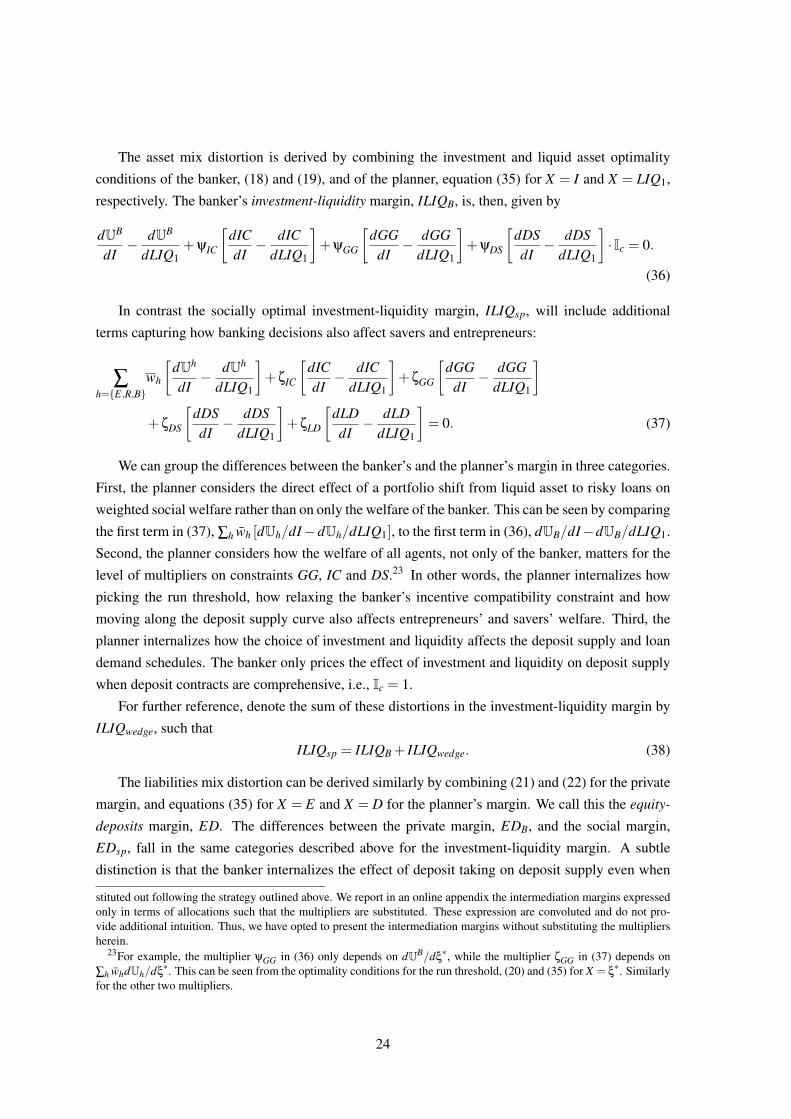
The asset mix distortion is derived by combining the investment and liquid asset optimality
conditions of the banker, (18) and (19), and of the planner, equation (35) for X = I and X = LIQ1,
respectively. The banker’s investment-liquidity margin, ILIQB, is, then, given by
dUB
dI− dUB
dLIQ1+ψIC
[dICdI− dIC
dLIQ1
]+ψGG
[dGG
dI− dGG
dLIQ1
]+ψDS
[dDSdI− dDS
dLIQ1
]· Ic = 0.
(36)
In contrast the socially optimal investment-liquidity margin, ILIQsp, will include additional
terms capturing how banking decisions also affect savers and entrepreneurs:
∑h={E,R,B}
wh
[dUh
dI− dUh
dLIQ1
]+ζIC
[dICdI− dIC
dLIQ1
]+ζGG
[dGG
dI− dGG
dLIQ1
]+ζDS
[dDSdI− dDS
dLIQ1
]+ζLD
[dLDdI− dLD
dLIQ1
]= 0. (37)
We can group the differences between the banker’s and the planner’s margin in three categories.
First, the planner considers the direct effect of a portfolio shift from liquid asset to risky loans on
weighted social welfare rather than on only the welfare of the banker. This can be seen by comparing
the first term in (37), ∑h wh [dUh/dI−dUh/dLIQ1], to the first term in (36), dUB/dI−dUB/dLIQ1.
Second, the planner considers how the welfare of all agents, not only of the banker, matters for the
level of multipliers on constraints GG, IC and DS.23 In other words, the planner internalizes how
picking the run threshold, how relaxing the banker’s incentive compatibility constraint and how
moving along the deposit supply curve also affects entrepreneurs’ and savers’ welfare. Third, the
planner internalizes how the choice of investment and liquidity affects the deposit supply and loan
demand schedules. The banker only prices the effect of investment and liquidity on deposit supply
when deposit contracts are comprehensive, i.e., Ic = 1.
For further reference, denote the sum of these distortions in the investment-liquidity margin by
ILIQwedge, such that
ILIQsp = ILIQB + ILIQwedge. (38)
The liabilities mix distortion can be derived similarly by combining (21) and (22) for the private
margin, and equations (35) for X = E and X = D for the planner’s margin. We call this the equity-
deposits margin, ED. The differences between the private margin, EDB, and the social margin,
EDsp, fall in the same categories described above for the investment-liquidity margin. A subtle
distinction is that the banker internalizes the effect of deposit taking on deposit supply even when
stituted out following the strategy outlined above. We report in an online appendix the intermediation margins expressedonly in terms of allocations such that the multipliers are substituted. These expression are convoluted and do not pro-vide additional intuition. Thus, we have opted to present the intermediation margins without substituting the multipliersherein.
23For example, the multiplier ψGG in (36) only depends on dUB/dξ∗, while the multiplier ζGG in (37) depends on
∑h whdUh/dξ∗. This can be seen from the optimality conditions for the run threshold, (20) and (35) for X = ξ
∗. Similarlyfor the other two multipliers.
24
deposit contracts are incomplete. For further reference, denote the sum of these distortions in the
equity-deposits margin by EDwedge, such that
EDsp = EDB +EDwedge. (39)
In the next section we present a numerical example of the private and planning equilibria and
discuss how the allocations differ in reference to the aforementioned intermediation margins.
3.3 Numerical example
The full set of parameters we used to solve the model is shown in Table 1. The parameterization
should be taken more as an illustrative example to highlight the mechanisms in the model rather
than as a realistic calibration of the economy attempting to make quantitative statements about the
absolute optimal level of banking regulations. We have experimented with various other parameter
choices and the findings that we emphasize are quite robust.
Our model would require some obvious modifications to use it for quantitative policy analysis.
For example, all liabilities in our model are unsecured, while in practice certain types of deposits are
insured. Deposit insurance, even partial, would reduce the market discipline exerted by depositors
and hence the credit risk premia in deposit rates bringing them closer to what is observed in reality.
Moreover, it is not clear whether the various capital regulations in practice (Basel requirements,
stress tests, restrictions on dividend payouts) are indeed binding and whether one should be cali-
brating to match a regulated economy rather than an unregulated private equilibrium. Finally, the
assumption of linearity of utilities in third period consumption, which simplifies the computation of
the run threshold significantly, as well as the finite horizon of the model make depositors willing to
accept a higher probability of a run if they were risk-averse or if there was a continuation value for
the bank. One could add convex bankruptcy costs to mimic a higher degree of risk-aversion as well
as model the continuation value, but we have not done so because it is not important to make our
fundamental analytic points.
With these caveats in mind, let us call attention to some of the considerations that we took into
account while choosing the model parameters.
First, the probabilities of default and losses given default will determine the amount of default
risk that the bank is facing. We opt to have entrepreneurs and banks default in the bad state
irrespective of the realization of the liquidation value in the intermediate period.
Second, the bank is profitable enough, and the initial equity of the banker and her preference
for current consumption are such that she voluntarily uses some of her endowment to buy more
equity in the bank. In our baseline equilibrium, the banker enjoys a positive economic surplus from
intermediating. In section 5 we examine a case that the banker has sufficient initial wealth so that
she invests in the bank up to the point that the economic surplus accruing to her is driven to zero,
i.e., she enjoys the same utility as in autarky. We believe that this is not realistic, but describing
this case is still useful to highlight that the justification for banking regulation is not to capture the
25

economic surplus of bankers, but rather to improve allocative and productive efficiency.
Third, the liquidity provision by the bank leads savers not choose to additionally self-insure
by holding the liquid asset. When savers self-insure, the banking sector is under-performing as a
provider of liquidity and, hence, intermediation, and regulations that make banks more stable would
have an additional positive effect. In our baseline parameterization we want to mute this channel
and make it harder for regulation to improve economic outcomes. However, our results hold even
when savers self-insure in the private equilibrium.
Fourth, we have chosen the parameters, among them, most importantly, the liquidity preference
shock, the distribution of the liquidation value and risky technology payoffs, such that the bank
holds a portfolio of both liquid assets and risky loans, and also liquidates part of its risky holdings
to serve early withdrawals.
Fifth, we have chosen logarithmic utility for period 1 and period 2 consumption, while we spe-
cialize the production function to be F =(I + IE)α
`1−α =(I + IE)α
, with α< 1 and entrepreneurial
skills’ supply normalized to `= 1.24
Before presenting the model solution and explaining how the private and social equilibria differ,
we briefly describe some regulatory ratios and risk metrics that we have constructed to facilitate the
analysis.
The capital adequacy ratio (CR) is equal to the value of equity divided by the level of risky
loans. We have normalized the risk-weight on loans to one, while liquid assets receive a risk-weight
of zero:
CR =EI. (40)
The leverage ratio (LevR) includes both the risky and liquid holdings and is given by:
LevR =E
I +LIQ1. (41)
The liquidity coverage ratio takes the (lowest) liquidation value of the bank’s portfolio in a run
relative to runnable liabilities:25
LCR =LIQ1 +ξ · ID ·(1+ rD
2
) . (42)
Finally, we compute a net stable funding ratio which is computed as the fraction illiquid assets
24The original Diamond-Dybvig framework requires the relative risk-aversion coefficient to be higher than one. Thisis not necessary when the liquidation value of long-term investment can be lower than one as pointed out by Cooper andRoss (1998). In addition, the share of income for the risky technology accruing to entrepreneurial human capital (setto 0.25) is chosen to reflect estimates from the literature. Gollin (2005) finds that the share of profits in entrepreneurialactivities is 0.10. The rest is the share of labor and capital. In our setting, labor from workers is not modeled, and we areinterested in the share of the remaining output which is distributed to entrepreneurs and suppliers of capital. Setting theshare of capital relatively to labor to 0.30, which is standard in the literature, give a relative share for entrepreneurial andcapital profits of 0.1/(0.1+0.9 ·0.3) = 0.28 and (0.9 ·0.3)/(0.1+0.9 ·0.3) = 0.72, respectively.
25It is not obvious whether to count the portion of the loans that are always available as being liquid or not. Our resultsare very similar if we exclude them from the numerator of this regulation.
26
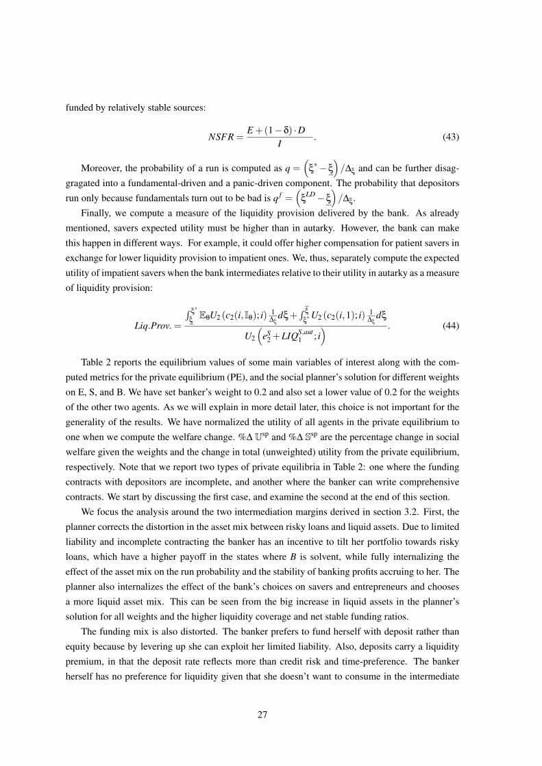
funded by relatively stable sources:
NSFR =E +(1−δ) ·D
I. (43)
Moreover, the probability of a run is computed as q =(
ξ∗−ξ
)/∆ξ and can be further disag-
gragated into a fundamental-driven and a panic-driven component. The probability that depositors
run only because fundamentals turn out to be bad is q f =(
ξLD−ξ
)/∆ξ.
Finally, we compute a measure of the liquidity provision delivered by the bank. As already
mentioned, savers expected utility must be higher than in autarky. However, the bank can make
this happen in different ways. For example, it could offer higher compensation for patient savers in
exchange for lower liquidity provision to impatient ones. We, thus, separately compute the expected
utility of impatient savers when the bank intermediates relative to their utility in autarky as a measure
of liquidity provision:
Liq.Prov.=
∫ ξ∗
ξEθU2 (c2(i,Iθ); i) 1
∆ξ
dξ+∫ ξ
ξ∗U2 (c2(i,1); i) 1
∆ξ
dξ
U2
(eS
2 +LIQS,aut1 ; i
) . (44)
Table 2 reports the equilibrium values of some main variables of interest along with the com-
puted metrics for the private equilibrium (PE), and the social planner’s solution for different weights
on E, S, and B. We have set banker’s weight to 0.2 and also set a lower value of 0.2 for the weights
of the other two agents. As we will explain in more detail later, this choice is not important for the
generality of the results. We have normalized the utility of all agents in the private equilibrium to
one when we compute the welfare change. %∆ Usp and %∆ Ssp are the percentage change in social
welfare given the weights and the change in total (unweighted) utility from the private equilibrium,
respectively. Note that we report two types of private equilibria in Table 2: one where the funding
contracts with depositors are incomplete, and another where the banker can write comprehensive
contracts. We start by discussing the first case, and examine the second at the end of this section.
We focus the analysis around the two intermediation margins derived in section 3.2. First, the
planner corrects the distortion in the asset mix between risky loans and liquid assets. Due to limited
liability and incomplete contracting the banker has an incentive to tilt her portfolio towards risky
loans, which have a higher payoff in the states where B is solvent, while fully internalizing the
effect of the asset mix on the run probability and the stability of banking profits accruing to her. The
planner also internalizes the effect of the bank’s choices on savers and entrepreneurs and chooses
a more liquid asset mix. This can be seen from the big increase in liquid assets in the planner’s
solution for all weights and the higher liquidity coverage and net stable funding ratios.
The funding mix is also distorted. The banker prefers to fund herself with deposit rather than
equity because by levering up she can exploit her limited liability. Also, deposits carry a liquidity
premium, in that the deposit rate reflects more than credit risk and time-preference. The banker
herself has no preference for liquidity given that she doesn’t want to consume in the intermediate
27

period and would like to extract any liquidity premium by using deposit funding. The planner
instead prefers more equity funding and a more stable capital structure. Hence, the planner chooses
higher common equity and higher capital adequacy. By doing so, the planner’s allocations allow the
bank to operate with a larger balance sheet. Despite a higher capital ratio, the bank operates with a
lower leverage ratio and delivers its intermediation services more efficiently.
The more stable asset and funding choices of the planner come from the desire to reduce run
risk. The probability that a run occurs drops in the planner’s solution, as does the probability of fun-
damental runs. Overall, this improves the stability of the banking sector and enhances the stability
of real economic activity as the entrepreneur sees her funding being withdrawn less frequently.26
Moreover, the planner reduces maturity transformation in relative terms, which can be seen by
the higher risk weighted capital and net stable funding ratios. However, the reduction in maturity
transformation is not necessarily accompanied by a drop in the level of credit extension. For suffi-
ciently high wE , the planner chooses higher investment than in the private equilibrium. Indeed, we
show that increasing the equity in the bank, without requiring more liquidity, leads to more credit
extension through a combination of channels described in detail in sections 4.1 and 4.2 where we
study capital and leverage requirements in isolation. On the contrary, credit extension is lower when
the saver is favored and the planner forces the bank to hold more liquid assets. Overall, private allo-
cations can exhibit both under- and over-investment indicating that the source of inefficiency is not
the total level of lending, but its relation to the holding of liquid assets and the funding structure of
the bank.
Liquidity provision is also higher in the planner’s solution. In fact, liquidity provision as mea-
sured in (44) is below one in the private equilibrium, which suggests that the banker offers attractive
enough returns to patient depositors to induce them to accept lower utility when they turn out to
be impatient – the deposit terms still deliver higher overall utility than in autarky. This may not be
surprising given that the banker favors lending over holding liquidity, so the bank finds it more dif-
ficult to provide insurance to impatient savers. Instead the planner delivers more liquidity provision
to impatient depositors without sacrificing long-term returns to patient savers.27 This is possible
because the planner’s choices lead to a larger overall level of intermediation.
The enhanced stability of both the asset portfolio and capital structure of the bank are beneficial
26The fact that panic-driven runs occur with non-negligible probability suggests that government guarantees, such asdeposit insurance or implicit bailout subsidies, may be useful policy interventions. We have abstracted from introducinggovernment guarantees in the model for two reasons. First, it would not unambiguously improve outcomes as in theoriginal Diamond-Dybvig set-up because of risk-taking incentives (see, for example, Kareken and Wallace, 1978, Cooperand Ross, 2002, Admati et al., 2012). Second, designing deposit insurance when runs have both a fundamental andpanic risk component is far from straightforward. Such an exercise is not trivial and is beyond the scope of the currentpaper which aims to identify the banking externalities arising from incomplete contracting for credit and run risk (Allenet al., 2015, study government guarantees within a global games framework and a simpler banking sector that the one inour paper). In the same token, we do not study emergency liquidity assistance from a Lender of Last Resort (Rochet andVives, 2004) or suspension of convertibility (Ennis and Keister, 2009), which would also require non-trivial modificationsin the model we present. See also Keister (2015) for an analysis of efficient bailouts, which should be complemented withprudential regulation. We believe that these are important avenues for future research in models that feature an elaboratebanking sector subject to both credit and run risk like ours.
27Though not shown in the table, the utility of the patient savers is higher than in the private equilibrium.
28

to savers and entrepreneurs. However, the banker is worse-off; in our model the banker internalizes
all the effects that matter for her welfare and optimally chooses more risk to maximize her own
utility. The planner cares about the externalities to the other agents as well and weakens the ability
of the banker to take advantage of her limited liability. In fact, the banker’s welfare always drops
in the planner’s solutions and drives the banker to her participation constraint, unless the weight
on the banker is (unreasonably) high. We do not explore such planning equilibria because they
cannot be implemented with banking regulation, which always drives bankers utility down, as it
will become more clear in section 4. Nevertheless, the planner not only increases social welfare
(Usp), which depends on Pareto weights, but also the overall surplus in the economy, which is
captured by the change in Ssp. The planner could improve the welfare all agents if she had access
to a re-distributive, non-distortionary (lump-sum), tax system to transfer resources across agents. In
section 5, we examine equilibria where a very wealthy banker injects enough equity into the bank to
drive the economic profits to zero. In this case, we show that a Pareto improvement over the private
equilibrium is possible.
Finally, the planner chooses different levels of capital and liquidity depending on which agents
she favors most. When the weight on the entrepreneur is higher, the planner chooses more capital
to support higher lending. This is beneficial for the entrepreneur, but results in lower liquidity
provision, which is relatively bad for savers. On the contrary, when the weight on savers is higher,
the planner chooses a more liquid asset mix.
We should note that neither the banker nor the planner hold excess liquidity, i.e., LIQ2(ξ,δ) = 0
for all ξ. Holding excess liquidity could be desirable in order to eliminate the probability of a
run altogether. If the liquidation value of the bank for the lowest possible realization of ξ was
higher that the total runnable deposit obligations, i.e., LIQ1 +ξ · I ≥D(1+ rD2 ), then only impatient
depositors would withdraw. The excess liquidity carried over to period 3 would then be LIQ2 =
LIQ1− δ ·D(1+ rD2 ) ≥ (1− δ)D(1+ rD
2 )− ξ · I. Such run-proof equilibria may not be desirable
when the lowest liquidation value of long-term investment is small or when savers are not very
risk-averse. A fair amount of literature has focused on run-proof equilibria, which naturally restrict
credit intermediation (see Cooper and Ross, 1998, Ennis and Keister, 2006, Diamond and Kashyap.
2016). Run-proof contracts require certain assumptions to be optimal and our work has, instead,
focused on optimal policy in the presence of both run risk and credit risk.
Before turning to the implementation of the planning outcomes, we discuss the private equilib-
rium when deposit contracts are comprehensive, i.e., Ic = 1 in the banker’s optimization conditions.
The results are reported in the third column in Table 2. Comprehensive deposit contracts allow the
banker to commit, but she still chooses the levels of risk that improves her own utility and does not
internalize all the effects on other agents. Acting in her own interests, the banker still chooses a
riskier asset and liabilities structure than a planner would. The social planner instead internalizes
the effects of all decisions on all agents utility, and choose a less risky asset mix and liabilities
structure. The gap between the social and private equilibrium grows with commitment, because in
this case the banker offers a contract that is even more skewed towards her interests at the expense
29
of the other agents. Indeed, as the table shows the banker’s choices result in lower welfare for en-
trepreneurs and savers compared to the private equilibrium with incomplete deposit contract, and
the participation constraint of savers starts binding.
4 Regulation
We now explore how the planner’s solution can be decentralizing via various regulatory interven-
tions, which tighten the regulatory ratios (40)-(43). Sections 4.1-4.4 discuss the effects when the
tools are used in isolation. Section 4.5 discusses how the regulations can be optimally combined to
implement the planner’s solution as a private equilibrium. Table 3 reports the results for the various
regulations.
4.1 Capital Requirements
Capital regulation requires the bank to hold a certain percentage of equity for every unit of risky
loans extended and it formally amounts to increasing CR in equation (40).
Mandating higher capital requirements reduces the ability of the banker to take risk through de-
posit funding. In models where the bank cannot raise additional equity, stricter capital requirements
(mechanically) result in a drop in credit extension (see, for example, Corbae and D’Erasmo, 2014,
Clerc et al. 2015 and the references therein). More generally, one could allow banks to raise both
equity and deposits. Then, capital regulation has an effect if the Modigliani-Miller theorem is vio-
lated. Despite abstracting from any tax advantages of debt, which is the most common violation put
forward, our environment breaks Modigliani-Miller in various ways, even holding the probability
that a run occurs constant. First, deposits carry a liquidity premium.28 Second, the available equity
capital is not perfectly elastically supplied and, from (21), the banker requires a higher return if she
contributes more equity. Third, default is costly and there are positive bankruptcy costs. The first
two frictions push for higher cost of funding, while the last for lower, when capital requirements
increase. Although the overall partial equilibrium effect, fixing the probability of a run and the
liquidity premium, seems ambiguous, it is plausible to suppose that the three forces result in higher
funding costs and lower lending for low enough bankruptcy costs.
But our model features additional channels which push up lending. The first important channel
is that higher capital reduces the probability of a run. This makes savers more willing to make
deposits and the entrepreneurs more inclined to borrow.29 Second, substituting equity financing
for deposit financing on the margin allows the bank to hold less liquidity to serve the impatient
households. This would incrementally free up resources to be invested in risky loans. Finally, the
28See Van den Heuvel (2008) and Hanson, Kashyap and Stein (2011) for estimates of the liquidity premium for bankdeposits.
29In a model where the bank is funded only with deposits, Ennis and Keister (2006) show that shifting the assetmix towards more illiquid loans would result in a lower probability of being repaid given that a run occurs, whichcounterbalances the increase in credit extension when the probability of a run decreases. This does not need to be true inour model, because the increase in the credit extension is funded by more capital.
30

reduced demand for deposits suppresses incrementally the deposit rate, other things equal, due to
impatient savers’ liquidity demand.30
Accounting for all these considerations, lending rises when capital requirements increase.31
There are other noteworthy general equilibrium effects that also arise. For example, the cost of
funding decreases which also allows for lower loan rates.32 Moreover, the lower probability of a
run allows for more deposit taking, which pushes the deposit rate up; the banker continues to try
to take advantage of her limited liability and funding higher investment exclusively with equity is
expensive. Finally, capital requirements do not necessarily need to result in lower liquidity holdings.
The opportunity cost of liquidating risky loans increases because the loans are funded with a more
expensive source of financing on the margin. Hence, the bank chooses to liquidate a smaller portion
of its loan portfolio in the intermediate period for any realization of the liquidation value (though this
is not shown in Table 3). This result is why the holdings of liquid assets also increase with higher
capital requirements, but the bank still holds less liquidity that the planner would. This implies that
capital and liquidity regulation could be optimally combined as we show in section 4.5.
Although credit extension goes up, the regulation has two important implications. First, the
higher credit extension needs to be funded exclusively with more equity. Second, liquid asset
holdings also rise. As we will discuss in the following section, this is not the case under the
risk-insensitive leverage regulation, because that type of rule allows the banker to offset lending
increases with reductions in liquid assets.
On net, run risk falls because the bank uses a lower percentage of deposit funding. The reduction
in run risk is beneficial for savers and entrepreneurs. The level of deposits need not fall, because the
bank is safer overall and hence its total balance sheet grows. This mean that liquidity provision can
be maintained. However, the banker is made worse-off with higher capital requirements, which is
not surprising given that she could have voluntarily chosen more capital if it was beneficial for her.
Of note, the level of capital requirements that maximizes social gains without violating bankers’
participation constraints, is higher than the capital ratio in the planner’s solution. As we discuss in
section 4.5, the planner uses multiple tools to implement the socially optimal allocations. If a
regulator is limited to one tool, that tool must be used more aggressively than if several can be
deployed, so it’s value will “over-shoot” the level that a planner will pick. As we see below, this is
true for all the tools.30Begenau (2015) also shows in a real business cycle framework that the fall in the deposit rate, when capital require-
ments increase and savers value the liquidity services of deposits, can push the overall cost of funding down and result inhigher credit extension. The strength of this mechanism is mitigated when savers can also purchase bank equity (see theextended model in the online appendix).
31We have experimented with several versions of the model and parameterizations and this conclusion is very robust.32The first order condition with respect to E, (21), becomes ψBS = γ ·U ′(eB−E)−ψCR. Although more equity pushes
the cost of funding up, as measured by the bankers marginal utility, the Lagrange multiplier on the capital requirement,ψCR, operates in the opposite direction and in equilibrium it dominates.
31

4.2 Leverage Requirements
Leverage regulation ties the level of capital to the overall size of the bank’s balance sheet and it
formally amounts to decreasing LevR in equation ( 41).
Leverage requirements operate through the same channels as capital requirements, i.e., they
reduce the ability of the banker to take risk through deposit funding. Overall, they push credit
extension up, but there is a critical difference. Risk-weighted capital regulation requires banks to
hold more capital only against risky loans, while leverage regulation mandates more capital against
all assets and, hence, it does not directly affect the marginal choice between investment and liquidity.
Although the banker is required to operate with a safer liability structure, she can tilt the asset mix to
reduce liquid assets and raise lending. As a result, credit extension should increase relatively more
from tightening the leverage requirements than from raising risk-weighted capital requirements.
The increase in asset illiquidity increases fundamental run risk. The drop in liquid holdings and
lower demand for deposits makes savers worse-off, who are pushed to their participation constraint
for small changes in the regulation. Entrepreneurs are marginally better-off due to the higher credit
extension, but the drop in social welfare suggests that leverage requirements would not be used in
isolation in this economy. This conclusion is not robust to some reasonable modifications of the
environment – see for example the extension in the online appendix. However, even in the model as
it stands, below we show that leverage regulation can be combined with other regulations to improve
economic outcomes. As with all the regulations we consider, the banker is worse-off.
4.3 Liquidity Requirements
A liquidity-coverage-ratio regulation requires that the immediately available funding for the bank
is at least a certain percentage of runnable debt (deposits) and, in our model, it formally amounts to
increasing LCR in equation (42).33
Mandating that the bank holds more liquidity changes the trade-off between investing in risky
loans and liquid assets, since liquid assets count fully towards this regulation and loans do not.
Looked at in isolation, this regulation reduces the incentive to fund loans through deposits.
Liquidity requirements are good tools for raising liquidity and reducing credit extension. How-
ever, they erode bank profitability and make it harder to raise equity. The amount of equity falls
as does the capital adequacy ratio (despite the decrease in credit extension). The bank switches to
more deposit financing to compensate for lower equity financing and leverage is higher than both
the PE and SP outcomes. Overall this regulation has the ability to reduce risk on the asset side, but
it results in higher risk on the liability side.34
33We focus on a form of liquidity coverage regulation, but the results in this section hold more generally for othertypes of liquidity regulation, such simple restrictions on the ratio of liquid to illiquid assets (LIQ1/I) or reserve ratiorequirements (LIQ1/D).
34The literature has studied additional market failures that justify the regulation of banks’ liquidity. In Allen and Gale(2004) and Diamond and Rajan (2011) the need for policy intervention stems from the presence of fire-sales, in Farhi,Golosov and Tsyvinski (2009) liquidity regulation tackles inefficient risk-sharing due to hidden trades, while Diamondand Kashyap (2016) show that liquidity requirements are important to deter run risk when depositors have incomplete
32

However, the lower probability of runs is beneficial to both savers and entrepreneurs, and the
high level of deposits improves liquidity provision. Yet, the decrease in credit extension results
in higher benefits for savers than for entrepreneurs compared to the planner’s solution, while the
opposite hold for capital and leverage regulations. Finally, the banker sees her welfare going down
for the same reason described before.
4.4 Net Stable Funding Requirements
This type of regulation requires that the bank funds a certain percentage of illiquid assets with long-
term, stable sources of financing, which in our model are equity and the portion of deposits that will
not be withdrawn. Formally, the regulation sets a higher value for NSFR in equation (43).
The effects of NSFR regulation are parallel to the LCR. Investment goes down, liquidity im-
proves, and the bank relies more on deposit funding rather than equity capital. Similarly, the proba-
bility of bank runs goes down.
A generalized version of the NSFR could be calibrated to look more like capital or liquidity
regulation. Suppose that the relative weights on equity capital and stable deposits that appear in
the numerator of the NSFR could vary. Figure 1 shows the change in credit extension for this
generalized version of the net stable funding ratio where equity and long-term deposit funding are
weighted differently, i.e., NSFR = (E +w · (1−δ) ·D)/I with 0 < w≤ 1. Depending on the weight
on deposits, an increase in the NSFR would resemble more closely the effects of capital versus
liquidity regulations. In particular for a low weight on deposits, the NSFR results in higher credit
extension similarly to capital requirements, while for higher weights credit extension decreases
similarly to liquidity requirements.
4.5 Optimal Regulatory Mix
This section examines whether and how regulation can be combined to implement the social plan-
ner’s solution as a private equilibrium. The social planner solves for allocations without taking into
consideration how the optimal behavior of the bank will change, or in other words the first-order
conditions of the banker (adjusted for regulatory interventions) are not taken as additional con-
straints in (34) – though the banker’s participation constraint must be satisfied. Hence, the planner’s
allocations are computed without tying the planner to specific tools. This way we have been able to
clearly identify the distorted margins between the privately and socially optimal decisions in section
3.2. The rest of the section shows how the regulatory tools studied above can be combined to correct
for the distorted banking decisions derived as the wedges in conditions (38) and (39).
For that purpose we set-up an augmented planner endowed with certain regulatory tools. Let Tbe the available set of regulatory tools which will include at least the four regulations studied above
and possibly others. For each T ∈ T there is a regulatory constraint RC(T,X) ≥ 0, which ties the
tool with the endogenous variables X ∈ X (for example, constraints (40)-(43)). It is important to
information about banks’ asset portfolios. Finally, Calomiris, Heider and Hoerova (2015) discuss how liquidity regulationcan provide the right incentives for managing risks under deposit insurance guarantees.
33

note that the regulatory constraints are defined as inequalities, i.e., the planner can tighten them,
but not loosen them. Let ψT be the multipliers that the banker in the private equilibrium assigns to
constraint RC(T,X)≥ 0.
Under regulation, the optimization margins change to:
ILIQT : ILIQB +∑T
ψT
[dRC(T,X)
dI− dRC(T,X)
dLIQ1AILIQ +
dRC(T,X)
dE(1−AILIQ)
]= 0, (45)
EDT : EDB +∑T
ψT
[dRC(T,X)
dE(1+AED)−
dRC(T,X)
dD+
dRC(T,X)
dIAED
]= 0, (46)
where AILIQ and AED are given by (A.9) and (A.11) in the online appendix.
The tools-augmented planner’s problem, akin to a Ramsey planner’s problem in the public fi-
nance literature (see, for example, Lucas and Stokey, 1983), is derived in an online appendix.35 To
implement the equilibrium allocations of the social planner, denoted by X sp, the available tools, T ,
have to be chosen such that, first, X sp satisfy the regulatory constraints RC(T,X sp) = 0, and, second,
the intermediation margins in the associated equilibrium are the same as the intermediation margins
of the planner. Essentially, this means that the additional terms in (45) and (46) need to equal the
wedges derived in (38) and (39). In matrix form, this can be written as:
∆RC ·Ψ =WDsp, (47)
where Ψ is the Tx1 vector of the multiplier on the T regulatory constraints, WDsp is the 2x1 vector
of the wedges in the two intermediation margins evaluated at the planner’s equilibrium values, and
∆RC is the 2xT matrix of the partial derivatives of the relevant variables for each intermediation
margin on the T regulatory constraints. These derivatives are also evaluated at the equibrium values
for the variables X sp and for the levels of the tools T sp, which implicitly solve RC(T sp,X sp) = 0.
Hence, it suffices to find two regulatory tools such, first, the matrix ∆RC is invertible, and,
second, all elements in Ψ are positive. We will now explain these conditions in more detail and
provide the underlying economic intuition.
Given that the banks’ asset and liability mix are each distorted, two tools are generally needed
to implement the planner’s allocations. The exception would be if the distortions turn out to alter
both mixes in identical ways. In this, measure zero, case the wedges would be “equal” to each other
in equilibrium. Moreover, the optimization variables should not load on the regulatory constraints
in a collinear way, or, in other words, the matrix ∆RCsp should not be singular. This means that
the choice of one tool should not determine the level of another tool and, hence, there are enough
degrees of freedom to correct both of the distortions.
35The problem in the Ramsey literature is to maximize a social welfare function subject to all the constraints constitut-ing a competitive equilibrium for the purpose of financing government expenditure with distortionary taxation. Althoughthe purpose of our augmented planner is different, the methodology to optimally choose the level of instruments that sheis endowed with is the same.
34

Finally, the regulatory tools should be jointly binding, which means that the multipliers ψT
should be strictly positive. The reason is that quantity regulations as in (40)-(43) mandate a min-
imum level of capital, liquidity or combinations of assets and liabilities, and the bank cannot be
forced to operate at a lower level. This becomes important when tools, which are binding by them-
selves in the private equilibrium, are combined.
In order to examine which regulations can be jointly binding, we set the level of tools to the
regulatory ratios in the planner’s solution and compute the vector of multipliers Ψ for all possible
combinations. It turns out that many pairs of regulations can be combined to deliver the planner’s
allocations. As long as one of the pair is a capital tool (CR or LevR) and the other a liquidity
tool (LCR or NSFR) then the regulations will replicate the planner’s allocations. This result is
intuitive. The planner wants to hold more liquidity and more capital than in the private equilibrium.
Liquidity requirements can force more liquidity in the bank, but at the cost of reducing capital ratios
or, equivalently, increasing leverage. Hence adding a capital or leverage requirement can correct
for the (unintended) consequences of liquidity regulation. Yet, two liquidity tools cannot be jointly
binding as they reinforce each other and move the key variables in the same direction.36 The same
problem arises if only the two capital regulations are deployed. Otherwise, the palnner’s outcome
shown in the last column of Table 3 can be delivered by any of the four combinations of that involve
a single capital regulation along with a single liquidity regulation.
5 Social outcomes, regulation and banker’s wealth abundance
Until now, our analysis has focused on equilibria where banking is sufficiently profitable for the
banker, i.e., her utility is above her reservation value. We have shown that regulation depletes
this surplus, but improves economic efficiency and increases the total surplus created. This raises
the question of whether regulation is needed just because the banker, acting in her own interests,
maximizes the surplus accruing to her. Although regulation has redistributive aspects, we show in
this section that it is beneficial even when the banker is receives zero economic surplus in the private
equilibrium.
One way to clarify these issues is to consider a banker who is wealthy enough that the marginal
value of consumption at t=1 (or the relevant outside option in a richer model) is sufficiently low.
In this case, the banker will invest in so much bank equity that the banker’s participation constraint
is binding in the private equilibrium. Table 4 reports the private and planning outcomes for two
levels of the bankruptcy cost. As we discuss below, the level of the bankruptcy cost is not important
36Our results are consistent with the analysis in Checchetti and Kashyap (2016), who show that LCR and NSFRregulations almost surely will never bind at the same time. However, the collinearity of the CR and LevR regulationsmay be specific to our model. If the bank that could choose between more types of assets with different levels of risk,or to hold off-balance sheet assets, this result may no have obtained – though this would not likely deliver the planner’sallocations. Although we can only speculate at this point, we believe that such modifications are important avenuesfor future research. Other papers that study the use of capital and liquidity requirements include Walther (2016) andKara and Ozsoy (2016) in the presence of fire sale externalities, Boissay and Collard (2016) when the interbank marketcannot efficiently allocate resources, and Van den Heuvel (2017) who quantifies the welfare costs of capital and liquidityrequirements in a neoclassical growth model.
35

to obtain divergent private and social outcomes, but matters for the kind of regulation that can
decentralize the planner’s solution.
As in the general case when the banker’s utility exceeds her reservation value, the planner con-
tinues to favor a lower run probability. Social welfare improves and the total surplus is higher than
in the private equilibrium. Moreover, Pareto improvements are possible, whereby both savers and
entrepreneurs are better-off compared to the private equilibrium. Nevertheless, the choice of the
asset mix and of the liabilities structure depends on the agent who is favored more and the level
of deadweight losses in bankruptcy. The tensions arise because in this equilibrium the banker can-
not simultaneously increase both capital and liquidity. The banker is already at her participation
constraint in the private equilibrium, asking her to contribute more equity requires a reduction in
liquidity so the lower return to equity is counterbalanced by the positive effect of holding fewer
liquid assets (and vice versa). The planner cannot require both higher capital and liquidity without
violating the banker’s participation constraint.
If bankruptcy costs are low, the risk-sharing effect of higher capital is less strong and the planner
chooses more liquid assets. As a result, investment goes down and savers enjoy most of the gains
from the intervention, while entrepreneurs are slightly better-off for most weights and worse-off for
low wE . In this case, planning outcomes can be fully decentralized with just one liquidity regulation.
If bankruptcy costs are high, raising capital requirements is a more efficient way to improve
social welfare and investment goes up. This outcome is equally beneficial for entrepreneurs and
savers. Finally, planning outcomes can be fully decentralized with just one capital tool.
For all of the prior results, where the banker enjoys positive economic surplus in the private
equilibrium, both a capital tool and a liquidity tool are needed for decentralization irrespective of
the level of the bankruptcy cost.
6 Conclusions
Banks perform important services for the real economy using both sides of their balance sheet.
However, the private banking equilibria may not be socially optimal and regulating banking activi-
ties can improve social welfare. We have examined how many regulations that are often discussed in
policy discussions perform in a relatively familiar model of banking. We started from the Diamond
and Dybvig (1983) benchmark precisely because it is so thoroughly studied. The modifications
that we made trade-off tractability to keep the model relatively simple, against our preference for
additional realistic forces that the baseline model excludes.
Our modifications generate endogenous credit risk in banks’ portfolios as well as the risk of an
endogenous funding run. This simple pair of features interact in interesting and unexpected ways.
We draw several general lessons from the model that we believe will carry over to many other
models.
First, we identify two general intermediation margins that are distorted, i.e., the relative amounts
of liquid and illiquid assets and the mix of deposits and equity. The way that banks privately set
36

these margins diverges from what a social planner would choose, because bankers do not fully
internalize the effects of their choices on savers and entrepreneurs. In particular, a social planner
chooses relatively more liquidity and equity than the banker. As a result, the planner reduces run
risk, improves the provision of liquidity, and guarantees a more stable extension of credit and real
production compared to the private equilibrium. These two distortions will be present if we expand
the set of assets that banks can invest in or the types of funding sources, but additional ones may
also arise.
Second, the two wedges between the private and social choices are not collinear. Thus, more
that one regulatory tool is needed to implement the socially optimal allocations. Optimal policy
in models without both distortions can be misleading. For example, if the liability structure is
constrained, say because deposit levels are exogenously determined and equity is fixed, studying
asset allocations and distortions becomes much easier. But, regulation, if any is needed, will amount
to fixing liquidity ratios. Similarly, shutting down the liquidity demand and liquidity risk makes it
easier to focus on the optimal capital structure and level of investment. But, regulation, if again
any is needed, would amount to fixing capital ratios. Instead, when both sides of the bank’s balance
sheet are endogenously determined the distortions from each side interact and a combination of both
capital and liquidity requirements emerge in the optimal regulatory mix.
Third, the political economy aspects of regulation deserve attention. Our bankers internalize
how their decisions matter for run risk and choose funding contracts optimally to maximize their
own welfare. Their distorted choices, from a social point of view, have real macroeconomic con-
sequences. Regulation improves aggregate welfare, but reduces the rents accruing to bankers. If
possible, therefore, banks’ incentives to engage in regulatory arbitrage would be strong. The lack
of regulatory arbitrage in the model we have studied is one of its main shortcomings. Moreover,
regulating capital and/or liquidity is beneficial for both savers and entrepreneurs, but the relative
benefits of the type of regulation differ. Savers gain more with liquidity regulation given that it has
a bigger effect of liquidity provision, while entrepreneurs gain more with capital regulation given
that it allows for more credit extension.
There are other interesting avenues to extend our model, some of which we have already been
mentioned and are analyzed in the online appendix. One further direction would be to allow banks to
issue long-term debt together with demandable deposits and equity. Including loss-absorbing debt
instruments in the regulatory mix could introduce additional ways to tackle with run risk and credit
risk. But it would not constitute a full remedy by itself due to the disciplinary role that demandable
liabilities play. Moreover, our model is flexible enough to incorporate fire-sale dynamics by endo-
genizing the liquidation value of long-term investment. Although this would introduce pecuniary
externalities as an additional reason why private allocations are inefficient, it would not qualitatively
overturn our main conclusions; the asset and liability side distortions would be similar. Finally, one
could enrich the set of risky investments from which a banker could choose and, thus, increase the
scope for asset substitution. Setting the (relative) risk-weights in capital requirements to capture
social risks would be, then, highly important.
37

References
Admati, A.R., P.M. Demarzo, M.F. Hellwig and P.C. Pfleiderer (2012), ‘Debt overhang and capitalregulation’, Rock Center for Corporate Governance at Stanford University Working PaperNo.114 .
Allen, Franklin and Douglas Gale (1997), ‘Financial markets, intermediaries, and intertemporalsmoothing’, Journal of Political Economy 105(3), 523–546.
Allen, Franklin and Douglas Gale (1998), ‘Optimal financial crises’, Journal of Finance53(4), 1245–1284.
Allen, Franklin and Douglas Gale (2004), ‘Financial intermediaries and markets’, Econometrica72(4), 1023–1061.
Allen, Franklin, Elena Carletti, Itay Goldstein and Agnese Leonello (2015), ‘Government guaran-tees and financial stability’, working paper .
Allen, Franklin, Elena Carletti and Robert Marquez (2015), ‘Deposits and bank capital structure’,Journal of Financial Economics 118(3), 601–619.
Angeloni, I. and E. Faia (2013), ‘Capital regulation and monetary policy with fragile banks’, Journalof Monetary Economics 60(3), 311–324.
Begenau, Juliane (2015), ‘Capital requirements, risk choice, and liquidity provision in a businesscycle model’, Harvard Business School, working paper 15-072 .
Benston, G.J. and C.W. Smith (1976), ‘A transactions cost approach to the theory of financial inter-mediation’, Journal of Finance 31(2), 215–231.
Bianchi, Javier and Enrique C. Mendoza (forthcoming), ‘Optimal time-consistent macroprudentialpolicy’, Journal of Political Economy .
Boissay, Frédéric and Fabrice Collard (2016), ‘Macroeconomics of bank capital and liquidity regu-lations’, BIS Working Papers No 596 .
Boissay, Frédéric, Fabrice Collard and Frank Smets (2016), ‘Booms and banking crises’, Journal ofPolitical Economy 124(2), 489–538.
Boyd, John H. and Gianni De Nicoló (2005), ‘The theory of bank risk taking and competitionrevisited’, Journal of Finance 60(3), 1329–1343.
Calomiris, Charles W. and Charles M. Kahn (1991), ‘The role of demandable debt in structuringoptimal banking arrangements’, American Economic Review 81(3), 497–513.
Calomiris, Charles W., Florian Heider and Marie Hoerova (2015), ‘A theory of bank liquidity re-quirements’, mimeo .
Chari, V.V. and R. Jagannathan (1988), ‘Banking panics, information, and rational expectationsequilibrium’, Journal of Finance 43(3), 749–761.
Checchetti, Stephen G. and Anil K Kashyap (2016), ‘What binds? Interactions between bank capitaland liquidity regulations’, in The Changing Fortunes of Central Banking, edited by PhilippHartmann, Haizhou Huang, Dirk Schoenmaker .
Choi, Dong Beom, Thomas M. Eisenbach and Tanju Yorulmazer (2016), ‘Sooner or later: Timingof monetary policy with heterogeneous risk-taking’, American Economic Review: Papers &Proceedings 106(5), 490–495.
38
Clerc, Laurent, Alexis Derviz, Caterina Mendicino, Stephane Moyen, Kalin Nikolov, Livio Stracca,Javier Suarez and Alexandros P. Vardoulakis (2015), ‘Capital regulation in a macroeconomicmodel with three layers of default’, International Journal of Central Banking 11(3), 9–63.
Cooper, R. and T.W. Ross (1998), ‘Bank runs: Liquidity costs and investment distortions’, Journalof Monetary Economics 41(1), 27–38.
Cooper, R. and T.W. Ross (2002), ‘Bank runs: Deposit insurance and capital requirements’, Inter-national Economic Review 43(1), 55–72.
Corbae, Dean and Pablo D’Erasmo (2014), ‘Capital requirements in a quantitative model of bankingindustry dynamics’, working paper .
Dewatripont, Mathias and Jean Tirole (1994), ‘The prudential regulation of banks’, MIT press .
Diamond, Douglas W. (1984), ‘Financial intermediation and delegated monitoring’, Review of Eco-nomic Studies 51(3), 393–414.
Diamond, Douglas W. and Anil K Kashyap (2016), ‘Liquidity requirements, liquidity choice andfinancial stability’, NBER Working Papers 22053 .
Diamond, Douglas W. and Philip H. Dybvig (1983), ‘Bank runs, deposit insurance, and liquidity’,Journal of Political Economy 91(3), 401–419.
Diamond, Douglas W. and Raghuram G. Rajan (2000), ‘A theory of bank capital’, Journal of Fi-nance 55(6), 2431–2465.
Diamond, Douglas W. and Raghuram G. Rajan (2001), ‘Liquidity risk, liquidity creation, and finan-cial fragility: A theory of banking’, Journal of Political Economy 109(2), 287–327.
Diamond, Douglas W. and Raghuram G. Rajan (2011), ‘Fear of fire sales, illiquidity seeking, andcredit freezes’, Quarterly Journal of Economics 127(2), 557–591.
Ennis, Huberto M. and Todd Keister (2005), ‘Optimal fiscal policy under multiple equilibria’, Jour-nal of Monetary Economics 52(8), 1359–1377.
Ennis, Huberto M. and Todd Keister (2006), ‘Bank runs and investment decisions revisited’, Journalof Monetary Economics 53(2), 217–232.
Ennis, Huberto M. and Todd Keister (2009), ‘Bank runs and institutions: The perils of intervention’,American Economic Review 99(4), 1588–1607.
Farhi, E., M. Golosov and A. Tsyvinski (2009), ‘A theory of liquidity and regulation of financialintermediation’, The Review of Economic Studies 76(3), 973–992.
Farhi, Emmanuel and Iván Werning (2016), ‘A theory of macroprudential policies in the presenceof nominal rigidities’, Econometrica 84(5), 1645–1704.
Gertler, Mark and Nobuhiro Kiyotaki (2015), ‘Banking, liquidity and bank runs in an infinite-horizon economy’, American Economics Review 105(7), 2011–2043.
Goldstein, I. and A. Pauzner (2005), ‘Demand-deposit contracts and the probability of bank runs’,Journal of Finance 60(3), 1293–1327.
Gollin, D. (2005), ‘Getting income shares right’, Journal of Political Economy 110(2), 458–474.
Hanson, Samuel G., Anil K Kashyap and Jeremy C. Stein (2011), ‘A macroprudential approach tofinancial regulation’, Journal of Economic Perspectives 25(1), 3–28.
39
Holmström, B. and J. Tirole (1997), ‘Financial intermediation, loanable funds, and the real sector’,The Quarterly Journal of Economics 112(3), 663–691.
Jacklin, Charles J. (1987), Demand deposits, trading restrictions, and risk sharing, in E. C.Prescottand N.Wallace, eds, ‘Contractual Arrangements for Intertemporal Trade’, Minneapolis: Univ.Minnesota Press.
Jacklin, Charles J. and Sudipto Bhattacharya (1988), ‘Distinguishing panics and information-basedbank runs: Welfare and policy implications’, Journal of Political Economy 96(3), 568–592.
Kara, Gazi I. and S. Mehmet Ozsoy (2016), ‘Bank regulation under fire sale externalities’, Financeand Economics Discussion Series 2016-026. Board of Governors of the Federal Reserve Sys-tem (U.S.) .
Kareken, John H. and Neil Wallace (1978), ‘Deposit insurance and bank regulation: A partial equi-librium exposition’, Journal of Business 51(3), 413–438.
Kashyap, Anil, Dimitrios P. Tsomocos and Alexandros P. Vardoulakis (2014), ‘How does macro-prudential regulation change bank credit supply?’, NBER Working Paper No. 20165 .
Keister, Todd (2015), ‘Bailouts and financial fragility’, Review of Economic Studies 83(2), 704–736.
Lucas, Robert E. and Nancy L. Stokey (1983), ‘Optimal fiscal and monetary policy in an economywithout capital’, Journal of Monetary Economics 12(1), 55–93.
Matutes, Carmen and Xavier Vives (2000), ‘Imperfect competition, risk taking, and regulation inbanking’, European Economic Review 44(1), 1–34.
Morris, S. and H.S. Shin (1998), ‘Unique equilibrium in a model of self-fulfilling currency attacks’,American Economic Review 88(3), 587–597.
Peck, J. and K. Shell (2003), ‘Equilibrium bank runs’, Journal of Political Economy 111(1), 103–123.
Rochet, J-C. and X. Vives (2004), ‘Coordination failures and the lender of last resort: Was bagehotright after all?’, Journal of the European Economic Association 2(6), 1116–1147.
Shleifer, Andrei and Robert W. Vishny (1992), ‘Liquidation values and debt capacity: A marketequilibrium approach’, Journal of Finance 47, 1343–1366.
Stein, J.C. (2012), ‘Monetary policy as financial-stability regulation’, The Quarterly Journal ofEconomics 127(1), 57–95.
Stiglitz, Joseph E. and Andrew Weiss (1981), ‘Credit rationing in markets with imperfect informa-tion’, American Economic Review 71, 241–261.
Uhlig, H. (2010), ‘A model of a systemic bank run’, Journal of Monetary Economics 57(1), 78–96.
Van den Heuvel, Skander (2008), ‘The welfare cost of bank capital requirements’, Journal of Mon-etary Economics 55(2), 298–320.
Van den Heuvel, Skander (2017), ‘The welfare effects of bank liquidity and capital requirements’,mimeo .
Vives, Xavier (2014), ‘Strategic complementarity, fragility and regulation’, Review of FinancialStudies 27(12), 3547–3592.
Walther, Ansgar (2016), ‘Jointly optimal regulation of bank capital and liquidity’, Journal of Money,Credit and Banking 48(2-3), 415–448.
40

Tables and Figures
eS1 = 2.50 A3g = 3.40 ω3g = 60% α = 0.77
eS2 = 0.80 A3b = 0.80 PB = 0.20 γ = 0.10
eE = 0.22 ξ = 1.20 δ = 0.50 ρ = 1.00eB = 0.30 ξ = 0.01 β = 0.70 cD = 1%
Table 1: Parameterization.
PE PE SP for weights (wE ,wS)
Incomplete Compr/veContracts Contracts (0.2,0.6) (0.3,0.5) (0.4,0.4) (0.5,0.3) (0.6,0.2)
I 0.745 0.745 0.734 0.736 0.739 0.743 0.747LIQ1 0.166 0.164 0.276 0.275 0.273 0.271 0.268D 0.679 0.676 0.778 0.778 0.778 0.777 0.776E 0.233 0.232 0.232 0.233 0.235 0.237 0.239CR 0.312 0.312 0.316 0.316 0.317 0.319 0.320LevR 0.255 0.256 0.229 0.230 0.232 0.234 0.236LCR 0.256 0.253 0.364 0.363 0.361 0.358 0.355NSFR 0.768 0.766 0.846 0.845 0.843 0.842 0.839rI 1.796 1.797 1.750 1.749 1.748 1.747 1.746rD
3 1.278 1.272 1.549 1.548 1.547 1.545 1.541q 0.408 0.409 0.369 0.369 0.369 0.369 0.370q f 0.187 0.188 0.121 0.122 0.123 0.125 0.127Liq.Prov. 0.949 0.943 1.219 1.218 1.217 1.214 1.210%∆UE - -0.02% 1.04% 1.05% 1.07% 1.09% 1.11%%∆US - -0.07% 3.43% 3.42% 3.41% 3.38% 3.34%%∆UB - 0.02% -1.45% -1.45% -1.45% -1.45% -1.45%%∆Usp - -0.03% 1.97% 1.74% 1.50% 1.27% 1.04%%∆Ssp - -0.02% 1.00% 1.01% 1.01% 1.01% 1.00%
Table 2: Privately versus Socially Optimal Solutions. The table reports private equilbria under incompleteand comprehensive contracts. The welfare changes are computed over the level of welfare in the privateequilibrium with incomplete contracts, which is normalized to one for each agent.
41

PE CR LevR LCR NSFR SP
I 0.745 0.769 0.751 0.701 0.717 0.739LIQ1 0.166 0.246 0.161 0.283 0.282 0.273D 0.679 0.764 0.676 0.772 0.777 0.778E 0.233 0.251 0.236 0.212 0.222 0.235CR 0.312 0.326 0.314 0.303 0.309 0.317LevR 0.255 0.247 0.259 0.216 0.222 0.232LCR 0.256 0.332 0.249 0.376 0.372 0.361NSFR 0.768 0.823 0.764 0.854 0.851 0.843rI 1.796 1.745 1.795 1.765 1.757 1.748rD
3 1.278 1.504 1.272 1.536 1.547 1.547q 0.408 0.374 0.408 0.373 0.370 0.369q f 0.187 0.140 0.190 0.115 0.117 0.123Liq.Prov. 0.949 1.173 0.941 1.209 1.219 1.217%∆UE - 1.12% 0.02% 0.70% 0.89% 1.07%%∆US - 2.87% -0.07% 3.21% 3.39% 3.41%%∆UB - -1.45% -0.01% -1.45% -1.45% -1.45%%∆Usp - 1.31% -0.02% 1.27% 1.42% 1.50%%∆Ssp - 0.85% -0.02% 0.82% 0.94% 1.01%
Table 3: Single regulations versus planner’s solution for (wE ,wS) = (0.4,0.4). Regulation is set at its highestlevel such that there are gains in social welfare, while agents’ participation constraints are satisfied.
Figure 1: The figure shows the response of credit extension for different levels of the deposit weight inthe NSFR. The horizontal axis represents the number of successive times the NSFR is tightened. The firstiteration corresponds to the competitive equilibrium level where the tool is not binding.
42
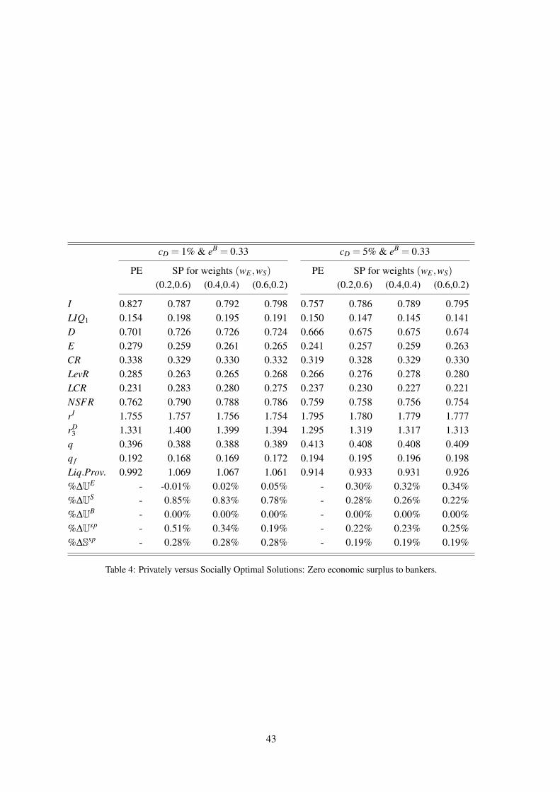
cD = 1% & eB = 0.33 cD = 5% & eB = 0.33
PE SP for weights (wE ,wS) PE SP for weights (wE ,wS)
(0.2,0.6) (0.4,0.4) (0.6,0.2) (0.2,0.6) (0.4,0.4) (0.6,0.2)
I 0.827 0.787 0.792 0.798 0.757 0.786 0.789 0.795LIQ1 0.154 0.198 0.195 0.191 0.150 0.147 0.145 0.141D 0.701 0.726 0.726 0.724 0.666 0.675 0.675 0.674E 0.279 0.259 0.261 0.265 0.241 0.257 0.259 0.263CR 0.338 0.329 0.330 0.332 0.319 0.328 0.329 0.330LevR 0.285 0.263 0.265 0.268 0.266 0.276 0.278 0.280LCR 0.231 0.283 0.280 0.275 0.237 0.230 0.227 0.221NSFR 0.762 0.790 0.788 0.786 0.759 0.758 0.756 0.754rI 1.755 1.757 1.756 1.754 1.795 1.780 1.779 1.777rD
3 1.331 1.400 1.399 1.394 1.295 1.319 1.317 1.313q 0.396 0.388 0.388 0.389 0.413 0.408 0.408 0.409q f 0.192 0.168 0.169 0.172 0.194 0.195 0.196 0.198Liq.Prov. 0.992 1.069 1.067 1.061 0.914 0.933 0.931 0.926%∆UE - -0.01% 0.02% 0.05% - 0.30% 0.32% 0.34%%∆US - 0.85% 0.83% 0.78% - 0.28% 0.26% 0.22%%∆UB - 0.00% 0.00% 0.00% - 0.00% 0.00% 0.00%%∆Usp - 0.51% 0.34% 0.19% - 0.22% 0.23% 0.25%%∆Ssp - 0.28% 0.28% 0.28% - 0.19% 0.19% 0.19%
Table 4: Privately versus Socially Optimal Solutions: Zero economic surplus to bankers.
43

Optimal Bank RegulationIn the Presence of Credit and Run Risk
Anil K Kashyap Dimitrios P. Tsomocos Alexandros P. Vardoulakis
Online Appendix
Appendix A reports derivations and results that were omitted in the main body of the paper.
Subsection A.1 provides additional details about the computation of the run threshold in the incom-
plete information game described in section 2.4. Section A.2 reports the detailed expressions for
the intermediation margins in section 3.2. Section A.3 derives the problem of the tools-augmented
Ramsey planner described in section 4.5. Section A.4 derives the equilibrium conditions when the
bank funds lending with her own funds. Section A.5 presents the problem when savers lend directly
to entrepreneurs. Section A.6 reports the planning outcomes when the planner can use other tools
to distort the deposit supply and loan demand schedules. Section A.7 presents the privately and
socially optimal solutions when interest rates are allowed to take negative values.
Appendix B presents an extension of the model where savers can also purchase equity in the bank
and the probability of bankruptcy in the final period conditional of the bank surviving the run is
endogenous.
A Additional derivations and computations
A.1 Run threshold
This section provides details about the calculation of the run threshold in equation (32). The util-
ity differential between waiting and withdrawing depends on the expected repayment on deposits,
which in turn is a function of the expected repayment on bank loans. Moreover, they both vary as
the portion of depositors, λ, varies from δ to θ∗. The entrepreneur always delivers in the good state
of the world and the bank is solvent when the portion of depositors withdrawing is δ. However, for
given ξ = ξ∗, bank profits fall as λ increases and there is a λ∈ (δ,θ∗) such that the bank is insolvent,
i.e., V D3g(ξ
∗,λ)< 1, for λ > λ. The threshold λ is calculated as the solution to equation(1− y(ξ∗, λ)
)· I ·(1+ rI)+LIQ2(ξ
∗, λ)−(
1− λ
)·D ·
(1+ rD
3)= 0. (A.1)
The bank is always insolvent in the bad state of the world, but the entrepreneur may not be.
The reason is that the entrepreneur’s loan obligation decreases as λ increases and the bank recalls
The views expressed in this paper are those of the authors and do not necessarily represent those of Federal ReserveBoard of Governors, anyone in the Federal Reserve System, the Bank of England Financial Policy Committee, or any ofthe institutions with which we are affiliated.
1
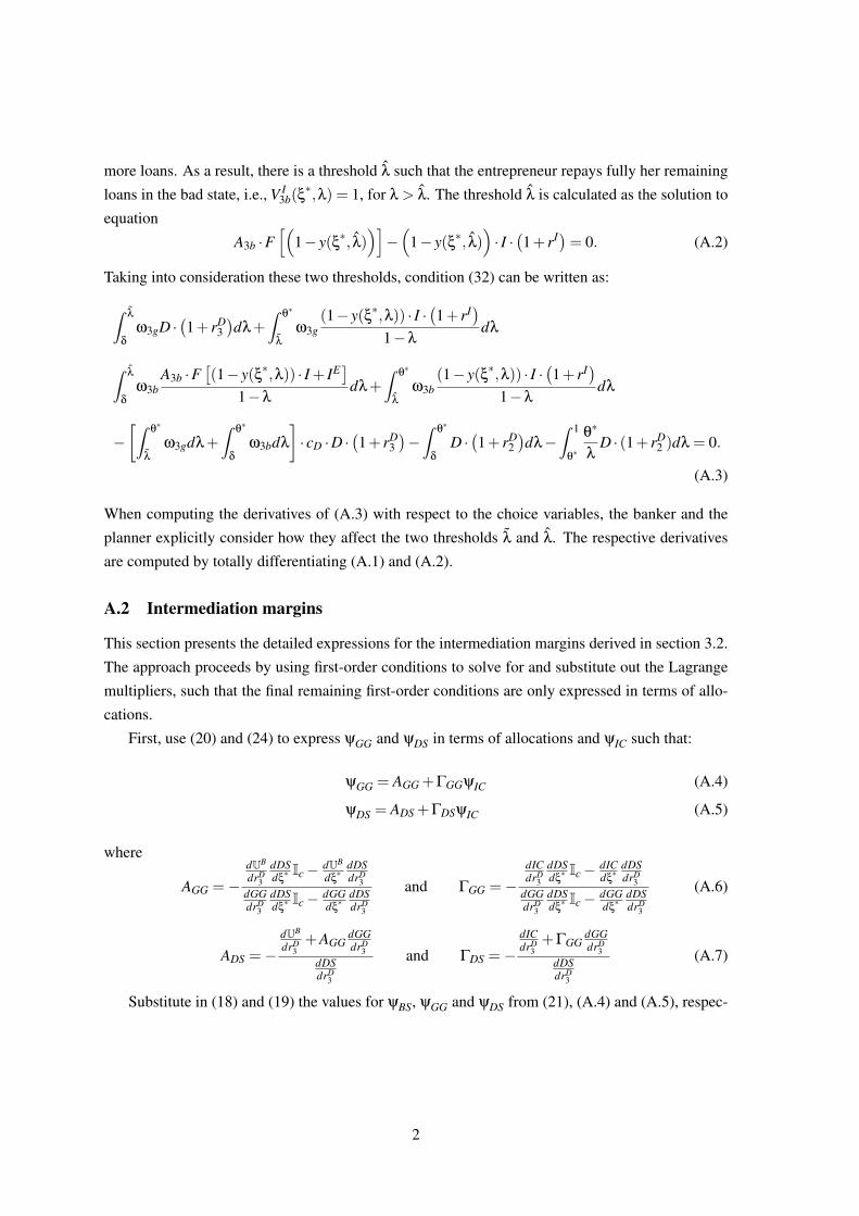
more loans. As a result, there is a threshold λ such that the entrepreneur repays fully her remaining
loans in the bad state, i.e., V I3b(ξ
∗,λ) = 1, for λ > λ. The threshold λ is calculated as the solution to
equation
A3b ·F[(
1− y(ξ∗, λ))]−(
1− y(ξ∗, λ))· I ·(1+ rI)= 0. (A.2)
Taking into consideration these two thresholds, condition (32) can be written as:
∫λ
δ
ω3gD ·(1+ rD
3)dλ+
∫θ∗
λ
ω3g(1− y(ξ∗,λ)) · I ·
(1+ rI
)1−λ
dλ
∫λ
δ
ω3bA3b ·F
[(1− y(ξ∗,λ)) · I + IE
]1−λ
dλ+∫
θ∗
λ
ω3b(1− y(ξ∗,λ)) · I ·
(1+ rI
)1−λ
dλ
−[∫
θ∗
λ
ω3gdλ+∫
θ∗
δ
ω3bdλ
]· cD ·D ·
(1+ rD
3)−
∫θ∗
δ
D ·(1+ rD
2)dλ−
∫ 1
θ∗
θ∗
λD · (1+ rD
2 )dλ = 0.
(A.3)
When computing the derivatives of (A.3) with respect to the choice variables, the banker and the
planner explicitly consider how they affect the two thresholds λ and λ. The respective derivatives
are computed by totally differentiating (A.1) and (A.2).
A.2 Intermediation margins
This section presents the detailed expressions for the intermediation margins derived in section 3.2.
The approach proceeds by using first-order conditions to solve for and substitute out the Lagrange
multipliers, such that the final remaining first-order conditions are only expressed in terms of allo-
cations.
First, use (20) and (24) to express ψGG and ψDS in terms of allocations and ψIC such that:
ψGG = AGG +ΓGGψIC (A.4)
ψDS = ADS +ΓDSψIC (A.5)
where
AGG =−dUB
drD3
dDSdξ∗ Ic− dUB
dξ∗
dDSdrD
3dGGdrD
3
dDSdξ∗ Ic− dGG
dξ∗
dDSdrD
3
and ΓGG =−dICdrD
3
dDSdξ∗ Ic− dIC
dξ∗
dDSdrD
3dGGdrD
3
dDSdξ∗ Ic− dGG
dξ∗
dDSdrD
3
(A.6)
ADS =−dUB
drD3+AGG
dGGdrD
3dDSdrD
3
and ΓDS =−dICdrD
3+ΓGG
dGGdrD
3dDSdrD
3
(A.7)
Substitute in (18) and (19) the values for ψBS, ψGG and ψDS from (21), (A.4) and (A.5), respec-
2
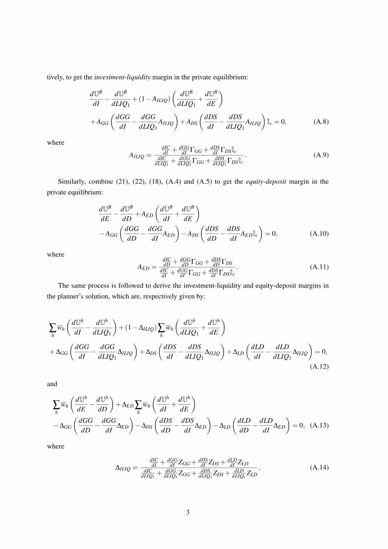
tively, to get the investment-liquidity margin in the private equilibrium:
dUB
dI− dUB
dLIQ1+(1−AILIQ)
(dUB
dLIQ1+
dUB
dE
)+AGG
(dGG
dI− dGG
dLIQ1AILIQ
)+ADS
(dDSdI− dDS
dLIQ1AILIQ
)Ic = 0, (A.8)
where
AILIQ =dICdI + dGG
dI ΓGG + dDSdI ΓDSIc
dICdLIQ1
+ dGGdLIQ1
ΓGG + dDSdLIQ1
ΓDSIc. (A.9)
Similarly, combine (21), (22), (18), (A.4) and (A.5) to get the equity-deposit margin in the
private equilibrium:
dUB
dE− dUB
dD+AED
(dUB
dI+
dUB
dE
)−AGG
(dGGdD− dGG
dIAED
)−ADS
(dDSdD− dDS
dIAEDIc
)= 0, (A.10)
where
AED =dICdD + dGG
dD ΓGG + dDSdD ΓDS
dICdI + dGG
dI ΓGG + dDSdI ΓDSIc
. (A.11)
The same process is followed to derive the investment-liquidity and equity-deposit margins in
the planner’s solution, which are, respectively given by:
∑h
wh
(dUh
dI− dUh
dLIQ1
)+(1−∆ILIQ)∑
hwh
(dUh
dLIQ1+
dUh
dE
)
+∆GG
(dGG
dI− dGG
dLIQ1∆ILIQ
)+∆DS
(dDSdI− dDS
dLIQ1∆ILIQ
)+∆LD
(dLDdI− dLD
dLIQ1∆ILIQ
)= 0,
(A.12)
and
∑h
wh
(dUh
dE− dUh
dD
)+∆ED ∑
hwh
(dUh
dI+
dUh
dE
)−∆GG
(dGGdD− dGG
dI∆ED
)−∆DS
(dDSdD− dDS
dI∆ED
)−∆LD
(dLDdD− dLD
dI∆ED
)= 0, (A.13)
where
∆ILIQ =dICdI + dGG
dI ZGG + dDSdI ZDS +
dLDdI ZLD
dICdLIQ1
+ dGGdLIQ1
ZGG + dDSdLIQ1
ZDS +dLD
dLIQ1ZLD
, (A.14)
3

∆ED =dICdD + dGG
dD ZGG + dDSdD ZDS +
dLDdD ZLD
dICdI + dGG
dI ZGG + dDSdI ZDS +
dLDdI ZLD
, (A.15)
∆GG =−∑h wh
[dUh
drD3
dDSdξ∗ − dUh
dξ∗
dDSdrD
3+(dLD
drI
)−1 dUh
drIdLDdξ∗
dDSdrD
3
]dGGdrD
3
dDSdξ∗ − dGG
dξ∗
dDSdrD
3+(dLD
drI
)−1 dLDdξ∗
dGGdrI
dDSdrD
3
, (A.16)
ZGG =−dICdrD
3
dDSdξ∗ − dIC
dξ∗
dDSdrD
3+(dLD
drI
)−1 dLDdξ∗
dICdrI
DSdrD
3
dGGdrD
3
dDSdξ∗ − dGG
dξ∗
dDSdrD
3+(dLD
drI
)−1 dLDdξ∗
dGGdrI
dDSdrD
3
, (A.17)
∆DS =−∑h wh
dUh
drD3+∆GG
dGGdrD
3dDSdrD
3
and ZDS =−dICdrD
3+ZGG
dGGdrD
3dDSdrD
3
, (A.18)
∆LD =−∑h wh
dUh
drI +∆GGdGGdrI
dLDdrI
and ZLD =−dICdrI +ZGG
dGGdrI
dLDdrI
. (A.19)
As discussed in the paper, the private intermediation margins differ from the planner’s in a
number of ways. Most importantly, the banker does not care how her choices directly affect the
utility of savers and entrepreneurs. Thus, additional terms enter into the planner’s solution, which
capture the direct total effect of the banking choices governing credit and run risk on savers’ and
entrepereneurs’ welfare. For example, the derivatives dU j/dξ∗, j = S,E, are present in (A.12) and
(A.13), but not in (A.8) and (A.10). These derivatives introduce a wedge between the private and
social intermediation margins. Additionally, the banker is protected by limited liability and will not
internalize all effects when contracts are incomplete, i.e., Ic = 0 in (A.12) and (A.13) contrary to
the planner’s intermediation margins where the relevant terms are always present.
A.3 Tools-augmented planner
In this section we specify the problem of the tools-augmented planner and show that (47) is (gener-
ically) a necessary and sufficient condition such that the social planner’s solution described in sec-
tion 3.1 can be decentralized as a private equilibrium by using regulatory tools T ∈ T. The tools-
augmented planner not only chooses optimally allocations and prices X ∈ X, but also the level of
tools T ∈ T and the multipliers ψT , which are the shadow values that the bank assigns to constraints
RC(T,X)≥ 0 in the new equilibrium. Her problem is:
maxX,T,ψT
Usp
s.t. B(X) = 0, RC(T,X)≥ 0, ILIQT(T,X ,ΨT ) = 0, IDT(T,X ,ΨT ) = 0, (A.20)
4

where ILIQT and IDT are the regulation-distorted margins given by (45) and (46).
The first-order condition with respect to X (similar to first-order condition (35)) are:
∑h={E,R,B}
whdUh
dX+ζBS
dBSdX
+ζICdICdX
+ζGGdGGdX
+ζLDdLDdX
+ζDSdDSdX
+∑T
ζTdRCdX
+ζILIQdILIQT
dX+ζID
dIDTdX
= 0, (A.21)
where ζT , ζILIQ and ζID are the multipliers the tool-augmented planner assigns to regulatory con-
straints RC(T,X) and the three regulation-distorted intermediation margins.
The first-order conditions with respect to the level of tools T are:
ζTdRCdT
+ζILIQdILIQT
dT+ζID
dIDTdT
= 0, (A.22)
and choosing optimally the multipliers ψT yields:
ζILIQdILIQT
dψT+ζID
dIDTdψT
= 0. (A.23)
To prove sufficiency, (47) implies that there need to be two regulatory tools such that a solution
to multipliers ψT can be obtained. In turn, this means that there are two first-order conditions of the
form in (A.22) and two of the form in (A.23). Conditions (A.23) can be written in matrix form as
transpose(∆RC) · transpose([ζILIQ ζID]) = 0. Given that ∆RC is invertible, ζILIQ = ζID = 0. Thus,
the only solution is one where all ζT , ζILIQ and ζED are zero and the first-order conditions (A.21)
coincide with the first-order conditions (35) of the social planner.
To prove necessity, suppose that (47) does not hold or in other words the span of ∆RC is less than
two. Using conditions (A.21) we can derive intermediation margins ILIQtap = ILIQsp + ILIQwedgetap
and IDtap = IDsp + IDwedgetap for the tool-augmented planner, where the wedges are linear combi-
nation of one multiplier ζT , ζILIQ and ζID. The social planner’s and tools-augmented planner’s
solutions coincide if both wedges are zero, which in principle is possible because there are three
multipliers, hence three degrees of freedom. However, equations (A.22) and (A.23) remove two
degrees of freedom. Hence, it is not possible to replicate the social planner’s solution with fewer
that two independent tools, which leads to a contradiction.
A.4 Equilibrium without deposit intermediation
The participation constraint (25) of the banker supposes that utility in autarky is the outside op-
tion. As already mentioned, we could consider the utility that the banker obtains by lending to
entrepreneurs using only her own funds as an outside option. This section derives the conditions
for the alternative outside option and shows that for the equilibrium considered in section 3.3 the
autarkic utility is the relevant outside option.
5
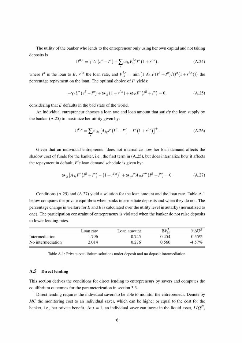
The utility of the banker who lends to the entrepreneur only using her own capital and not taking
deposits is
UB,n = γ ·U(eB− In)+∑
sω3sV
I,n3s In (1+ rI,n), (A.24)
where In is the loan to E, rI,n the loan rate, and V I,n3s = min
(1,A3sF(IE + In)/(In(1+ rI,n))
)the
percentage repayment on the loan. The optimal choice of In yields:
−γ ·U ′(eB− In)+ω3g
(1+ rI,n)+ω3bF ′
(IE + In)= 0, (A.25)
considering that E defaults in the bad state of the world.
An individual entrepreneur chooses a loan rate and loan amount that satisfy the loan supply by
the banker (A.25) to maximize her utility given by:
UE,n = ∑s
ω3s[A3gF
(IE + In)− In (1+ rI,n)]+ . (A.26)
Given that an individual entrepreneur does not internalize how her loan demand affects the
shadow cost of funds for the banker, i.e., the first term in (A.25), but does internalize how it affects
the repayment in default, E ′s loan demand schedule is given by:
ω3g[A3gF ′
(IE + In)− (1+ rI,n)]+ω3bInA3bF ′′
(IE + In)= 0. (A.27)
Conditions (A.25) and (A.27) yield a solution for the loan amount and the loan rate. Table A.1
below compares the private equilibria when banks intermediate deposits and when they do not. The
percentage change in welfare for E and B is calculated over the utility level in autarky (normalized to
one). The participation constraint of entrepreneurs is violated when the banker do not raise deposits
to lower lending rates.
Loan rate Loan amount EV I3b %∆UE
Intermediation 1.796 0.745 0.454 0.55%No intermediation 2.014 0.276 0.560 -4.57%
Table A.1: Private equilibrium solutions under deposit and no deposit intermediation.
A.5 Direct lending
This section derives the conditions for direct lending to entrepreneurs by savers and computes the
equilibrium outcomes for the parameterization in section 3.3.
Direct lending requires the individual savers to be able to monitor the entrepreneur. Denote by
MC the monitoring cost to an individual saver, which can be higher or equal to the cost for the
banker, i.e., her private benefit. At t = 1, an individual saver can invest in the liquid asset, LIQdl ,
6

or lend to the entrepreneur, Idl , at interest rate rI,dl . In the intermediate period, she would liquidate
all her loans if she turns out to be impatient. Otherwise, the saver waits until the final period and
receives the percentage repayment on the loans she made. Her utility under direct lending is given
by:
US,dl =U1
(cdl
1
)+δ
∫ξ
ξ
U2
(cdl
2 ; i) dξ
∆ξ
+(1−δ)∑s
ω3sU3
(cdl
3 ; p),
where cdl1 = eS
1− Idl − LIQdl , cdl2 = eS
2 + LIQdl + ξ · Idl , and cdl3 = eS
2 + LIQdl +(V I,dl3s − cD · Idl) ·
Idl · (1+ rI,dl)−MC. Moreover, V I,dl3s = min[1,A3s ·F(IE + Idl)/(Idl · (1+ rI,dl))] is the percentage
repayment on the loan and Idl is the indicator function for default.
Under the assumption that an individual saver lends to an individual entrepreneur, the former
will internalize how her loan extension affects the expected delivery in default (much like the banker
does). Hence, the optimal choice of lending, Idl , yields:
−U ′1(
cdl1
)+δ
∫ξ
ξ
ξ ·U ′2(
cdl2 ; i) dξ
∆ξ
+β2(1−δ) ·
[ω3g
(1+ rdl
)+ω3b
(A3bF ′
(IE + Idl
)− cD
)]= 0
(A.28)
where we have used the facts that U ′3(·; p) = β2 and that the entrepreneur would default, in equilib-
rium, in the bad state.
Similarly, the optimal choice of liquid holdings, LIQdl , yields:
−U ′1(
cdl1
)+δ
∫ξ
ξ
U ′2(
cdl2 ; i) dξ
∆ξ
+β2(1−δ)+νLIQDL = 0, (A.29)
where νLIQDL is the Lagrange multiplier on the constraint LIQDL ≥ 0.
The utility of an individual entrepreneur
UE,dl = δ ·UE,aut +(1−δ) ·ω3g
[A3gF
(eE + Idl
)− Idl ·
(1+ rdl
)], (A.30)
given that E invests all of her wealth in the project, i.e., IE = eE . With probability δ an individual
entrepreneur has her project liquidated and continues to produce only with her own capital. As a
result, she enjoys the same utility as in autarky. With probability 1−δ, the saver does not liquidate
the project and the entrepreneur defaults in that bad state. The entrepreneur chooses the loan amount,
Idl , and the loan rate, rdl , that satisfy (A.28) to maximize (A.30). Consistent with our analysis in
the rest of the paper, the entrepreneur internalizes her effect on the marginal payoff accruing to the
saver, but takes the other forces determining saver’s costs of funds (marginal utilities at t = 1 and
t = 2) as given. Thus, the optimal loan demand by the entrepreneur is:
ω3g
[A3gF ′
(eE + Idl
)−(
1+ rdl)]
+ω3bA3bF ′′(
eE + Idl)
Idl = 0. (A.31)
7

Conditions (A.28), (A.29) and (A.31) jointly determine Idl , LIQdl and rdl in equilibrium. Using
the parameterization in section 3.3 and setting MC equal to PB, the utility of savers is 0.07% higher
under bank intermediation compared to direct lending which, in turn, is higher than the utility in
autarky. By increasing MC we can obtain equilbria where direct lending delivers lower utility to
savers and eventually is dominated by autarky. In addition, the utility of entrepreneurs is higher
than in autarky, thus they are willing to borrow directly from savers.
A.6 Additional distortionary tools
This section extends the analysis in section 3.3 by allowing the planner to use tools to distort the
deposit supply and loan demand schedules of savers and entrepreneurs. We consider generic tools,
τDS for the deposit supply schedule, and τLD for the loan demand schedule, and discuss how they
can be implemented in practice.
The deposit supply schedule (7) that the planner faces becomes:
−U ′1 (c1)+(1+ rD
2)[
∑t=2,3
{∫ξ∗
ξ
θ(ξ,1) ·E jU ′t (cts ( j,1) ; j)dξ
∆ξ
}+δ
∫ξ
ξ∗
U ′2 (c2 (i,1) ; i)dξ
∆ξ
]
+(1−δ)∫
ξ
ξ∗ ∑
sω3sU ′3 (c3s (p,0) ; p) ·
(V D
3s (ξ,δ)− cD · Id)· (1+ rD
3 )dξ
∆ξ
+νD + τDS = 0. (A.32)
To the extent that savers supply deposits, i.e., νD = 0, the planner can distort their willingness to
hold deposits at given deposit rates by varying the level of the distortionary tool τDS. In other words,
the planner can set τDS 6= 0, which implies that (A.32) stops being a constraint in her optimization
problem (33) and ζDS = 0 in (35). The intervention can be implemented, for example, either as a
tax on the supply of deposits at t = 1 or as a tax on the interest income accruing to late depositors
at t = 3 when the bank is solvent. In the first case, the tax can be computed as −τDS/U ′1(c1), while
in the second as −τDS/(ω3g(1−q) · (1−δ) ·U ′3 (c3g (p,0) ; p) · (1+ rD
3 )). If τDS < 0, then a tax is
levied, while τDS > 0 implies a subsidy. We assume that the planner rebates the tax proceeds back to
the same agents in the same period in a lump-sum fashion in order to neutralize any income effects.
Similarly, the loan demand schedule (27) becomes:
∫ξ
ξ∗(1− y(ξ,δ))
[A3gF ′
(IE +(1− y(ξ,δ)) · I
)− (1+ rI)+ I · ∂LS
∂I
(∂LS∂rI
)−1]
dξ
∆ξ
+ τLD = 0.
(A.33)
The planner can distort the willingness of entrepreneurs to borrow by varying the level of the
distortionary tool τLD. such that if τLD 6= 0, then ζLD = 0 in (35). The intervention can be imple-
mented with a tax on loan repayment in the good state of the world, which can be computed as
−τLD/
(∫ξ
ξ∗ (1− y(ξ,δ))(1+ rI)dξ/∆ξ
). If τLS < 0, then a tax is levied, while τLS > 0 implies a
8

subsidy. A tax can also be implemented with restrictions on the maximum loan-to-value ratio for
entrepreneurial loans, i.e., I ≤ LTV/(1−LTV ) · IE where LTV is the loan-to-value limit. Then, τLD
is the value of the Lagrange multiplier on the LTV constraint. Note that this limit is imposed on the
entrepreneur rather than the banker, because the objective is to distort the loan demand schedule.
Table A.2 below reports the planning equilibria under two sets of weights when distortionary
tools are available (using the parameterization discussed in section 3.3). Comparing the planning
outcomes with and without distortionary tools, we can observe that the planner can improve so-
cial gains if she is endowed with more tools. The reason is that both savers and entrepreneurs do
not internalize how their behavior affects the aggregate bank variables, and most importantly the
probability of a run.
Nevertheless, there are three important observations about this extension of the model. First,
banking regulation is still needed to implement socially optimal outcomes. The additional dis-
tortionary tools affect the deposit supply and loan demand schedules, but do not correct for the
distortions in the banker’s optimization condition. Capital and liquidity regulation are required for
the latter. Second, the use of the distortionary tools has implications for the allocation of social
gains. While the banker remains at her participation constraint, either the saver or the entrepreneur
can be made better-off when these tools are used compared to the social planning outcomes without
them. Third, a tax that restricts the supply of deposits can be beneficial for savers. In particular,
the bank has to offer higher deposit rates to attact deposits and the smaller reliance on deposits in
combination with capital and liquidity regulations improves the bank’s stability. Liquidity provi-
sion is lower, but this does not hurt savers overall because they are able to self-insure by holding
the liquid asset. The benefits are smaller when savers are not allowed to self-insure. Moreover,
entrepreneurs are worse-off because the level of funds channeled through the bank goes down and
they are driven to their participation constraint. As a result, τLD cannot be combined in this example
with τLD because there are no additional social gains to be made.
A.7 Negative interest rates
This section relaxes the assumption about the non-negativity of the early deposit rate, rD2 , and shows
that our conclusions about the necessity for capital and liquidity regulations carry over. Table A.3
reports the private and socially optimal outcomes for negative rD2 .
Negative early deposit rates reduce the probability of a run, since both the savers’ incentive
to run and the bank’s liquidity needs are lower. The banker will weigh the reduction in the run
probability to the potential increase in late deposit rates when choosing to set early deposit rates
negative. However, the banker is not able to decrease rD2 all the way to the level that the probability
of a run is zero, because she would either need to offer very high rD3 , which eliminates her own
profits, or violate the participation constraint of savers. In the private equilibrium in Table A.3
savers are driven to their participation contraint (9). So merely allowing for negative rates does not
allow the private sector to deliver run-free banking.
The planner can reduce the early deposit rate all the way to the point that runs are ruled out.
9
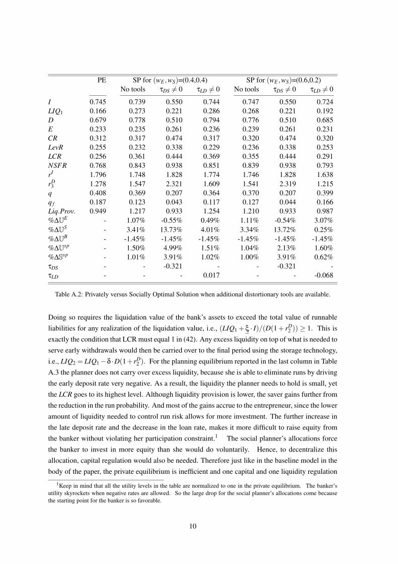
PE SP for (wE ,wS)=(0.4,0.4) SP for (wE ,wS)=(0.6,0.2)No tools τDS 6= 0 τLD 6= 0 No tools τDS 6= 0 τLD 6= 0
I 0.745 0.739 0.550 0.744 0.747 0.550 0.724LIQ1 0.166 0.273 0.221 0.286 0.268 0.221 0.192D 0.679 0.778 0.510 0.794 0.776 0.510 0.685E 0.233 0.235 0.261 0.236 0.239 0.261 0.231CR 0.312 0.317 0.474 0.317 0.320 0.474 0.320LevR 0.255 0.232 0.338 0.229 0.236 0.338 0.253LCR 0.256 0.361 0.444 0.369 0.355 0.444 0.291NSFR 0.768 0.843 0.938 0.851 0.839 0.938 0.793rI 1.796 1.748 1.828 1.774 1.746 1.828 1.638rD
3 1.278 1.547 2.321 1.609 1.541 2.319 1.215q 0.408 0.369 0.207 0.364 0.370 0.207 0.399q f 0.187 0.123 0.043 0.117 0.127 0.044 0.166Liq.Prov. 0.949 1.217 0.933 1.254 1.210 0.933 0.987%∆UE - 1.07% -0.55% 0.49% 1.11% -0.54% 3.07%%∆US - 3.41% 13.73% 4.01% 3.34% 13.72% 0.25%%∆UB - -1.45% -1.45% -1.45% -1.45% -1.45% -1.45%%∆Usp - 1.50% 4.99% 1.51% 1.04% 2.13% 1.60%%∆Ssp - 1.01% 3.91% 1.02% 1.00% 3.91% 0.62%τDS - - -0.321 - - -0.321 -τLD - - - 0.017 - - -0.068
Table A.2: Privately versus Socially Optimal Solution when additional distortionary tools are available.
Doing so requires the liquidation value of the bank’s assets to exceed the total value of runnable
liabilities for any realization of the liquidation value, i.e., (LIQ1 + ξ · I)/(D(1+ rD2 )) ≥ 1. This is
exactly the condition that LCR must equal 1 in (42). Any excess liquidity on top of what is needed to
serve early withdrawals would then be carried over to the final period using the storage technology,
i.e., LIQ2 = LIQ1−δ ·D(1+ rD2 ). For the planning equilibrium reported in the last column in Table
A.3 the planner does not carry over excess liquidity, because she is able to eliminate runs by driving
the early deposit rate very negative. As a result, the liquidity the planner needs to hold is small, yet
the LCR goes to its highest level. Although liquidity provision is lower, the saver gains further from
the reduction in the run probability. And most of the gains accrue to the entrepreneur, since the lower
amount of liquidity needed to control run risk allows for more investment. The further increase in
the late deposit rate and the decrease in the loan rate, makes it more difficult to raise equity from
the banker without violating her participation constraint.1 The social planner’s allocations force
the banker to invest in more equity than she would do voluntarily. Hence, to decentralize this
allocation, capital regulation would also be needed. Therefore just like in the baseline model in the
body of the paper, the private equilibrium is inefficient and one capital and one liquidity regulation
1Keep in mind that all the utility levels in the table are normalized to one in the private equilibrium. The banker’sutility skyrockets when negative rates are allowed. So the large drop for the social planner’s allocations come becausethe starting point for the banker is so favorable.
10

is required to match the social planner’s allocations.
PE SP
I 0.870 1.492LIQ1 0.123 0.015D 0.742 1.343E 0.251 0.164CR 0.288 0.110LevR 0.253 0.109LCR 0.282 1.000NSFR 0.715 0.560rI 1.675 1.313rD
2 -0.370 -0.976rD
3 1.030 3.644q 0.193 0.000q f 0.099 0.000Liq.Prov. 0.946 0.724%∆UE - 23.74%%∆US - 29.14%%∆UB - -27.01%%∆Usp - 15.75%%∆Ssp - 8.63%
Table A.3: Privately versus Socially Optimal Solutions for rD2 < 0. The planning outcomes are for weights
(wE ,wS) = (0.4,0.4). We have added a fixed number (equal to 1) to the utility of impatient depositors,because it takes negative values for q = 0 as early consumption, c2(i), is less than 1. This does not affectmarginal decisions and equilibrium outcomes, but it allows the easy comparison of the Liq.Prov. ratio acrossequilibria, which would otherwise have a negative value for q = 0.
11

B Extended model
This section extends the baseline model so that savers can also purchase equity in the bank and the
probability of bankruptcy in the final period conditional on the bank surviving the run is endoge-
nous.
The first modification implies that the banker and the planner have an alternative source of
funding apart from the equity contributed by the banker and deposits offered by savers. We will
refer to equity contributed by bankers and savers as “inside” and “outside” equity, respectively.
The introduction of an additional source of funding adds another intermediation margin for banking
decisions. We show that this margin is also distorted and that a planner would need an additional
tool on top of a capital and a liquidity regulation to fully implement a solution with positive outside
equity.
The second modification allows us to examine how regulation differentially affects run risk and
credit risk. To do so, we introduce a third "medium" state for the realization of the productivity
shock in the final period, which is between the level in the good and the bad state. Thus, the state
space at t = 3 is s ∈ {g,m,b} and the productivity realization satisfy A3g > A3m > A3b. We focus on
cases in which entrepreneurs default in states m and b, while they fully repay in state g. The bank
is solvent is state g and defaults in state b, while the bankruptcy decision depends on the realization
of ξ in state m. Hence, there is a threshold ξ ∈(
ξ∗,ξ)
such that the bank is solvent in state m
only if the realization of the liquidation value is higher than ξ. The threshold is endogenous and
depends on the balance sheet of the bank. Thus, it plays a critical role in the expected probability
of bank default and the benefit of raising equity to reduce expected bankruptcy costs.2 We also
consider a general specification for bankruptcy costs and introduce investment adjustment costs for
entrepreneurs when their loans are recalled and investment liquidated.
These modifications allow us to study equilibria where the planner chooses positive outside
equity and there is room for redistributive effects of regulation. To avoid repeating ourselves, we
only present the equations where these modifications enter.
B.1 Modified savers’ problem
As in the baseline model, savers invest in bank deposits and the liquid asset at t = 1 to maximize
their lifetime expected utility (6). But, they can additionally buy bank (outside) equity shares, ES,
in a primary market at a price P per share. Equity is valuable because of the dividends paid on each
share, DPS3s(ξ,λ), at t = 3. Recall that in the baseline model we did not distinguish between bank
profits and dividends per share given that the banker is the sole equity-holder. We will be precise
2Having only three levels of productivity does not change the fundamental economic outcomes in the extended model.In particular, even with many more outcomes for technology there are fundamentally only three different types of out-comes. For some realizations of productivity the resources are sufficient so that the loans are fully paid and in this casethe deposits are also fully paid. Conversely, it is possible that the investment outcome is so poor that the loan repay-ment is so low that the depositors can never be fully paid. Finally, there are interim cases where the loans may not becompletely paid, but the bank still can fully pay deposits. Nothing in the analysis would change if we had many morestates.
12

about how the dividends per share are determined in the modified banker’s problem below. As a
result, the budget constraint at t = 1 –equation (1)– becomes:
c1 = eS1−D−P ·ES−LIQS
1. (B.1)
Each share can be re-traded in a secondary market as a price Psec(ξ,λ). In a run, equity is
worthless, i.e., Psec(ξ,1) = 0 and DPS3s(ξ,1) = 0 because the bank is liquidated. Patient savers will
enter the secondary market to buy equity from impatient savers. The patient savers’ total funds are
the sum of their new endowment, eS2, and their liquid holdings carried over from the first period,
LIQS1. The patient savers total equity holdings after trading are ES
sec(ξ,λ). Thus, the net purchase
is Psec(ξ,δ) · (ESsec(ξ,λ)−ES) and the remaining resources are transferred to t = 3 using the storage
technology. Conditional on a run ocurring, the consumption of a saver of type j is still given by (2).
However, the consumption of an impatient saver when a run does not occur –equation (3)– is now
given by:
c2(i,Iw = 1) = D(1+ rD
2)+LIQS
1 +Psec(ξ,λ)+ eS2. (B.2)
Similarly, the consumption at t = 3 of a patient saver who chooses to wait or withdraw –
equations (4) and (5) respectively– will be given by3
c3s (p,Iw = 0) = ESsec (ξ,λ,Iw = 0)DPS3s (ξ,λ)+Psec (ξ,λ)
(ES−ES
sec (ξ,λ,Iw = 0))
+(V D
3s (ξ,λ)− cD(D) · Id)
D(1+ rD
3)+LIQS
1 + eS2, (B.3)
or
c3s (p,Iw = 1) = ESsec (ξ,λ,Iw = 1)DPS3s (ξ,λ)+Psec (ξ,λ)
(ES−ES
sec (ξ,λ,Iw = 1))
+D(1+ rD
2)+LIQS
1 + eS2. (B.4)
Since the individual saver takes the bank dividends as given, the optimal decision to purchase
equity, ES, in the primary market is chosen so that
ES :−P ·U ′1 (c1)+
no run︷ ︸︸ ︷∑
t=2,3
{∫ξ
ξ∗E jU ′t (cts ( j,Iw) ; j) ·Psec (ξ,δ)
1∆ξ
dξ
}+νES = 0, (B.5)
3In the extended model we consider a more general function for the bankruptcy costs given by cD(D) = cD ·DφD ,φD ≥ 0. The more general specification can enhance the risk-sharing role of equity because different allocations implydifferent marginal bankruptcy costs. Savers’ take cD(D) as given since it is a function of the total deposits in the bank.Hence, the deposit supply equation (7) has the same functional form in the extended model with the difference that themarginal cost depends on D in equilibrium. The banker and the planner account for this dependance.
13

where ES stands for equity supply and νES is the multiplier on the no short-sale constraint ES ≥0. Condition (B.5) says that savers equate the marginal utility of lost consumption from buying
one bank share at price P to the expected marginal utility gain from the value of the share in the
future, Psec(ξ,δ). The share only has any value if the bank survives a run, since otherwise equity is
worthless.
The value of equity that emerges from the secondary market trading satisfies
Psec(ξ,δ) = ∑s
ω3sDPS3s(ξ,δ), (B.6)
i.e., the secondary equity price is equal to the expected value of future dividends because patient
savers have linear utility at t = 3 and their outside option pays zero interest. If a run does not occur,
impatient savers sell their bank shares to patient savers. Market clearing requires the equity holdings
of each individual patient saver at t = 3 be such that ESsec(ξ,δ) = ES/(1−δ).
Before turning to the modified problems of the banker and the entrepreneur, it is easy to show
that the global game analysis in section 2.4 remains intact (once we account for the additional state
m). The reason is that because of quasi-linear utilities the expected utility differential between wait-
ing and withdrawing conditional on the bank surviving the run –upper part in (31)– is not affected
by the decision to purchase outside equity. To be more precise, the expected utility differential is the
difference in expected consumption in (B.3) and expected consumption in (B.4), which differ in two
ways. One arises from the different equity holding after secondary trading for a saver that waits and
a saver that withdraws, and the other comes because the person who waits will receive a late deposit
payment, while the other person will get her deposits early and transfer them to period 3 using the
liquid asset. However, the demand for equity in the secondary market determines the secondary
equity price Psec(ξ,λ) =∑s
ω3sDPS3s(ξ,λ). Substituting the secondary price in (B.3) and (B.4), the
expected utility differential between waiting and withdrawing conditional on the bank surviving the
run is ∑s{ω3s(V D
3s(ξ,λ)− cD(D) · Id)D(1+ rD
3)}−D
(1+ rD
2).4
B.2 Modified banker’s problem
The banker makes the same decisions as in the baseline model, but additionally needs to decide
how much outside equity to raise from savers. The equity shares in the bank will be split between
the banker and savers and the respective holdings are denoted by EB and ES. At this point we
distinguish between the initial equity, EB0 , that the banker holds, and the additional equity, EB
1 , that
4The linearity of utility from consumption at t = 3 simplifies the run decision substantially since the expectedutility differential between waiting and withdrawing, given by equation (31), depends only on predetermined vari-ables and not on actions taken after the run decision, such as trading in the secondary equity market. The terms∑s
ω3sESsec(ξ,δ,Iw)(DPS3s(ξ,δ)−Psec(ξ,δ)), for both Iw = 0 and Iw = 1, in patient agents’ period 3 expected utility
drop out. This is an outcome of the linear preference at t = 3 and is true for any portion of savers λ deciding to withdraw.As a result, the computation of the run threshold in the global game is largely simplified, because the distribution ofequity holdings between patient savers that choose to withdraw and those that choose to wait does not matter for theutility differential.
14

she decides to put into the bank at price P by participating in the primary equity market at t = 1.
This distinction was inconsequential in the baseline model that the banker is the sole owner of the
bank. Hence, the total share holdings of the banker are EB = EB0 +EB
1 . Pinning down the share of
ownership is important because the profits accruing to the banker depend on her relative holdings,
EB/(EB +ES), or in other words she will receive a dividend per share for each of the EB she holds.
The banker’s utility –equation (10)– changes to:
UB = γ ·U(eB−P ·EB
1)+
no run︷ ︸︸ ︷EB
∫ξ
ξ∗ ∑
sω3sDPS3s(ξ,δ)
1∆ξ
dξ . (B.7)
The banker trades off foregoing current consumption to investing in equity and receiving dividends
in the future. Note that the banker gets to consume her share of dividends only if the bank survives
the run. The banker “buys" additional equity at the same price at which she issues equity to savers.
The balance sheet constraint at t = 1 –equation (11)– becomes:
BS : I+LIQ1 = D+CEQ, (B.8)
where CEQ = P ·(ES +EB
1)+EB
0 is the total common equity.
Raising outside equity does not affect the balance sheet constraints at t = 2, thus the probability
that a depositors is served, θ(ξ,λ), in a run are given by (12) and the fraction of loans recalled,
y(ξ,λ), when a run does not occur are given by (13). The dividends per share are the total dividends
divided by the total number of shares, i.e.,
DPS3s (ξ,λ) =DIV3s(ξ,λ)
EB +ES , (B.9)
where DIV3s(ξ,λ) are given by (14).
Moreover, the banker will choose to monitor if her share of the dividends rather than total
dividend are higher than the private benefit. Thus, the incentive compatibility constraint –equation
(17)– becomes:
IC : EB∑
sω3sDPS3s(ξ
∗,δ)−PB≥ 0. (B.10)
Finally, the second modification to the baseline model implies an endogenous bankruptcy thresh-
old, ξ, in state m is determined by the following equation:(1− y
(ξ,δ))
V I3m
(ξ,δ)
I(1+ rI)+LIQ2
(ξ,δ)− (1−δ)D
(1+ rD
3)= 0. (B.11)
We now turn into describing how the optimality conditions are altered and what are the new
optimality conditions with respect to outside equity and the equity price. We will focus attention to
incomplete funding contracts, i.e., deposit contracts specify the tuple (D,rD2 ,r
D3 ) and equity contracts
15

specify the tuple (EB1 ,E
S,P)The marginal effect of investment on banker’s utility in the optimality condition for loans, I
–equation (18)– becomes:
dUB
dI=
EB
EB +ES
no default, state g︷ ︸︸ ︷∫
ξ
ξ∗
{ω3g
(1+ rI)} 1
∆ξ
dξ+
no default, state m︷ ︸︸ ︷∫ξ
ξ
{ω3mA3mF ′
(IE +(1− y(ξ,δ)) I
)} 1∆ξ
dξ
. (B.12)
As shown in (B.12), limited liability means that the banker still only internalizes states where she is
solvent.Similarly, the marginal effect of investment on banker’s utility in the optimality condition for
first period liquid assets, LIQ1 –equation (19)– becomes:
dUB
dLIQ1=
EB
EB +ES
no default, state g︷ ︸︸ ︷∫
ξ
ξ∗
{ω3g
(1+ rI) 1
ξ
}1
∆ξ
dξ+
no default, state m︷ ︸︸ ︷∫ξ
ξ
{ω3mA3mF ′
(IE +(1− y(ξ,δ)) I
) 1ξ
}1
∆ξ
dξ
.(B.13)
The optimal choice of the run threshold –equation (20)– becomes
−EB∑
sω3sDPS3s(ξ
∗,δ)1
∆ξ
+ψICdICdξ∗ +ψGG
dGGdξ∗ = 0. (B.14)
The optimal choice of liquidity holdings, LIQ2(ξ,δ), at t = 2 after the run uncertainty is resolved
is given by:
EB
EB +ES
(ω3g
[1−
V I3g
(1+ rI
)ξ
]+ω3m
[1−
V I3m
(1+ rI
)ξ
]· (1− Id)
)+ν
LIQ2(ξ,δ)= 0, ∀ ξ≥ ξ∗,
(B.15)
where νLIQ2(ξ,δ) is the multiplier on the short-sale constraint LIQ2(ξ,δ)≥ 0.
Turning to the deposit contract, the marginal effects of the deposit contract terms on banker’sutility in the optimality conditions (22) to (24)–become:
dUB
dD=− EB
EB +ES
no default, state g︷ ︸︸ ︷∫
ξ
ξ∗
{ω3g
(1+ rI) δ
(1+ rD
2)
ξ+(1−δ)
(1+ rD
3)} 1
∆ξ
dξ
no default, state m︷ ︸︸ ︷+∫
ξ
ξ
{ω3mA3mF ′
(IE +(1− y(ξ,δ)) I
) δ(1+ rD
2)
ξ+(1−δ)
(1+ rD
3)} 1
∆ξ
dξ
, (B.16)
16
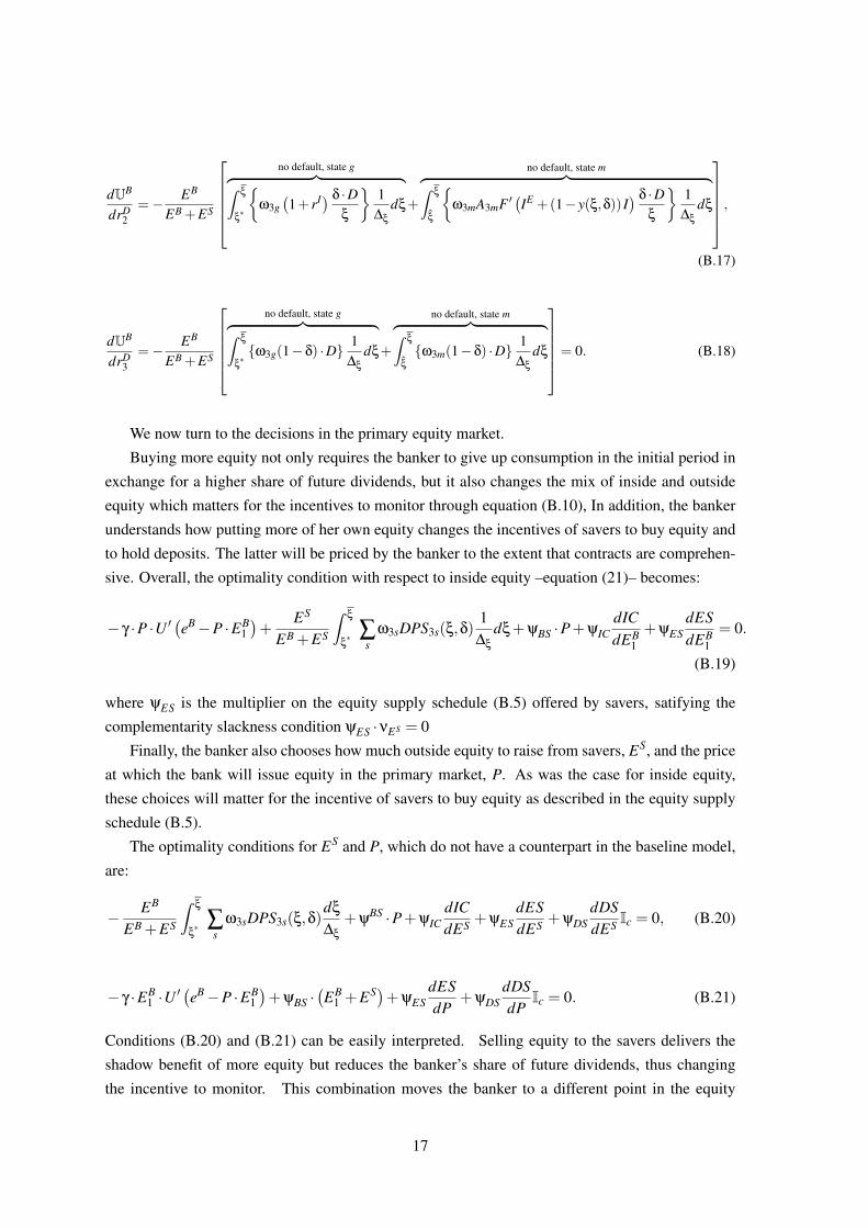
dUB
drD2
=− EB
EB +ES
no default, state g︷ ︸︸ ︷∫
ξ
ξ∗
{ω3g
(1+ rI) δ ·D
ξ
}1
∆ξ
dξ+
no default, state m︷ ︸︸ ︷∫ξ
ξ
{ω3mA3mF ′
(IE +(1− y(ξ,δ)) I
) δ ·Dξ
}1
∆ξ
dξ
,(B.17)
dUB
drD3
=− EB
EB +ES
no default, state g︷ ︸︸ ︷∫
ξ
ξ∗{ω3g(1−δ) ·D} 1
∆ξ
dξ+
no default, state m︷ ︸︸ ︷∫ξ
ξ
{ω3m(1−δ) ·D} 1∆ξ
dξ
= 0. (B.18)
We now turn to the decisions in the primary equity market.
Buying more equity not only requires the banker to give up consumption in the initial period in
exchange for a higher share of future dividends, but it also changes the mix of inside and outside
equity which matters for the incentives to monitor through equation (B.10), In addition, the banker
understands how putting more of her own equity changes the incentives of savers to buy equity and
to hold deposits. The latter will be priced by the banker to the extent that contracts are comprehen-
sive. Overall, the optimality condition with respect to inside equity –equation (21)– becomes:
− γ ·P ·U ′(eB−P ·EB
1)+
ES
EB +ES
∫ξ
ξ∗ ∑
sω3sDPS3s(ξ,δ)
1∆ξ
dξ+ψBS ·P+ψICdICdEB
1+ψES
dESdEB
1= 0.
(B.19)
where ψES is the multiplier on the equity supply schedule (B.5) offered by savers, satifying the
complementarity slackness condition ψES ·νES = 0
Finally, the banker also chooses how much outside equity to raise from savers, ES, and the price
at which the bank will issue equity in the primary market, P. As was the case for inside equity,
these choices will matter for the incentive of savers to buy equity as described in the equity supply
schedule (B.5).
The optimality conditions for ES and P, which do not have a counterpart in the baseline model,
are:
− EB
EB +ES
∫ξ
ξ∗ ∑
sω3sDPS3s(ξ,δ)
dξ
∆ξ
+ψBS ·P+ψIC
dICdES +ψES
dESdES +ψDS
dDSdES Ic = 0, (B.20)
− γ ·EB1 ·U ′
(eB−P ·EB
1)+ψBS ·
(EB
1 +ES)+ψESdESdP
+ψDSdDSdP
Ic = 0. (B.21)
Conditions (B.20) and (B.21) can be easily interpreted. Selling equity to the savers delivers the
shadow benefit of more equity but reduces the banker’s share of future dividends, thus changing
the incentive to monitor. This combination moves the banker to a different point in the equity
17

supply schedule of the savers. Finally, a higher equity issuance price affects the banker’s current
consumption negatively, because she has to pay this price, but has a positive balance sheet effect
and allows the banker to move at a different point on the savers’ equity supply schedule.
B.3 Modified entrepreneurs’ problem
As in the baseline model, the entrepreneur uses her own capital and borrows from the bank to invest
in the project. The loan contract specifies the loan amount and the loan rate. As already mentioned,
the entrepreneur repays her loan only if state g realizes. We, additionally, introduce adjustment
costs when part of entrepreneur’s initial investment is liquidated. These costs are paid by the en-
trepreneur in the intermediate period and are a function of the required adjustment, cI (y(ξ,δ) · I) =cI (y(ξ,δ) · I)φI , where cI > 0, φI ≥ 0. For simplicity, we assume that E pays these costs out of new
endowment, eE2 , she receives at t = 2. Note that E cannot invest in more long-term projects at t = 2,
thus she consumes at t = 3 what is left of the period 2 endowment after paying the adjustment costs.
Hence, the utility of an individual entrepreneur –equation (26)– becomes:
UE = ∑s
ω3s
no run︷ ︸︸ ︷∫
ξ
ξ∗
[A3sF
(IE +(1− y(ξ,δ))I
)− (1− y(ξ,δ))I(1+ rI)
]+ dξ
∆ξ
+
run︷ ︸︸ ︷∫ξ∗
ξ
A3sF(IE)dξ
∆ξ
+ eE
2 −∫
ξ
ξ
cI (y(ξ,δ) · I)dξ
∆ξ︸ ︷︷ ︸adjustment costs
. (B.22)
The optimal loan demand of an individual entrepreneur –equation (27)– becomes:
LD : ω3g
∫ξ
ξ∗(1− y(ξ,δ))
[A3gF ′
(IE +(1− y(ξ,δ)) · I
)− (1+ rI)+ I · ∂LS
∂I
(∂LS∂rI
)−1]
dξ
∆ξ
−∫
ξ
ξ
y(ξ,δ) · c′I (y(ξ,δ) · I)dξ
∆ξ
= 0. (B.23)
The second line in (B.23) shows the impact of investment on the marginal adjustment costs. The
first line has the same terms as in the baseline model but there is a subtle difference. Entrepreneurial
and bank default do not necessarily occur at the same time given that the bank is solvent in state m
for ξ > ξ, while the entrepreneur always default. Hence, ∂LS/∂I 6= 0 as the entrepreneur prices the
recovery value of her investment in state m. The partial derivatives of the loan supply curve with
respect to the loan characteristics, taking all aggregate variables as given, are:
∂LS∂I
=∫
ξ
ξ
{ω3mA3m (1− y(ξ,δ))F ′′
(IE +(1− y(ξ,δ)) I
)} 1∆ξ
dξ, (B.24)
18
∂LS∂rI =
∫ξ
ξ∗{ω3g}
1∆ξ
dξ. (B.25)
B.4 Modified planner’s problem and intermediation margins
The planner’s problem is similar to the one described in section 3.1. The only difference is that the
planner will also internalize the effect of her decisions on the equity supply schedule and will also
have two additional optimality conditions for ES and P (the secondary equity price is substituted
out in the budget sets). Thus, the generic first-order condition for the planner is:
∑h={E,R,B}
whdUh
dX+ζBS
dBSdX
+ζICdICdX
+ζGGdGGdX
+ζLDdLDdX
+ζDSdDSdX
+ζESdESdX
= 0,
where ζES is the multipliers on the equity supply schedule (B.5), satifying the complementarity
slackness condition ζES ·νES = 0.
The ability to choose the level of outside equity introduces an additional intermediation margin.
To see this fix the assets mix, i.e., the investment-liquidity margin, and also fix the liabilities mix,
i.e., the equity-deposits margin. Then, one can additionally use the balance sheet and incentive
compatibility constraints to express all variables in terms of the amount of outside equity issued.
In other words, the banker can scale up or down the level of credit extension and bank size by
choosing different levels of outside equity even if the marginal relationship between liquid and
illiquid assets and between equity and deposits is fixed. One way to express this margin is to
combine the optimality conditions for outside equity and inside equity. We will refer to it as the
equity-mix margin, denoted by EE. The banker and the planner will have different incentives when
choosing between inside and outside equity. Hence, there is an additional wedge between the private
and planning solution on top of ILIQwedge and EDwedge in equations (38) and (39):
EEsp = EEB +EEwedge. (B.26)
The wedge in (B.26) represents a distortion in the equity mix or, as discussed above, in the
scale of credit intermediation chosen by the banker versus the planner. Indeed, we show in the next
section that usual prudential tools are insufficient to correct this third margin, though the ILIQ and
ED margins can be corrected. The EE margin it can be addressed with targeted corrective taxes.
B.5 Numerical example
This section presents a numerical example for the equilibrium in the extended model. Table B.4
shows the parameterization of the exogenous variables, which have been chosen such that it is
optimal for the private economy and the planner, at least for some weights, to invest in outside
19
equity. Table B.5 reports the private equilibrium as well as the planner’s solutions for different
weights in the social welfare function. Table B.6 reports the effects of individual regulations.
The planner chooses to raise outside equity as long as the weight on entrepreneurs is high
enough (wE ≥ 0.5 in this example). The reason is that raising outside equity reduces the reliance
on deposits, which reduces the need for holding liquidity and allows for more credit extension. In
addition, the lower demand for deposits suppresses deposit rates and allows the planner to set lower
loan rates given the intermediation spread required to satisfy the banker’s incentive compatibility
constraint. These effects are beneficial for entrepreneurs, but reduce savers’ utility. Hence, the
planner will choose to raise outside equity when wE is high enough. For lower wE , the planner will
not choose to raise outside equity and the analysis is the same as in the baseline model.
The rest of the conclusions derived in sections 3.3 and 4 continue to hold in the extended model.
To summarize a few, the planner chooses both higher liquidity and capital ratios to address the
distorted investment-liquidity and equity-deposits margins.5 The run probability goes down and
liquidity provision is higher in the planner’s solution. As in the baseline model, the welfare of
savers and entrepreneurs improves, while the banker is driven to her participation constraint. The
total surplus created by the planner is positive. Moreover, the planner chooses higher common
equity capital, fewer liquid asset holdings and higher investment when the weight on entrepreneurs
is higher, and vice versa. Finally, the impact of individual regulations is similar to that in the baseline
model.
Extending the analysis in section 4.5 to three intermediation margins, three independent tools
are, in principle, needed to replicate the planner’s solution when ES > 0. However, the tools need
to be jointly binding, which is not the case for any of the combinations of the four capital and
liquidity regulations discussed in section 4.5. Instead, corrective (Pigouvian) taxes can be used
in combination with a capital and a liquidity tool to replicate the planner’s solution. These taxes
can affect marginal decisions, but the tax proceeds are assumed to be fully rebated to agents in a
lump-sum fashion in order to eliminate any income implications. Despite the fact that such taxes
may seem unrealistic from the lens of actual policy implementation, they can point to the direction
that the additional distortion operates. For example, a capital requirement and a liquidity tool can
be combined with a corrective tax levied on inside equity to push relatively more outside equity
into the bank and bring the scale of credit intermediation down to desirable levels. Alternatively, a
leverage requirement and a liquidity tool can be used in combination to a corrective tax on the total
size of the bank (or just deposits) to push the scale of credit intermediation down. Overall, the third
intermediation margin determines the scale of credit intermediation, because the banker can decide
on the level of equity issued to scale up their balance sheet. Given regulations that pin down the
other two margins, a targeted tool is needed to control the size of the bank.
5For wE ∈ [0.2,0.4], where the planner sets ES = 0, the capital ratio in the planner’s solution is lower than in theprivate equilibrum. This does not mean that the planner chooses a lower capital ratio compared to an LCR regulatedeconomy, since the drop in capital is due to the big increase in liquidity.
20

Tables
eS1 2.95 ρ 1.00 ω3g 65%
eS2 1.10 γ 0.10 ω3m 30%
eE1 0.05 A3g 3.30 cD 2.5%
eE2 0.01 A3m 1.15 φD 0.50
eB 0.20 A3b 0.70 cI 2.5%EB
0 0.13 α 0.75 φI 3.0δ 0.50 ξ 1.20 PB 0.14β 0.70 ξ 0.10
Table B.4: Parameterization.
PE SP for weights (wE ,wS)(0.2,0.6) (0.3,0.5) (0.4,0.4) (0.5,0.3) (0.6,0.2)
I 0.895 0.831 0.838 0.845 0.847 0.854LIQ1 0.085 0.243 0.239 0.233 0.175 0.172D 0.789 0.907 0.906 0.904 0.812 0.815CEQ 0.191 0.167 0.170 0.174 0.209 0.211EB/(ES +EB) 0.997 1.000 1.000 1.000 0.671 0.685CR 0.213 0.201 0.203 0.206 0.247 0.247LevR 0.194 0.156 0.158 0161 0.205 0.206LCR 0.221 0.360 0.356 0.351 0.320 0.315NSFR 0.654 0.747 0.744 0.741 0.727 0.724P 0.958 1.000 1.000 1.000 1.018 0.998rI 1.650 1.672 1.668 1.664 1.665 1.662rD
3 1.161 1.342 1.339 1.335 1.127 1.136q 0.482 0.450 0.450 0.450 0.431 0.433q f 0.224 0.139 0.142 0.145 0.157 0.160Liq.Prov. 0.884 1.011 1.009 1.007 1.013 1.010%∆UE - 0.84% 0.91% 0.98% 1.36% 1.38%%∆US - 3.19% 3.16% 3.10% 2.70% 2.66%%∆UB - -0.22% -0.22% -0.22% -0.22% -0.22%%∆Usp - 2.04% 1.81% 1.59% 1.45% 1.32%%∆Ssp - 1.27% 1.28% 1.29% 1.28% 1.27%
Table B.5: Privately versus Socially Optimal Solutions.
21

PE CR LevR LCR NSFR SP
I 0.895 0.902 0.913 0.861 0.862 0.847LIQ1 0.085 0.108 0.111 0.217 0.216 0.175D 0.789 0.797 0.816 0.897 0.897 0.812CEQ 0.191 0.213 0.209 0.181 0.181 0.209EB/(ES +EB) 0.997 0.844 0.912 1.000 1.000 0.671CR 0.213 0.236 0.229 0.210 0.210 0.247LevR 0.194 0.211 0.204 0.168 0.168 0.205LCR 0.221 0.249 0.249 0.338 0.337 0.320NSFR 0.654 0.678 0.676 0.731 0.730 0.727P 0.958 0.918 0.889 1.000 1.000 1.018rI 1.650 1.623 1.635 1.655 1.654 1.665rD
3 1.161 1.134 1.181 1.320 1.319 1.127q 0.482 0.459 0.463 0.452 0.452 0.431q f 0.224 0.202 0.204 0.154 0.154 0.157Liq.Prov. 0.884 0.937 0.933 0.998 0.998 1.013%∆UE - 1.27% 0.91% 1.10% 1.10% 1.36%%∆US - 1.08% 1.13% 2.89% 2.87% 2.70%%∆UB - -0.22% -0.22% -0.22% -0.22% -0.22%%∆Usp - 0.92% 0.75% 1.37% 1.37% 1.45%%∆Ssp - 0.71% 0.60% 1.25% 1.25% 1.28%
Table B.6: Single regulations versus planner’s solution for (wE ,wS) = (0.5,0.3). Regulation is set at itsmaximum level such that there are gains in social welfare, while the banker’s participation constraint issatisfied.
22