Optimal asset divestments with homogeneous products�

Giulio Federicoy and Ángel L. Lópezz

October 2012

Abstract

We study alternative market power mitigation measures in a homogenous goods industry whereproductive assets have asymmetric costs. We characterise the asset divestment by a dominant�rm which achieves the greatest reduction in prices (taking the size of the divestment as given).The optimal divestment entails the sale of assets whose costs are close to the post-divestmentprice (i.e. they are price-setting). A divestment of this type can be several times more e¤ectivein reducing prices than divestments of low-cost assets. We also establish that virtual divestments(often employed in the power industry) are at best equivalent to low-cost divestments in terms oftheir impact on consumer welfare, and cannot replicate the optimal divestment.JEL classi�cation codes: D42, L13, L40, L94.Keywords: antitrust remedies, contracts, divestments, electricity, market power, Virtual Power

Plants.

1 Introduction

Regulatory and antitrust proceedings often require the application of remedies in the form of divest-ments, in order to mitigate market power or to prevent a reduction in competition from a merger.The appropriate choice of asset divestment often plays a critical role in ensuring that competitionpolicy is e¤ective. This paper studies the issue of optimal remedy design in a model of a homogenousgoods industry where productive assets have di¤erent costs.

�The authors gratefully acknowledge �nancial support from the Spanish Ministry of Science and Innovation underECO2008-05155. Ángel López also acknowledges �nancial support from the Juan de la Cierva Program. We thank U¼gurAkgün, Natalia Fabra, Kai-Uwe Kühn, Greg Leonard, Volker Nocke, Héctor Pérez, David Rahman, Pierre Régibeau,Patrick Rey, Flavia Roldan, Alex Rudkevich, Xavier Vives, and two anonymous referees for helpful comments onprevious drafts of this paper. We have received constructive suggestions from seminar participants at the Public-PrivateSector Research Center (IESE Business School), European Commission (DG-COMP), Bocconi (IEFE), and Universityof Las Palmas; and conference participants at EEM 2009 (Leuven), EEA 2009 (Barcelona), EARIE 2009 (Ljubljana),Economics of Energy Markets 2010 (Toulouse), Jornadas de Economia Industrial 2010 (Madrid), and InternationalAssociation of Energy Economics - Spanish meeting 2011 (Barcelona). This paper was previously circulated under thetitle: �Divesting Power�. The views expressed in this paper are the authors�own, and do not necessarily re�ect those ofthe Directorate General for Competition or of the European Commission. This article is forthcoming in the InternationalJournal of Industrial Organization, 31 (2013), 12-25, available at: http://dx.doi.org/10.1016/j.ijindorg.2012.10.004

yFederico: Chief Economist Team, Directorate General for Competition, European Commission; and Public-PrivateSector Research Center, IESE Business School; giulio.federico@ec.europa.eu

zLópez: Department of Economics, School of Economics and Business Administration, University of Navarra, andPublic-Private Sector Research Center, IESE Business School; angelllopez@unav.es

1

The modelling framework that we use in this paper assumes that remedies are imposed on adominant producer that faces a competitive fringe. Our analysis considers both the relative impactof di¤erent types of asset divestments, and the comparison between outright asset divestments and�nancial contracts (or �virtual�divestitures).1 Outright divestments transfer productive assets fromthe dominant �rm to the fringe. Virtual divestments instead allow third parties (e.g. traders)to exercise call options on the output of the dominant �rm, obtaining it at �xed strike prices (inexchange for an option fee).

We �nd that the position of the divested capacity on the cost curve of the dominant �rm hasa strong e¤ect on the impact of the divestment on market prices. The divestment policy which,for a given volume of divested capacity, achieves the greatest reduction in prices is denoted as the�optimal divestment�throughout this paper. Our results show that the optimal divestment includescapacity whose variable cost is intermediate. The location of the optimal divestment along thecost curve of the dominant �rm is such that the divested capacity is withheld from the market inthe pre-divestment equilibrium, but becomes price-setting post-divestment (meaning that its costsencompass the post-divestment price). In particular, access to the divested assets allows the fringeto bid more aggressively post-divestment, making the residual demand faced by the dominant �rm�atter at the margin, and therefore increasing its incentives to lower prices and expand output.For su¢ ciently large divestments, the optimal divestment from the perspective of consumer welfarecoincides with the socially e¢ cient divestment. For yet larger divestments, the optimal remedyachieves the competitive price (unlike other types of divestments), thus achieving the �rst best interms of both total and consumer welfare.

Divestment of low-cost assets are less e¤ective than the optimal intervention because they involvenon-strategic capacity which the dominant �rm was already o¤ering to the market pre-divestment.Their sale reduces the residual demand faced by the dominant �rm, but at the same time increasesits costs, resulting in a smaller price reduction relative to the optimal divestment. Divestment ofhigh-cost capacity is also less e¤ective since it weakens the competitive constraint which the fringecan exercise, relative to the optimal divestment. Overall the relationship between the location of thedivested capacity on the cost curve of the dominant �rm and the post-divestment price is thereforeU-shaped.

The second main contribution of this paper is to compare outright asset divestments with virtualsales of capacity. We establish that a virtual divestment is less e¤ective than the optimal outrightdivestment in reducing prices and that it can at best replicate the impact of a divestment of low-costcapacity (if the strike prices are set su¢ ciently low, implying that the virtual divestment acts likeforward contract cover). This result implies that designing a virtual divestment so as to mimic theproperties of the optimal asset divestment (i.e. setting strike prices equal to the variable costs ofprice-setting plants in the post-divestment equilibrium) does not ensure that the virtual divestmentwill be as e¤ective as the corresponding physical divestment in reducing prices. Whilst the divestmentof price-setting plants increases the pressure exercised by competitors to the dominant �rm at themargin, the sale of �nancial contracts with strike prices close to the market price results in fewer ofthe options being exercised and therefore greater incentives for the dominant �rm to increase prices(relative to a contract with lower strike prices).

1Throughout the paper we refer to outright divestments of assets also as �physical divestments�or simply �divest-ments�.

2

Our framework and results are most directly applicable to the wholesale electricity industry, whichis characterised by well-de�ned individual production facilities with di¤erent costs (i.e. power plants).In the electricity industry the divestment of physical and/or virtual capacity is often employed asa remedy by competition authorities and regulators to enhance competition. For example, outrightplant divestments and Virtual Power Plant (VPP) schemes have been used across Europe in recenttimes, in the context of merger control proceedings, abuse of dominance investigations, and regulatoryreviews of market power.2

The model that we use in this paper is also applicable to industries which share some of the essen-tial features of electricity generation, most notably a homogenous �nal product and cost asymmetriesbetween di¤erent assets. For example, the paper industry displays some of these characteristics, dueto the di¤erent vintages of paper mills. The U.S. Department of Justice (DOJ) has recently ordereddivestments in two cases involving the North American paper industry (Abitibi/Bowater, in 2007;and GPC/Altivity, in 2008) in order to discourage capacity withholding by the merging parties. Theissues raised in these decisions are related to those considered in this paper. Other industries wherethe framework used in this paper is of potential relevance include mining, other energy industries(e.g. gas), and homogenous products with high transport costs, where the di¤erence in cost acrossproduction facilities is primarily determined by their distance from the main consumption centres(e.g. cement).

Yet more generally, the Horizontal Merger Guidelines issued by the U.S. DOJ and Federal TradeCommission (FTC) in August 2010 explicitly recognise the role played by di¤erent types of capacityin making output withholding pro�table in markets involving homogenous products. These guidelinesnote that an output suppression strategy is more likely to be pro�table after a merger if the margin onthe suppressed output is relatively low, or if one of the merging �rms has access to excess capacity atthe pre-merger price (thus making the residual demand faced by the other party in the merger moreelastic). Existing merger guidelines also discuss the role of contract cover and virtual divestitures inpreventing or remedying unilateral e¤ects.3

There is a relatively limited formal economic literature on the impact of divestments and virtualasset sales. This is often found in applications to the electricity generation market. Green (1996)is an early contribution which considers the impact of physical divestments in a model of supply-function equilibrium (including the case of divestments to a competitive fringe). This paper focuseson divestments that apply uniformly to the entire portfolio of an electricity generator, which canbe modelled by simply changing the slope of its cost curve. This approach generates analyticalconvenient results, but cannot be used to analyse divestments of speci�c assets that are located at

2Examples of European mergers or joint ventures in the electricity sector where divestments or VPPs have beenrequired by the competition authorities include: Gas Natural/Union Fenosa (2009), EDF/British Energy (2008), GasNatural/Endesa (2006), GDF/Suez (2006), Nuon/Reliant (2003), ESB/Statoil (2002) and EDF/EnBW (2000). Abuseof dominance cases where divestments of generation capacity or VPPs have been implemented as a remedy includeproceedings involving E.On (2008), RWE (2008) and Enel (2006). Finally, divestments have also been used by regulatorsto mitigate market power of incumbent generators in the UK and Italy in the 1990s, whilst in Spain and Portugal VPPshave recently been employed to make the electricity market more competitive.

3The DOJ/FTC Horizontal Merger Guidelines of August 2010 note that unilateral e¤ects will be more likely ifa low share of output is committed for sale at prices una¤ected by the conduct of the merging parties. The UKCompetition Commission Guidelines of Merger Remedies of November 2008 explicitly discuss virtual divestitures as apossible remedy option.

3

di¤erent positions on the cost curve of a �rm (which is the main focus of our paper).4

The literature has devoted more attention to the impact of forward contracts on market power.This issue is relevant to our analysis of virtual divestments since forward contracts can be interpretedas call options which are always exercised by the option holder, independently of the spot price. Thisstrand of the literature includes the seminal contribution by Allaz and Vila (1993), which establishedthat forward contracts can signi�cantly increase competition in spot markets in a Cournot duopolymodel.5 Recent papers have noted that the pro-competitive impact of forward contracts in electricitymarkets may be reduced in the presence of repeated interaction (Schultz, 2009) or if contracts are notassigned to the largest �rms in the market (de Frutos and Fabra, 2012). Our paper shows that evenin the absence of these circumstances, contracts are signi�cantly inferior to outright divestmentsas an instrument to increase competition. In related work, Willems (2006) compares the impactof �nancial and physical VPPs. Both types of intervention are modelled as �nancial instruments,whose e¤ect is equivalent in a monopoly setting. We focus instead on the comparison of outrightdivestments with �nancial contracts, establishing a signi�cant di¤erence in their e¤ectiveness also ina residual monopoly environment.

Our paper is also related to the competition case discussed by Armington et al. (2006) andWolak and McRae (2008). These two articles describe in qualitative terms how divestments ofcapacity can be utilised to remedy the expected impact of a merger on prices, using the example ofthe proposed Exelon/PSEG electricity merger in the U.S. in 2006 (where the U.S. DOJ recommendedthe divestments of �ability�assets, whose cost was close to the market clearing price). Along similarlines, Crawford et al. (2007) report simulation results on the impact on prices of two types ofdivestment, in an oligopoly model with discrete volume bids calibrated on the British electricitymarket. They obtain that the sale of capacity with intermediate costs has roughly double the impacton price of the divestment of baseload (i.e. low-cost) assets, for a given level of demand. Thisquantitative result is in line with the theoretical results that we report below, and can be interpretedusing our formal framework.

The structure of the remainder of this paper is as follows: Section 2 describes the set-up ofour baseline model, including a characterisation of the equilibrium without remedies; Section 3solves the case of divestments in the baseline model, presenting results on both prices and e¢ ciency;Section 4 presents our results for virtual divestments, comparing them to those obtained for outrightdivestments in the baseline case; Section 5 generalises the baseline model, in order to illustrate therobustness of our key results to variations in some of our assumptions; and Section 6 concludes. TheAppendix collects proofs and additional results not included in the main text.

2 Model set-up

2.1 The dominant �rm with fringe assumption

As noted in the introduction, we model market power by assuming that only one �rm (the dominant�rm) acts strategically, and that all other producers behave as a competitive fringe that o¤ers all

4Vergé (2010) also considers the case of asset divestments that uniformly a¤ect the cost schedule of the a¤ected�rm, in a Cournot framework.

5Newbery (1998), Green (1999), and Bushnell (2007) extend some of the results established by Allaz and Vila tocompetition in supply functions and Cournot competition with multiple �rms.

4

of its output at cost. This assumption signi�cantly simpli�es the analysis, allowing us to modeldivestments in a �exible way (allowing for discontinuities in cost functions post-divestment) and yetobtain analytically tractable results. Whilst this assumption is stylised, it is a plausible representationof markets where there is a large incumbent and an unconcentrated group of smaller producers.6 Inthis case, it is reasonable to assume that the smaller �rms o¤er their output at cost (i.e. theycollectively submit a supply function that coincides with their variable cost schedule), and that thedominant �rm acts as a residual monopolist.7

More generally, our assumption is analytically equivalent to the one used in a bid-based approachto merger analysis (e.g. as described in Wolak and McRae, 2008, in connection with the U.S. DOJ�sanalysis of the Exelon/PSEG merger). This approach models the impact of concentrations anddivestments by assuming that the willingness to supply of the non-merging parties (which mayor may not coincide with their costs) is constant pre- and post-merger.8 A similar approach wasused by the European Commission in its quantitative assessment of the merger between EDF andBritish Energy (and associated remedies) in late 2008, and is advocated as a screen for the impactof electricity mergers by Gilbert and Newbery (2008).

The assumption of a dominant �rm facing a competitive fringe is also relevant to oligopoly modelsthat assume that �rms compete in discrete bids (as introduced by von der Fehr and Harbord, 1993,and empirically tested by Crawford et al., 2007). In these models in any pure-strategy equilibriumonly one �rm acts strategically by withholding output relative to the competitive level, and all other�rms produce as if they were bidding their output at cost. This implies that as long as a givenpure-strategy equilibrium continues to exist after the strategic �rm is subject to an asset divestment,such equilibrium can be broadly characterised using the results that we present in this paper.

2.2 The baseline model

In the baseline model we assume for simplicity that prior to a divestment the dominant �rm andthe fringe have the same linear and increasing marginal cost function, with slope (this symmetryassumption is relaxed in the more general case considered in Section 5): We de�ne marginal costsfor each �rm i as ci and output as qi. We also adopt subscript d for the dominant �rm and f forthe fringe, so that ci = qi for i = d; f . We also assume in the baseline case that total demand isperfectly price inelastic and takes a constant value of � (this assumption too is generalised in thecase considered in Section 5). We assume a constant willingness to pay for consumers that lies abovethe pre-divestment equilibrium price. This ensures that total and consumer surplus are �nite.

We denote the equilibrium without any market power mitigation remedy (i.e. either an outrightor virtual divestment) as the pre-divestment outcome. In this equilibrium, for a given spot price p,the competitive fringe always produces at its marginal cost. That is, we have p = cf = qf , where

6This is the case in a number of European power markets, including Belgium, France, Ireland, Italy, and Portugal.7Note that this equilibrium does not require the assumption that the dominant �rm has a �rst-mover advantage

in a sequential game. It will arise also in a simultaneous supply function game as long as all but one of the �rms aresu¢ ciently small and therefore face incentives to o¤er their output at (or close to) cost.

8The case where the bids of non-merging parties do not coincide with costs can be easily accommodated in adominant �rm with fringe set-up by changing the slope of the assumed bidding function of the fringe. This approachis conservative (i.e. it under-estimates the impact of a merger) if non-merging parties submit less aggressive bidspost-merger, which is the case if one assumes competition in linear supply functions (as shown by Akgün, 2004). Thefact that it is a conservative approach supports its use by competition authorities.

5

qf = � � qd, implying that p = (� � qd). The dominant �rm solves maxp pqd �Rcddq, which is

equivalent to solving maxqd (� � qd)qd � ( =2)(qd)2. The �rst-order condition9 yields q�d =�3 and

p� = 23 � (where the latter denotes the pre-divestment price level). In the pre-divestment equilibrium

the dominant �rm therefore serves a third of demand, rather than half of demand as it would in acompetitive equilibrium. The competitive price is given by pc = 1

2 �.

3 Outright divestments in the baseline case

3.1 De�nition of an outright divestment

Our analysis of the impact of an asset divestment considers the sale of production assets (or plants)that are located contiguously on the marginal cost function of the dominant �rm. The maximumoutput (or capacity) that can be produced by the divested units is de�ned as �. This parameterdescribes the size of the divestment. We treat � as an exogenous parameter. It can be interpretedas the outcome of interaction between a regulator that seeks to mitigate market power and othergroups (including the dominant �rm) which oppose such intervention. In the context of an antitrustprocedure the size of the divestment can also be thought of as the smallest intervention required toeliminate the price increase that is associated with the competition concern.

We denote the highest marginal cost of the divested asset as c. We use this parameter to de�nethe position of the divestment on the cost curve of the dominant �rm, and therefore the type ofdivestment that is being considered (e.g. if c is low, the divestment includes low-cost or non-strategiccapacity, whilst if it is close to the market price it includes price-setting capacity). For notationalpurposes we also de�ne q0 as follows: q0 = c

. Divested capacity is transferred to the fringe througha one-o¤ competitive auction process that we do not model. In the post-divestment equilibrium thedivested assets are therefore o¤ered to the market at cost.

A divestment a¤ects both the marginal cost and residual demand functions of the dominant �rm,as it is illustrated in Figure 1:

� It increases the cost function of the dominant �rm above a given marginal cost level (i.e. forcd > c � �). We refer to this as a cost-increasing e¤ect. This e¤ect is relevant to prices inthe post-divestment equilibrium if the cost of the divested capacity is su¢ ciently low (implyingthat the dominant �rm is utilising at least part of the divested capacity in the pre-divestmentequilibrium). The presence of the cost-increasing e¤ect tends to reduce the pro-competitiveimpact of a divestment ceteris paribus because it induces the dominant �rm to set higherprices, since its costs are higher.

� A divestment also changes the residual demand curve of the dominant �rm, in two ways:it introduces a �atter segment for prices that are between the lowest and highest cost of thedivested capacity (i.e. p 2 (c� �; c)); and it displaces the residual demand function downwardsby the size of the divestment � for su¢ ciently high price levels (i.e. for p � c). We denote the�rst demand e¤ect a demand-slope e¤ect, and the second demand e¤ect a demand-shift e¤ect.

We restrict our analysis to divestments whose size (relative to demand) lies strictly above a lower

bound denoted as �L, which takes a value of�1� 12

5p6

�� � 0:02�; and at or below an upper bound

9The second-order conditions are satis�ed throughout the analysis.

6

Slope = ­

Slope = ­

µ'q

γ

2

γ

dqγ

γµ

( )δµγ −

c

γδ−c

δ−'q

Divested capacity

( )δγ +dq

Pre­divestmentresidual demand

Pre­divestmentmarginal cost

dq

p

δµ −

Slope = ­

Slope = ­

µ'q

γ

2

γ

dqγ

γµ

( )δµγ −

c

γδ−c

δ−'q

Divested capacity

( )δγ +dq

Pre­divestmentresidual demand

Pre­divestmentmarginal cost

dq

p

δµ −

Figure 1: Description of the model set-up and of the impact of a divestment.

�H , which equals�1� 2p

6

�� � 0:18�. These bounds on the size of the divestment follow from the

formal derivation of the post-divestment price function that we illustrate below, and de�ne the casesfor which this function holds. This is a relative wide range for the size of a divestment, which capturesrealistic scenarios.10 In the rest of this section we �rst focus on the impact on market prices (andtherefore consumer welfare) of divestments, and then discuss their e¤ects on e¢ ciency and pro�ts.

3.2 The post-divestment price function

As mentioned in the introduction, in this paper we refer to the divestment which achieves the lowestlevel of prices (for a given size �) as the optimal divestment. This does not necessarily correspondto the socially optimal intervention, as it is shown below. To identify the location of the optimaldivestment (for a given � and �), we derive the unique equilibrium level of the post-divestment pricefor each value of c. We denote this post-divestment price function as p (c). This function is formallyderived in the Proof of Proposition 1 below (contained in Appendix A.2). It is also plotted in Figure2, and summarised in Table 1 in Appendix A.1.

As Figure 2 illustrates, the post-divestment price function is U-shaped, implying that the optimaldivestment is located at an intermediate position in the cost function of the dominant �rm. We de�nesix distinct segments in the post-divestment price function (denoted from I to V I), correspondingto di¤erent intersections of the marginal revenue schedule of the dominant �rm with its marginalcost, as the position of the divestment (i.e. �c) varies. The di¤erent levels of the equilibrium priceresult from the fact that post-divestment the marginal cost of the dominant �rm is discontinuousat c = �c � �; and its residual demand function has two kinks (at �c and at �c � �), which in turnresults in discontinuities in the marginal revenue function. The presence of these discontinuities

10The working paper version of this article (Federico and López, 2009) also studies the cases of divestments that aresmaller or larger than the range considered here. The corresponding results are reported below.

7

*p

pp ∆−*

pp ∆− 2*

)(13

62 δµγ −

−

+ δµγ

53

pp ∆+ 3* c

p

I II III IV V VI

( )cp

pp

∆+2

*

pp

∆+ 22

*

)(46 δµγ −

3γδ

≡∆ pNote:

Optimal divestment

*p

pp ∆−*

pp ∆− 2*

)(13

62 δµγ −

−

+ δµγ

53

pp ∆+ 3* c

p

I II III IV V VI

( )cp

pp

∆+2

*

pp

∆+ 22

*

)(46 δµγ −

3γδ

≡∆ pNote:

Optimal divestment

Figure 2: The post-divestment price, as a function of the position of the divested capacity.

complicates the analysis of the optimal divestment, generating di¤erent values of the equilibriumprice as �c varies. Nonetheless we are able to obtain a tractable closed form solution for the post-divestment price function and for the optimal divestment, given the simplifying assumptions adoptedin our baseline model. Before discussing the main features of the optimal divestment (in the nextsub-section), we brie�y describe the properties of the various segments of the post-divestment pricefunction, in order to be able to illustrate the reason why the optimal divestment is found at anintermediate position in the cost function of the dominant �rm.

The three segments of the post-divestment price function where an interior equilibrium existsand a divestment lowers the price (these are segments I, III and IV ) di¤er depending on which ofthe three potential e¤ects of a divestment on the cost and demand schedules of the dominant �rm(as described above) are present:

� Segment I describes the case of low-cost or (non-strategic) asset divestments. A low-costdivestment is one that includes e¢ cient capacity that the dominant �rm would have utilisedabsent the divestment, even at the lower post-divestment price. In the case of a low-costdivestment, the cost-increasing and the demand-shift e¤ects both apply. This leads to a pricereduction since the second e¤ect outweighs the �rst. The price that is obtained by a low-costdivestment is constant, and equals p (�c) = p� ��p, where �p � �

3 .

� In segment III, the demand-shift e¤ect still applies, but the cost-increasing one no longer does,since the divested capacity includes more expensive assets which the dominant �rm would havenot utilised in the post-divestment equilibrium even if they had been available. The divestedcapacity is however su¢ ciently competitive to be fully utilised by the competitive fringe at thepost-divestment price, thus reducing the residual demand faced by the dominant �rm by �.The price reduction from the divestment is therefore larger than in segment I (more precisely,it is twice as large) since the cost-increasing e¤ect is absent but the same demand-reducing

8

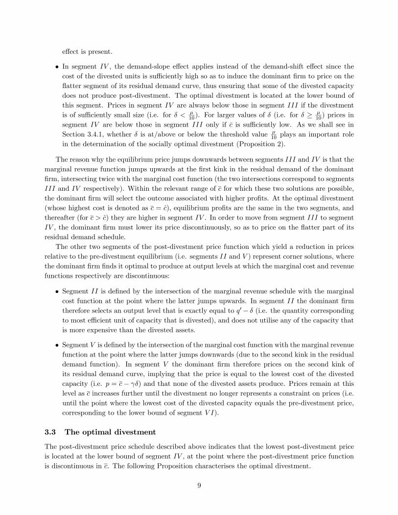
e¤ect is present.

� In segment IV , the demand-slope e¤ect applies instead of the demand-shift e¤ect since thecost of the divested units is su¢ ciently high so as to induce the dominant �rm to price on the�atter segment of its residual demand curve, thus ensuring that some of the divested capacitydoes not produce post-divestment. The optimal divestment is located at the lower bound ofthis segment. Prices in segment IV are always below those in segment III if the divestmentis of su¢ ciently small size (i.e. for � < �

10). For larger values of � (i.e. for � ��10) prices in

segment IV are below those in segment III only if �c is su¢ ciently low. As we shall see inSection 3.4.1, whether � is at/above or below the threshold value �

10 plays an important rolein the determination of the socially optimal divestment (Proposition 2).

The reason why the equilibrium price jumps downwards between segments III and IV is that themarginal revenue function jumps upwards at the �rst kink in the residual demand of the dominant�rm, intersecting twice with the marginal cost function (the two intersections correspond to segmentsIII and IV respectively). Within the relevant range of c for which these two solutions are possible,the dominant �rm will select the outcome associated with higher pro�ts. At the optimal divestment(whose highest cost is denoted as c = c), equilibrium pro�ts are the same in the two segments, andthereafter (for c > c) they are higher in segment IV . In order to move from segment III to segmentIV , the dominant �rm must lower its price discontinuously, so as to price on the �atter part of itsresidual demand schedule.

The other two segments of the post-divestment price function which yield a reduction in pricesrelative to the pre-divestment equilibrium (i.e. segments II and V ) represent corner solutions, wherethe dominant �rm �nds it optimal to produce at output levels at which the marginal cost and revenuefunctions respectively are discontinuous:

� Segment II is de�ned by the intersection of the marginal revenue schedule with the marginalcost function at the point where the latter jumps upwards. In segment II the dominant �rmtherefore selects an output level that is exactly equal to q0� � (i.e. the quantity correspondingto most e¢ cient unit of capacity that is divested), and does not utilise any of the capacity thatis more expensive than the divested assets.

� Segment V is de�ned by the intersection of the marginal cost function with the marginal revenuefunction at the point where the latter jumps downwards (due to the second kink in the residualdemand function). In segment V the dominant �rm therefore prices on the second kink ofits residual demand curve, implying that the price is equal to the lowest cost of the divestedcapacity (i.e. p = c� �) and that none of the divested assets produce. Prices remain at thislevel as c increases further until the divestment no longer represents a constraint on prices (i.e.until the point where the lowest cost of the divested capacity equals the pre-divestment price,corresponding to the lower bound of segment V I).

3.3 The optimal divestment

The post-divestment price schedule described above indicates that the lowest post-divestment priceis located at the lower bound of segment IV , at the point where the post-divestment price functionis discontinuous in c. The following Proposition characterises the optimal divestment.

9

Proposition 1 (Optimal divestment) The optimal divestment is obtained by setting c = c � �2p63 � 1

�(�� �) . This divestment has the following key features:

� it includes only capacity that the dominant �rm withholds from the market in the pre-divestmentequilibrium;

� it is located between the competitive and the pre-divestment price, that is: c 2 (pc; p�); and

� it induces the dominant �rm to price on the �atter segment of its post-divestment residual de-mand function, implying that the cost range of the divestment encompasses the post-divestmentprice, i.e. p (c) 2 (c� �; c).

The price which results with the optimal divestment is given by p (c) =p64 (�� �). For � = �

H

we have that p (c) = pc, otherwise p (c) 2 (pc; p�).

Proposition 1 establishes that the optimal divestment includes capacity that the dominant �rmis withholding from the market in the pre-divestment equilibrium, and that becomes price-settingpost-divestment. The divestment leads to the largest reduction in prices for two related reasons: (a)it does not include capacity that the generator was using pre-divestment, and it therefore does notincrease its cost relative to the pre-divestment equilibrium; and (b) it ensures that at the margin thedominant �rm faces a �atter residual demand curve (relative to the pre-divestment situation). Thelatter e¤ect induces the �rm to drop its price in order to capture more output from the competitivefringe, and prevent some of the divested capacity from producing. Only at the lower bound of therange of � that we consider (i.e. for � = �L), the optimal divestment is such that none of thedivested capacity produces and the price therefore equals the lowest cost of the divested capacity(i.e. p (c (�)) = c (�)� �L).11

As described in Proposition 1, the cost of the optimal asset divestment takes an intermediatevalue. The highest cost of the optimally divested capacity is below the pre-divestment price, meaningthat the divestment needs to be su¢ ciently competitive to be e¤ective. The optimal divestmenthowever cannot be too competitive. In particular, its highest cost needs to lie above both thecompetitive price pc (as stated in the Proposition), and the highest cost of the most e¢ cient capacityof size � not utilised by the dominant �rm in the pre�divestment equilibrium (i.e. c >

��3 + �

�).

Only if the size of the divestment is su¢ ciently large (i.e. at � = �H) the optimal divestmentcorresponds to the lowest-cost capacity of size � that is withheld by the dominant �rm pre-divestment.In this case, the optimal divestment also achieves the competitive price.12

Cheaper divestments than the optimal divestment have a lower pro-competitive e¤ect becausethe divested assets are �too e¢ cient�. This means that the price which the dominant �rm wouldneed to set to prevent some of the divested capacity from producing is too low. The dominant �rmtherefore �nds it optimal to set a higher price and su¤er a larger reduction of its residual demand(as in segment III of the post-divestment price function). As the cost of the divested capacity fallsfurther (as in segment I) divestments become even less e¤ective, since they involve capacity that thedominant �rm was already using pre-divestment. The sale of this capacity increases the cost of thedominant �rm, further reducing its incentives to drop its prices.

11 In Federico and López (2009) we show that this result also holds for all values of � less than �L:12These results also extend to � 2 (�H ; �

2), as shown in Federico and López (2009).

10

More expensive divestments than the optimal divestment are also less e¤ective because theyinvolve ine¢ cient capacity which exercises a weaker constraint on the dominant �rm. If the cost ofthe divested assets are too high, the divestment is completely ine¤ective in reducing prices (as insegment V I of the post-divestment price function).

The di¤erence in the price impact of di¤erent divestments can be signi�cant, as we illustratein Section 4 of the paper in the discussion of virtual divestments (which are at best equivalent todivestments of low-cost assets, as it is shown below).

Our results on the location and e¤ects of the optimal divestment depend on the combination ofstraightforward economic e¤ects on the pricing incentives faced by the dominant �rm, namely theabsence of an increase in its costs due to the asset sale, and the fact that the costs of the divestmentare such that the dominant �rm face a �atter residual demand at the margin. These e¤ects are robustto variations in the simplifying assumptions adopted in our baseline model, including the fact thatthe marginal cost schedule of the dominant �rm and of the fringe is symmetric, and that demand isprice inelastic. This is illustrated in Section 5, by reference to a more general model of divestments.

3.4 Impact of outright divestments on e¢ ciency and on pro�ts

Our analysis so far has centered on the impact of divestments on consumer surplus, since regulatorsand competition authorities typically focus on this welfare measure. In this section of the paper, weextend the results of our baseline model also to total welfare and industry pro�ts.

3.4.1 E¢ ciency

Our assumption of perfectly inelastic demand implies that in the baseline case divestments increaseaggregate welfare if they reduce the total costs of producing the �xed level of output �. A divestmentcan a¤ect total costs through three distinct output e¤ects, relative to the pre-divestment equilibrium:(i) a reduction in the output of high-cost capacity owned by the fringe; (ii) a change in the outputof the divested capacity; and (iii) a change in the net output of the dominant �rm (i.e. its outputnet of any fraction of the divested capacity which was being utilised by the dominant �rm in thepre-divestment equilibrium).13

The following Proposition summarises the properties of the socially optimal divestment.

Proposition 2 (Welfare) There is a threshold value of � (de�ned as �W < �H) above which theoptimal divestment from the point of view of consumer surplus coincides with the socially optimaldivestment. For lower values of �, the costs of the socially optimal divestment can be either higher orlower than the costs of the optimal divestment from the perspective of consumer welfare. In this case,the socially optimal divestment is located either at the lower bound of segment III (for � 2 [ �10 ; �

W )),or at the lower bound of segment V (for � < �

10), depending on which of these two types of divestmentyields the lower price.

We have already established in Proposition 1 that the optimal divestment delivers the social�rst-best (i.e. a competitive price) if the divestment if su¢ ciently large (i.e. � = �H). Proposition13The assumption of increasing marginal costs implies that a su¢ cient condition for price-reducing divestments to

be welfare-increasing is that the net output of the dominant �rm does not decrease post-divestment. This condition issatis�ed in all segments of the post-divestment price function but for segment III. The welfare e¤ects of a divestmentlocated in this segment are ambiguous, as it is shown in Federico and López (2009).

11

2 extends this result by showing that as long as the divestment size is su¢ ciently close to �H , theoptimal intervention from the perspective of social and consumer welfare coincide. In the baselinecase we obtain that this is the case for � � �W � 0:16�.

For lower values of � however the optimal divestment in terms of consumer welfare does notmaximise e¢ ciency because it leads to relatively high-cost divested capacity producing in equilibrium.Productive e¢ ciency is enhanced either if more expensive capacity is divested, so that none of itproduces in equilibrium, whilst still achieving a price reduction (as at the lower bound of segmentV of the post-divestment price function); or if instead cheaper capacity is sold, implying that allthe divested assets produce post-divestment, whilst ensuring that the net output of the dominant�rm does not fall (as at the lower bound of segment III). The relative impact on e¢ ciency betweenthese two alternatives is determined by their respective impact on price. This is in turn a functionof whether the size of the divestment is greater than the threshold value �

10 (as set out in Section3.2). For � su¢ ciently low (i.e. � < �

10) we obtain that a divestment located at the lower bound ofsegment V (i.e. involving high-cost assets) leads to lower price than in segment III and is thereforethe socially optimal intervention. For intermediate values of � (i.e. � 2 [ �10 ; �

W )) we obtain insteadthat selling lower cost assets located at the lower bound of segment III results in lower prices thanin segment V and a more e¢ cient outcome. Our results also imply that the divestment of low-costnon-strategic assets (located in segment I) never represents the most socially e¢ cient measure.

3.4.2 Pro�ts

We can derive the impact of a divestment on industry pro�ts from our results on prices and consumerwelfare. In doing so, we also consider the impact of divestments on the distribution of pro�tsbetween the dominant �rm and the competitive fringe. In order to study this issue, we assume thatdivested assets are sold to the fringe through a competitive tender process, so that the dominant �rmreceives the pro�ts earned by the divested assets at the post-divestment prices and quantities. Thisassumption broadly re�ects how divestments are implemented in practice in the context of antitrustcases. Our results on the impact of divestments on pro�ts are summarised in the corollary below(with additional results contained in Appendix A.4).

Corollary 1 Any price-reducing divestment leads to a fall in industry pro�ts. Both the dominant�rm and the competitive fringe prefer a high-cost divestment with a limited price impact, if the cost ofthe divested capacity is above a threshold value located within segment V of the post-divestment pricefunction su¢ ciently high (i.e. for �c > 2

3 (�+�)). For values of �c lower than this threshold value, thenthe preferred divestment from the point of view of industry pro�ts includes instead low-cost assetslocated in segment I of the post-divestment price function.

This Corollary indicates that aggregate industry pro�ts fall following a divestment that includessu¢ ciently competitive assets and which therefore is e¤ective in reducing prices. Moreover, underour assumption that the divested capacity is sold by the dominant �rm to the fringe through acompetitive auction, then the preferences of the dominant �rm and of the competitive fringe withrespect to the type of divestment are generally aligned.

The fringe always su¤ers from a reduction in price due to a divestment, since this leads to aloss of both infra-marginal pro�ts and of pro�ts on the capacity displaced by the divestment. Thelosses incurred by the fringe are proportional to the price e¤ect of divestment. This means that

12

for an intervention of a given size, the competitive fringe prefers asset divestments whose costsare su¢ ciently high and that are therefore ine¤ective. If more competitive divestments are selectedinstead, then the competitive fringe gains from the choice of e¢ cient but non-strategic assets, relativeto less competitive capacity.

The dominant �rm too always loses out from a divestment of its assets, by construction (otherwise,it would be able to realise any pro�t gain also pre-divestment). In order to reduce the pro�t loss froma divestment, the dominant �rm too prefers the sale of assets associated with a relatively limitedimpact on prices (i.e. divestments located in segments I and V ). For this type of divestments, thelosses su¤ered by the dominant �rm are proportional to the price e¤ect of the divestment, implyingthat preference of the dominant �rm on the position of the divested capacity are aligned with thatof the fringe. These results indicate that a �coalition�of the dominant �rm and its competitors maylobby for types of divestments that do not bene�t consumers.

4 Virtual divestments in the baseline case

In this section we describe the impact of virtual divestments on prices and welfare in the baselinemodel. Virtual divestments in the form of VPP schemes have been used by regulators and competitionauthorities in a number of European electricity markets to reduce e¤ective concentration. Suchschemes are often structured as a set of contract obligations on some electricity producers, wherebythese producers must pay to the holders of the contracts any positive di¤erence between the spotprice and the contract strike price, for the quantity speci�ed in the contract (like in a one-way calloption). The quantity and strike prices associated with the contracts are typically exogenous, andset by a regulator. Virtual divestments can include di¤erent type of contracts, depending on thestrike prices that are chosen, and the time periods during which the options can be exercised.14 Theoption contracts are typically sold to the market in periodic auctions, which determine the optionfee that is payable to producers for the contract(s). Our modelling of virtual divestments is directlyrelevant to the use of VPPs in electricity markets or energy release programs in gas markets15, butalso applies to the impact of �nancial contracts relative to outright divestments which is a questionof broader interest.

In what follows we model virtual divestments �exibly, allowing option contracts to have di¤erentstrike prices. For example, the strike prices of the virtual divestment may be set so as to mimic theactual cost structure of the �rm that is subject to the contract. This however does not have to bethe case, and our set-up allows us to also consider simpler contracts (e.g. a group of call options witha constant strike price), or more complex ones (with strike prices that do not necessarily correspondto production costs).

We abstract from some of potential institutional advantages associated with virtual divestmentsrelative to divestments (e.g. relating to ease of implementation and reversibility). The formalresults that we present in what follows can be therefore interpreted as providing an illustration ofthe drawback associated with virtual divestments in terms of weaker market power mitigation, and

14For example in Spain both baseload and peak VPPs have been imposed on incumbent generators between 2007and 2010. The baseload VPP applied to all hours of a given period, whilst the peak VPP could only be exercised onweek-days, between 8 am and midnight. The baseload VPP had a lower strike price than the peak VPP.15For a survey of the application of VPPs in the energy sector see Ausubel and Cramton (2010).

13

of the corresponding institutional advantages that should be associated with VPPs to justify theiradoption.

We formally de�ne a virtual divestment as a set of one or more one-way call option contracts.Each option contract j is de�ned by the pair (�j ; fj) and commits the producer subject to the virtualdivestment to pay any positive di¤erence between the market price p and an exogenously-set strikeprice fj to the holder of the option, for the quantity �j speci�ed in the contract. An option isexercised (i.e. the holder demands a payment from the producer) only if p > fj .

Suppose that there exist n � 1 contracts. Letting � be the set of the n contracts orderedfrom the lowest to the highest strike price, we have that � = f(f1; �1); (f2; �2); :::; (fn; �n)g, withf1 � f2 � ::: � fn. By de�nition, if p > fn the n options will be exercised. If instead p � fn, only asubset of options will be exercised.

The equilibrium spot price for a given virtual divestment � is de�ned as p� (�; �), where � =Pnj=1 �i. As for the case of outright divestments, we denote � as the size of the virtual divestment.

Note that if all the options are exercised (i.e. fn < p� (�; �)), the virtual divestment acts like aforward contract of size �.

4.1 Prices with virtual divestments

The following Proposition describes the impact of a virtual divestment on prices in the baselinemodel.

Proposition 3 (Virtual divestments) The largest price reduction achieved by a virtual divest-ment of size � equals �p � �

3 . This is the same impact on price as the one achieved by a low-costoutright divestment of size �. This price e¤ect is achieved if the highest strike price in the virtualdivestment scheme lies below the post-divestment price (i.e. fn < p���p). This implies that all theoptions in the virtual divestment are exercised, so that it acts like a forward contract of size �.

The reason why a virtual divestment whose options are all exercised leads to a reduction in pricesis well-known from the existing literature on forward contracts. Prices fall when a forward contractis imposed on a dominant producer due to the fact that the contract �sterilises�part of the revenuesof the dominant �rm, making them independent of the market price. Formally, this leads to anoutwards shift in the marginal revenue function of the dominant �rm, due to the fact that less ofits infra-marginal output receives the market price, so that a price reduction becomes less costly forthe �rm. This in turn leads to an output increase for the dominant �rm, along its pre-divestmentmarginal cost function, and consequently a price reduction.

A forward contract yields the same price as a low-cost outright divestment of the same sizebecause it e¤ectively removes an amount � from the infra-marginal capacity of the dominant �rm.It is as if the dominant �rm �reserves� this part of its infra-marginal assets to meet its contractobligations, foregoing the market pro�ts earned by this capacity. This is equivalent to simply notowning � units of capacity and not being subject to the contract obligation, as in the case of alow-cost divestment of size � to a competitive fringe.

Following essentially the same reasoning, it can be shown that the equivalence between thedivestment of low-cost assets to a competitive fringe and a forward contract of the same size alsoholds in oligopoly models (e.g. in Cournot, or a linear supply function model such as the one

14

considered by Green, 1999). This equivalence relies on the assumption that divested assets aretransferred to a �rm with no or insigni�cant market power (which therefore o¤ers the assets atcost, without withholding any other capacity that it may own). If instead the low-cost assets aretransferred to a �rm with some market power, then a divestment will be less e¤ective in moderatingprices relative to a forward contract (assuming that the �nancial instrument is held by �rms with nophysical assets, e.g. traders). This will not necessarily be the case for divestments of price-settingassets, on the basis of the results on outright divestments presented above.

The impact of a virtual divestment does not depend on the distribution of strike prices, as longas the highest strike price set in the contract fn lies below p���p. When some strike prices lie abovep� ��p, then it is not pro�table to exercise some of the options in the virtual divestment. This inturn results in a larger share of the output for the dominant �rm bene�tting from the market price,inducing it to set a higher price (relative to a forward contract). The optimal virtual divestmentfrom the perspective of maximising consumer welfare corresponds therefore to a set of call optionswith low strike prices, acting like a forward contract.

4.2 Comparison between the virtual divestments and outright divestments

4.2.1 Prices

Proposition 3 implies that optimal virtual divestments are never more e¤ective than optimal physicaldivestments in reducing prices. To explicitly compare the maximum price impact achieved by bothinterventions we de�ne a function R

���

�, which measures the ratio between the price reductions

achieved by the optimal divestment and by the optimal virtual divestment (that is, R = p��p(c)�p

).Given that the price reduction achieved by the optimal virtual divestment is proportional to �, thefunction R also describes the size of the virtual divestment required to match the price reductionachieved by an optimal divestment of size �, expressed as a ratio of �.

From the results obtained so far we can derive that R = 3p64 +

�2� 3

p64

��� . This function is

decreasing in �� , and ranges between 9:9 and 2:7 for � 2 (�

L; �H ]. Exploiting the results for � � �L and� 2

��H ; �2

�that are derived in Federico and López (2009)16 we can also show that R is continuous

and decreasing for all values of � between 0 and �2 , and that it equals 1 for � =

�2 . The latter result

indicates that a virtual divestment is as e¤ective as the optimal outright divestment only in the caseof very large asset sales (equivalent to the competitive output level of the dominant �rm).

The results captured by the function R shows that there is a potentially signi�cant quantitativedi¤erence in the e¤ectiveness of outright and virtual divestments as a market power mitigationmeasure. The reason for this di¤erence is that a virtual divestment only a¤ects the compositionof the revenues obtained by the dominant �rm, but cannot be used to increase the productioncapacity that is available to competitors of the dominant producer, in particular by targeting assetsthat the dominant �rm would otherwise withhold from the market. Unlike the optimal outrightdivestment, a virtual divestment cannot increase the competitive pressure faced by a dominant �rmat the margin, by increasing the output available to competitors. A further implication of this resultis that mimicking the properties of the optimal divestment by setting a range for the strike prices inthe virtual divestment that is similar to the cost range of the optimal divestment does not increase

16For � 2 (0; �L] we have that R���

�=p2��� 1. For � 2 (�H ; �

2] we have that R

���

�= 1

2��.

15

the pro-competitive impact of the virtual divestment.17

4.2.2 E¢ ciency and pro�ts

The optimal virtual divestment is welfare-increasing, since it induces the dominant �rm to increase itsoutput, thus leading to a reduction in the output of high-cost capacity belonging to the competitivefringe. However, the optimal outright divestment always leads to a greater e¢ ciency increase thanthe optimal virtual contract, as stated in the following Proposition.

Proposition 4 Optimal divestments increase total welfare by more than the optimal virtual divest-ment of the same size.

This Proposition implies that outright divestments, if chosen optimally, can increase both con-sumer welfare and e¢ ciency by more than virtual divestments. The intuition for the e¢ ciency resultis that at the optimal divestment a greater fraction of the production of the competitive fringe shiftsfrom high-cost assets to lower cost capacity (i.e. that which is divested), coupled with the fact thatthe dominant �rm also increases its net output (for � < �H). This e¢ cient reallocation of outputtakes place to a greater extent than with a virtual divestment, since the latter yields a lower reductionin prices. These e¤ects outweigh the ine¢ ciency associated with production by relative expensivedivested capacity under the optimal outright divestment.

Our earlier results on the impact of pro�ts of an outright divestment also imply that producerswill jointly and individually prefer a virtual divestment to a physical one, unless the costs of theassets chosen to be divested are su¢ ciently high.

5 Robustness of results

The results presented so far on the impact of di¤erent types of divestments on price (and the relatedresults on virtual divestments) rely on standard economic e¤ects. These e¤ects can naturally beexpected to apply also in a more general model than the baseline framework that we employed abovefor expositional clarity.

In order to generalise our baseline model we assume that the cost schedules of the dominant �rmand the fringe can have di¤erent slopes, denoted as i for i = d; f . We also assume that the overalldemand schedule is price-elastic, with slope �, so that qd+ qf = ���p. It is straightforward to showthat in such a general model the pre-divestment price p� equals 1+ dx

2+ dx�x (where x = � + 1

f), and

that the pre-divestment output of the dominant �rm q�d equals�

2+ dx.

Following the same methodology used for the baseline model, we can identify a unique optimaldivestment, for an intermediate range of the size of the divestment �, and can compare its priceimpact with that of other types of divestment, including in particular the sale of low-cost assets.Under the more general assumptions, the optimal divestment still includes capacity that the domi-nant �rm withholds pre-divestment, and that is price-setting post-divestment. Furthermore, virtual

17A virtual divestment that is explicitly designed to mimic the optimal divestment (i.e. with a maximum strikeprice equal to c, and a strike price function with the same slope as the marginal cost function of the dominant �rm)is actually equivalent to a forward contract, and therefore remains less e¤ective than the optimal divestment. Thisfollows from the fact that c < p� ��p.

16

divestments remain equivalent to the outright sale of low-cost assets. These analytical results aresummarised in Appendix A.7.18

Appendix A.8 illustrates the results of the more general model by means of a simple numericalexample. This example con�rms that the main results of the analytical model are robust to variationsin the cost parameters of the competing �rms and in the demand slope parameter. In particular,the optimal divestment is still intermediate with respect to its location on the cost function of thedominant �rm. Comparative statics can also be derived by means of the numerical example. Inparticular, we observe that as the costs of the dominant �rm increase relative to the fringe or thedemand slope parameter increases, the position of the optimal divestment converges to the cost of themost competitive capacity of size � withheld by the dominant �rm in the pre-divestment equilibrium.

6 Conclusion

This paper has studied the impact of remedy design in a model where a dominant producer facesa competitive fringe. We analysed the e¤ect on market prices, e¢ ciency and pro�ts of transfers ofcapacity from a dominant producer to a competitive fringe. We show that divesting capacity withintermediate costs can be several-fold more e¤ective in reducing prices that an equivalent transferof low-cost assets. In order to maximise the e¤ectiveness of the divestment in reducing prices, thedivested capacity needs to include assets which are su¢ ciently competitive to impose a competitiveconstraint on the dominant �rm but whose costs are not too low so as to induce the dominant producerto accept a larger loss of its output post-divestment in order to keep prices high. In the optimal post-divestment equilibrium, the cost range of the divested capacity needs to span the post-divestmentprice (implying that some but not all of the divested capacity produces in equilibrium). We also �ndthat the optimal divestment from the perspective of consumer welfare is always e¢ ciency-increasing,and that it coincides with the socially optimal divestment for su¢ ciently large divestments.

We have also compared the e¤ectiveness of outright asset sales to that of virtual divestments. Wehave established that the e¤ectiveness of virtual divestments is maximised when all of the optionsthat are sold are exercised, so that the remedy acts like a forward contract. Even if this is the casethe virtual divestment reduces prices only as much as a physical divestment of low-cost capacity.Our �ndings therefore imply that outright divestments can be signi�cantly more pro-competitivethan their virtual equivalent. By the same token, both the dominant �rm and the competitive fringebene�t from the imposition of a virtual divestment relative to a more e¤ective outright divestment.

Our �ndings have direct policy relevance, given that divestments are frequently accepted bycompetition authorities as commitments in competition cases. Virtual divestments are also commonlyused in the wholesale electricity sector. Our results are also applicable to the evaluation of mergere¤ects, since divestments are the opposite of a merger. The �ndings of this paper imply that a mergerwhere a larger incumbent buys strategic capacity from a smaller competitor can have signi�cantlygreater e¤ect on prices than one where additional e¢ cient capacity is purchased instead. Similarly,our results indicate that the price-increasing e¤ect of the acquisition of a given volume of low-costcapacity by a �rm with market power can be remedied by signi�cantly smaller divestments of price-setting capacity.

A possible extension of the approach presented in this paper includes the analysis of the case

18The proof of these results is available from the authors.

17

of asset divestments to new entrants or players with insigni�cant market power in the context ofoligopoly interaction between incumbent �rms. Obtaining comprehensive analytical results on theimpact of the divestments of di¤erent type of assets in standard oligopoly models for homogenousproducts (e.g. Cournot or Supply Function Equilibria) is challenging, given the discontinuities createdby asymmetric asset sales. However, some of the core results presented in this paper (in particularthe fact that the divestment of low-cost assets is ine¤ective relative to the sale of assets with highercosts, and that virtual divestments are at best equivalent to the divestment of low-cost assets) canalso be extended to oligopoly models, given the general nature of the underlying cost and demande¤ects that we identify in this paper.

References

[1] Akgün, U., 2004, �Mergers with supply functions�, Journal of Industrial Economics, 52, 535-546.

[2] Allaz, B. and J.-L. Vila, 1993, �Cournot Competition, Forward Markets and E¢ ciency�, Journalof Economic Theory, 59, 1-16.

[3] Armington, E., E. Emch and K. Heyer, 2006, �Economics at the Antitrust Division�, Review ofIndustrial Organization, 29, 305-326.

[4] Ausubel, L. and P. Cramton, 2010, �Virtual power plant auctions�, Utilities Policies, 18, 201-208.

[5] Bushnell, J., 2007, �Oligopoly Equilibria in Electricity Contract Markets�, Journal of RegulatoryEconomics, 32, 225-245.

[6] Crawford, G., J. Crespo, H. Tauchen, 2007, �Bidding asymmetries in multi-unit auctions: Im-plications of bid function equilibria in the British spot market for electricity�, InternationalJournal of Industrial Organization, 25, 1233-1268

[7] De Frutos, M.-A., and N. Fabra, 2012, �How to allocate forward contracts: the case of electricitymarkets�, European Economic Review, 56, 451-469.

[8] Federico, G. and A. L. López, 2009, �Divesting Power�, IESE Business School, Working PaperWP-812.

[9] von der Fehr, N.H. and D. Harbord, 1993, �Spot market competition in the UK electricityindustry�, Economic Journal, 103, 531-546.

[10] Gilbert, R. and D. Newbery, 2008, �Analytical Screens for Electricity Mergers�, Review ofIndustrial Organization, 32, 217-239.

[11] Green, R., 1996, �Increasing Competition in the British Electricity Spot Market�, The Journalof Industrial Economics, 44, 205-216.

[12] Green, R., 1999, �The Electricity Contract Market in England and Wales�, The Journal ofIndustrial Economics, 47, 107-124.

18

[13] Newbery, D., 1998, �Competition, Contracts and Entry in the Electricity Spot Markets�, TheRand Journal of Economics, 29, 726-749.

[14] Schultz, C., 2009, �Virtual Capacity and Competition�, mimeo.

[15] Vergé, T., 2010, "Horizontal mergers, structural remedies, and consumer welfare in a Cournotoligopoly with assets", The Journal of Industrial Economics, 58, 723-741.

[16] Willems, B., 2006, �Virtual Divestitures, Will they make a Di¤erence?: Cournot Competition,Options Markets and E¢ ciency�, CSEM WP 150.

[17] Wolak, F. and S. McRae, 2008, �Merger Analysis in Restructured Electricity Supply Industries:The Proposed PSEG and Exelon Merger (2006)�, in J. Kwoka and L. White (eds.), The AntitrustRevolution: Economics, Competition and Policy, Oxford University Press.

19

Appendix A

A.1 The post-divestment price function

Table 1: The post-divestment price function

Segment Price Range of cI p� ��p � � c < p�

2 +�p

II �� c p�

2 +�p � c <p�

2 + 2�p

III p� � 2�p p�

2 + 2�p � c < cIV 3

8( (�� �) + c) c � c < (35�+ �)V c� � (35�+ �) � c < p

� + 3�pVI p� c � p� + 3�p

;

where p� = 23 �; �p �

�3 ; and c �

�2p63 � 1

�(�� �).

A.2 Proof of Proposition 1

This Proposition assumes that � 2��1� 12

5p6

��;�1� 2p

6

��i, which we denote as � 2

��L; �H

�.

The dominant �rm�s post-divestment marginal cost is de�ned by the following two-step function:

cd =

( qd if qd < q

0 � � (qd + �) if qd � q0 � �

,

where the �rst step corresponds to the pre-divestment cost function, whilst the second step corre-sponds to the cost-increasing e¤ect of divestments described in the main text.

The competitive fringe�s post-divestment marginal cost function (which is equivalent to the inverseresidual demand of the dominant �rm) is de�ned by the following three-step function:

cf =

8><>: (�� qd � �) if qd < �� q0 � �

2 (�+ q

0 � qd � �) if �� q0 � � � qd � �� q0 + � (�� qd) if qd > �� q0 + �

.

where the �rst step corresponds to the demand-shift e¤ect described in the main text, the secondto the demand-slope e¤ect, and the third coincides with the pre-divestment case.

As the model is discontinuous we have to study the �rm�s maximization problem in each ofthe regions de�ned by q0 (for a given �), in order to derive the post-divestment price function andidentify the optimal divestment. This proof proceeds in three parts. First, we identify the fourinterior solutions that exist to the �rm�s maximisation problem. A unique candidate equilibrium canexist inside each region of q0 since the model is linear. Second, we study equilibria at the regionswhere the feasibility conditions for the interior solutions are not satis�ed. Third, we identify thelevel of q0 at which post-divestment prices are minimised. The various candidate equilibrium casesthat we identify in this proof are illustrated in Figure 3.

20

Interior solutions

Case I (low-cost divestment): in this region the dominant �rm and the competitive fringe of�rms produce, respectively, at a higher and lower marginal cost than in the pre-divestment case, i.e.,cd = (qd+ �) and cf = (�� qd� �). The dominant �rm maximises �Id = p

IqId � 2 (q

Id)2� �qId with

respect to qId and subject to pI = cf , which yields qId = q

�d � 2

3�. This implies that pI = p�� �

3 . Thetwo feasibility conditions for this equilibrium are qId < �� q0 � � and qId � q0 � �. These conditionsreduce to the following expression:

Case I: pI = p� � �3for q0 � �+ �

3.

Case III: the dominant �rm produces at the pre-divestment marginal cost, while the competitivefringe produces at a lower marginal cost, i.e., cd = qd and cf = (��qd��). Thus, pIII = (��qd��)and �IIId = pIIIqIIId �

2 (qIIId )2. The �rst-order condition yields qIIId = q�d � �

3 , implying thatpIII = p� � 2 �

3 . The feasibility conditions are qIIId < �� q0 � � and qIIId < q0 � �, which boils down

to the following expression:

Case III: pIII = p� � 2 �3for

�+ 2�

3< q0 <

2(�� �)3

.

Case IV : the dominant �rm produces at the pre-divestment marginal cost, while the competitivefringe produces at the �atter part of its marginal cost function, i.e., cd = qd and cf =

2 (�+q

0�qd��).Thus, pIV =

2 (�+q0�qd��) and �IVd = pIV qIVd �

2 (qIVd )2. From the �rst-order condition we obtain

qIVd = �+q0��4 , and pIV = 3

8( (�� �) + c). The feasibility conditions can be expressed as follows:

Case IV : pIV =3

8( (�� �) + c) for

(35(�� �) � q

0 � 35�+ � if � � �

6

� + �3 < q

0 � 35�+ � if � > �

6

.

Case V I: the dominant �rm and the competitive fringe of �rms produce at the pre-divestmentmarginal cost, so that the equilibrium is the same as the pre-divestment outcome. Here, the feasibilityconditions imply the following:

Case V I: pV I = p� for q0 >2

3�+ �.

Overlap between Case III and Case IV . Cases III and IV always overlap since � + �3 <

23(� � �) for � <

�5 (which is the case in the range of � that we consider), and

35(� � �) <

23(� � �)

(which de�ne the respective regions for � � �6 ). The overlap between these two interior solutions

occurs because the marginal revenue schedule of the dominant �rm jumps upwards at the �rst kink inthe post-divestment residual demand curve, crossing the marginal cost schedule twice. In the overlapregion the dominant �rm will choose the equilibrium associated with the highest pro�ts. From theexpressions for pro�ts derived above note that �IIId does not depend on the value of q0 whilst �IVdis increasing in q0 (as we show formally below). We can therefore identify an indi¤erence value forq0 (de�ned as q) such that, for q0 < q we have �IIId > �IVd (i.e. Case III represents the equilibriumoutcome), and for q0 > q Case IV is the equilibrium.

From the equilibrium prices and quantities given above, we can compute that �IIId = 6 (�� �)

2,and �IVd =

16 (�� � + q0)2. The pro�t-indi¤erence point q is therefore given by the following

21

quadratic condition (obtained by simplifying the two expressions for pro�ts ): (���)23 = (���+q0)2

8 .This yields a unique positive root in q0 given by:

q0 =

2p6

3� 1!(�� �) � 0:63 (�� �) .

We therefore de�ne q ��2p63 � 1

�(�� �). As we discuss in the main text, this identi�es the

optimal divestment policy for the range of � considered in this Proposition. Note that c(q) = q � cis below p�, as should be expected. We also have that c > pc (as stated in the Proposition) as longas � < 4

p6�9

4p6�6�, which is satis�ed in the relevant range of �.

For q0 = q to be consistent with Case IV it needs to be contained within the range of q0 thatde�nes Case IV: This implies the following two conditions on �:

q <3

5�+ � ) � >

�1� 12

5p6

�� � �L,

q � �

3+ � (for � >

�

6)) � �

�1� 2p

6

�� � �H .

The two resulting conditions on � are assumed to hold in this Proposition, and de�ne the rangeof intermediate divestments.

Corner solutions

Case II. For �+�3 � q0 < �+2�3 the interior solutions identi�ed in Cases I; III; IV and V I are not

feasible. In this region of q0 we have that the �rst segment of the marginal revenue curve passesthrough the jump of the marginal cost curve, at qd = q0 � �. The dominant �rm does not haveincentive to produce more or less than q0 � �, since the corresponding interior equilibria are notfeasible. Thus, in this region the dominant �rm �nds it optimal to set qIId = q0 � �, implying thatpII = (�� q0). We therefore have:

Case II: pII = (�� q0) for �+ �3

� q0 < �+ 2�

3.

Case V . For 35� + � < q

0 < 23� + � we have that the interior solutions of Cases I; IV and V I

are not feasible, and that Case III is feasible only for � < �25 .

� We consider �rst the case where � � �25 . In this case, none of the interior solutions are feasible,

because the marginal cost curve crosses the second (downwards) jump of the marginal revenuecurve. It is therefore optimal for the dominant �rm to price at the second kink of its residualdemand curve, setting pV = (q0� �) = c� �. This is an equilibrium as long as pV < pV I (i.e.q0 < 2

3�+ �).

� If � < �25 , Cases III and V overlap (for 35� + � < q

0 < 23(� � �)). If this is the case we have

that pro�ts in Case V are higher than those in Case III, and Case V therefore representsthe post-divestment equilibrium. This follows from the fact that at the lower bound of therelevant range of q0 (i.e. q0 = 3

5� + �), we have that pro�ts in Cases IV and V are equal(since the two cases are the same) and that pro�ts in Case IV are higher than those in Case

22

3δµ +

32δµ +

( )δµµδ −≤53:

6if

δµµ

δ +≥53:

25if

( )δµ −32

δµµδ +<53:

25if

δµ +32

Case I Case IICase III

Case IV

3:

6µ

δµ

δ +>if

Case V

Case VI

q’3

δµ +32δµ +

( )δµµδ −≤53:

6if

δµµ

δ +≥53:

25if

( )δµ −32

δµµδ +<53:

25if

δµ +32

Case I Case IICase III

Case IV

3:

6µ

δµ

δ +>if

Case V

Case VI

q’

Figure 3: Summary of segments of the post-divestment price function.

III (since 35� + � > q). We also have that �Vd increases with q

0 (because higher values of q0

imply that the kink on the residual demand curve on which the dominant �rm is pricing isassociated with a higher price level). Since �IIId is constant in q0, it follows that �Vd > �

IIId for

35�+ � < q

0 < 23(�� �).

We therefore have:

Case V : pV = c� � for 35�+ � < q0 <

2

3�+ �.

Price comparison

The minimum pII is achieved at q0 = �+2�3 , where pII = p� � 2

3 � = pIII . Therefore, for any level

of �, we have the following price ranking: pIII = min pII < pI < pV I = p�. The minimum pV isachieved at q0 = 3

5�+ �, where pV = 3

5 �. The price corresponding to Case IV equals the minimumpV for q0 = 3

5�+�, and takes a lower value for q0 < 3

5�+� (since it is increasing in q0). Note also that

the price set by the dominant �rm at the point where the pro�ts associated to Cases III and IV areequal is necessarily lower in Case IV than in Case III. The reason is that when the �rm deviatesto Case IV it prices on the �at part of its residual demand curve, moving away from pricing on thesegment of the residual demand curve located to the left of the �rst kink. In order to do so it mustexpand output. From the above it follows that the lowest price is achieved when the divestment islocated at the indi¤erence point between Case III and Case IV; that is c = q �

�2p63 � 1

�(�� �).

The price at this point can be computed as p(c) =p64 (�� �). The output of the dominant �rm at

the optimal divestment is given by qIVd = �+q��4 = ���p

6� �

3 .

A.3 Proof of Proposition 2

This proof relies on the fact that the change in welfare from a divestment can be expressed as thechange of total production costs due to the three output e¤ects described in the main text: (1)the reduction in output of high-cost capacity owned by the fringe; (2) the change in output of the

23

divested capacity; and (3) the change in the output of the dominant �rm net of the pre-divestmentoutput of the divested assets. We denote as �W j the change in welfare obtained in each range j ofthe position of the divested capacity, as de�ned by the post-divestment price function, and �W

jas

the maximal change in any given range. To compute welfare, we also rely on the post-divestmentequilibrium price and output levels obtained in the proof of Proposition 1.

Case I. In this case only the �rst two output e¤ects described above apply, and we have that

�W I =

Z 23�

2���3

xdx�Z �+�

3

�3

xdx = �9 (�� �).

Case II. As in the previous case, only the �rst two output e¤ects apply, so that we have

�W II =

Z 23�

��q0 xdx�

R q0�3 xdx =

2

��49�

2 � 2 (q0)2 + 2�q0�. Notice that @�W II=@q0 > 0 provided

that � < �4 . Therefore welfare is maximised at the upper boundary of segment II (i.e. q

0 = �+2�3 ),

where we have that �WII= 2 �

9 (�� 2�) (where the upper bar indicates the maximum welfareachieved in a given case).

Case III. All three output e¤ects are relevant here, and we have that �W III =R 23�

23(���) xdx+Z �

3

���3

xdx �Z q0

q0�� xdx = �

�29� +

59�� q

0�. Hence @�W III=@q0 < 0, so that total welfare is

maximised at the lower boundary of the relevant range of q0 (i.e. q0 = �+2�3 ), where �W

III

= �WII= 2 �

9 (�� 2�).Case IV: All three output e¤ects also apply in this case, and we have that:

�W IV =

Z 23�

38(���+q0)

xdx�Z 3

8(���+q0)

q0�� xdx�

Z ���+q04

�3

xdx

=

2

�61

288�2 +

11

16�� � 11

16�q0 +

21

32�2 � 21

16�q0 +

21

32

�q0�2� .

This expression shows that @�W IV =@q0 is linear in q0 but that its sign is ambiguous (i.e. @�W IV =@q0 <

0 only if q0 < 1121�+ �). Therefore, there exist two possible e¢ ciency-maximising points: one located

at its lower boundary q0 =�2p63 � 1

�(�� �); and one at its upper boundary q0 = 3

5�+ �.Case V . In this case we have that only the �rst and third output e¤ect apply, since the divested

capacity does not produce in equilibrium. We therefore have that: �W V = �R ��q0+��3

xdx +R 23�

q0�� xdx = 2

��49�

2 � 2 (q0)2 � 2�2 + 4q0� � 2�� + 2�q0�.

Notice that @�W=@q0 < 0 provided that q0 > � + �2 , which holds in Segment V . Therefore,

the e¢ ciency-maximising location is at q0 = � + 35�, which in turn implies �W

V= 4

225 �2 =

�W IV��q0=�+ 3

5�:

Socially optimal divestment

First, notice that �WII= �W

III> �W I provided that � < �

3 . Let us now denote by �j�k

the di¤erence between �Wjand �W

k. We have that �III�V (�) =

�� 4225�

2 + 29�� �

49�2�. This

implies that �III�V = 0 for � = 25� (which is outside the range that we consider) and for � =

�10 . It

follows that �WIII

< �WVfor � < �

10 , given the concavity of �III�V in �.

24

To complete the proof we need to compare the highest change of welfare achieved in either caseIII or V with the one obtained under case IV for q0 =

�2p63 � 1

�(�� �) (which is one of the two

possible maxima for case IV , the other being equivalent to case V ).Consider �rst the case � < �

10 . Here we must compare case V with case IV . We have: �IV�V (�) =

��327200 �

23

p6��2 + 7

8�2 �

�74 �

23

p6����. This expression is convex in � and it equals 0 for � =�

1� 25

p6�� � �L and for � =

�1� 38

105

�� (which is above the relevant range of �). We therefore

have that �WIV< �W

V, for � 2 (�L; �10).

Consider now the case � � �10 . We must compare case III with case IV . Here we have that

�IV�III(�) = ��11972 �

23

p6��2 + 95

72�2 �

�7136 �

23

p6����, which is also convex in �. From this we

obtain that �IV�III = 0 for

� = �W � �24p6 + 71 + 6

p�78 + 32

p6

95� and � = � � �24

p6 + 71� 6

p�78 + 32

p6

95�,

where � < �10 . Therefore, for � 2 (

�10 ; �

W ), we have that �IV�III < 0, i.e., the welfare maximumcorresponds to the maximum achieved under case III. Conversely, for � � �W , we have that�W

IV> �W

III, as stated in the Proposition.

A.4 Corollary 1

Divestments that reduce market prices also reduce total industry pro�ts. Assuming that the fringepurchases the divested capacity through a competitive process, then it makes no pro�ts on thedivested assets (as these pro�ts are simply transferred to the dominant �rm), and instead su¤ersa pro�t loss on the rest of its capacity, due to the reduction in infra-marginal rents and the lossof marginal output (net of the output produced by the divested assets). The loss su¤ered by thefringe is proportional to the impact of divestments on price. The dominant �rm too loses out froma divestment, by construction (otherwise it could replicate the post-divestment outcome also pre-divestment).

Aggregate pro�ts are obviously maximised in region V I, for q0 � 23�+ �. If a more competitive

divestment is chosen instead, producers will prefer a divestment located in either region I or V . Inthese two regions, both of the dominant �rm�s and the fringe�s pro�t levels are positively correlatedwith prices. In the case of the dominant �rm this follows from the fact that in region I the loss inpro�ts is due to the reduction in price associated with an increase in the combined output of thedominant �rm and the divested capacity of �3 , along the pre-divestment cost curve. In region V , thedominant �rm expands output in order to reduce prices, and the divested assets do not produce. Thishas the same qualitative impact on the pro�ts of the dominant �rm (including those earned on thedivested assets) as that of region I, with the only di¤erence being the relative impact on prices andvolumes. The dominant �rm will therefore prefer the region associated with the smaller deviationfrom the pre-divestment optimum. The Proof of Proposition 1 further implies that the dominant�rm�s pro�ts in the other possible regions of the post-divestment price function (i.e. segments II ;III and IV ) are lower than those in regions I and V , also accounting for the pro�ts earned on thedivested capacity (which are maximised in segment I).

These results mean that producers will individually and jointly prefer the type of divestmentassociated with a higher price. We have that pI > pV if q0 < 2

3 (�+ �), so that producers will prefera divestment in region I for q0 < 2

3 (�+ �), and in region V otherwise.

25

A.5 Proof of Proposition 3

Assume �rst that all options in the virtual divestment are exercised. In this case, the pro�t of thedominant �rm is �d = pqd �

2 (qd)2 + z � p�, where z =

Pnj=1 fj�j . The �rst-order condition yields

qd =�+�3 , and therefore p = p

�� �3 (where �p �

�3 ). The feasibility conditions are that p > fn and

qd � �: The former implies: fn < p� � �3 : To satisfy the second condition we require � �

�2 (which

is within the range of intermediate divestments that we study).To show that the largest price reduction achieved by a virtual divestment equals �p, we need

to also consider the case of a set of contracts for which the dominant �rm �nds it optimal to seta price such that some options are not exercised. For a given price p such that fx � p < fn,the number of options that are exercised is de�ned as x(p). Hence the dominant�s pro�t is �d =pqd �

2 (qd)2 + z(x(p))� p�(x(p)), where z(x(p)) =

Px(p)j=1 fj�j and �(x(p)) =

Px(p)j=1 �j . The optimal

price for the dominant �rm can be found by �rst �nding the price that maximizes its pro�t functionfor each number of exercised options in isolation. And second, by comparing the pro�t in each ofthese cases. The optimal price will be given by the one that yields the maximum pro�t among allthe possible cases.

Suppose that p is such that �x options are exercised, then by maximizing �d(�x) = pqd � 2 (qd)

2 +

z(�x) � p�(�x) we �nd that p(�x) = p� � �(�x)3 and q(�x) = �+�(�x)

3 , provided that f�x+1 > p(�x) � f�x,otherwise p(�x) = f�x. Therefore, for each x 2 (1; :::; n� 1) we can construct a candidate equilibriumin which the dominant �rm�s pro�t is given by �d(p(x); q(x)). Let y be such that �d(p(y); q(y)) ��d(p(x); q(x)) holds for any x 6= y. It follows that p�(�; �) = p(y). Notice that p(y) > p� � �

3 since�(y) < �, which completes the proof of the Proposition.

A.6 Proof of Proposition 4

The results shown so far imply that welfare impact of the optimal virtual divestment is the same asthe one of a low-cost divestment situated in segment I. It is therefore equal to �

9 (�� �), as shownin the Proof of Proposition 2. Recall also that at the optimal divestment, the price and outputof the dominant �rm are respectively given by p(c) =

p64 (�� �) and q

IVd = ���p

6. These results

imply that the welfare impact of the optimal divestment from the perspective of consumers (whichwe de�ne as �W ) is given by the following expression:

�W =

23�Z

p64(���)

xdx�

���p6Z

�3

xdx�

p64(���)Z

�2p6

3�1�(���)��

xdx =

��119

72� 23

p6

��2 +

7

8�2 �

�7

4� 23

p6

���

�.

We thus have that �W � �W I = ��11972 �

23

p6��2 + 71

72�2 �

�6736 �

23

p6����. The gradient of

�W ��W I is given by 5 (�; �) =�dd�

��W ��WB

�; dd�

��W ��WB

��, with 5(0; 0) = 0. The

Hessian matrix of �W � �W I is positive de�nite. Hence, � = � = 0 is a global minimum, where�W ��W I = 0. For any positive � and �, we thus have that �W ��W I > 0.

26

A.7 Summary of results in the general case

In the general case we assume that ci = iqi for i = d; f and that qd + qf = � � �p. The residualdemand curve faced by the dominant �rm is therefore given by p = ��qd

x where x � � + 1 f. Max-

imisation of the dominant�s �rm pro�t function yields the pre-divestment price and output followingstraightforward calculations:

q�d =�

2 + dx; and p� =

1 + x

2 + x

�

x

The various segments of the post-divestment price function can be derived using the same method-ology used in the baseline model, by identifying the various steps in the post-divestment cost andresidual demand function of the dominant �rm, and establishing the feasibility conditions for eachsolution to the optimisation problem. Using this methodology we obtain the following results forlow-cost divestments (in segment I of the post-divestment price function, as de�ned in the baselinecase), and at the optimal divestment (which is located in the overlap between segments III and IV ,as in the baseline case). The corresponding proof for these results is available separately from theauthors.

Case I (low-cost and/or virtual divestment). In this case we obtain that pI = p�� �x(2+ dx)

,

which simpli�es to the baseline result for d = and x = 1 . This is the same price e¤ect that is

obtained by imposing a forward contract of size �, with a maximum strike price below pI .Optimal divestment. We �nd that the optimal divestment is located at the following point in

the cost function of the dominant �rm: bc = d �pA� 1� (�� �), whereA �

�3 f + d + � d f

� � f + d + � f d

�� d + 2 f + � d f

� �1 + � f

� d

.

Note that in the baseline case A simpli�es to 83 , so that

pA = 2

p63 . We also have that the price at

the optimal divestment equals p(bc) = pA�(�+ d)2�+ d

(�� �), where � � d f d+ f+ d f�

. For d = f =

and � = 0 we have that � = 2 , so that we obtain that p(bc) = p

64 (�� �) , con�rming the result

obtained for the baseline case.We also have that the optimal divestment is feasible for � � �H �

�1� 1p

A

�2�+ d�+ d

���, which is

the binding condition in the numerical example presented in the text (for su¢ ciently high values of d or �, and su¢ ciently low values of f ). This condition too collapses to the equivalent condition

in the baseline case (� � �H ��1� 2p

6

��) for A = 8

3 and � = 2 .

A.8 Robustness of results: numerical example

In this example we assume that � = 90, � = �10 , and (for the baseline case) d = f = 1. These

assumptions imply that in the baseline case we have a pre-divestment price of 60, a price at theoptimal divestment of 49:6 and a price following the divestment of low-cost assets (or a virtualdivestment) of 57. The ratio of the price impact of the optimal divestment and of the divestment oflow-cost assets (i.e. R) therefore equals 3:47. We also have that the position of the optimal divestmentin the baseline case equals 51:3, above both the competitive price of 45 and the corresponding post-divestment price of 49:6.

27

iγ ρiγ ρ

Figure 4: Values of R���

�as d, f or � vary, respectively shown in Panel 4.A (continuous line

(Rd)), Panel 4.A (dotted line (Rf )) and Panel 4.B.

Figure 4 illustrates the relative price impact function R as we respectively relax the assumptionof cost-symmetry (allowing each of d and f to vary between 0:6 and 1:75, keeping the other costparameter constant at 1); and the one of price-inelastic demand, allowing the demand slope parameter� to vary between 0 and 0:75.19 Both panels of the �gure illustrate the fact that in the more generalmodel the optimal divestment remains much more e¤ective than divestments of low-cost capacity inreducing prices. In the numerical example that we consider the value of the function R never fallsbelow 3:4 as the cost parameter varies, and it increases as the degree of dominance rises through areduction of the costs of the dominant �rm relative to the competitive fringe (either because of alower value for d or a higher value for f ). The value of R reaches a maximum of close to 3:9 ifthe cost of the fringe is at the upper bound of the range that we consider. The function R remainsabove a value of 3:4 also as the slope of the demand function increases, and it takes a higher valuethan in the baseline case for � su¢ ciently high.

Figure 5 plots our results on the position of the optimal divestment as the parameters of the modelvary, relative to three possible benchmarks: the pre-divestment price, the competitive price, and thecost of the most competitive capacity of size � withheld by the dominant �rm in the pre-divestmentequilibrium (recall that this benchmark takes the value of

��3 + �

�in the baseline model). For the

baseline case we established the the highest cost of the optimal divestment takes an intermediate valuethat lies below the �rst benchmark, but above the other two. This result is con�rmed in the more

19This parameter range is selected to ensure that the condition � � �H is satis�ed (so that we are in a range ofintermediate divestments). In the baseline case considered in this numerical example we have that �H = 16:51 (whichis well above the size of the divestment used for the illustration, i.e. � = �

10= 9 ). In this example we also have

that � = �H = 9 for the following parameter combinations:� d = 1:78; f = 1; � = 0

;� d = 1; f = 0:56; � = 0

;�

d = f = 1; � = 0:78:

28

dγ

ρ

fγdγ

ρ

fγ

Figure 5: Relative position of the optimal divestment, as d, f or � vary (respectively shown inPanels 5.A, 5.B and 5.C)

general model, as shown in the �gure. We �nd that as the relative costs of the dominant �rm increaserelative to the fringe (so that its pre-divestment share of the market falls, and the e¤ective size ofthe divestment increases towards �H), the position of the optimal divestment converges towards thetwo lower benchmarks described above. For � = �H the location of the optimal divestment exactlyequals the cost of the most competitive capacity withheld by the dominant �rm in the pre-divestmentequilibrium, which is the same result that we obtain in the baseline model. We obtain a similar resultas demand becomes more elastic (i.e. when � increases), as it is shown in the corresponding panelof the �gure.

29