OPTICAL SOLITONS IN QUADRATIC NONLINEAR MEDIA AND ...
88
UNIVERSITAT POLITÈCNICA DE CATALUNYA Laboratory of Photonics Electromagnetics and Photonics Engineering group Dept. of Signal Theory and Communications OPTICAL SOLITONS IN QUADRATIC NONLINEAR MEDIA AND APPLICATIONS TO ALL-OPTICAL SWITCHING AND ROUTING DEVICES Autor: María Concepción Santos Blanco Director: Lluís Torner Barcelona, january 1998
Transcript of OPTICAL SOLITONS IN QUADRATIC NONLINEAR MEDIA AND ...

UNIVERSITAT POLITÈCNICA DE CATALUNYA
Laboratory of Photonics Electromagnetics and Photonics Engineering group
Dept. of Signal Theory and Communications
OPTICAL SOLITONS IN QUADRATIC NONLINEAR MEDIA AND
APPLICATIONS TO ALL-OPTICAL SWITCHING AND ROUTING DEVICES
Autor: María Concepción Santos Blanco
Director: Lluís Torner
Barcelona, january 1998

Chapter 6
Applications to Soliton Steering
Previous chapters as primarily dealing with description of the basic features of soliton propa-
gation in %(2) structures, although often relying on numerical simulations, have mainly put the
emphasis on rather theoretical aspects aiming basically at providing a complete basic knowl-
edge of the solitary waves existing in those structures and the characteristics of their excitation.
This theoretical description has set the basis for the design of practical setups that exploit the
properties of solitary wave propagation along with those of quadratically nonlinear media. Sky
is the limit when thinking of applications in which solitary wave propagation excited with low
input powers in materials of current use in optical technology is susceptible of improving the
present state of the art in optical applications. Quadratic nonlinearities further offer the oppor-
tunity of spatial two-dimensional confinement which opens the door to a bunch of applications
to the routing and steering in bulk materials such as for example interconnection matrixes.
Optical beam steering is the issue in this Thesis and therefore, practical setups which take
advantage of the properties of solitary waves arising in x^ structures for the steering control
of optical beams will be analyzed in the present Chapter. Two-dimensional (2+1) geometries
might be more interesting from the stand point of practical applications because of the versatility
they offer and also for the greater simplicity of the setups required. However, integrated devices,
which are the ultimate goal, require (1+1) configurations. In addition to that, the primary
interest here is set on identifying effects and possibilities with emphasis lied on providing a basic
understanding of the phenomena arising in the propagation along with assessment of the impact
of the various parameters involved. Hence, the simpler even though qualitatively retaining the
162

main features of the nonlinear propagation one-dimensional (1+1) case is considered in the
analysis.
Extensive numerical simulations centered in the more relevant from a practical viewpoint
situations, serve to asses the potential for the steering control of these special nonlinear modes
of the system. With the focus on providing useful guidelines to consider in the design of
practical steering devices, optimum performance conditions as well as practical limitations will
be identified. Attention will be payed to dependences upon system and input parameters
taking into account the two fold character of the problem, namely on one side robustness before
eventual slight deviations of the parameters from their nominal values is checked out setting
down the problem about tolerances, and in the other side dependences upon system and input
parameters are evaluated for functioning as controls of the propagation.
First section exploits the properties of walking solitons identified and analyzed in chapter 5
to achieve power controlled steering using only the fundamental field as input.
Second section deals with steering accomplished by means of incident tilted beams upon
the waveguide while third section is devoted to analysis of the possibilities to perform steering
control through phase modulation of the input beams accomplished by phase gratings placed
at the input face of the guide.
Finally the input beam break up into solitons travelling in different directions produced
inside the nonlinear waveguide in selected cases, is studied and discussed through analysis of
the dynamics, and its implications for the design of power activated beam splitters are assessed.
6.1 Power dependent Poynting vector walk-off steering
6.1.1 Numerical experiments
As a consequence of birefringence inherently attached to the quadratic nonlinear response, the
wave interaction in x^ crystals typically involves extraordinary waves which with exception of
on- axis and off-optical axis incidence feature distinct propagation angles for the constant phase
planes and the energy flow. The degree of freedom provided by the angle of the extraordinary
electric field vector is often taken advantage of to adjust the wavevector mismatch so that
a certain amount of walk-off needs to be tolerated. Recalling that the transverse velocity
163

IIIIIIIIIIIIIIIIIIIII
of the soliton eventually emerging from the input fields can be expressed in the spatial case
approximately as
v^t-61-!. (6.1)
Even when no initial momentum is introduced into the system the soliton is expected to
walk the z axis off with transverse velocity which in addition to the walk-off parameter depends
upon the energy that through the dynamics is allotted to the second harmonic, namely
v~-6j. (6.2)
Being the energy into the second harmonic not conserved, the output position of the soliton
depends on the initial conditions. This is the sought after effect, and experimental evidence
of this possibility has been obtained by Torruellas et al. [119]. The focus in this section will
hence be on identifying the dependences of such an steering upon input parameters in order
to investigate which are the chances for an efficient steering control. Tolerances about other
parameters in the system such as the wavevector mismatch as well as to slight variations of the
walk-off parameter from its nominal value will be evaluated. Figure 6-1 features a sketch of
the practical setup. Thinking on practical applications, attention will be primarily focused in
analyzing the case in which only the fundamental field is input, although the effect of a second
harmonic injected will also be investigated. For good energy efficiency that entails consideration
of positive wavevector mismatch setups.
Figure 6-2 illustrates the process by which ordinary fundamental and extraordinary sec-
ond harmonic waves which in a linear medium would propagate in different directions become
trapped by virtue of the nonlinear interaction forming a solitary wave walking the z axis off at
an intermediate angle.
These results have been obtained by integrating (2.94) by means of a split-step Fourier
method. The normalized propagation length considered Ç — 20, corresponds to about 40
diffraction lengths which for a working wavelength of A ~ l^m and a typical beam width of
77 ~ I5/j,m yields a waveguide length of about L ~ 2.8cm which is in the range of the practically
feasible lengths of x^ materials samples.
A positive walk-off value causes the second harmonic energy as it is generated from the
164

01
üt
co » 8
5' &
'
II if &5
M
(O
po
g3
C
Lg
g
8 I
KB
z: p
ropa
gatio
n co
ordi
nate
o
oo
o
r>o
O) 9s - e- o tf 0>

fundamental, to be dragged towards the left in the sketch in Figure 6-1. The asymmetric
amplitude profile thus created induces through the nonlinear interaction some asymmetry upon
the fundamental phase profile that causes its energy to be dragged to the left too. It can then
be said that the second harmonic drags the fundamental.
Good efficiency of the dragging process requires the speed of second harmonic shift towards
the left not to exceed that for efficient second harmonic influence upon the fundamental so to
induce a velocity comparable with its own. That is, the interaction length should be shorter
than the walk-off length. Otherwise the second harmonic progressively escapes away to the left
as it is generated giving rise to a low energetic slow walking soliton as in Figure 6-3 in cyan
and magenta lines. Higher power values may improve the steering by reducing the interaction
length and coupling more energy into the soliton whereupon the stationary solution the system
tends to has higher second harmonic content yielding better steering according to (6.2).
Figure 6-4 shows a typical outcome of the simulations featuring input and output of a 40
diffraction lengths waveguide and demonstrating the feasibility of performing power controlled
steering in the presence of a moderate Poynting vector walk-off. For moderate walk-off values
such as efficient nonlinear interaction between the harmonics takes place, higher amounts of
power injected into the waveguide as approaching stationary solutions with higher second har-
monic content yield greater soliton deviation as reflected on the numerical results displayed in
Figures 6-5 and 6-6 where typical efficiencies are around 80% with output position discrimina-
tion of about 5 beam widths, well suited for the design of practical applications.
In general the tendency observed in Figure 6-6 is smaller transverse velocity but better
energy efficiency as the wavevector mismatch increases due to lower content in second harmonic
energy in the stationary state. The great quantity of second harmonic energy required for very
low values of /3, specially when the power is high causes an increase of the necessary interaction
length for efficient dragging to take place which reduces both energy efficiency and soliton
deviation, as reflected by the line in magenta in the plot.
The injection of a second harmonic has little effect on soliton deviation but improves the
coupling of energy up to a initial fraction of energy into the second harmonic that approaches
that for the stationary solution which is smaller as the wavevector mismatch is larger.
Bearing in mind that for bright amplitude profiles a negative slope on the phase profile
166

-20 -10 O 10s: transverse coordinate
20 30
Figure 6-3: Superposition of two examples of fields propagation showing contrast between goodenergy efficiency and fast traveling soliton obtained for AI — 8 and 6 = 3 (FF: 'r' SH: 'b') andslow traveling soliton and poor energy efficiency obtained for AI — 3 and 6 = —3 (FF: 'm' SH:'c'). Color scale as in Appendix B.
-8
power control
- 2 0 2s: transverse coordinate
10
Figure 6-4: Input (black and colored lines) and output (corresponding color (-) for FÇ (- -) forSH) of the 40 diffraction lengths waveguide showing some examples of power steering controlwith 6 = 1 and f3 = 3.
167

OTHER WALK OFF PARAMETER VALUES
co
CO co -5
ca<uQ.
-3-10Q.
-15
i -6COo°- -8*¿CD
S.-10f-12o
-14
0.05 0.1 0.15 0.2
!>0.9<uc<u00.8cg"ü20.7
0.64 5 6 7
initial FF amplitude
£0.9c(U
¡0.8
20.7
O 0.05 0.1 0.15 0.2fraction of input energy into SH
Figure 6-5: Features of power controlled steering for various 6 values. In all cases /3 = 3. Leftcolumn A2 = 0, right column AI = 6. 'm': 6 = 0.5, 'bk': 6 = 1, 'g': S = 1.5, 'b': 6 = 2. Colorscale as in App. B. Top: peak position at the output of a 40 diffraction lengths waveguide;bottom: fraction of input energy coupled to the soliton.
168

6=1 OTHER WAVEVECTOR MISMATCHES
i-2(0oo.
TO -4<DCL
-8
-2
-3
-4
-5
-6
-7
-80.1 0.2 0.3
|>0.9o>
oQ.8cg
""G20.7
4 5 6 7initial FF amplitude
0.9
0.8
0.70.1 0.2 0.3
fraction of energy into SH
Figure 6-6: Same as Figure 6r5 considering different values of the wavevector mismatch. 6=1in all curves, 'm': /? = 1, 'g': ^ = 3, V: P = 6, 'b': j3 = 10. Left column A2 - 0, right columnAI = 4.
169

means internal energy flux towards the left in Figure 6-1 and towards the opposite direction
if the slope is positive, a look at the amplitude and phase profiles in Figures 6-7 and 6-8
reveals that in the first steps of propagation as a consequence of walk-off the second harmonic
gets an asymmetric phase modulation with overall tendency to push the second harmonic
energy towards the left but the part of the profiles located most to the right receives some
velocity to the right which puts it at clear risk of resulting radiated if the interaction is not fast
enough to quickly drag it back to join main profile before main profile has been significantly
shifted towards the left by the walk-off. As a consequence of initial nonlinear phase mismatch
around A^> ~ —?r/2 value when no second harmonic is injected (see section 3.6.2), no influence
through the nonlinear interaction of the strong fundamental beam upon the second harmonic
phase profile is observed in the initial steps. After some propagated distance a change in
tendency in the second harmonic phase indicates enough detachment from A<j) ~ —?r/2 and
significant fundamental amplitude influence upon the second harmonic phase profile through
the nonlinear interaction. Through this influence the fundamental somehow tends to counteract
the second harmonic phase distortion imposed by the walk-off to momentarily retain it so
that the fundamental phase profile can get through the nonlinear interaction the asymmetric
characteristic that may allow it to follow the second harmonic in its lateral shift towards the
left. This initial fundamental power induced second harmonic slowing down for more efficient
fundamental speeding up can be understood as a velocities matching process taking longer
distances as the walk-off parameter is larger and the power injected smaller.
In figure 6-9 soliton peak position is compared with the quantity —OLI^/I at the waveguide
output with L the length of the waveguide. The difference observed according to (6.1) cannot
come but from the addition through the dynamics of some momentum to the soliton, of opposite
sign to that carried by radiation.
When the walk-off is small a low velocities matching distance determines the soliton to be
quickly formed and start moving to the left thus making more difficult the dragging back to
main profile of the energy at the right part initially speeded up by the phase distortion induced
by the walk-off. For efficient recovery of energy at the right part of the profiles to take place
main profile is required to achieve A<p ~ 0 condition soon before a velocity agreement between
the two harmonics is reached and the soliton starts to significantly walk away from the z axis.
170

3 9s
(D
e+
..
» °
w5
o> Pp
R'
§
o
«B
- S.
' ¡J
CO tí
œ
f¡
seco
nd h
arm
onic
am
plitu
de¿,o
_
->
M
w
fund
amen
tal a
mpl
itude
œ
>§p
w
S* P
^ H r
d5 8 - o
I S o
s o s. 5'
O) S"
p o
en
oí
a- 8
•8 q

Even though an increase in the power injected into the waveguide helps quick achieving of phase
locking, further speeding up of the energy at the right part of the profiles produced by sharper
phase distortion leads to net reinforcement of the effect of radiation to the right upon soliton
deviation and hence the numerics observation of greater soliton transverse velocity with respect
to that predicted by (6.2) for moderate walk-off values and high power values.
Higher wavevector mismatches as featuring a fast detachment from A<^> ~ —?r/2 do ease the
coupling of energy to the right part of the profiles so that the effect of radiation to the right is
reduced as shown in Figure 6-9.
For large values of the walk-off parameter instead, a too long velocities matching distance
when compared to the walk-off length as it happens for low energy values, allows some generated
second harmonic to walk the fundamental off before being significantly affected by fundamental
induced phase distortion carrying away some negative momentum that causes the soliton to
be found more to the right. As the power is raised, the reduction in the velocities matching
distance prevents the generated second harmonic to walk the fundamental off by quick action
upon its phase so that both harmonics quickly take off leaving behind the speeded up radiation
to the right whose positive momentum causes the soliton speeding up towards the left. See
Figures 6-8 and 6-9.
Further insight into the wavevector mismatch dependences is gained through Figures 6-10
and 6-12 where it is observed that for only the fundamental field as input, the reduction in
second harmonic content in the stationary solution as (3 increases translates into less soliton
deviation and easier coupling of energy into the soliton provided enough energy has been injected
so that locking to A</> ~ 0 condition is quickly and easily reached. Otherwise, as making it
harder to achieve, the increase in f3 entails poorer energy efficiency (see curve in green in left
column of Figure 6-12).
Soliton deviation is shown to depend on the total energy injected and only slightly on the
initial amplitude relation for all wavevector mismatches whereas for a significant fraction of the
initial energy contained in the second harmonic the energy coupling as /3 increases displays an
opposite tendency to that of the case of exclusive injection of the fundamental field (curve in
magenta in left column of Figure 6-12).
Long velocities matching distance helps the recovery of radiation initially speeded up to the
172

A1=3,z=0.6-0.9
0.6
«» 0.4n.c
?0.2
1
0.8
0.6
0.4
0.2
A1=5, z=0.3-0.6
S. 1Q_
-5 O 5s: transverse coordinate
1.5
0.5
°5 O 5s: transverse coordinate
Figure 6-8: Same as in Figure 6.7 but for the phase profiles.
-10
-153 3.5 4 4.5 5 5.5 6 6.5
initial FF amplitude7.5 8
Figure 6-9: Comparison of the actual soliton deviation obtained in the simulations at the outputof the 40 diffraction lengths waveguide (black lines) and that given by computation of —OI^L/Iwith L waveguide length at the same point (red lines).
173

WAVEVECTOR MISMATCH CONTROL AND TOLERANCES
-8 -6 - 2 0 2s: transverse coordinate
10
Figure 6-10: Input (black line) and outputs of the 40 diffraction lengths waveguide for differentwavevector mismatch values. In all cases 6 = 1. (-) is for fundamental field and (- -) is for thesecond harmonic.
POYNTING VECTOR WALK OFF CONTROL AND TOLERANCES
-10 -5 0 5s: transverse coordinate
10 15
Figure 6-11: Same as in previous figure but for different Poynting vector mismatch values and(3 = 3.
174
S=l other initial A1/A2 A1=5
A2=0 0
-5
-10
-15
-20
-25
other walkoff values
10
1
0.9
0.8
0.7
0.6
0.5
10wavevector mismatch wavevector mismatch
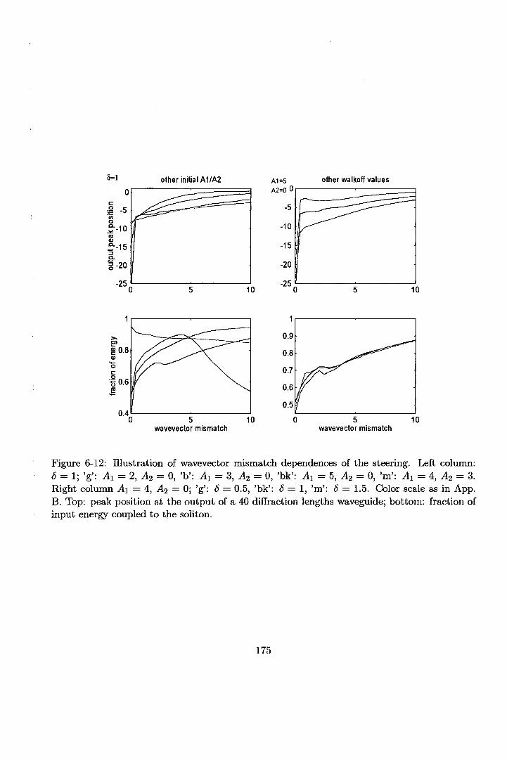
Figure 6-12: Illustration of wavevector mismatch dependences of the steering. Left column:8 = 1; 'g': A! = 2, A2 = 0, 'b': AI = 3, A2 = 0, 'bk': A1 = 5, A2 = 0, 'm': AI = 4, A2 = 3.Right column AI — 4, A% = 0; 'g': 6 — 0.5, 'bk': 6=1, 'm': 5 = 1.5. Color scale as in App.B. Top: peak position at the output of a 40 diffraction lengths waveguide; bottom: fraction ofinput energy coupled to the soliton.
175

IIIIIIIIIIIIIIIIIIIII
other initial A1/A20
-2
lo -6Q.
"S -8a.
1-10
-12
A1=5
A2=0
other wavevector mismatches
-5
-10
0.5 1 1.5 2-15
0 0.5 1 1.5 2
to.9
0.8
0.7
0.5 1 1.5walkoff parameter
0.9
0.8
0.7
0.60.5 1 1.5
walkoff parameter
Figure 6-13: Illustration of Poynting vector walkoff dependences of the steering. Left column:J3 = 3; 'g': A^ = 2, A2 = 0, 'V: AI = 3, A2 = 0, 'bk': Al = 5, A2 = 0, 'm': A1 = 4, A2 = 3.Right column Al = 5, A2 = 0; 'g': j3 = 1, 'bk': 0 = 3, 'b': (3 = 6, 'm': ft = 10. Color scaleas in App. B. Top: peak position at the output of a 40 diffraction lengths waveguide; bottom:fraction of input energy coupled to the soliton.
176

IIIIIIIIIIIIIIIIIIIII
right provided fast enough reaching of A</> ~ 0 condition by main profile takes place. Otherwise
as obtained in the AI = 5, A% = 0, /3 = 0 case (curve in black in left column of Figure 6-12), very
fast radiation to the right produced by the combined effect of on one side a sharp initial phase
distortion due to endowment of the right part of the profiles with great velocity to the right;
and on the other side, sluggish detachment from initial A<^> ~ — 7r/2, causes an extraordinary
soliton speeding up towards the left.
Figures 6-11 and 6-13 illustrate dependences upon the walk-off parameter value. Very short
velocities matching distance determines for low 6 values quick soliton formation that hinders
speeded up energy to the right be recovered by main profile specially for low (3 values. The
increase in radiation to the right enhances soliton deviation provided f3 is high enough to
guarantee fast enough detachment from A0 ~ — ?r/2 that prevents a significant part of the
generated second harmonic escaping away from fundamental (compare the results for /3 = I
and 0 = 3). For higher 6 values, the increase in the velocities matching distance which eases
the coupling of energy to the right causes the decrease in soliton deviation obtained for ¡3 = 3 .
Save for very small 6 values for which injection of a significant fraction of the energy into
second harmonic while reducing the effect of radiation prevents the soliton speeding up, again
it is shown that the position of the soliton at the output of the waveguide depends basically on
the total energy injected and only improvement of energy efficiency calls for supply of a fraction
of energy in the form of second harmonic.
6.1.2 Conclusions
This section has been devoted to analyze Power dependent steering which takes advantage of a
moderate Poynting vector walk-off, 6, present in the x^ sample. According to
the shift experienced by the soliton at the waveguide output depends basically on the energy
that through the dynamics is alloted to the second harmonic. For their practical relevance, the
study has focused in the case in which only the fundamental field is input and hence positive
wavevector mismatch values have been considered.
177

For moderate S values the transverse velocity acquired by the soliton has been seen to follow
simple rules, namely
/ t *• I\/Iî\STAT I—*• v Î (soliton detaches from propagation axis)
/3 t > h/h\STAT Î > V I (soliton approaches propagation axis)
The soliton deviation was shown to depend mainly on the amount of total power injected into
the waveguide and Very little in the fraction that initially was carried by the second harmonic.
The effect of significant fractions of input energy in the second harmonic was seen to merely
lead to some energy efficiency improvement.
With normalized values up to 6 ~ 2 entailing for typical conditions, i.e. A ~ lfj,m and
77 ~ 15/^m with T) beam width, walk-off angles of about p ^> 1 — 2°, soliton deviations around 5
beam widths with about 80% of energy efficiency have been obtained in the simulations.
As for the effect of radiation it is summarized in the following diagram:
Î » h/h\STAT Î
6 t / Η>• I\/II\STAT I
I I > h/h\STAT Î
reduced influence
v « -6I2/I
initial phase distortion speeds
radiation to the right up * v f
reduced SH phase distortion, generated
SH walks FF off —> v |
178

6.2 Angle-controlled steering
6.2.1 Numerical experiments
This section gathers up all numerical results concerning steering controlled by input light inci-
dent upon the waveguide at a certain angle with respect to the optical axis. Optical steering
control based on tilted input beams providing the system with a non vanishing total momentum
was predicted by Tomer et al [121] and some studies that consider type II geometries are found
in [124]. With interest lied in identification of effects and possibilities as well as assessment of
realistic orders of magnitude of the parameters involved, here the analysis is restricted to type
I configurations.
Although the effect of some Poynting vector walk-off will be considered at the end of this
section, configurations in which it can be neglected will constitute the main concern, having in
mind non-critical or typical QPM phase matching settings. According to (4.16) soliton steering
may then be achieved by endowing the system with a non-vanishing momentum, so that the
solitary wave that eventually emerges has transverse velocity
v K £, (6.3)
being / and J two conserved quantities, namely the total energy and momentum of the system
respectively. Transverse linear phase modulations of the input fields corresponding in practice
to simple angular tilts, i.e.
av (s,£ = Q) = UV (s) exp(-j>i/s), (6.4)
with v = 1,2, are the means by which the momentum is introduced into the system in such a
way that the transverse velocity reads
J II M2 h lc ,-,^T = -MiT-Y7- (6-5)
The fundamental beam needs to be used if solitonic wave propagation is to be obtained
through the launching of only one beam into the waveguide. In that case as a consequence of
179

IIIIIIIIII¡i
IIkiiiii¡Ii
the Galilean invariance enjoyed by the governing equations when 6 = 0, a soliton propagating
with the same transverse velocity as the input is excited resulting in a trivial steering case. Thus
interactions between tilted beams both at the fundamental and second harmonic frequencies,
using one as the signal and the other as control, will be the subject of study along the present
section.
With an eye to practical steering and routing applications, attention is focused to the case in
which the fundamental is the signal beam to steer while the second harmonic performs steering
control. Practical ways can be implemented to obtain a weak second harmonic control beam out
of the incoming fundamental signal beam or other fundamental beam accompanying it acting
as control, and readily get the required tilt to attack the waveguide. For that reason it is also
important that significant steering is achieved with low power contained in the second harmonic
control beam which advises the use of positive wavevector mismatch configurations.
According to (6.3) the soliton which eventually emerges from the interaction has approxi-
mate transverse velocity given by
/•* ^21 ,a c\v~—27^=0. (6-6)
where ¿í and I-¿ are the input values.
Figure 6-14 features a sketch of a possible practical setup. A planar waveguide structure
confines the fields along the vertical y axis whereas confinement along the x axis is achieved
through the quadratic nonlinear interaction between fundamental and second harmonic beams.
As shown, and according to the internal energy flux expressions (first terms in right hand side of
(2.113), (2.114)) and to (6.4), positive values of the linear tilt, /u, entail bright beams traveling
to the left in the drawing while negative values will indicate right direction for the beams.
Attacking the guide through different angles actually causes the extraordinary wave to
feel different refractive indexes whereupon the linear phase mismatch value slightly varies.
However for the small tilts considered in the analysis meant to keep the validity of the paraxial
approximation, this variation is assumed to be negligible although overall dependences upon
the wavevector mismatch will be investigated. Likewise, slanted incidence into the crystal may
entail appearance of a small Poynting vector walk-off whose effect is briefly outlined at the end
of the section.
Fundamental and tilted second harmonic beams which in absence of nonlinearity would
180

propagate inside the waveguide independently in different directions, mutually trap and lock
each other as a consequence of the quadratic nonlinear response of the guiding medium and
form a soliton that exits the waveguide at an intermediate position as Figure 6-15 showing the
superimposition of the evolution of the field profiles of the two harmonics in a representative
case in a linear and a nonlinear medium respectively, clearly illustrates.
The momentum initially carried out only by the second harmonic has to be communicated
to the whole system so that the solitary wave finally formed is the result of a trade-off through
which the dynamics selects among the infinite travelling wave replicas of the non walking solitary
waves existing in all directions, hopefully within the limits of the paraxial approximation, the
best suited for the initial conditions given. The process of progressive transfer and sharing of
momentum between the harmonics is illustrated in Figure 6-16 featuring the evolution of each
harmonics' energy centroid for selected cases and showing how each beam net transverse flux
of energy changes direction dynamically until the fields phase fronts and amplitude relations
and shapes are adjusted so to cancel nonlinear phase mismatch and form an oscillating state
slightly walking the z axis off. Initial tilt, total energy and amplitudes, together with the
configurations' wavevector mismatch determine the trade off value for the final propagation
angle of the emerging soliton and the fraction of the initial energy that it carries.
If radiative losses are small one could naively take (6.3) to be a good approximation of
the transverse velocity of the solitary wave finally formed and that could indeed be the case
if the radiation produced by the dynamics of soliton formation was symmetric and thus the
momentum stolen from the soliton had zero average. The fact that asymmetric radiation will
be produced is clear from the viewpoint that the initial phase front profile imposed by the tilt
creates differentiate zones with opposite signs of the initial energy exchange between harmonics
(see Figure 6-26) which therefore undergo different dynamics.
An arrow in Figure 6-15 indicates the position at the waveguide output that would approx-
imately correspond to the energy centroid had it travelled at the transversal velocity dictated
by (6.6). The difference obtained is mainly due to the momentum carried by radiation which
does not have zero average as reflected also by the plot in Figure 6-15, as a consequence of the
asymmetry in the energy exchange between harmonics introduced by the tilt.
Once the main features of the phenomenon of beam trapping creating solitons walking in
181
15
S 10
o"to01taa.o
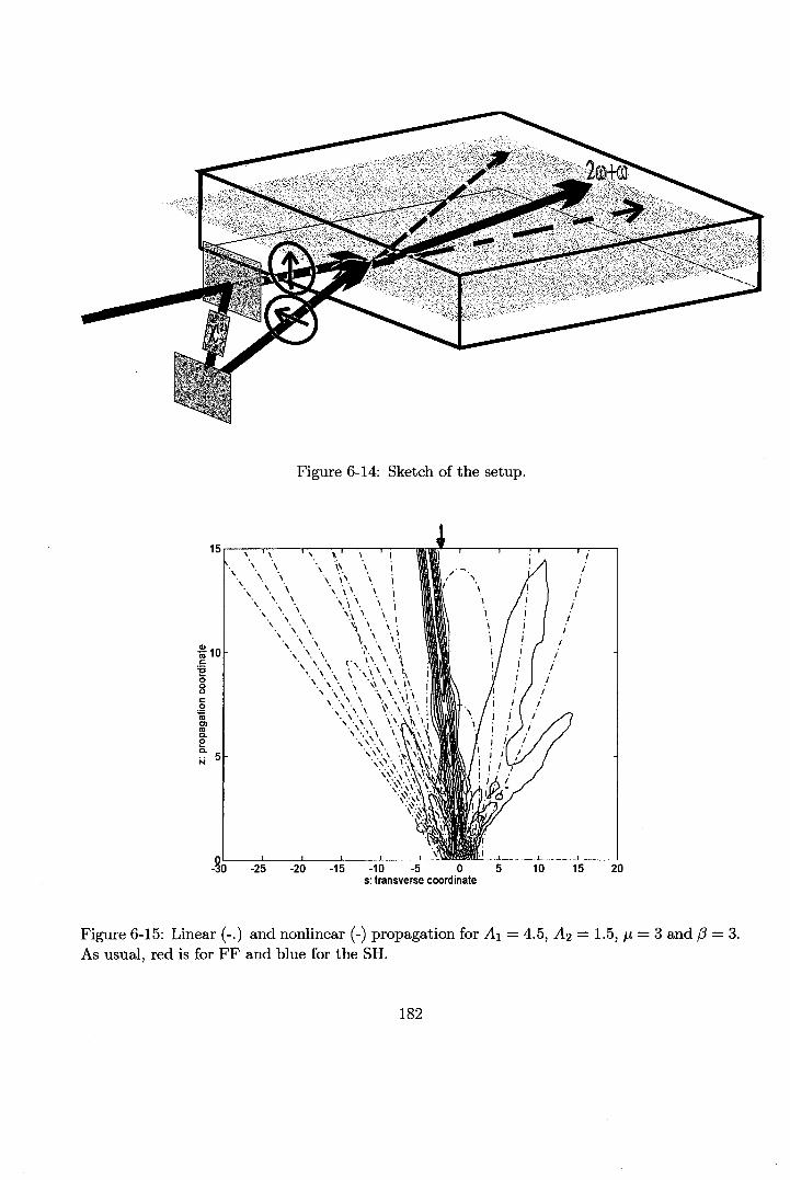
Figure 6-14: Sketch of the setup.
\ \ \ \\\ \ i\ N \ ^ '\ ' !
\ \\ \ X \\\\\,. v\ \
30 -25 -20 -15 -10 -5 O 5 10 15 20s: transverse coordinate
Figure 6-15: Linear (-.) and nonlinear (-) propagation for AI = 4.5, A% = 1.5, ¿t = 3 and /3 = 3.As usual, red is for FF and blue for the SH.
182

a)0.2
g ~°-2
o -0.6
1-0.8
10
b)
O
-0.5
-1
-1.5
-2
-2.5
-3O 10
d)
O
-0.5
-1
-1.5
-2
-2.5
10z: propagation variable z: propagation variable
Figure 6-16: Evolution of energy centroids in some typical cases. As usual red is for thefundamental and blue is for the second harmonic, (a): /? — 3, AI = 4.5, AI = 1.5, fj, = 1; (b):same but fj, = 3; (c): same as a) but AI = A% = 3; (d): same as c) but /3 = —3.
183

IIIIIIIIIIIIIIIIIIIII
different directions through injection of tilted beams which introduce a certain momentum into
the system have been outlined, the implications for efficient steering control are considered.
To begin with, the feasibility of input angle control of the steering is analyzed. The prop-
agation of the fields along a waveguide 40 diffraction lengths long has been simulated using a
split-step Fourier method.
A tilt value of fj, < 4, corresponding for typical conditions, A ~ l/¿m, r\ ~ 15/j.m, to an input
angle of about
0 = arctan ( -^-] = 1.3°, (6.7)-
is taken as a safety limit to guarantee the applicability of the paraxial approximation.
The profiles considered have a Sech like transversal dependence so that the inputs provided
to the numerical algorithm have the form
,(6.8)
a2(£ = 0, s) = A-¿Sech(s) exp(-j/j,s),
Some examples of angle steering control are shown in Figure 6-17.
The position in beam widths units of the soliton which eventually emerges at the output as
well as the fraction of the incident energy that has been coupled to it are plotted in Figure 6-18.
The curves reveal that efficient beam steering on the order of 5 beam widths with reasonable
energy efficiencies on the range of 80% can be achieved. Other initial amplitudes and other
wavevector mismatches yielded analogous results thus confirming the robustness of the steering
method and rendering the configuration perfectly suited for the design of practical applications.
A remarkable feature pointed out by the plots in Figure 6-18 is the existence of an optimum
value of the initial tilt that maximizes beam deviation. Above this optimum value the transver-
sal velocity induced by the tilt onto the second harmonic is so high that the fundamental is not
able to trap it and much of the second harmonic energy escapes carrying a significant part of
the total momentum it has introduced into the system. Below this optimum value, influence of
the tilt on the initial energy exchange between harmonics produces a small amount of radiation
that travels in the direction opposite to the one imposed by the tilt thus enhancing the steering.
This effect is more evident for small wavevector mismatch setups since the initial amplitudes
184

ANGLE CONTROL
ID•O
I2n(O
11
-10 -8 - 2 0 2s: transverse coordínate
10
Figure 6-17: Input and outputs at 40 diffraction lengths demonstrating angle control of thesteering. In all cases 0 = 3. (-) FF amplitude profile, (- -) SH amplitude profile.
other A1/A2 other wav. mismatches
i -2
1-4Q.
-* Cre -o<Do.3 -8CL
0-10
-123 4
2 3initial tilt
1 2 3initial tilt
Figure 6-18: Features of angle controled steering. Left: different input amplitudes with (3 = 3.('m' lines) AI = 4, (- -): A2 = 0.5, (-): A2 = 1, (-.): A2 = 2, (:): A2 = 3. ('g' unes) AI = 6,(-): AI = 0.5, (- -): A2 = !,(-.): A2 = 1.5, (:): A2 = 2 . Right: different (3 values with AI = 4,A2 = 1. ('m' Une): 0 = 3, ('b'-): 0 = 0, ('b'- -): 0 = 6, ('b'-.): 0 = 10. Color scale as in App.B.
185

IIIIIIIIIIIIIIIIIIIII
fall further away from the values needed for the stationary solution and the dynamics of beam
trapping requires a longer propagation length.
Next series of numerical experiments aimed at demonstrating the possibility of control-
ling the deviation of the trapped beam through control of the energy contained in the second
harmonic control beam yielded the results shown in Figures 6-19, 6-20 and 6-21.
These results evidence great sensibility of the steering on the initial power content in the
second harmonic due both to influence on the momentum introduced into the system according
to J = — /¿/2/2 and also due to its effect on the dynamics towards the reach of a stationary
state.
Specifically, Figure 6-21 shows in its top row plots whose curves all feature the same value of
expected velocity according to (6.6), that when the total energy flow, /, is increased, due to the
reduction in nonlinear interaction length easing momentum sharing between the harmonics,
faster solitons are obtained. The increase in soliton velocity is less evident for small second
harmonic energy fractions of the total energy due to the decrease in the stationary energy flow
relation, Ii/l2\STAT, which takes place with an increase of / and that tends to enlarge the
nonlinear interaction length. A similar argument considering the influence of the wavevector
mismatch, /?, on the nonlinear interaction length explains the curves obtained in 6-21 bottom
row. In this sense it is observed for very low total input powers and high wavevector mismatches
in Figure 6-21 that the difficulties that an input second harmonic power increase poses as for the
reaching of a stationary solution that features a very low second harmonic power content lead
to obtention of very small soliton deviations and of course poor energy efficiencies in spite of the
total momentum into the system being increased. Finally, also thinking on the feasibility to
perform temperature control of the steering, the dependences upon the wavevector mismatch
present in the system were evaluated. The results in Figures 6-22 demonstrate the robustness of
the steering effect although the deviation of the peak obtained as well as the energy coupled to
it strongly depend on the wavevector mismatch value. Mind that, opposite to initial tilt value
and initial power or power fraction which determine different values for the expected velocity as
given by (6.6), the wavevector mismatch dependence of soliton steering steams uniquely from
its influence upon the parametric interaction through which the initial momentum is introduced
into the system. In short, the conclusion extracted from these plots is that as the wavevector
186

POWER CONTROL
-10 - 5 0 5s: transverse coordinate
10 15
Figure 6-19: Inputs and outputs at 40 diffraction lengths demonstrating power control of thesteering. In all cases f3 = 3, /j, = 3.
OTHER TILT VALU ES OTHER WAVEVECTOR MISMATCHES
-2
g. -4r̂a8. -6•3Q.
2 -8
-10
-2
-4
-6
-8
-10
1><eng 0.90)
1-0.8
"o
.i07
Î5^ 0.6
O 1 2initial SH amplitude
1
0.9
0.8
0.7
0.6
1 2 3initial SH amplitude
Figure 6-20: Features of power controlled steering for other values of the initial tilt and otherwavevector mismatches, 'm' lines: AI = 4, AI = 1; 'g' lines: A\ = 6, AI — \ . Left: (- -) f¿ — 1;(-.) M = 2; (-) M - 3; (:) M = 4. Right: ('b-') /? = 1; ('m') 0 = 3; ('b- -') 0 = 6; ('b-.') 0 = 10.Color scale as in App. B.
187

IIIIIIIIIIIIIIIIIIIII
output peak position
0.1 0.2 0.3 0.4 0.5 0.6
0.1 0.2 0.3 0.4 0.5 0.6
l=36
0.1 0.2 0.3 0.4 0.5 0.6% of initial energy into SH
1
0.9
0.8
0.7
0.6
0.51—••
fraction of energy
0.1 0.2 0.3 0.4 0.5 0.6
1
0.9
0.8
0.7
0.6
0.5"—-0.1 0.2 0.3 0.4 0.5 0.6
0.1 0.2 0.3 0.4 0.5 0.6% of initial energy into SH
Figure 6-21: Features of power controlled steering. /3 = 3, I = 36, /¿ = 3 unless stated otherwise.Top (V): 7 = 8; ('g'): / = 18; ('bk'): / - 36; ('m'): / = 50. Middle ('m'): ¡í = 1; ('c'): M = 2;('bk'): M = 3; ('g'): fi = 4. Bottom ('m'): P = 0; ('g'): /? = 1; ('bk'): 0 = 3; ('r'): 0 = 6; ('b'):f3 — 10. Color scale as in App. B.
188

IIIIIIIIIIiIIIIIIIIII
obtained at the expense of a poorer energy efficiency due to the influence of radiation whose
direction opposes that of the tilt.
For getting a feeling on how radiation impacts upon the transverse velocity of the soliton
finally formed and recalling that for a given total power, proximity to the stationary solution
depends basically on the harmonics amplitude relation in such a way that to a great extent it
determines the amount of radiation to be expected, in the next set of numerical experiments
inputs with the same total power I but different amplitude relation between harmonics A\/A-¿
are considered (Fig 6-23).
In all cases an optimum value of ¡JL for which the steering is maximum is obtained which
is smaller and gives better deviation than predicted by (4.16) for big A\/A¿ while slightly
greater and giving worst steering than predicted for small Ai/Az (see the curves in bottom
row). The existence of this point of maximum soliton deviation and its dependence upon the
initial amplitude values is understood by considering that for efficient nonlinear coupling of
first and second harmonic which enables the momentum carried by the second harmonic to be
shared with the fundamental, the second harmonic left shifting tendency needs to be initially
slowed down under the influence of the fundamental amplitude. The faster and more powerful
the second harmonic the more powerful has to be the fundamental to realize the trapping
and consequently this maximum steering initial tilt value is smaller as the relation A\/Az is
decreased.
A too fast and powerful relative to the fundamental second harmonic beam is shown to be
detrimental for the steering because as not efficiently slowed down by nonlinear interaction with
the fundamental, a great part of its energy walks the main fundamental beam off so that only
a small fraction of fundamental wave is able to follow it. The fast traveling second harmonic
along with the portion of fundamental that it has somehow managed to pull up from the main
profile selfishly retain a significant part of the momentum injected into the system and may
form a soliton above a threshold power as shown in Figure 6-24 bottom row, but in any case
abandon the main part of injected fundamental beam so that solitons carrying a significant
part of the injected energy are necessarily slow.
The fact that the second harmonic literally abandons the fundamental is evident in Figure
6-25 bottom row where the amplitudes evolution in symmetric waveguide longitudinal cuts
189

IIIIIIIIIIIIIIIIIIIII
6-25 bottom row where the amplitudes evolution in symmetric waveguide longitudinal cuts
located far away from the area where soliton propagation takes place, yields analogous behavior
of radiation in the case of a too fast second harmonic beam and that of no injection of any
second harmonic with the difference of some fast radiation to the left observed in the second
harmonic amplitudes plot indicating the injected second harmonic is leaving the scene.
It is important to note that since the total momentum in the system has to be conserved
the initial second harmonic slowing down effect needs to be payed for so that it takes place in
a reduced central part of the profile while outer parts actually result speeded up, see Figure
6-26. If the velocity imprinted to these outer parts is small compared with that of the nonlinear
interaction, a great deal of their energy can eventually be recovered by the main profile.
On the other hand, the initial transverse linear phase front variation imposed on the second
harmonic input beam yields differentiate areas at each side of the s = 0 point with opposite
signs of the inter harmonics energy flow and therefore it severely influences the dynamics in
such a way that for the input conditions considered here, soliton formation is eased for s < 0
whereas it is hindered for s > 0, Figure 6-26.
The effect is more pronounced for big A\jA-i values and that is seen in Fig 6-23 in the
increase of energy coupled to the output soliton for small values of /x as the relation Ai/Az
is decreased. The added loss observed for big values of fj, as the AI/'AI relation decreases
corresponds to radiation to the left produced by a strong second harmonic pushing hard to the
left and a weak fundamental not capable of trapping it.
The plots in Figure 6-25 constitute a good illustration of the influence of the initial tilt on
the asymmetry displayed by radiation. In Figure 6-24 it is shown how when the total power
is increased the small fraction pulled up by the second harmonic from main profile is able to
form a soliton for large initial left traveling speeds, whereas when this initial velocity is small a
soliton traveling to the right is formed by the residual radiation produced at the right part of
the profiles because of the asymmetry in energy exchange.
Figure 6-23 bottom row, shows the soliton peak position shift with respect to the one
expected if the momentum carried by radiation had zero average. As a consequence of radiation
being minimized, the steering observed is almost equal to the expected until a too big value of
the initial tilt makes it impossible for the fundamental beam to slow the second harmonic down
190

IIIIIIIIIIIIIIIIIIIII
Likewise, when taking equal values of the relation AI/AZ but different total input powers as
in Fig 6-23 right column, which is equivalent to consider equal values for the nominal velocity
as given in 4.16, it is observed that the value of \i for which the steering is maximum decreases
as the total power is increased and that is explained by the fact that for higher total power the
amplitudes stationary values are further away from the initial Ai/A% relation considered in this
case which as entailing a longer time required to realize the trapping, ease second harmonic
walking the fundamental beam off. The plot for the fraction of energy into the soliton in Figure
6-23 right column, bottom row, shows agreement giving less energy coupled for higher input
powers.
Enhanced coupling of energy initially located at the s > 0 side of the profiles into the soliton
takes place when a value of ¡JL is reached which causes the appearing in a transversal coordinate
to the right side of the profiles with relevant field amplitudes, of an additional area to be initially
affected by an energy flow from fundamental to second harmonic which fast enough is capable
of getting close to A0 = 0 condition. On the other hand for the same initial tilt value, an
increase of radiation to the left is produced as a consequence of swift escaping to the left of
an area of second harmonic to fundamental energy exchange at the s > 0 part of the profiles
not efficiently influenced by the initial phase distortion. The combination of both effects causes
the decrease in soliton deviation with energy efficiency maintenance observed in the curves for
large /¿ values.
In other words, it is the existence of two zones with opposite sign of the energy flow at each
side of s = 0 for a large value of fj, as illustrated in Figure 6-26 which gives fast left travelling
and hence stealing part of the initial momentum radiation for s < 0 and big left travelling fluxe
and hence coupling more of the energy initially located at the right part of the profiles into the
soliton for s > 0 causing the soliton to slow its left shift down while keeping the fraction of
input energy it carries for large values of (¿.
At this point it is useful to analyze in detail the process of beam trapping. Figure 6-
26 illustrates how under the influence of the strong fundamental beam through the nonlinear
response of the medium, the second harmonic undergoes a phase front smoothing that slows
its left shift tendency down. Also the asymmetric energy exchange (gain for s < 0, loss for
s > 0) becomes apparent. These two features are captured by analytically solving the governing
191

I1
s > 0) becomes apparent. These two features are captured by analytically solving the governing
I equations under the assumption of no significant variation of the fundamental frequency beam.
One readily finds
o-ï (£1
, s) = o2 (0, s) exp (-J0Ç) + —ma\ (0, s)2 * exp (-2A//3|s|) (1 - exp (-J0Ç)) .\ /
(6.9)
For the specific input field profiles analyzed here, and phase mismatch values on the range of
1 (3 ~ 3 — 10, by writing the fields in the form a — U exp(j</>) the above may be approximated by
1. Fig 6-27
TT?o2 (£, s) ~ U2 exp (-j (fis + /?£)) + ̂ - (1 - exp (-J0Ç)) . (6. 10)
demonstrates the accuracy of this approximation in modelling the evolution of the
• second harmonic beam for small propagated distances.
15
1"
Í4oQ-
|
O> 0
iQ.
E2
1 :ïi
°
WAVEVECTOR MISMATCH CONTROL AND TOLERANCES1 ' expected
O f f
P=6
fk"3 / \
A ° / V // / \ \ / y /i \ I - A /
- / V' m_Ji¿uJí-,,rr^T— fL -u =e^ ̂ =
-10 -5
>osition' ' 'eak
/ \/ \/ \
\/ \ \
(\ \ \
0 5 10s: transverse coordinate
1Figure 6-22: Input and outputs of a 40 diffraction lengths waveguide illustrating wavevector
1mismatch dependences of the steering. AI — 4, A-¿ — 1, u, — 3.
1
1
1
1
1
1
192

i
l=36 A1=1.5A2o
-2
-4
'"§ -6oQ.
* -8ta "<a
-12
-14
a)-1
-2
-3
-4
-5
-6
-7
d)
0.95
0.9
0.85
0.8
0.75
0.7
0.65
e)
o
-5
-10
-15O
c)
2initial tilt
5
4
3
2
1
0
-1
-21 2 3 4
initial tilt
Figure 6-23: Features of the steering for ft = 3. Left: ('g' Unes): AI > A^ ('m' lines): A\ < A%.('g'-): Ai = 4.12, A2 = 1; ('g'- -): AI = 4, A2 = 1.4; ('g'-.): AI = 3.85, ¿2 = 1.8; ('g':):¿i = 3.5, Ai = 2.4; ('m'-): AI = A2 = 3; ('m'- -): AI = 2.7, A2 = 3.25; ('m'-.): AI = 2.4,A2 = 3.5; ('m':): AI =2,A2 = 3.25. Right: ('b'-): / = 19.12; ('b'- -): / = 34; ('b'-.): / = 53.12;('b':): / = 76.5. Color scale as in App.B.
193

- 5 0 5s: transverse coordinate
10 15
<D
¡ 10
O) O•o
i 6ci-
ca 4CO
-15 - 5 0 5s: transverse coordinate
10 15
Figure 6-24: An additional low energetic soliton is formed travelling to the right for fj, = 2 andto the left for ¡j, — 3.5. In both cases A\ = 10, AI = I , /3 = 3 and the outputs are taken at 40diffraction lengths.
194

FF SH0.25
0.2
0.15
0.1
0.05
0
0.2
0.15
0.1
0.05
10 15 20 10 15 20
0.25
0.2
0.15
0.1
0.05
0.25
0.2
0.15
0.1
0.05
0 10 15 20 10 15 20
0.5
0.4
0.3
0.2
0.1
5 10 15z: propagation variable
20
0.3
0.25
0.2
0.15
0.1
0.05
0 5 10 15z: propagation variable
20
Figure 6-25: Amplitudes évolution in longitudinal waveguide cuts in symmetric transversepoints s = —30 ('g'), s = 30 ('m') to illustrate the behavior of radiation. AI — 4, AI = 1,(3 = 3, and /x = 0.5 (top), \i = 2 (middle) and fj, = 4 (bottom). In top an middle row the 'm'line corresponds to the same amplitude evolution in the no tilted case and in bottom row, itshows the case AI = 4, A-¿ = 0. Color scale as in App. B.
195

it units
-2.5 -2 -1.5 -1 -0.5 O 0.5 1s: transverse coordinate
1.5 2
-2.5 -2 -1.5 -1 -0.5 0 0.5s: transverse coordinate
1 1.5 2 2.5
Figure 6-26: Second harmonic amplitude and phase profiles in the first steps of propagation forAI = 4, AÏ = 1, p = 3. 'bk': input; ('m'-): ¿ = 0.05; ('m'-.): £ = 0.1. Top: fj. = 2. Bottom:fj, = 3. Color scale as in App. B.
196

2.5
0.5
oQ_
COO)10asj=O.T3
ro „<D O
as
- 3 - 2 - 1 0 1s: transverse coordinate
Figure 6-27: SH amplitude and phase profiles for £ = 0.05 for the same case as previous figure,top row, as obtained from the numerical bpm ('b'), and using the approximation of undepletedfundamental ('m').
197

IIIIIIIIIIIIIIIIIIIII
Soliton steering for other values of the wavevector mismatch is illustrated by the plots in
Fig 6-28. The previous analysis explains worst steering but more energy coupled to the soliton
for ft = 10 because being the initial amplitudes closer to the values for the stationary solution
in this case, the influence of radiation is minimized.
As usual it will be the requirements of any given practical application to decide whether one
needs to save energy and hence would rather choose a large mismatch value or should worry
further about achieving a significant soliton deviation whereupon a lower ft value should be
pursued.
To complete the analysis of the wavevector mismatch dependence, the case of zero wavevec-
tor mismatch configurations is also analyzed using the plots in Figure 6-29.
As expected, the slowness of the nonlinear interaction causes a lot of radiation of both signs
resulting in an almost constant steering with also almost constant energy coupled to the soliton
for initial tilt values above //, ~ 2.5 very becoming for practical applications because no precise
control of the input angle is required, allowing even its use as an angle stabilizator. The sudden
drop in soliton energy accompanied by significant enhancement of the steering observed in the
plots was confirmed to steam from formation of another less energetic soliton travelling to the
right.
The case of tilted fundamental beams was also investigated setting (3 = 3 yielding the results
in Figure 6-30.
Being the initial energy exchange imposed by the tilt second harmonic to fundamental at
the s < 0 part of the profiles, soliton deviation is expected to result reduced for Ai/Az >
AI/AZ\STAT while enhanced for Ai/A-¿ < A\¡A<¿ STAT, just as the plots show. It is worth
emphasizing the fact that because the momentum acquired by asymmetric radiation produced
for lower Ai/A% relations introducing lower total momentum into the system and therefore
expected to yield slower solitons, enhances the momentum finally coupled to the soliton formed,
an almost constant output soliton position is obtained almost regardless the initial A\/Az
considered.
Next the case of negative phase mismatch configurations is briefly examined.
First, attention is focused to the case in which the tilt is applied to the weaker beam which
for the sake of energy efficiency needs to be the fundamental. The results in Figure 6-31 quite
198

peak
shi
ft
W U
T. ^1
V
*> O
**?•
í-l
**>
~-M
?B ̂ ,-
to
œ
O
00
O
) -U
N
JO
M
fract
ion
of e
nerg
yp
p
p
p
pbi
ò)
^
bo
¿o
I I
peak
pos
ition
ço
to
->•
O
-»
M
CO
CO
«O
Bhi
S^
^s-
- t-1
s^S
»I
II _
C5 ^ k II v
/*l*
\ "
p .31
op
p
oo
P
ço00
01
ÇO
01
CO
J
M
> II
E «-^

II
p=oo
(Ooo.
-15
1=36
-5
-10
-15
A1=1.5A2
0.9>,O)a>S 0.8"o
J 0.7"oE
0.6
0.5
1
0.9
0.8
0.7
0.6
0.5
0.4
(Od>CL
-2
2 3initial tilt
15
10
1 2 3 4initial tilt
Figure 6-29: Features of the steering for /? = 0. Left: ('g'-): AI = 4.12, A2 - 1; ('g'- -): AI = 4,A2 = 1.4; ('g'-.): Aj. = 3.85, A2 = 1.8; ('g':): AI = 3.5, A2 = 2.4; ('m'-): AI = A2 = 3. Right:same as in Figure 6-23. Color scale as in App. B.
200
l=36 A1=1.5A2
-10g
ü)oQ.-
<O0>Q.
-30
-400.5 1 1.5
-10
-20
-30
-400.5 1 1.5
0.95
0.9
0.85
0.8
0.75
0.7
0.650.5 1 1.5
15
10
.mO)o.
-5O 0.5 1 1.5 2
initial FF tilt
-1
-2
-3
-4
-5O 0.5 1 1.5 2
initial FF tilt
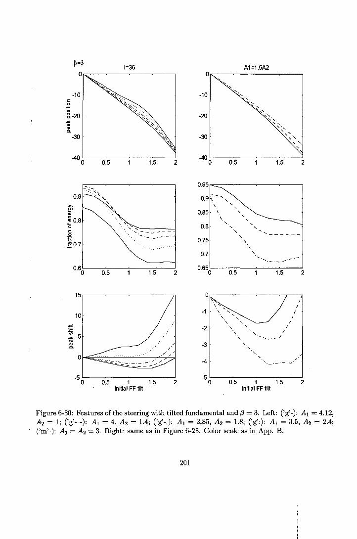
Figure 6-30: Features of the steering with tilted fundamental and /? = 3. Left: ('g'-): A\ = 4.12,A2 = 1; ('g'- -): Al = 4, A2 = 1.4; Çg'-.): Al = 3.85, A2 = 1.8; ('g':): ^ = 3.5, A2 = 2.4;('m'-): AI = AZ — 3. Right: same as in Figure 6-23. Color scale as in App. B.
201

1=36 A2=1.5A1
-2
-4
-6
-8
-100.5 1 1.5
0.9
2>0>c0>
"o
0.8
o 0.7ôS
0.50.5 1.5
J*ma>o.
-5
-100.5 1 1.5 2
initial FF tilt
10
8
6
4
2
0.5 1 1.5 2initial FF tilt
Figure 6-31: Features of the steering with /? = —3, and tilted fundamental. Left: ('g'-): AI = 1,A2 = 4.12; ('g'- -): Al = 1.4, A2 = 4; ('g'-.): Al = 1.8, A2 = 3.85; ('g':): Al = 2.4, A2 = 3.5.Right: same as in Figure 6-23. Color scale as in App. B.
202

closely resemble those in Figure 6-23 featuring as well an optimum initial tilt value in terms of
soliton deviation obtained which decreases as the momentum injected into the system increases
as a result of easier weak beam escaping from the interaction with the non-tilted strong beam.
Also better soliton velocity enhancement is achieved through the action of asymmetric radiation
when the initial amplitude relation falls further away from the stationary value, that is, the
AI/A% amplitude relation increases.
When the tilt is imposed upon the second harmonic the dynamics of soliton formation in the
less versatile negative wavevector mismatch case results severely obstructed by the asymmetric
energy exchange pattern, so that for high values of the tilt only the use of initial amplitude
relations very close to the stationary values allows for neat soliton formation.
The dramatic influence of the sign of the phase front on the final position of the soliton
makes interesting the following study of the effect of an initial constant phase mismatch between
harmonics <p0. That influence is manifested even when no initial transverse phase variations are
imposed into neither of the harmonics, i.e. the system possesses zero momentum, by splitting
the beams in the case $0 = IT (Figure 6-32). Such an splitting is due to the change in sign of
the phase front distortion undergone by the two harmonics in the initial steps of propagation
which leads to opposite travelling energy fluxes at each side of the s = 0 point.
The numerical results obtained for different values of the initial relative phase imposed be-
tween harmonics, </>0, in Figure 6-33 evidence a change in the soliton shift dependence with
respect to the initial tilt which basically consists in an improvement of output position discrim-
inance for 4>0 < 0 and a tendency to reduce it even leading to solitons deviation towards the
opposite side as that pointed by the initial tilt for cj)0 > 0.
Qualitative understanding comes from evaluation of the effect of the initial phase difference
in both the transverse energy exchange zones and in the initial phase front distortion undergone
by the initially tilted beam.
For a negative (f>0 value this effect is on one side to bring the zone of initial detrimental
energy exchange (second harmonic to fundamental) from the right hand side to the center of
the field profiles causing an increase of the energy that results radiated to the right, and in
the other side, that the transversal coordinate at the s > 0 side of the profiles where the
function Sech(s) cos(/j,s — 00) that approximates the transversal dependence of the phase front
203

. . " " • ' ' • • • " ' •'-'"'.>v*^%^fà$Í$i^.. , :-;4 ;.-'••• •;• ".'•• .':/v,^-.-'f;/-;*;*
-8 -6 -4 - 2 0 2s: transverse coordinate
8 10
Figure 6-32: Example of splitting due to initial phase differences between the harmonics. Here(/>0 = 7T, 13 = 3, A! = 4, A-2. = 1.
204

i -2
os -4<D
-8
6
4
2
O
-2
0.95
2initial tilt
2initial tilt
Figure 6-33: Influence of an initial phase difference between harmonics. In all cases AI = 4,Ay = 1, ¡3 = 3. ('bk'-) shows the 00 = 0 case, (bk-.) is the expected position regardless theeffect of radiation. Left: ('g'-): -Tr/10, ('g'- -): -Tr/5, ('g'-.): -w/4, ('g':): -T/3» (b-): ~7r/2-Right: ('m'-): ?r/10, ('m'- -): 7r/5, ('m'-.): 7r/4, ('m':): Tr/3, (b-): 7T/2. Color scale as in App.B.
205

IIIIIIII
distortion undergone by the second harmonic is minimum, falls closer to the center so that the
second harmonic transversal phase front gets considerably sharpened at this point conferring big
velocity to the right to the radiation. Greater phase front sharpening and therefore faster right
radiation leading to better steering is expected as </>„ is made more negative and the minimum
of the function Sech(s) cos(/xs — <p0] approaches the center.
As the plots in Figure 6-33 show, the value of /L¿ for maximum steering, that is to say,
the value of ̂ for which the inclusion of an additional zone of fundamental to second harmonic
energy exchange at the s > 0 part of the profiles eases the coupling of energy otherwise radiated
to the right, must be lower as the initial (j)0 gets more negative since the values of <j)0 and ¡j, for
relevant left travelling fiuxe coming from the right part of the profiles have to verify
(j)0 - p,drfa < -7T, (6.11)
where drfa gives the distance from the center of the profiles for a point at the s > 0 area to be
affected by relevant field amplitudes. That is actually the tendency shown in Figure 6-33.
Following this line of reasoning, when positive initial phase differences between harmonics
are considered, the area of energy exchange from second harmonic to fundamental is pushed
away from the center of the profiles so that less energy can escape to the right with ensuing
steering reduction. As about the phase distortion that results from the nonlinear interaction
between the two harmonics and whose transversal dependence is mainly given by the function
Sech(s) cos(fj,s — (j)0), the addition of a positive 4>0 moves its minimum at the s < 0 side
of the profiles so that it progressively gets closer to the center thus leading to more energy
radiated to the left while coupling more energy to the right coming from the maximum of
Sech(s) cos(/j,s — (/>„) getting further away from the center to the s > 0 part of the profiles.
That is the situation for low values of /j, leading to impairment of the steering with respect to
the case of harmonics in phase and even soliton deviated to the right.
Bigger values of /¿, starting from approximately ¡j, = 0.6, cause radiation to the right to
slightly increase as the maximum of Sech(s) coséis — <^>0) returns slowly to the center of the
profiles resulting in smoothing of the curve giving greater deviation to the right for the soliton
as fj, increases. Naturally this swinging of the maximum of the transverse phase front profile
206

also occurs but in a symmetrical way for <j)0 < 0, but its effects there are not that evident since
it follows the natural tendency of the steering.
A change in tendency, i.e. greater deviation to the left as fj, increases is then observed
coming from an increase in the velocity of radiation to the right as the minimum of the function
Sech(s) cos(/j,s — 00) at the s > 0 part reaches a significant field amplitudes area and progresses
towards the center of the profiles. Further increases of // cause the point for </>2 = — TT to fall in
an area of relevant field amplitudes and couple some of the energy at the s > 0 part so that it
is no longer radiated. The transverse left travelling soliton results thus slowed down and the
tendency of the steering changes again to give soliton more deviated to the right as fj, increases
starting around ¡À, ~ 3. The following relationship
(j)0 - fjdrfa < -7T
approximately holds for the values of 00 and /¿ for which significant coupling of energy at the
right part of the profiles takes place.
To complete the analysis of steering control through input tilted beams the effect of a certain
Poynting vector walk-off is briefly investigated.
The differentiate nature of Poynting vector walk-off and initial tilts as mechanisms to pro-
duce soliton deviation is illustrated in the plots in Figure 6-36. While the former as determining
a more probable direction inside the material whereupon it acts directly upon the governing
equations, gives rise to a clear and robust steering tendency, the latter as relying only upon
initial conditions is susceptible of being strongly modified through the dynamics and hence is
more fragile.
Since the energy introduced into the system is continuously pulled out in the direction
in which the walk-off points, the effect of initial tilts is through the dynamics progressively
minimized so that the range of soliton output positions obtained by changing the initial tilt
gets reduced and hence so gets the performance of an steering device based on angle control.
However as seen, if the walk-off is kept within moderate values on the range 0 ~ 1 and the
device is operated so that the tilted input beam points in the same direction of the walk-off, a
good output position discrimination is obtained.
207
IIIIIIIII -20
-20
different walkoff parameter values
-15 -10 -5 0 5 10
different wavevector mismatch values
15 20
-15 -10 - 5 0 5s: transverse coordinate
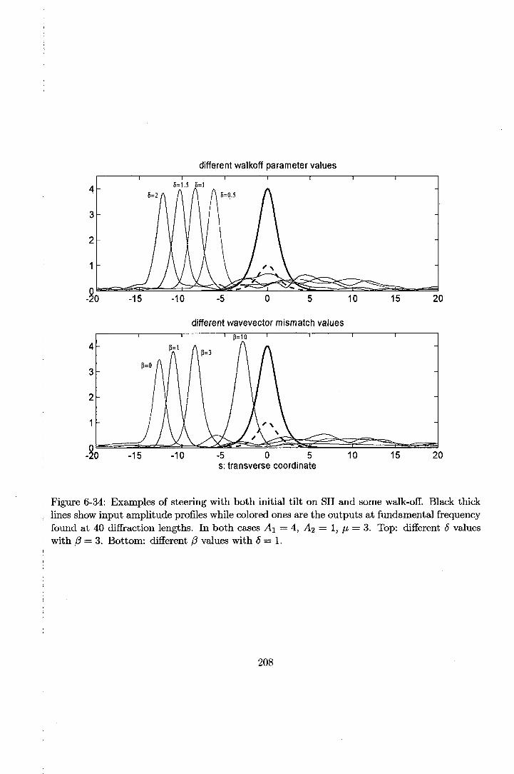
Figure 6-34: Examples of steering with both initial tilt on SH and some walk-off. Black thicklines show input amplitude profiles while colored ones are the outputs at fundamental frequencyfound at 40 diffraction lengths. In both cases AI — 4, A% = I , fj, = 3. Top: different 6 valueswith /5 = 3. Bottom: different (3 values with 6=1.
208

-20
different tilt values
-10 - 5 0 5
different SH amplitudes
-15 -10 - 5 0 5s: transverse coordinate
10
10
15
15
20
Figure 6-35: Same as previous figure showing power and angle control of the steering. In bothcases AI = 4, /3 = 3 . Top: A2 = 1; (-): 6 = !,(-.): 6 = -1; 'bk': 'b> = O, p = 1, 'g': p = 2,'r': fi = 3, 'c': \í = 4. Input profiles shown in black thick lines with (-) for FF and (- -) for SH.Bottom: fj, — 3, 6 = 1 and input second harmonic as shown by the corresponding black andcolored line. Color scale as shown in App. B.
209

15
10
5
oin2.ca
-10-15
0Q. -
CO<DCL
-10
-150.5 1.5
|o.9c<D
"o
otíS
0.8
0.7
1 2 3 4initial tilt
0.5 1 1.5walkoff parameter
Figure 6-36: Effect of some walk-off on input tilts steering. In all cases AI = 4, A% = 1, @ = 3.Left fj, = 3 ; ('g'-): 6 = -0.5, ('g'- -): S = -1, ('g'-.): 6 = -1.5, ('g':): S = -2, ('m'-): S = 0.5,('m'- -): 6=1, ('m'-.): 5 = 1.5, ('m':): 6 = 2. Right 6 = 1; ('g'-): M = 1, ('g'- -): M = 2, ('g'-.):¿i = 3, ('g':): fj, = 4, ('m'-): ¿¿ = -1, ('m'- -): /j, = -2, ('m'-.): p, = -3, ('m':): fj, = -4. Colorscale as in App. B.
210

IIIIIIIIIIIIIIIIIIIII
As increasing the transverse velocity initially acquired by the second harmonic, positive 6
values ease its escaping away from fundamental resulting in the decrease in energy efficiency
and the drop of the maximum steering initial tilt value observed in the plots. On the other
side negative 6 values as initially slowing down the transverse velocity induced into the second
harmonic cause an increase in the maximum steering initial tilt value.
As regarding power control of the steering the soliton output position stabilization effect
produced in the presence of walk-off shows interesting implications. It is observed that when
the input tilt points in the direction opposite to that determined by the walk-off, the soliton
output position basically depends only on the fraction of energy contained into the second
harmonic and not on the total energy introduced into the system and it is so in a significant
range of wavevector mismatches and with energy efficiencies within reasonable levels. This is
good news as for the building up of real devices since one needs not worry about the total power
introduced into the system but only about the fraction of this power corresponding to second
harmonic which significantly eases the practical setup required.
211

output peak position fraction of energy
1 0.2 0.3 0.4 0.5 .1 0.2 0.3 0.4 0.5
B=3 -5
-10
-15.0.1 0.2 0.3 0.4 0.5
fraction of input energy into SH
0.8
0.6
0.4
0.1 0.2 0.3 0.4 0.5fraction of input energy into SH
Figure 6-37: Effect of some walkoff on power controlled steering for /3 = 1 (top) and /? = 3(bottom) and different power values. In all cases fj, = 3. 6 = — 1 (g-): 1 = 8, (g- -): / = 18,(g_.): I = 36, (g:): I = 50. 6 = 1 (m-): 1 = 8, (m- -): / - 18, (m-.): I = 36, (m): I = 50.Color scale as in App. B.
212

TIIIIIIIIIIItIII
IIII
6.2.2 Conclusions
Soliton steering through input weak tilted beams has been analyzed in this section. Although
the main effects have been shown to occur also in negative wavevector mismatch configurations,
the study has concentrated on ¡3 > 0 setups in which a weak tilted second harmonic beam is
used to control the soliton steering. The expected transverse velocity of the soliton, v, is given
by
« = -fy, (6.12)
where /A is the initial second harmonic tilt value, and /2 and / respectively the second harmonic
and total energy flows. From the observations, the following remarks have been selected as
conclusions.
Regarding soliton steering controlled through initial angular tilts:
• small values of the initial tilt, /LÍ, produce through the initial energy exchange asymmetry
some radiation whose direction opposes that of the tilt and hence enhance soliton deviation
while big /j, values ease the second harmonic walking the fundamental off before efficient
nonlinear interaction allowing for momentum sharing has taken place thus reducing the
soliton shift;
• the initial tilt value for maximum soliton deviation ,/¿opt, depends on the behavior of
radiation so that basically:
I
/ Î -
h/h\STAT Î
II / h STAT I
(SH finds it easier
to walk FF off)
(FF manages to
control SH initially)
P'opt I
f¿opt I
¿V Î
(and more marked
tendency as /3 j )
• soliton shifts of around 5 beam widths,^, with energy efficiencies, ISOLITON/IINPUT ~
0.8, have been shown to be achieved with initial tilt values up to /j, = 4, corresponding
for typical conditions, i.e. A ~ 1/Lim and 77 ~ 15/j.m, to input angles of about 0 ~ 1 — 2°,
213

wavevector mismatches within the range (3 ~ 0 — 10, and normalized energy flows up to
J~70.
As for power controlled steering, it is woth remarking that increases of total energy flow as
reducing the nonlinear interaction length ease the interharmonics initial coupling of momentum,
thus increasing the soliton velocity. The increase is less evident for initial high Ai/A% amplitude
relations as an energy flow increase entails a reduction in the h/I^STAT value. The soliton
deviations obtained were on the range of 10 beam widths with normalized input powers up to
I ~ 50, input angles about 9 ~ 1° and wavevector mismatches within the range /3 ~ 0 — 10.
Wavevector mismatch dependence for the inputs of interest in this section, namely Ai/A% j
is summarized through,
(little effect v j(3 T—> h/h\STAT î —>
of radiation) 1SOLITON /IlNPUT Î
The effect of initial phase differences between the harmonics, <^0) was shown to verify:
• for <pQ < 0, basically same dependence curve as for in phase inputs with better soliton
output position discrimination.
• or 4>0 > 0, less output soliton position discrimination and different dependence curve with
respect to input tilt. The soliton may even be found travelling against the initial tilt.
Moderate Poynting vector walk-off, ¿), values pointing in the same direction as the tilt yield
good output position discrimination when the initial tilt angle is used as the control of the
steering, while when the fraction of power in the second harmonic is the control parameter,
opposite directions determined by 6 and ^ cause the soliton deviation to be independent of the
total power injected into the waveguide.
214

IIIIIIIIIIIIIIIIIIIII
6.3 Input gratings
Right after angular tilts the simplest practical way of having a beam phase modulated one can
think of is through the use of phase gratings.
Gratings are periodic structures which find many applications in optics technology such as
mode coupling, spectroscopy or holography among others. The wavelength of light incident
upon the grating, A, relative to the periodicity of the grating, A, and to the grating depth,
d, which represents the distance between the grating's input and output (see Figure 6-38),
determines the grating's mode of operation. When d « A2/A, the grating is said to operate
in the Raman-Nath or optically thin grating regime. In this case no significant wave interaction
occurs inside the grating and all diffraction orders are produced. Conversely, when the grating
is operated in Bragg regime, due when d » A2/A, multiple diffractions occurring inside
the grating favour certain angles of propagation. As a result, two main diffraction orders are
found after the grating which is then said to be optically thick. Filters, spectroscopes and angle
selectors make use of the latter mode of operation, while optically thin gratings are preferred to
act upon the wave phase without affecting the spatial power distribution [153]. Clearly enough
then, the choice in the steering experiments shall be optically thin gratings.
Defined as a periodical structure, the grating concept englobes a wide variety of systems
among which the most popular are diffraction gratings such that the diffraction orders after the
grating are achieved by making the wave go through an array of transparent slits periodically
spaced in a non-transparent material, and phase gratings featuring a periodic variation of
refractive index. The latter offers a wider variety of different spatial phase modulations of the
incident beam and in particular sinusoidal-like spatial modulations are rather easily obtained.
Hence in this section, assuming an optically thin phase grating arranged in a direction
perpendicular to that of fields incidence is located at the input face of the quadratically nonlinear
planar waveguide as Figure 6-38 shows, the solitary waves steering control and dependence upon
the system and input main parameters are studied.
In a first subsection, the characteristics of practically feasible gratings are revised with an
eye to determine useful ranges for normalized parameters to be used in the simulations, for then
move on to a brief analytic study of the possibilities offered by sinusoidal spatial modulations
and its implications to the steering of solitary waves existing in quadratically nonlinear media.
215

T
iiiii
iiiiitiiiiiiiiii
M- -M
Figure 6-38: Sketch of the practical setup simulated in the numerical experiments showing theinput phase grating with indication of its main parameters (top) and the typical refractive indexdistribution (bottom).
216

Last section presents the results of the numerical simulations and the section is ended up with
some conclusions.
6.3.1 Gratings fabrication and main parameters
A wide variety of methods can be used to construct a phase grating. All that is required is the
effective index be varied periodically. In the simulations presented here the periodic function
followed by the refractive index distribution will be assumed to have sinus-like variation as
sketched in Figure 6-38, illustrating as well the main parameters defining a grating, namely
the refractive index difference An, the spatial period A, and the grating depth d. The relation
between the fields just before the grating, EÍ, and just after the grating, E0, is expressed through
E0 (x,z = d) = EÍ (x,z = 0) exp (j<j>(x)} = E{ (x,z = 0) exp (j&Andsin faj- + 00)) , (6.13)
where k is the propagation constant of the input light and OQ accounts for shifts of relative
position between fields beam peak and the zeros of the sinusoidal function defined by the
refractive index.
In the simulations use is made of normalized quantities so that the phase modulation is
expressed
(j) (z) = (j)A sin (27rps + 00) , (6.14)
where s is the usual normalized quantity for the transverse coordinate such that s = x/r¡, with
77 beam width, and p represents the normalized spatial frequency of the grating. The relation
between normalized parameters in the simulation and real parameters follows
, (6.15)A
The condition for Raman-Nath type diffraction actually sets a limit on the amplitude of the
phase modulation that such structures may achieve through restriction to grating depths that
verify d « A2/A, that is d « r/2/ (Ap2) , which under typical conditions, say r\ ~ 15fj,m and
A ~ l[im for p values on the order of p ~ 0.2, as used in the simulations, means d < 1mm.
217

However in practice the grating should be even shorter, on the other of a wavelength or so,
for the change in refractive index not to affect significantly the fields propagation through for
instance alterations in the (3 value.
If simply the input face of the crystal is etched through the use of a patterned mask, made
up perhaps of a photolythographic material illuminated through holographic interference as
Figure 6-39 shows, one obtains a corrugated grating. The refractive index difference in this case
equals the refractive index of the material upon which the grating has been written so that
An = no > 1 and practically there is no restriction on the amplitudes of the phase modulation
that can be achieved.
Other methods as in-diffusion of dopants or ion-exchange [153], although no such accurate
refractive index distribution is achieved, may also be used to write the phase grating at the
input face of the material.
Anyway whether corrugated or in-diffused, once the grating writing process ends, little
chances save going through the whole process again to alter its properties are left. Hence, these
written gratings will be considered in the simulations as a means of steering control through
the power contained in the input harmonics.
Another technique for the writing of gratings takes advantage of both the photoconductive
and the Pockels or electro-optic effect present together in many materials used in photonics
technology such as for example LiNbO^ which thus are known as photorefractive materials. Two
interfering light beams incident upon the materials' surface create an optical field distribution
which through the photoconductive effect is reproduced by the distribution of bound charges
which thus creates a static electric field affecting the refractive index distribution through the
Pockels effect. Needles to say, care should be taken to ensure that the working wavelengths fall
well outside the range of significant photorefractive phenomena.
Besides an easy though slow procedure of erasing and rewriting the grating, this method
provides feasibility of a wide variety of different setups if a photorefractive material with a
Pockels effect which is selective in frequency is available so that significant modulation of the
refractive index only affects one of the two harmonics. When this is not possible the setup shown
in bottom row of Figure 6-45 is an option for getting only one of the beams phase modulated
which obviously is expected to offer more inconveniences from a practical point of view.
218
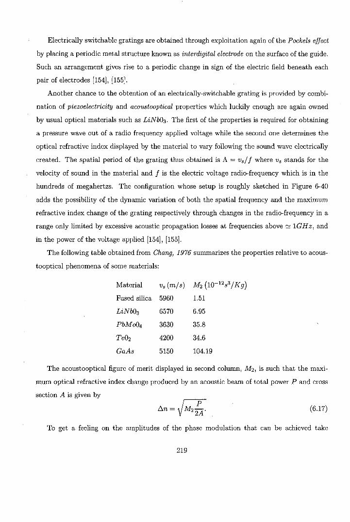
IIIIIIIIIIIIIIIIIIIII
Electrically switchable gratings are obtained through exploitation again of the Pockels effect
by placing a periodic metal structure known as interdigital electrode on the surface of the guide.
Such an arrangement gives rise to a periodic change in sign of the electric field beneath each
pair of electrodes [154], [155].
Another chance to the obtention of an electrically-switchable grating is provided by combi-
nation of piezoelectricity and acoustooptical properties which luckily enough are again owned
by usual optical materials such as LiNbO^. The first of the properties is required for obtaining
a pressure wave out of a radio frequency applied voltage while the second one determines the
optical refractive index displayed by the material to vary following the sound wave electrically
created. The spatial period of the grating thus obtained is A = vs/f where vs stands for the
velocity of sound in the material and / is the electric voltage radio-frequency which is in the
hundreds of megahertzs. The configuration whose setup is roughly sketched in Figure 6-40
adds the possibility of the dynamic variation of both the spatial frequency and the maximum
refractive index change of the grating respectively through changes in the radio-frequency in a
range only limited by excessive acoustic propagation losses at frequencies above ~ IGHz, and
in the power of the voltage applied [154], [155].
The following table obtained from Chang, 1976 summarizes the properties relative to acous-
tooptical phenomena of some materials:
Material vs (m/s) M2
Fused silica 5960 1.51
LiNbQs 6570 6.95
P6Mo04 3630 35.8
Te02 4200 34.6
GaAs 5150 104.19
The acoustooptical figure of merit displayed in second column, M2, is such that the maxi-
mum optical refractive index change produced by an acoustic beam of total power P and cross
section A is given by
To get a feeling on the amplitudes of the phase modulation that can be achieved take
219
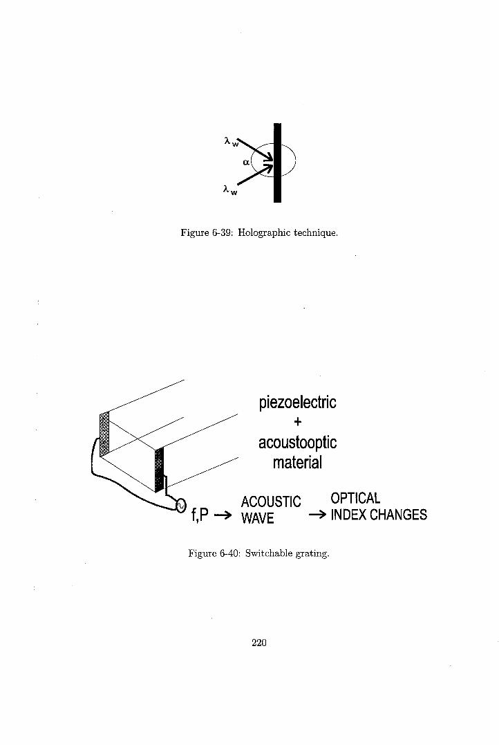
IIIIIIIIIIIIIIIIIIIII
Figure 6-39: Holographie technique.
piezoelectric
acoustoopticmaterial
ACOUSTIC OPTICALWAVE -> INDEX CHANGES
Figure 6-40: Switchable grating.
220

111
1111111
1
LiNbOs as an example and a reasonable total acoustic power of about P = IW applied upon
a rectangular cross sectional area giving a grating depth d = 1/nm and a y direction side
of I = 10/^m which is enough to cover the thin quadratic nonlinear waveguide. For a light
wavelength on the order of A ~ 1/̂ m one obtains
0 d 1 ,, P o /6-95 x 10~12
4>A -^Ay ¿ 2 ( d x l ) V 2 x l O ~ n (6.18)
but other values are also achievable through variation of the acoustic power or the cross sectional
area over which the stress is induced into the material.
As for an order of normalized spatial frequencies, the velocity of sound in LiNbQz, vs =
6570m/ s , gives for a radio-frequency of about / = 100MHz a spatial period of A = 65.7/^m
corresponding for rj — 15/^m to a normalized spatial frequency in the simulations of p ~ 0.23.
Well aware of the possibilities offered by input gratings, investigation of how the phase
modulation they inflict upon the input fields affects the solitary wave formation and propagation
inside the quadratically nonlinear waveguide is carried out in next section.
6.3.2 Analysis of input phase modulations
It has been shown that the net effect of placing a phase grating featuring a refractive index
distribution that varies sinusoidally in the transverse direction at the input face of the %(2)planar
guide is phase modulating the input beams. Following the usual notation for
fields in the x^ problem they can be expressed
of (s, £ = 0) = a¿ (s, Ç = 0) exp (—jíj)^ sin (27rp¿s + 0¿)) ,
the normalized
(6.19)
where the superindex distinguishes input fields with grating at the entrance face of the waveguide
1
1
1
1
1
1
1
from those in the absence of grating.
By using standard Bessel function expansion of the modulation term, the
also be expressed
m=oo
m=— oo
221
input fields can
(6.20)

IIIIIIIIIIIIIIIIIIIII
Such an initial beam distribution when propagating in a linear medium will result splitted up
in many subbeams travelling in different angles determined by tilts at multiples of the spatial
frequency of the grating, litpi each carrying a fraction of the total energy that depends on the
Bessel function of the order of the phase tilt multiplicity evaluated at the amplitude of the
phase modulation.
Conversely, in the quadratic nonlinear medium as a result of nonlinear interaction the energy
tends to gather in a single subbeam chosen through the dynamics depending both in input and
system parameters. The splitting up picture provided by the linear case renders useful however
to understand many of the features displayed by the nonlinear propagation.
In Figure 6-41 the colored lines while pointing in the direction followed by each subbeam
have modulus proportional to the fraction of initial energy they carry for a spatial frequency of
p = 0.2. As seen the higher the multiplicity of a given subbeam the faster it walks the z axis
off. Following the rule
^-m(^) = (-irJm(^). (6.21)
In the range of interest <f>Ai < 3.5, the amplitude of the rays going to the right in Figure
6-41 alternate in sign whereupon interfere destructively. Basically the distribution of energy
between the subbeams is characterized by a now of energy from the straight ray towards the
two first subbeams as <j>Ai increases until it is reached the <j)Ai ~ 2.4 value for which the two
first subbeams attract practically all the energy in equal shares such that no energy goes in
the straight direction. Above this value energy returns to the straight direction but now with
a negative amplitude and energy is transferred to higher multiplicity orders.
Figures 6-42 and 6-43 compare the characteristics of linear and nonlinear propagation show-
ing how helpful the linear picture results. Destructive interference of the subbeams at the right
hand side of the profiles causes the energy there to be dragged up towards more energetic left
hand side whose subbeams add up in constructive interference. When above 4>A. ~ 2.4 the
straight subbeam amplitude turns negative, the energy at the right hand side of the profiles
becomes more difficult to couple to the beam created by the constructive interference of the
subbeams at the left hand side and the net result is an increase in radiation to the right as the
<j)A. value is increased (Figure 6-44).
The transverse velocity with which the beam resulting from the nonlinear coupling among
222
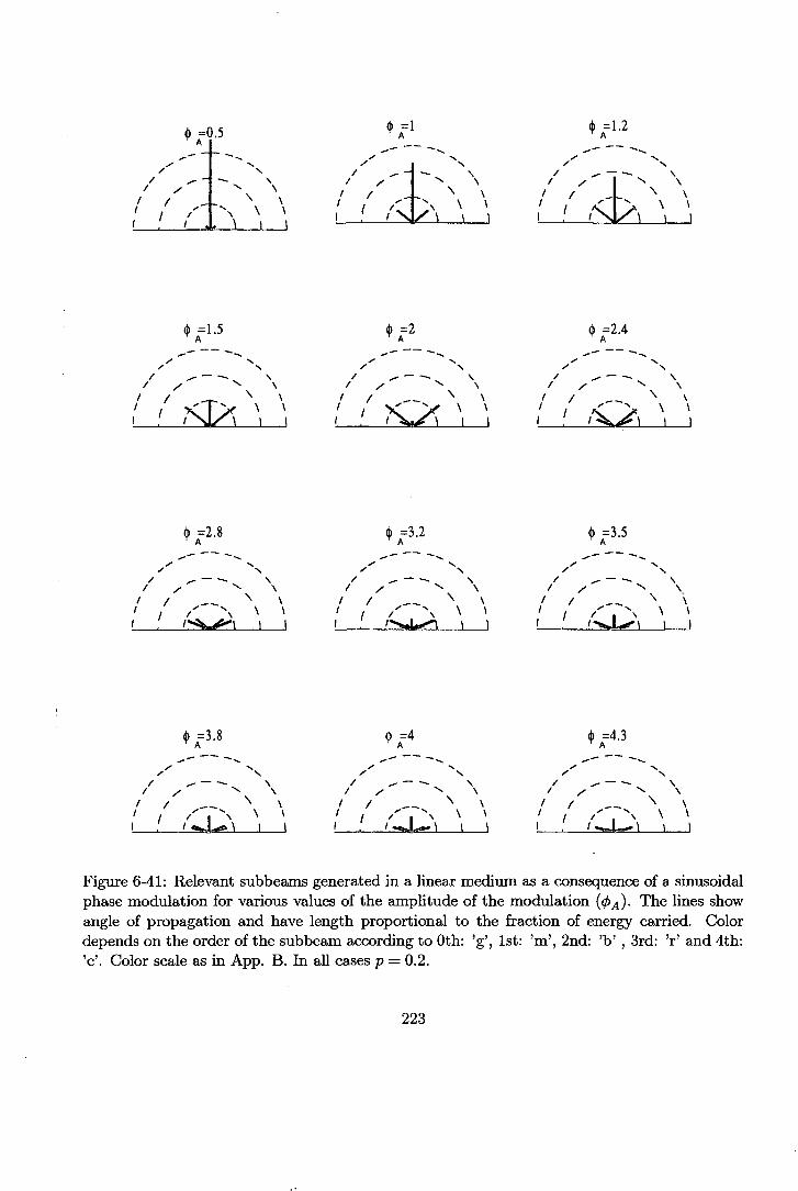
11™ 6 =0.5
T A
/ / \
I I . ' . . / ' , . \ 1 1
16 =1.5
1 -----• X V• X N
/ *̂ ' — — N' ' ^ ^ N
• / / N N1 ,' .' sl>; N, \
i|
è=2.8A
x xX N
• Í!^:<\ii
* =3.8
I ,"-::V;N/ x x \/ / . N \
I i .' //«wL·»N\ i i
6 =1 6 =1.2T A T A
'' A ^ /'~~ ^^
i ' x \ \ / x>-"r"v \ \/ /^ ^ i \. i ^ *i . i \ / \ i i i . i NJX\ i i
6 =2 è =2.4T A Y A
,'~~ ^""x /'' ^N/ ^f — <-̂ . \ / ^. — — ̂ \
/ X ^ N t / ~^ \1 / \ \ / / . . ^ \
<() =3.2 <|> =3.5T A T A
^ ^ s ^X N X s
/ ^ \ / ^ \/ X x \ ' / ^- \
/ / N \ / / . , N \
' ' '' NN N ^ / ' /Ci^ x v
6 =4 6 =4.3Y A T A
x xs x ^s/ ^- \ / ^- \/ x x \ / / x \
/ / N \ / / N \/ 1 ,' ^N \ \ / / /' v
s \ \
1 Figure 6-41: Relevant subbeams generated in a linear medium as a consequence of a sinusoidalphase modulation for various values of the amplitude of the modulation (0^). The lines showangle of propagation and have length proportional to the fraction of energy carried. Color
•depends on the order of the subbeam according to Oth: 'g', 1st: 'm', 2nd: 'b' , 3rd: 'T' and 4th:'c'. Color scale as in App. B. In all cases p = 0.2.
1
1
1
I
223

TIIIIIIIIIIIIIIIIIIII
-20 -10 0 10s: transverse coordinate
20 30
Figure 6-42: Linear ('black'-.) and nonlinear ( 'red'- ) propagation of the fundamental field forthe set of parameters A\ — 4, A-¿ = 0, (f>A = 1.2, p = 0.2, /? = 3. Straight lines indicate thedirection of the subbeams in a linear medium.
-20 -10 0 10s: transverse coordinate
20 30
Figure 6-43: Same as in previous figure but for <j>A = 2.4.
224
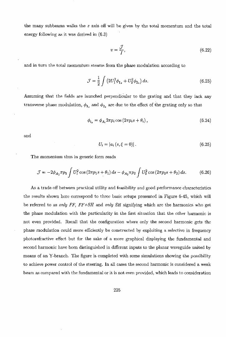
111111
11•
11
111
the many subbeams walks the z axis off will be given by the total momentum and
energy following as it was derived in (6.3)
v_J_
and in turn the total momentum steams from the phase modulation according to
H /(«**. -"«*.)«..
Assuming that the fields are launched perpendicular to the grating and that they
transverse phase modulation, </>ls and </>2s are due to the effect of the grating only so
fa* - ^Ai^pi cos (1-npiS + Oi] ,
and
Ui = |o¿(s,£ = 0)|.
The momentum thus in generic form reads
J = —1(j)A itp\ I U? cos (2?rpis + ¿M ds — <j>A~itp2 1 U% cos (l-np^s + 6-¿) ds.J J
the total
(6.22)
(6.23)
lack any
that
(6.24)
(6.25)
(6.26)
As a trade off between practical utility and feasibility and good performance characteristics
the results shown here correspond to three basic setups presented in Figure 6-45, which will
be referred to as only FF, FF+SH and only SH signifying which are the harmonics who get
the phase modulation with the particularity in the first situation that the other harmonic is
not even provided. Recall that the configuration where only the second harmonic gets the
phase modulation could more efficiently be constructed by exploiting a selective in frequency
photorefractive effect but for the sake of a more graphical displaying the fundamental and
second harmonic have been distinguished in different inputs to the planar waveguide united by
means of an Y-branch. The figure is completed with some simulations showing the possibility
to achieve power control of the steering. In all cases the second harmonic is considered a weak
beam as compared with the fundamental or it is not even provided, which leads to consideration
225

1111111111111
of positive wavevector mismatch configurations.
The expected velocity of the beams is obtained by calculating the
specific configuration
í 2¿JordyFF = 2(^^7Tp / [/} COS (2?TpS + 0) ds,
f 2 2^I^FF+SH — 20^717) / (t/i + C/2 ) c°s (2?rps + $) ds,
í 2¿îonlySH = UA^P / ^2 co^ (27TpS + 0) ds.
For the sech-like beams considered in the simulations, namely
Ui = AiSech(s),
C/2 = A2Slec/i(s) ,
the expected velocities in each case are
VonlyFF — ̂ A^P \ Seek? («) COS (2?TpS + 9) ds,
VFF+SH — ̂ A^P \ Sech (s) cos (2?rps + 0) ds,
(D A 7TÜJT.O / _, i 2 / \ /rv /»\71 i n r r / T j r t j r t r 7 l " i r*O" í TT1 rt 1 rî\ ft nuonlySH O / l 2 i 0/12 / oec'1 \S) COS (¿Tips -f- V) as.
6.3.3 Numerical experiments
momentum for each
(6.27)
(6.28)
(6.29)
(6.30)
(6.31)
(6.32)
(6.33)
(6.34)
First and second configurations as featuring a total independence of the transverse velocity upon
1
1
1
1
1
1
1
the initial amplitudes do not provide any chances for the power control of the steering if both
total momentum and total power in the system are perfectly conserved. Difficulties in reaching
the stationary amplitude relation when only launching the fundamental produce some energy
losses which due to the asymmetric phase profile imposed, mainly have transverse direction to
the right so that both the reduction of total energy and the increase in
finally carried by the soliton as a consequence of asymmetric radiation
the total momentum
thus produced cause
its speeding up towards the left. The effect is more pronounced for big values of the initial
226

away from the stationary amplitude values and hence the slight shift observed in Figure 6-45,
top row. The launching of the second harmonic as approaching the stationary values favours
the coupling of energy into the steered soliton while reducing the chances for power steering
control as seen in the plots in middle row.
Actual power steering control is therefore only achieved in third configuration with peak
deviations that reach 7 beam widths and power efficiencies on the 80% range (Figure 6-46).
The recurrent trade-off between maximum deviation and energy coupled to the soliton is also
here evident.
Because the calculated transverse velocities display explicit dependence upon the parameters
of the grating, i.e. p and </% the three configurations are in principle eligible for constituting
the basis for the building of setups in which the steering control in achieved by means of a
switchable grating.
Concerning optimum values of these two parameters, since the dependence upon (f)A is purely
proportional, for maximizing beam deviation one should want it to be as large as possible. On
the other side though, is energy lost during the evolution towards the stationary state which
is expected to grow. On the search for an optimum value it is useful to resort to the splitting
up linear picture (Figure 6-41). Negative sign for the amplitude of the straight beam above
(f)A ~ 2.4 as hindering the coupling of energy at the right hand side of the profile to the soliton
formed to the left produces an increase in radiation to the right which both enhances the soliton
deviation and reduces energy efficiency, just as the curves in Figure 6-47 show.
More complicated is the dependence upon the spatial frequency of the grating as appearing
also inside the integral. That an optimum value should exist is clear considering the sketch in
Figure 6-48.
Starting from a very low spatial frequency such that in the transverse interval corresponding
to relevant field amplitudes the phase modulation is viewed as a simple tilt, the calculated
transverse velocity increases as the spatial frequency does as in the pure linear tilt case provided
the most relevant part of the amplitude profile is sensible only to the negative slope of the
phase modulation. As the spatial frequency is increased till a portion of positive slope enters
the transverse area for relevant field amplitudes, the momentum should start to decrease.
For calculating such an optimum spatial frequency value find the derivative of the expression
227

for the transverse velocity with respect to p and equate to zero to get
/ Seek2 (s) (cos (2Trps) - 2Ttpsm (27rps)) ds = 0. (6.35)
This expression may be simplified using
---* sin (*) =E (-^^ (6-36)n=0
to give
2+ E í-1)" 7^)f
The ntegrals are found in the tables
í Seek2 (s) s*nds = 2 (22n - 2) (-V" \B2n\ , (6.38)
together with the property of Bernouilli numbers
B2n = (-I)""1 \Bin\ - (6.39)
Finally one obtains00 O _L 1
>- E («"-») ̂ sr (-'»')*'*" -° <M°)n=l ^ '
By using Boltzano approximation considering up to 10 terms in the summation, an optimum
value for the spatial frequency of the grating of p ~ 0.19 was obtained. Good accuracy of the
result was confirmed as further additions of terms of the summation modified the result at the
order of the third decimal digit.
The results in Figure 6-49 confirm the expectations for steering control with switchable
gratings, featuring a broad scanning range of about 20 beam widths for first and second con-
figurations and around 5 beam widths in third configuration with energy efficiencies of about
80%. Some examples of fields outputs obtained are shown in Figure 6-50.
Therefore if for power control of the steering the use of third configuration is advised, when
considering a switchable grating first and second configuration should be the choice for a greater
228

IIIIIIIIIIIIIIIIIIIII
range of angle scanning at the output of the waveguide.
Finally tolerances upon eventual variations of the wavevector mismatch or presence and
variation of a certain Poynting vector walk-off are briefly outlined with the aim of demonstrating
the robustness of the steering method here analyzed and its eligibility for constituting the basis
of practical setups, Figures 6-51, 6-52.
As the expected velocity as given by (6.22) only depends upon conserved quantities, the
wavevector mismatch dependence of the steering is determined by the behavior of radiation.
Thus, in top row of Figure 6-51 as only the fundamental field is launched, for moderate (3 values
the increase in Ii/I^STAT eases the initial momentum keeping and increases the steering with
energetic solitons. The exception are the ¡3 = 0 and ¡3 = 10 cases in which the enhancement of
the steering seems to come from prevailing radiation to the right as low energetic solitons are
produced.
Even when amplitude values close enough to the stationary ones are supplied in the third
setup considered, radiation is produced due to asymmetric A0 transverse distribution caused
by only the second harmonic to feel the phase distortion introduced by the input grating, hence
the soliton shifts displayed in bottom row.
In middle row instead, since both fundamental and second harmonic fields are launched
with amplitude values and relative phase values that ressemble the stationary ones, little effect
of radiation leads to almost independence of the soliton position with respect to the wavevector
mismatch value in the configuration.
As about presence of a certain Poynting vector walk-off as adding a new term for the
expected velocity with respect to (6.22), namely
« = y-«y, (6.41)
basically the tendency displayed is some deviation to the left when 6 > 0 and to the right when
6<0.
229

-20 -10 O 10s: transverse coordínate
20 30
Figure 6-44: Same as in Figure 6.42 but for <¡)A = 2.8.
230
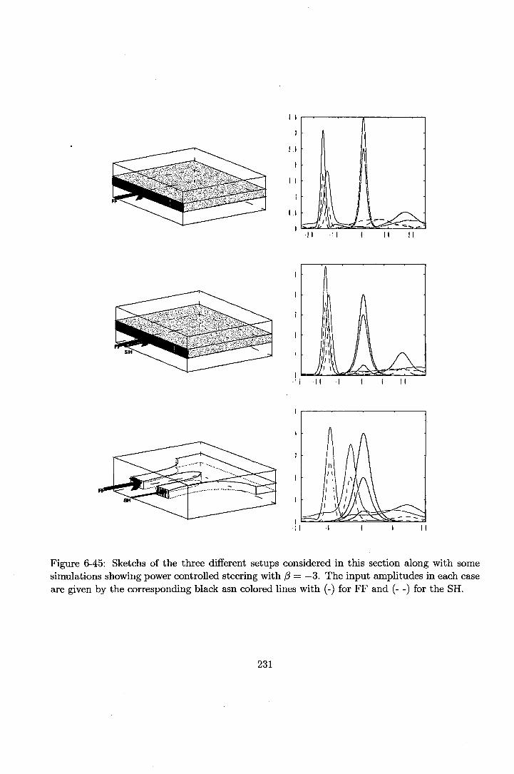
Il
Figure 6-45: Sketchs of the three different setups considered in this section along with somesimulations showing power controlled steering with (3 = —3. The input amplitudes in each caseare given by the corresponding black asn colored lines with (-) for FF and (- -) for the SH.
231
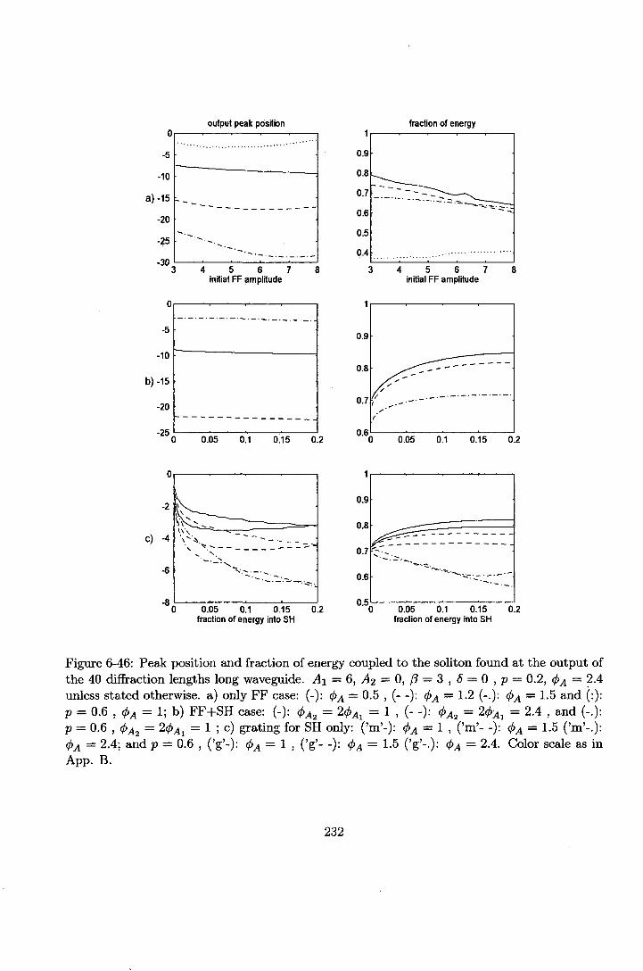
o
-5
-10
a)-15
-20
-25
-30 ;
O
-5
-10
b)-15
-20
-25
output peak position fraction of energy
4 5 6 7initial FF amplitude
0.9
0.8
0.7
0.6
0.5
0.4
0.05 0.1 0.15 0.2
0.9
0.8
0.7
0.6
4 5 6 7initial FF amplitude
0.05 0.1 0.15 0.2
-2
C) -4
-6
-80 0.05 0.1 0.15 0.2
fraction of energy into SH
1
0.9
0.8
0.7
0.6
0.50 0.05 0.1 0.15 0.2
fraction of energy into SH
Figure 6-46: Peak position and fraction of energy coupled to the soliton found at the output ofthe 40 diffraction lengths long waveguide. AI = 6, AZ = 0, /? = 3 , 6 = 0 , p = 0.2, <f>A = 2.4unless stated otherwise, a) only FF case: (-): <j)A = 0.5 , (- -): </>A — 1.2 (-.): </>A = 1.5 and (:):p = 0.6 , <t>A = 1; b) FF+SH case: (-): ̂ = 20Al = 1 , (- -): <^2 = 2j>-Al = 2.4 , and (-.):p = 0.6 , 0A2 = 2<f>Al = 1 ; c) grating for SH only: ('m'-): <j>A = 1 , ('m'- -): <f>A = 1.5 ('m'-.):
4>A = 2.4; and p = 0.6 , ('g'-): 0A = 1 , ('g'- -): 4>A = 1-5 ('g'--): ÏA = 2-4- Color scale «« inApp. B.
232

IIIIIIIIIIIIIIIIIIIII
OFTTTTT
1 2 3amplitude of the ph modulation
>.0.8E>O)
<U
o0.6cotí
•^0.4
0.21 2 3
amplitude of the ph modulation
Figure 6-47: Features of the steering dependence upon the amplitude of the phase modulation.In aU cases (3 = 3, p = 0.2, AÍ = 4. (-): only FF (-.): FF + SH A2 = 1, (:): only SH A2 = 1.
0.5
-0.5
-1
0.5
-10
-0.5
-110 -10 10 -10
-0.5
Figure 6-48: Illustrative of the dependence of the total momentum acquired by the beam onthe spatial frequency of the input grating.
233

output peak position
-5
a)-10
-15
-200 0.2 0.4 0.6 0.8 1
1
0.9
0.8
0.7
0.6
0.5
0.4
0.3
fraction of energy
0.2 0.4 0.6 0.8 1
0
-5
-10
b)-15
-20
-25
1
0.8
0.6
0.4
0.2
0 0.2 0.4 0.6 0.8 1 0 0.2 0.4 0.6 0.8 1
1
0
-1
C) -2
-3
-4
-50 0.2 0.4 0.6 0.8 1
spatial frequency
0.650.2 0.4 0.6 0.8 1
spatial frequency
Figure 6-49: Peak position and fraction of energy coupled to the soli ton found at the output ofthe 40 diffraction lengths long waveguide. AI = 4, A-¿ = I, (3 = 3 , 6 — 0 , p = 0.2, <¡>A = 2.4unless stated otherwise, a) only FF input case: (-): A\ = ^ <j>A = 0.5, (- -): A\ = 6, <f>A = 0.5,(-.): A! =4,<f>A = 1.5 b) FF+SH case: <^2 - 20Al = 1, (-): Aj = 4, A2 = 1, (- -): Al = 6,Ai = 1.5, (-.):Ai = 8, AI = 2, and (:): <f>M = 2^Al = l, AI = 4, A2 = 1; c) grating for SHonly: ('m'-): <f>A = 0.5, ('m'- -): <t>A = 1, ('m'-.): 0¿ = 1.5 ('g'-): 0A = 2.4, ('g'- -): ̂ = 3,('g'--): <t>A — 3-8- Color scale as in App. B.
234

IIIIII•
IIIIIIIIIIIIII
p as control
-2
-2
- 2 0 2s: transverse coordinate
6 8 10
6 8 10
6 8 10
Figure 6-50: Input and outputs of a 20 diffraction lengths waveguide (40 diffraction lengths foronly SH results) for the three setups considered showing steering control through the switchablegrating. Unless stated otherwise AI = 4, A2 — 1, ft = 3. ('m'): p = 0.1, ('g'): P = 0.2, ('r'):p = 0.3, ('b'): p = 0.4. Top: (f>A — 0.5, middle: <f>A = 1, bottom: <j>A = 2.4. Black thick linesshow the input field amplitudes with (-) for FF and (- - ) for SH. Color scale as in App. B.
235

IIIIIIIIIIIIIIIIIIIII
P dependence
- 2 0 2s: transverse coordinate
10
Figure 6-51: Input and outputs of a 20 diffraction lengths waveguide (40 diffraction lengthsfor only SH results) for the three setups considered showing dependences of the steering effectupon the wavevector mismatch. Unless stated otherwise AI = 4, AI = 1, p = 0.2, 0^ = 2.4.('m'): ft = O, ('g'):/? = 1, ('bk'): 0 = 3, ('r'): 0 = 6, ('b'): 0 = 10. Black thick lines show theinput field amplitudes with (-) for FF and (- - ) for SH. Color scale as in App. B.
236

IIIIIIIIIIIIIIIIIIIII
6 dependence
-10 - 5 0 5s: transverse coordinate
Figure 6-52: Input and outputs of a 20 diffraction lengths waveguide (40 diffraction lengthsfor only SH results) for the three setups considered showing dependences of the steering effectupon the wavevector mismatch. Unless stated otherwise AI = 4, AI = I , p = 0.2, (j)A = 2.4.(3 = 3 ('m'): S = -1.5, ('g'): S = -1, ('g'): à = -0-5, ('bk'): S = 0, (V): 6 = 0.5, (Y): S = 1.5.Black thick lines show the input field amplitudes with (-) for FF and (- - ) for SH. Color scaleas in App. B.
237

6.4 Power dependent splitting
The complicated dynamics undergone by fundamental and second harmonic fields once launched
into the quadratic material determines under certain circumstances total beam break up of the
input beams. That effect already outlined in section 3.6.3 will in the present section be analyzed
in detail. Beam break up produced by initial <j60 = TT differences was already explained section
6.2 and therefore the present section shall concentrate on splitting encountered with in phase
input beams.
Along with extensive numerical simulations demonstrating the effect, a simple picture that
qualitatively describes the mechanism causing the splitting and elucidates dependences upon
system and input parameters is derived. Emphasis is lied in practical application building
aspects and some hints to the design of practical setups that exploit the properties of the
splitting effect are given.
Recalling the analysis of the dynamics in section 3.6.3, when launching into the waveguide
bright profiles whose peak values for each harmonic resemble those for the stationary solution,
since initially nonlinear interaction prevails over diffraction, the beams peak will reach the
A0 ~ 0 nonlinear phase locking around a local energy value which is higher than required
taking into account the total energy contained in the beam in other words, the locking is
achieved with a transverse characteristic that is sharper than the one of the stationary solution
corresponding to the value of the peaks. That causes the beams to evolve into an oscillating
state in which through the focusing and defocusing periods undergone the peak results locked
to slightly higher local energy values reducing the variation in every period.
A quite distinct situation is encountered when initially diffraction prevails over nonlinear
interaction. In this case the beams peak may achieve the locking A(/> ~ 0 with local energy values
which are lower than the corresponding to the total energy in the beams. The A</> deviation
from locking brought about during the focusing period will thus be too slowly recovered by the
peak allowing during subsequent defocusing, a great deal of energy escape towards the profile
tails. The locking will then take place with a lower local energy value in peak whereupon a net
injection of energy towards the profile tails is set up which eventually allows for formation of
two solitons at each side of the center.
For total beam break-up therefore what it is needed is an initial reduced contribution of
238
11111
111111111111111
nonlinear interaction terms that keeps the beams peak from achieving the nonlinear phase
locking long enough for significant effect of diffraction to take place.
That condition has been found to be verified either by only injecting the fundamental in
which case as seen in section 3.6.2, initially A</> ~ — ?r/2 so that, in A0t only linear terms are
relevant, recall (3.88)
TT 1 TT 7T2\J I c e JL C/2 s s {J i
fa m i 1- V/ /n. t~*f~\C f j^k. /Al fí"^*"1 I /\ A\ 1 1 M — 0 1 fi /I O i
ç C/i 4 C/2 í/2
or else by injecting a very weak fundamental beam whereupon a very small UfUz product re-
duces the initial energy exchange velocity and hence that of nonlinear phase matching achieve-
ment.
Further initial detachment form phase locking condition takes place in the first case when a
negative /3 is considered, whereas in second case since energy exchange from second harmonic
to fundamental is required and then A</> > 0, the splitting is found in positive (3 configurations.
See the examples in Figure 6-53.
The first case, i.e. exclusive injection of the fundamental field, characterized by initial
total absence of nonlinear interactions (see (6.42)), is the one allowing for splitting in /3 — 0
configurations whereas contribution of the third term in (6.42) eases quick peak equilibrium
recovering and avoids splitting. The position of peaks found at the output of a 40 diffraction
lengths waveguide along with the energy coupled to each beam is plotted in Figure 6-54 showing
neat three soliton formation with little losses due to radiation and a neat switching effect around
AI ~ 5.5 corresponding to a normalized power of about I ~ 60.While the fields evolution in
Figure 6-53 c) seems to clearly respond to the splitting mechanism just explained, the quick
and well defined beam separation in d) seems to be due to a different effect.
The splitting shown in 6-53 c) which will be generically referred to as smooth splitting occurs
between two energy bounds and for low |/?| values following the mechanism explained above,
see Figures 6-57-6-58. The lower energy bound can intuitively be connected with quick enough
phase locking condition reaching in center so that it occurs in the period when diffraction
prevails over nonlinear interaction. As energy is increased, nonlinear interaction can be fast
enough so that it manages to counterbalance diffraction before the locking takes place thus
239

IIf
il
IIIIIIIIII
N 10
0
' 10
-10
-10
10
10
-10 " 0 10s: transverse coordinate
-10 0 10s: transverse coordinate
Figure 6-53: Examples of beam splitting. In all cases the fundamental beam evolution is shown,a) ,8 = -1. AI = 6.5. AI = 0;. b) (3 = 0, AI = 5, A-2 = 0; cV 3 = -2". A! = 6.5, A-2 = 0: d)(3 = -2, AI - 10, A'2 ='0; e ) ¿ = 3, Al - O.L A_> = 4; f) ,'d = 6. AI =0.1. .4,. = Ü. '
I 240

preventing the splitting for power values above a certain threshold.
The splitting occurring for higher |/3| values and high input powers and that gives rise to
great separation between the two solitons produced at the very firsts steps of the propagation,
hereafter referred to as sharp splitting, can be shown to respond to a somewhat different
mechanism which involves consideration of lateral bumps creation which was discussed in the
dynamics section. See Figures 6-55-6-56.
For very high \/3\ values as strongly determining a A<^> value monotonie evolution, even
transverse points containing significant amounts of local energy are likely to get stuck around
a cos (A0) < 0 area whereupon the nonlinear negative contribution to the phases causes the
energy in those points to result washed away towards other transverse points in the profile.
This effect is related to the increase of radiation produced as a consequence of larger difference
between the stationary solution and the initial conditions considered here as the |/?| value is
increased.
For high energy values, too sharp transverse profile stationary solution requirements for
peak, further desequilibrated from its phase locking condition due to energy dragged from
amplitude valley, hinders balanced oscillation state formation in center. On the other hand
in the profile 'tails' where the energy received from the amplitude valley is helping to achieve
the phase locking condition, as featuring lower peak amplitude values, the stationary solution
transverse profile requirements result greatly loosened down so that they more easily form a
soliton.
The differences between the two classes of splitting are evidenced in Figures 6-59 and 6-60
featuring the A<?!> evolution in a transverse point close to center for smooth and sharp splitting
cases. The plots show that sharp splitting is characterized by significant injection of energy
into the peak taking place when fairly close to center profile points undergo cos (A0) < 0 values
which immediately and unrelentlessly lead to the splitting.
One might think then that if energy is increased further even half the energy alloted to each
lateral bump should require too sharp and hence each lateral bump must split up into other
two as it is actually also seen to happen, Fig. 6-55.
Despite being produced through a quite messy dynamics evolution with energy being strug-
gled back and forth between wings and center, fairly neat solitons emerge from the beam
241

IIIIIIIIIIIIIIIIIIIII
breaking up with detachments from center that go from 5 to 20 beam widths. Energy efficien-
cies are within reasonable ranges, in all cases about 30% of the input energy is alloted to each
soliton, allowing to think in interesting practical applications.
The effect for negative ft of a weak slightly tilted signal beam was investigated yielding
the result in Figure 6-61 As seen, both the number of solitons produced as well as the energy
coupled to each can be controlled through control of the tilt angle of the small second harmonic
signal.
40
30
20
10
peaks position fraction of energy into each soliton
<]*p=o
-10
-20
-30
-40
o,*<
00003)
5 6 7initial FF amplitude
4 5 6 7initial FF amplitude
Figure 6-54: Position of the peaks found at the output of a 40 diffraction lengths waveguide(left) and fraction of input energy coupled to it (right) as a function of the input fundamentalamplitude. Here (3 = 0 and the second harmonic is not provided, i.e. A-¿ = 0.
242

IIIIIIIIIIIIIIIII1III
peaks position
B=-3
0.5
0.4
0.3
i0.2
0.1I
fraction of energy into each soliton
t. ».«
<«<;>i
10 12 14 16 18 20OS»î88ffl«BM<10 12 14 18 20
B=-4
20
10
-10
-20
* * **%
* * O3o o
9Q
.o on °
10 12 14 16initial FF amplitude
0.5
0.45
0.4
0.35'
0.3
0.25
0.2
0.15
O
o o
10 12 14 16initial FF amplitude
Figure 6-55: Same as Figure 6-54 but for f3 = — 3 (top) and /? = —4 (bottom).
243
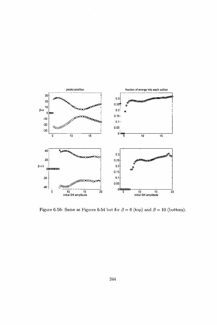
IIIIIIIIIIIIIIIIIIIII
peaks position fraction of energy into each soliton
10 15 10 15
P=10
40
20
I0
-20
-40 $ZW$$$^
5 10 15initial SH amplitude
20
0.3
0.25
0.2
0.15
0.1
0.05
Os10 15
initial SH amplitude20
Figure 6-56: Same as Figures 6-54 but for /? = 6 (top) and /? = 10 (bottom).
244

IIIIIIIIIIIIIIIIIIIII
10
5
P=-l
-5
-10
20
10
P=-2o
-10
-20
peaks position
J**
O
OCQ
O
*10 12 14 16 18initial FF amplitude
fraction of energy into each soliton
0.6
0.5(
0.4
0.3
0.2
0.1
-4f**«-
0.8
0.6
0.4
<0.2
0
00
o
10 12 14 16 18initial FF amplitude
Figure 6-57: Same as Figure 6-54 but for /? = — 1 (top) and /3 = —2 (bottom).
245

peaks position fraction of energy into each soliton
p=3
10
5
-5
10
* #
*
0°°°ooooo0
0.6
0.5
0.4
0.3
0.2
0.1
0 oooooooooç0°
. ®<8®®®®®«®
2 3 4 5 6 7 2 3 4 5 6 7
on
10
Oí
10
in
*********%
****** *
$888 8 ®»®C»«®«(0 0
0̂0°°°°QoocccCDC^
0.6
0.5
0.4
0.3
0.2
0.1
rv
gg®W "̂
9
^ <
2 4 6initial SH amplitude
2 4 6initial SH amplitude
Figure 6-58: Same as Figures 6-54 but for (3 = 2 (top) and (3 = 3 (bottom).
246

smooth splitting, A1=6.5, m: s=0.5, g: s=1.3 sharp splitting, A1=10, m: s=0.5, g: s=1.3
-0.5
-1-1.6
-2-2.5
-3-3.5
5 10z: propagation variable
15
200
>.150
S>cœ100au^ 5 0
2 4z: propagation variable
Figure 6-59: Nonlinear phase mismatch and local energy evolution, top and bottom rows respec-tively, in different transverse points: ('bk'): peak; ('m'): \s\ = 0.5; ('g'): \s\ = 1.3; illustratingthe differences between smooth and sharp splitting, respectively at left AI = 6.5, and at rightAI = 10. In all cases ¡3 = —2, A-¿ = 0. Color scale as in App. B.
247
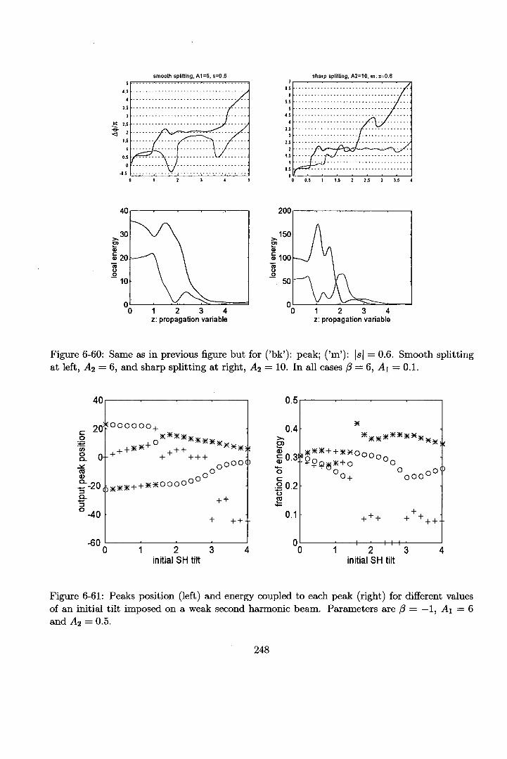
1111111
O>O)
I In00
1
1
smooth splitting, A 1=6, s=0.6 sharp splitting, A2=10, m: $=0.6
4.5 •-/
25 >^\ ̂ ^-^—^^ "f\ "^Vx-~^ ^^ -^
'f C \ /1 ^^'^~^\ I \y"•* f \ /
ft g V
6 5 f •
I
5 —^
/^\ X
3.5 -/-
s y2 5 /\ /v>-V >^
,/c^3~^^*^Ü.5 *-*
0 1 2 3 4 5 0 0.5 1 1.5 2 2.5 3 3.5 4
40 inn
30 "\/\\\
20— ̂ ^y \
10 \ \
>,150 /\O) / i(p I \ /\i loo— ̂ y \
50 "~ \̂ V \
v^V-W-^0 1 2 3 4 0 1 2 3 4
z: propagation variable z: propagation variable
Figure 6-60: Same as in previous figure but for ('bk'): peak; ('m'): \s\ = 0.6. Smooth splitting_ at left, AI = 6,
An*TW
1 do
1 I ° - + jmo>
|t-200*>
f°-40
|0
1
and sharp splitting at right, A¿ = 10. In all cases (3 = 6, AI = 0.1.
n c
D O O O O +
3K ^^5K3^5|x>|,
h + ** + + + 5K^$
0OK5K + + ; iK^OOOO 0
U.O ' ' '
0.4 *>» 3K3K^ ^ 3K^vi/
; |o.3l|^+;^°oo00o 'Ao O „. O nOc O+ QOO U
|02
^ 0.1 • + + + + + + -
1 2 3 4 "O 1 ' 2 ' ' ' 3 4initial SH tilt initial SH tilt
1Figure 6-61: Peaks position (left) and energy coupled to each peak (right) for different valuesof an initial tilt imposed on a weak second harmonic beam. Parameters are /3 = —1, AI = 6and A-i = 0.5.
1
1
1
1
248