Optical properties of Semiconductor Nanostructures:

Decoherence versus Quantum Control

Ulrich Hohenester

Institut fur Physik, Theoretische PhysikKarl–Franzens–Universitat GrazUniversitatsplatz 5, 8010 Graz, Austria

Phone: +43 316 380 5227Fax: +43 316 380 9820www: http://physik.uni-graz.at/∼uxh/

email: ulrich.hohenester@uni-graz.at

to appear in “Handbook of Theoretical and Computational Nanotechnology”

1

Contents

1 Introduction 4

2 Motivation and overview 5

2.1 Quantum confinement . . . . . . . . . . . . . . . . . . . . . . . . . 5

2.2 Scope of the paper . . . . . . . . . . . . . . . . . . . . . . . . . . 7

2.3 Quantum coherence . . . . . . . . . . . . . . . . . . . . . . . . . . 8

2.4 Decoherence . . . . . . . . . . . . . . . . . . . . . . . . . . . . . . 10

2.5 Quantum control . . . . . . . . . . . . . . . . . . . . . . . . . . . 11

2.6 Properties of artificial atoms . . . . . . . . . . . . . . . . . . . . . 12

3 Few-particle states 14

3.1 Excitons . . . . . . . . . . . . . . . . . . . . . . . . . . . . . . . . 16

3.1.1 Semiconductors of higher dimension . . . . . . . . . . . . . 16

3.1.2 Semiconductor quantum dots . . . . . . . . . . . . . . . . . 17

3.1.3 Spin structure . . . . . . . . . . . . . . . . . . . . . . . . . 20

3.2 Biexcitons . . . . . . . . . . . . . . . . . . . . . . . . . . . . . . . 23

3.2.1 Weak confinement regime . . . . . . . . . . . . . . . . . . . 24

3.2.2 Strong confinement regime . . . . . . . . . . . . . . . . . . 24

3.3 Other few-particle complexes . . . . . . . . . . . . . . . . . . . . . 25

3.4 Coupled dots . . . . . . . . . . . . . . . . . . . . . . . . . . . . . . 27

4 Optical spectroscopy 28

4.1 Optical absorption . . . . . . . . . . . . . . . . . . . . . . . . . . . 31

4.1.1 Weak confinement . . . . . . . . . . . . . . . . . . . . . . . 32

4.1.2 Strong confinement . . . . . . . . . . . . . . . . . . . . . . 33

4.2 Luminescence . . . . . . . . . . . . . . . . . . . . . . . . . . . . . 34

4.3 Multi and multi-charged excitons . . . . . . . . . . . . . . . . . . . 36

4.4 Near-field scanning microscopy . . . . . . . . . . . . . . . . . . . . 38

4.5 Coherent optical spectroscopy . . . . . . . . . . . . . . . . . . . . . 40

5 Quantum coherence and decoherence 41

5.1 Quantum coherence . . . . . . . . . . . . . . . . . . . . . . . . . . 41

5.1.1 Two-level system . . . . . . . . . . . . . . . . . . . . . . . 42

5.2 Decoherence . . . . . . . . . . . . . . . . . . . . . . . . . . . . . . 45

5.2.1 Caldeira-Leggett-type model . . . . . . . . . . . . . . . . . 46

5.2.2 Unraveling of the master equation . . . . . . . . . . . . . . 48

5.3 Photon scatterings . . . . . . . . . . . . . . . . . . . . . . . . . . . 49

5.4 Single-photon sources . . . . . . . . . . . . . . . . . . . . . . . . . 53

2

5.5 Phonon scatterings . . . . . . . . . . . . . . . . . . . . . . . . . . 59

5.5.1 Spin-boson model . . . . . . . . . . . . . . . . . . . . . . . 59

5.6 Spin scatterings . . . . . . . . . . . . . . . . . . . . . . . . . . . . 64

6 Quantum control 65

6.1 Stimulated Raman adiabatic passage . . . . . . . . . . . . . . . . . 67

6.2 Optimal control . . . . . . . . . . . . . . . . . . . . . . . . . . . . 70

6.3 Self-induced transparency . . . . . . . . . . . . . . . . . . . . . . . 78

7 Quantum computation 80

A Rigid exciton and biexciton approximation 83

A.1 Excitons . . . . . . . . . . . . . . . . . . . . . . . . . . . . . . . . 83

A.2 Biexcitons . . . . . . . . . . . . . . . . . . . . . . . . . . . . . . . 84

A.3 Optical dipole elements . . . . . . . . . . . . . . . . . . . . . . . . 84

B Configuration interactions 85

B.1 Second quantization . . . . . . . . . . . . . . . . . . . . . . . . . . 85

B.2 Direct diagonalization . . . . . . . . . . . . . . . . . . . . . . . . . 86

B.2.1 Excitons . . . . . . . . . . . . . . . . . . . . . . . . . . . . 87

B.2.2 Biexcitons . . . . . . . . . . . . . . . . . . . . . . . . . . . 87

C Two-level system 88

D Independent boson model 90

3

1 Introduction

Although there is a lot of quantum physics at the nanoscale, one often has to

work hard to observe it. In this review we shall discuss how this can be done for

semiconductor quantum dots. These are small islands of lower-bandgap material

embedded in a surrounding matrix of higher-bandgap material. For properly chosen

dot and material parameters, carriers become confined in all three spatial directions

within the low-bandgap islands on a typical length scale of tens of nanometers. This

three-dimensional confinement results in atomic-like carrier states with discrete en-

ergy levels. In contrast to atoms, quantum dots are not identical but differ in size

and material composition, which results in large inhomogeneous broadenings that

usually spoil the direct observation of the atomic-like properties. Optics allows to

overcome this deficiency by means of single-dot or coherence spectroscopy. Once

this accomplished, we fully enter into the quantum world: the optical spectra are

governed by sharp and ultranarrow emission peaks — indicating a strong suppres-

sion of environment couplings. When more carriers are added to the dot, e.g. by

means of charging or non-linear photoexcitation, they mutually interact through

Coulomb interactions which gives rise to intriguing energy shifts of the few-particle

states. This has recently attracted strong interest as it is expected to have profound

impact on opto-electronic or quantum-information device applications. A detailed

theoretical understanding of such Coulomb-renormalized few-particle states is there-

fore of great physical interest and importance, and will be provided in the first part

of this paper. In a nutshell, we find that nature is gentle enough to not bother

us too much with all the fine details of the semiconductor materials and the dot

confinement, but rather allows for much simpler description schemes. The most

simple one, which we shall frequently employ, is borrowed from quantum optics

and describes the quantum-dot states in terms of generic few-level schemes. Once

we understand the nature of the Coulomb-correlated few-particle states and how

they couple to the light, we can start to look closer. More specifically, we shall

show that the intrinsic broadenings of the emission peaks in the optical spectra

give detailed information about the way the states are coupled to the environment.

This will be discussed at the examples of photon and phonon scatterings. Optics

can do more than just providing a highly flexible and convenient characterization

tool: it can be used as a control, that allows to transfer coherence from an external

laser to the quantum-dot states and to hereby deliberately set the wavefunction of

the quantum system. This is successfully exploited in the fields of quantum control

and quantum computation, as will be discussed in detail in later parts of the paper.

The field of optics and quantum optics in semiconductor quantum dots has

recently attracted researchers from different communities, and has benefited from

4

their respective scientific backgrounds. This is also reflected in this paper, where we

review genuine solid-state models, such as the rigid-exciton or independent-boson

ones, as well as quantum-chemistry schemes, such as configuration interactions

or genetic algorithms, or quantum-optics methods, such as the unraveling of the

master equation through “quantum jumps” or the adiabatic population transfer.

The review is intended to give an introduction to the field, and to provide the

interested reader with the key references for further details. Throughout, I have

tried to briefly explain all concepts and to make the manuscript as self-contained as

possible. The paper has been organized as follows. In sec. 2 we give a brief overview

of the field and introduce the basic concepts. Section 3 is devoted to an analysis of

the Coulomb-renormalized few-particle states and of the more simplified few-level

schemes for their description. How these states can be probed optically is discussed

in sec. 4. The coherence and decoherence properties of quantum-dot states are

addressed in sec. 5, and we show how single-photon sources work. Finally, secs. 6

and 7 discuss quantum-control and quantum-computation applications. To keep

the paper as simple as possible, we have postponed several of the computational

details to the various appendices.

2 Motivation and overview

2.1 Quantum confinement

The hydrogen spectrum

εn = −E0

n2, n = 1, 2, . . . . (1)

provides a prototypical example for quantized motion: only certain eigenstates char-

acterized by the quantum number n (together with the angular quantum numbers `

andm`) are accessible to the system. While the detailed form is due to the Coulomb

potential exerted by the nucleus, eq. (1) exhibits two generic features: first, the

spectrum εn is discrete because the electron motion is confined in all three spatial

directions; second, the Rydberg energy scale E0 = e2/(2a0) and Bohr length scale

a0 = ~2/(me2) are determined by the natural constants describing the problem,

i.e. the elementary charge e, the electron mass m, and Planck’s constant ~. These

phenomena of quantum confinement and natural units prevail for the completely

different system of semiconductor quantum dots. These are semiconductor nanos-

tructures where the carrier motion is confined in all three spatial directions [1, 2, 3].

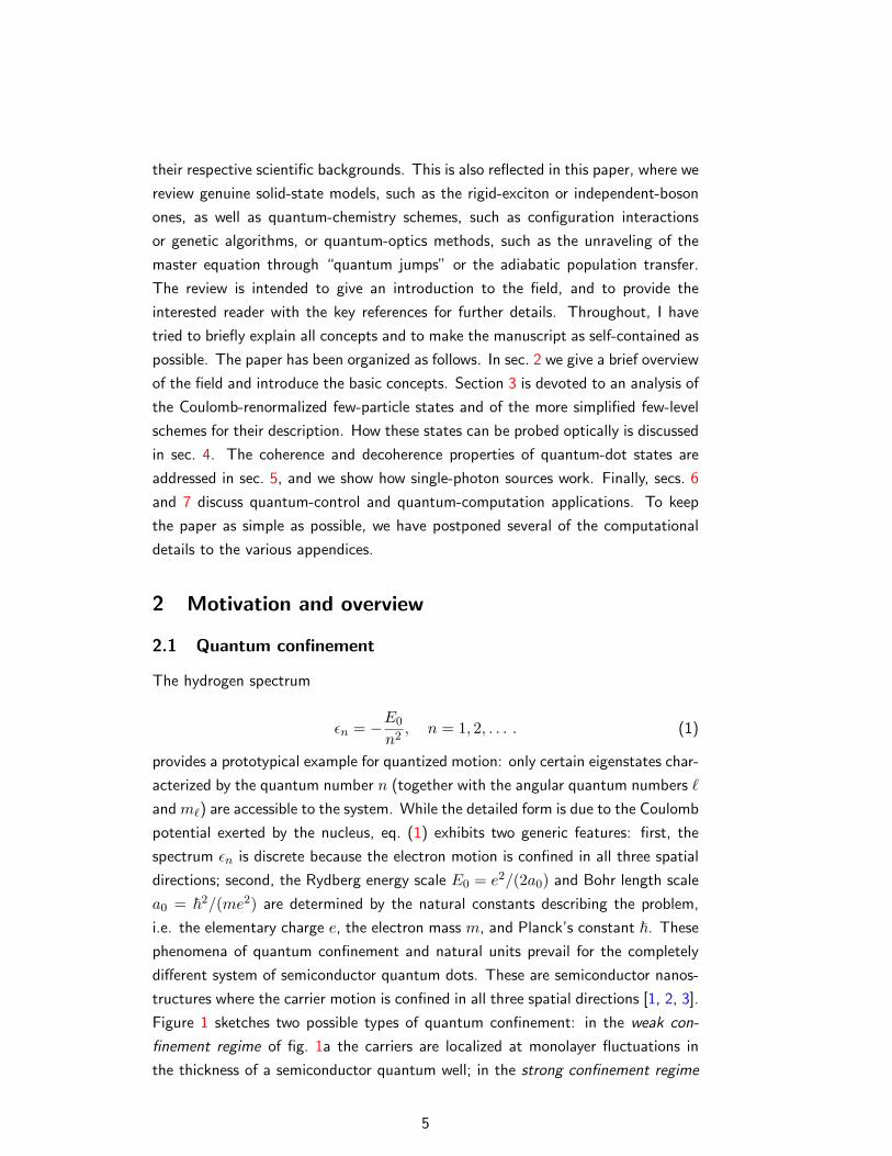
Figure 1 sketches two possible types of quantum confinement: in the weak con-

finement regime of fig. 1a the carriers are localized at monolayer fluctuations in

the thickness of a semiconductor quantum well; in the strong confinement regime

5

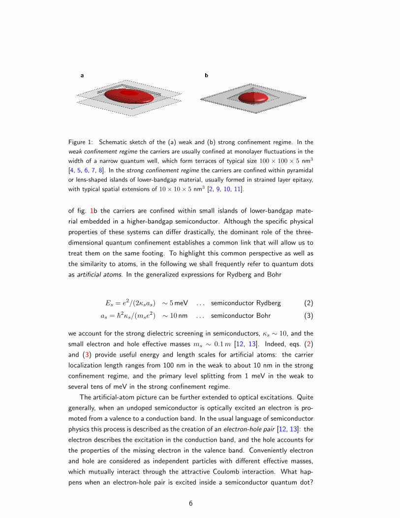
Figure 1: Schematic sketch of the (a) weak and (b) strong confinement regime. In the

weak confinement regime the carriers are usually confined at monolayer fluctuations in the

width of a narrow quantum well, which form terraces of typical size 100 × 100 × 5 nm3

[4, 5, 6, 7, 8]. In the strong confinement regime the carriers are confined within pyramidal

or lens-shaped islands of lower-bandgap material, usually formed in strained layer epitaxy,

with typical spatial extensions of 10× 10× 5 nm3 [2, 9, 10, 11].

of fig. 1b the carriers are confined within small islands of lower-bandgap mate-

rial embedded in a higher-bandgap semiconductor. Although the specific physical

properties of these systems can differ drastically, the dominant role of the three-

dimensional quantum confinement establishes a common link that will allow us to

treat them on the same footing. To highlight this common perspective as well as

the similarity to atoms, in the following we shall frequently refer to quantum dots

as artificial atoms. In the generalized expressions for Rydberg and Bohr

Es = e2/(2κsas) ∼ 5 meV . . . semiconductor Rydberg (2)

as = ~2κs/(mse2) ∼ 10 nm . . . semiconductor Bohr (3)

we account for the strong dielectric screening in semiconductors, κs ∼ 10, and the

small electron and hole effective masses ms ∼ 0.1m [12, 13]. Indeed, eqs. (2)

and (3) provide useful energy and length scales for artificial atoms: the carrier

localization length ranges from 100 nm in the weak to about 10 nm in the strong

confinement regime, and the primary level splitting from 1 meV in the weak to

several tens of meV in the strong confinement regime.

The artificial-atom picture can be further extended to optical excitations. Quite

generally, when an undoped semiconductor is optically excited an electron is pro-

moted from a valence to a conduction band. In the usual language of semiconductor

physics this process is described as the creation of an electron-hole pair [12, 13]: the

electron describes the excitation in the conduction band, and the hole accounts for

the properties of the missing electron in the valence band. Conveniently electron

and hole are considered as independent particles with different effective masses,

which mutually interact through the attractive Coulomb interaction. What hap-

pens when an electron-hole pair is excited inside a semiconductor quantum dot?

6

External fielde.g. laser

Systeme.g. atom or artificial atom

Environmente.g. photons

Measuremente.g. photo detection

Controle.g. laser pulse shaping

_v

_ _ _ _ _ _ _ _ _ _

6T

6

T _ _ _ _ _ _ _ _ _ __ v

//

Decoherenceoo

OO

OO

__

Objective function

?O U X Z \ b d f i p

Figure 2: Schematic representation of optical spectroscopy (shaded boxes) and quantum

control (dashed lines): an external field acts upon the system and promotes it from the

ground to an excited state; the excitation decays through environment coupling, e.g. photo

emission, and a measurement is performed indirectly on the environment, e.g. photo de-

tection. In case of quantum control the perturbation is tailored such that a given objective,

e.g. the wish to channel the system from one state to another, is fulfilled in the best way.

This is usually accomplished by starting with some initial guess for the external field, and

to improve it by exploiting the outcome of the measurement. The arrows in the figure

indicate the flow of information.

Things strongly differ for the weak and strong confinement regime: in the first case

the electron and hole form a Coulomb-bound electron-hole complex —the so-called

exciton [12]— whose center-of-mass motion becomes localized and quantized in

presence of the quantum confinement; in the latter case confinement effects dom-

inate over the Coulomb ones, and give rise to electron-hole states with dominant

single-particle character. However, in both cases the generic feature of quantum

confinement gives rise to discrete, atomic-like absorption and emission-lines — and

thus allows for the artificial-atom picture advocated above.

2.2 Scope of the paper

Quantum systems can usually not be measured directly. Rather one has to per-

turb the system and measure indirectly how it reacts to the perturbation. This

is schematically shown in fig. 2 (shaded boxes): an external perturbation, e.g. a

laser field, acts upon the quantum system and promotes it from the ground to

7

an excited state; the excitation decays through environment coupling, e.g. photo

emission, and finally a measurement is performed on some part of the environment,

e.g. through photo detection. As we shall see, this mutual interaction between

system and environment —the environment influences the system and in turn be-

comes influenced by it (indicated by the arrows in fig. 2 which show the flow of

information)— plays a central role in the understanding of decoherence and the

measurement process [14].

Optical spectroscopy provides one of the most flexible measurement tools since

it allows for a remote excitation and detection. It gives detailed information about

the system and its environment. This is seen most clearly at the example of atomic

spectroscopy which played a major role in the development of quantum theory and

quantum electrodynamics [15], and most recently has even been invoked in the

search for non-constant natural constants [16]. In a similar, although somewhat

less fundamental manner spectroscopy of artificial atoms allows for a detailed un-

derstanding of both electron-hole states (sec. 4) and of the way these states couple

to their environment (sec. 5). On the other hand, such detailed understanding

opens the challenging perspective to use the external fields in order to control the

quantum system. More specifically, the coherence properties of the exciting laser

are transfered to quantum coherence in the system, which allows to deliberately set

the state of the quantum system (see lower part of fig. 2). Recent years have seen

spectacular examples of such light-matter manipulations in atomic systems, e.g.

Bose-Einstein condensation or freezing of light (see, e.g. Chu [17] and references

therein). This tremendous success also initiated great stimulus in the field of solid-

state physics, as we shall discuss for artificial atoms in sec. 6. More recently, the

emerging fields of quantum computation [18, 19, 20] and quantum communication

[21] have become another driving force in the field. They have raised the prospect

that an almost perfect quantum control would allow for computation schemes that

would outperform classical computation. In turn, a tremendous quest for suited

quantum systems has started, ranging from photons over molecules, trapped ions

and atomic ensembles to semiconductor quantum dots. We will briefly review some

proposals and experimental progress in sec. 7.

2.3 Quantum coherence

Quantum coherence is the key ingredient and workhorse of quantum control and

quantum computation. To understand its essence, let us consider a generic two-

level system with ground state |0〉 and excited state |1〉, e.g. an artificial atom with

one electron-hole pair absent or present. The most general wavefunction can be

written in the form

8

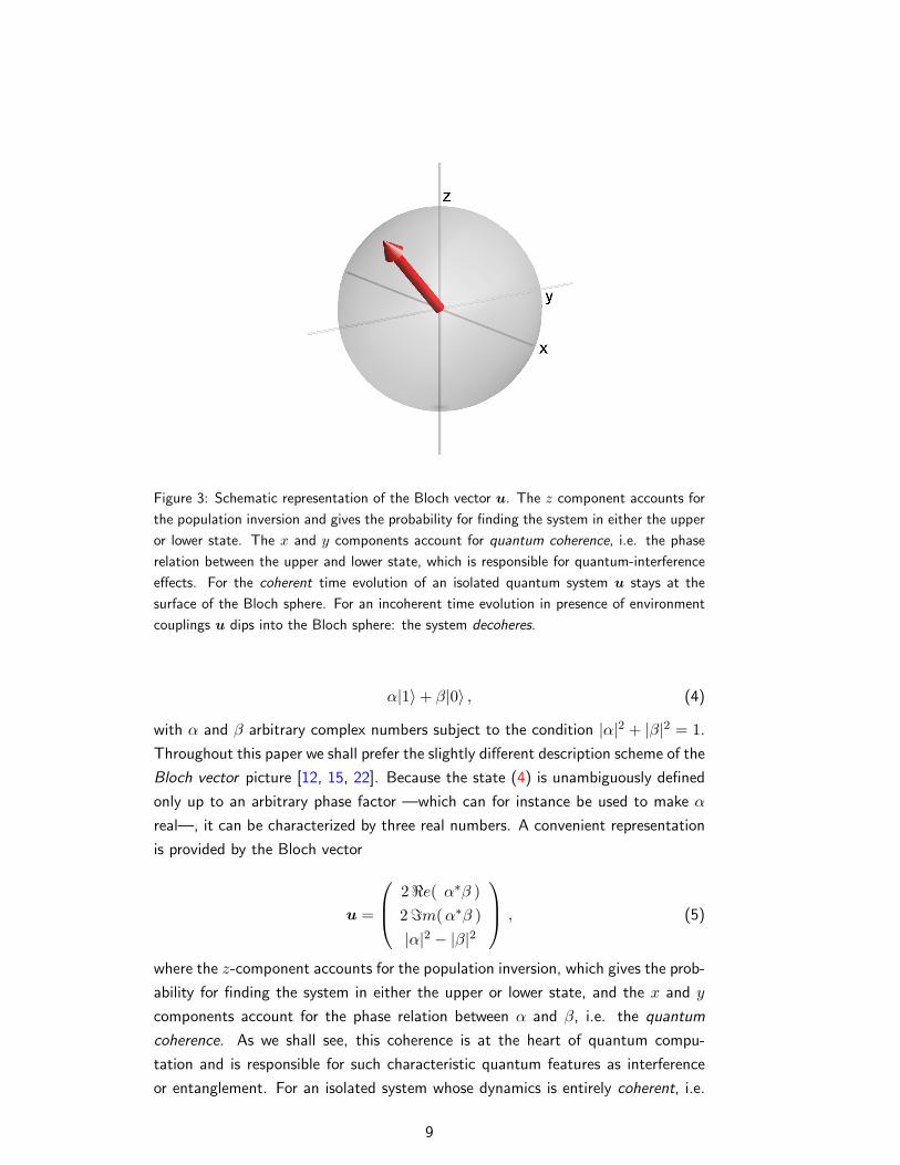
Figure 3: Schematic representation of the Bloch vector u. The z component accounts for

the population inversion and gives the probability for finding the system in either the upper

or lower state. The x and y components account for quantum coherence, i.e. the phase

relation between the upper and lower state, which is responsible for quantum-interference

effects. For the coherent time evolution of an isolated quantum system u stays at the

surface of the Bloch sphere. For an incoherent time evolution in presence of environment

couplings u dips into the Bloch sphere: the system decoheres.

α|1〉+ β|0〉 , (4)

with α and β arbitrary complex numbers subject to the condition |α|2 + |β|2 = 1.

Throughout this paper we shall prefer the slightly different description scheme of the

Bloch vector picture [12, 15, 22]. Because the state (4) is unambiguously defined

only up to an arbitrary phase factor —which can for instance be used to make α

real—, it can be characterized by three real numbers. A convenient representation

is provided by the Bloch vector

u =

2<e( α∗β )2=m(α∗β )|α|2 − |β|2

, (5)

where the z-component accounts for the population inversion, which gives the prob-

ability for finding the system in either the upper or lower state, and the x and y

components account for the phase relation between α and β, i.e. the quantum

coherence. As we shall see, this coherence is at the heart of quantum compu-

tation and is responsible for such characteristic quantum features as interference

or entanglement. For an isolated system whose dynamics is entirely coherent, i.e.

9

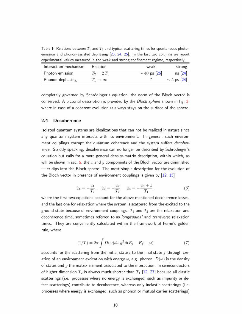
Table 1: Relations between T1 and T2 and typical scattering times for spontaneous photon

emission and phonon-assisted dephasing [23, 24, 25]. In the last two columns we report

experimental values measured in the weak and strong confinement regime, respectively.

Interaction mechanism Relation weak strong

Photon emission T2 = 2T1 ∼ 40 ps [26] ns [24]

Phonon dephasing T1 →∞ ? ∼ 5 ps [24]

completely governed by Schrodinger’s equation, the norm of the Bloch vector is

conserved. A pictorial description is provided by the Bloch sphere shown in fig. 3,

where in case of a coherent evolution u always stays on the surface of the sphere.

2.4 Decoherence

Isolated quantum systems are idealizations that can not be realized in nature since

any quantum system interacts with its environment. In general, such environ-

ment couplings corrupt the quantum coherence and the system suffers decoher-

ence. Strictly speaking, decoherence can no longer be described by Schrodinger’s

equation but calls for a more general density-matrix description, within which, as

will be shown in sec. 5, the x and y components of the Bloch vector are diminished

— u dips into the Bloch sphere. The most simple description for the evolution of

the Bloch vector in presence of environment couplings is given by [12, 15]

u1 = −u1

T2, u2 = −u2

T2, u3 = −u3 + 1

T1, (6)

where the first two equations account for the above-mentioned decoherence losses,

and the last one for relaxation where the system is scattered from the excited to the

ground state because of environment couplings. T1 and T2 are the relaxation and

decoherence time, sometimes referred to as longitudinal and transverse relaxation

times. They are conveniently calculated within the framework of Fermi’s golden

rule, where

(1/T ) = 2π∫D(ω)dω g2 δ(Ei − Ef − ω) (7)

accounts for the scattering from the initial state i to the final state f through cre-

ation of an environment excitation with energy ω, e.g. photon; D(ω) is the density

of states and g the matrix element associated to the interaction. In semiconductors

of higher dimension T2 is always much shorter than T1 [12, 27] because all elastic

scatterings (i.e. processes where no energy is exchanged, such as impurity or de-

fect scatterings) contribute to decoherence, whereas only inelastic scatterings (i.e.

processes where energy is exchanged, such as phonon or mutual carrier scatterings)

10

contribute to relaxation. On very general grounds one expects that scatterings in

artificial atoms become strongly suppressed and quantum coherence substantially

enhanced: this is because in higher-dimensional semiconductors carriers can be

scattered from a given initial state to a continuum of final states —and therefore

couple to all environment modes ω—, whereas in artificial atoms the atomic-like

density of states only allows for a few selective scatterings with ω = Ei − Ef .

Indeed, in the coherence experiment of Bonadeo et al. [28] the authors showed for

a quantum dot in the weak confinement regime that the broadening of the optical

emission peaks is completely lifetime limited, i.e. T2∼= 2T1 ∼ 40 ps — a remark-

able finding in view of the extremely short sub-picosecond decoherence times in

conventional semiconductor structures. Similar results were also reported for dots

in the strong confinement regime [24]. However, there it turned out that at higher

temperatures a decoherence channel dominates which is completely ineffective in

higher-dimensional systems. An excited electron-hole pair inside a semiconductor

provides a perturbation to the system and causes a slight deformation of the sur-

rounding lattice. As will be discussed in sec. 5.5, in many cases of interest this

small deformation gives rise to decoherence but not relaxation. A T2-estimate and

some key references are given in table 1.

2.5 Quantum control

Decoherence in artificial atoms is much slower than in semiconductors of higher

dimension because of the atomic-like density of states. Yet, it is substantially faster

than in atoms where environment couplings can be strongly suppressed by working

at ultrahigh vacuum — a procedure not possible for artificial atoms which are

intimately incorporated in the surrounding solid-state environment. Let us consider

for illustration a situation where a two-level system initially in its groundstate is

excited by an external laser field tuned to the 0–1 transition. As will be shown in

sec. 4, the time evolution of the Bloch vector in presence of a driving field is of the

form

u = −Ω e1 × u , (8)

with the Rabi frequency Ω determining the strength of the light-matter coupling

and e1 the unit vector along x. Figure 4a shows the trajectory of the Bloch vector

that is rotated from the south pole −e3 of the Bloch sphere through the north

pole, until it returns after a certain time (given by the strength Ω of the laser)

to the initial position −e3. Because of the 2π-rotation of the Bloch vector such

pulses are called 2π-pulses. If the Bloch vector evolves in presence of environment

coupling, the two-level system becomes entangled with the environmental degrees

11

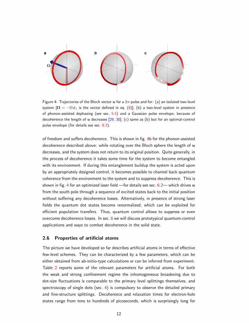
Figure 4: Trajectories of the Bloch vector u for a 2π-pulse and for: (a) an isolated two-level

system [Ω = −Ω e1 is the vector defined in eq. (8)]; (b) a two-level system in presence

of phonon-assisted dephasing (see sec. 5.5) and a Gaussian pulse envelope; because of

decoherence the length of u decreases [29, 30]; (c) same as (b) but for an optimal-control

pulse envelope (for details see sec. 6.2).

of freedom and suffers decoherence. This is shown in fig. 4b for the phonon-assisted

decoherence described above: while rotating over the Bloch sphere the length of u

decreases, and the system does not return to its original position. Quite generally, in

the process of decoherence it takes some time for the system to become entangled

with its environment. If during this entanglement buildup the system is acted upon

by an appropriately designed control, it becomes possible to channel back quantum

coherence from the environment to the system and to suppress decoherence. This is

shown in fig. 4 for an optimized laser field —for details see sec. 6.2— which drives u

from the south pole through a sequence of excited states back to the initial position

without suffering any decoherence losses. Alternatively, in presence of strong laser

fields the quantum dot states become renormalized, which can be exploited for

efficient population transfers. Thus, quantum control allows to suppress or even

overcome decoherence losses. In sec. 6 we will discuss prototypical quantum-control

applications and ways to combat decoherence in the solid state.

2.6 Properties of artificial atoms

The picture we have developed so far describes artificial atoms in terms of effective

few-level schemes. They can be characterized by a few parameters, which can be

either obtained from ab-initio-type calculations or can be inferred from experiment.

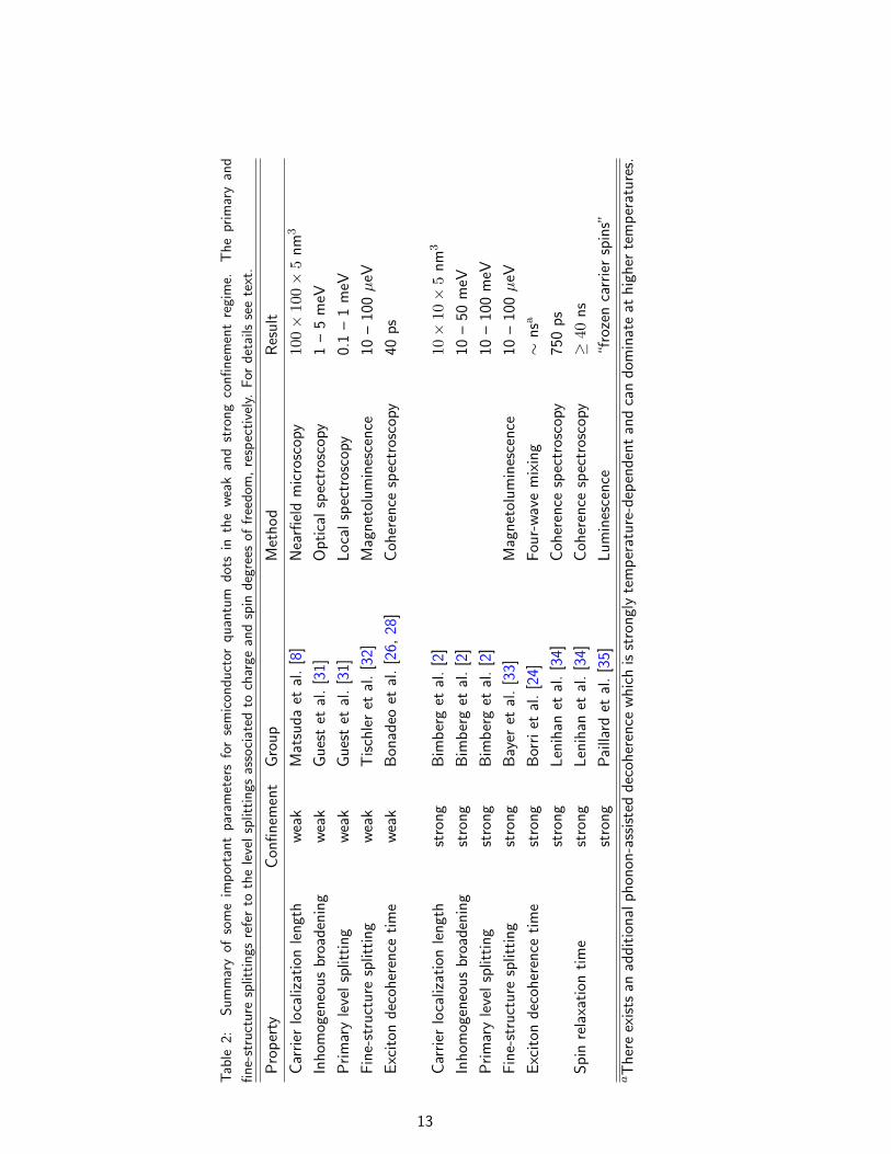
Table 2 reports some of the relevant parameters for artificial atoms. For both

the weak and strong confinement regime the inhomogeneous broadening due to

dot-size fluctuations is comparable to the primary level splittings themselves, and

spectroscopy of single dots (sec. 4) is compulsory to observe the detailed primary

and fine-structure splittings. Decoherence and relaxation times for electron-hole

states range from tens to hundreds of picoseconds, which is surprisingly long for

12

Tab

le2:

Sum

mar

yof

som

eim

por

tant

par

amet

ers

for

sem

icon

duct

orquan

tum

dot

sin

the

wea

kan

dst

rong

confinem

ent

regi

me.

The

prim

ary

and

fine-

stru

cture

split

tings

refe

rto

the

leve

lsp

littings

asso

ciat

edto

char

gean

dsp

indeg

rees

offree

dom

,re

spec

tive

ly.

For

det

ails

see

text

.

Pro

per

tyCon

finem

ent

Gro

up

Met

hod

Res

ult

Car

rier

loca

lizat

ion

lengt

hwea

kM

atsu

da

etal

.[8

]N

earfi

eld

mic

rosc

opy

100×

100×

5nm

3

Inhom

ogen

eous

broa

den

ing

wea

kG

ues

tet

al.[3

1]O

ptica

lsp

ectr

osco

py1

–5

meV

Prim

ary

leve

lsp

litting

wea

kG

ues

tet

al.[3

1]Loca

lsp

ectr

osco

py0.

1–

1m

eV

Fin

e-st

ruct

ure

split

ting

wea

kT

isch

ler

etal

.[3

2]M

agnet

olum

ines

cence

10–

100µeV

Exc

iton

dec

oher

ence

tim

ewea

kB

onad

eoet

al.[2

6,28

]Coh

eren

cesp

ectr

osco

py40

ps

Car

rier

loca

lizat

ion

lengt

hst

rong

Bim

ber

get

al.[2

]10×

10×

5nm

3

Inhom

ogen

eous

broa

den

ing

stro

ng

Bim

ber

get

al.[2

]10

–50

meV

Prim

ary

leve

lsp

litting

stro

ng

Bim

ber

get

al.[2

]10

–10

0m

eV

Fin

e-st

ruct

ure

split

ting

stro

ng

Bay

eret

al.[3

3]M

agnet

olum

ines

cence

10–

100µeV

Exc

iton

dec

oher

ence

tim

est

rong

Bor

riet

al.[2

4]Fou

r-wav

em

ixin

g∼

nsa

stro

ng

Len

ihan

etal

.[3

4]Coh

eren

cesp

ectr

osco

py75

0ps

Spin

rela

xation

tim

est

rong

Len

ihan

etal

.[3

4]Coh

eren

cesp

ectr

osco

py≥

40ns

stro

ng

Pai

llard

etal

.[3

5]Lum

ines

cence

“fro

zen

carr

ier

spin

s”aT

her

eex

ists

anad

ditio

nal

phon

on-a

ssiste

ddec

oher

ence

whic

his

stro

ngl

yte

mper

ature

-dep

enden

tan

dca

ndom

inat

eat

hig

her

tem

per

ature

s.

13

the solid state. This is because of the atomic-like density of states, and the result-

ing inhibition of mutual carrier scatterings and the strong suppression of phonon

scatterings. Yet, when it comes to more sophisticated quantum-control or quantum-

computation applications (secs. 6 and 7) such sub-nanoscecond relaxation and de-

coherence appears to be quite limiting. A possible solution may be provided by spin

excitations, with their long lifetimes because of weak solid-state couplings.

3 Few-particle states

Electron-hole states in semiconductor quantum dots can be described at differ-

ent levels of sophistication, ranging from ab-intio-type approaches over effective

solid-state models to generic few-level schemes. All these approaches have their

respective advantages and disadvantages. For instance, ab-initio-type approaches

provide results that can be quantitatively compared with experiment, but require a

detailed knowledge of the confinement potential which is difficult to obtain in many

cases of interest and often give only little insight into the general physical trends.

On the other hand, few-level schemes grasp all the essential features of certain

electron-hole states in a most simple manner, but the relevant parameters have to

be obtained from either experiment or supplementary calculations. Depending on

the physical problem under consideration we shall thus chose between these dif-

ferent approaches. A description in terms of complementary models is not at all

unique to artificial atoms, but has proven to be a particularly successful concept for

many-electron atoms. These are highly complicated objects whose physical proper-

ties depend on such diverse effects as spin-orbit coupling, exchange interactions, or

Coulomb correlations — and thus make first-principles calculations indispensable

for quantitative predictions. On the other hand, in the understanding of the aufbau

principle of the periodic table it suffices to rely on just a few general rules, such

as Pauli’s principle, Hund’s rules for open-shell atoms, and Coulomb correlation

effects for transition metals. Finally, for quantum optics calculations one usually

invokes generic few-level schemes, e.g. the celebrated Λ- and V-type ones, where

all details of the relevant states are lumped into a few effective parameters. As we

shall see, similar concepts can be successfully extended to semiconductor quantum

dots. In the remainder of this section we shall discuss how this is done.

Throughout we assume that the carrier states in semiconductor quantum dots

are described within a many-body framework such as density functional theory [36],

and can be described by the effective single-particle Schrodinger equation (~ = 1throughout)

14

(−∇

2

2m+ U(r)

)ψ(r) = ε ψ(r) . (9)

In the parentheses on the left-hand side the first term accounts for the kinetic en-

ergy, where m is the free electron mass, and the second one for the atomic-like

potential of the crystal structure. For an ideal periodic solid-state structure the

eigenstates ψnk(r) = unk(r) exp(ikr) are given by the usual Bloch function u,

with n the band index and k the wavevector, and the eigenenergies εnk provide the

semiconductor bandstructure [12, 13, 36]. How are things modified for semicon-

ductor nanostructures? In this paper we shall be concerned with quantum dots with

spatial extensions of typically tens of nanometers in each direction, which consist

of approximately one million atoms. This suggests that the detailed description

of the atomic potential U(r) of eq. (9) is not needed and can be safely replaced

by a more phenomenological description scheme. A particularly simple and suc-

cessful one is provided by the envelope-function approach [12, 13], which assumes

that the single-particle wavefunctions ψ(r) are approximately given by the Bloch

function u of the ideal lattice modulated by an envelope part φ(r) that accounts

for the additional quantum confinement. In the following we consider direct III–V

semiconductors, e.g. GaAs or InAs, whose conduction and valence band extrema

are located at k = 0 and describe the bandstructure near the minima by means of

effective masses me,h for electrons and holes. Then,(− ∇2

2mi+ Ui(r)

)φi

λ(r) = εiλ φiλ(r) (10)

approximately accounts for the electron and hole states in presence of the con-

finement. Here, Ue,h(r) is the effective confinement potential for electrons or

holes, mi is the effective mass of electrons or holes which may depend on position,

e.g. to account for the different semiconductor materials in the confinement of

fig. 1b. In the literature numerous theoretical work —mostly based on the k · p[37, 38, 39, 40] or empirical pseudopotential framework [41, 42, 43]— has been

concerned with more sophisticated calculation schemes for single particle states.

These studies have revealed a number of interesting peculiarities associated to ef-

fects such as piezoelectric fields, strain, or valence-band mixing, but have otherwise

supported the results derived within the more simple-minded envelope-function and

effective-mass description scheme for few-particle states in artificial atoms.

15

3.1 Excitons

3.1.1 Semiconductors of higher dimension

What happens for optical electron-hole excitations which experience in addition to

the quantum confinement also Coulomb interactions? We first recall the description

of a Coulomb-correlated electron-hole pair inside a bulk semiconductor. Within the

envelope-function and effective mass approximations

H = −∑i=e,h

∇2ri

2mi− e2

κs|re − rh|(11)

is the hamiltonian for the interacting electron-hole system, with κs the static di-

electric constant of the bulk semiconductor. In the solution of eq. (11) one usually

introduces the center-of-mass and relative coordinates R = (mere + mhrh)/Mand ρ = re − rh [12], and decomposes H = H+ h into the parts

H = −∇2

R

2M, h = −

∇2ρ

2µ− e2

κs|ρ|, (12)

with M = me +mh and µ = memh/M . Correspondingly, the total wavefunction

can be decomposed into parts Φ(R) and φ(ρ) associated to the center-of-mass

and relative motion, respectively, whose solutions are provided by the Schrodinger

equations

HΦ(R) = EΦ(R), hφ(ρ) = εφ(ρ) . (13)

Here, the first equation describes the motion of a free particle with massM , and the

second one the motion of a particle with mass µ in a Coulomb potential −e2/κs|ρ|.The solutions of the latter equation are those of the hydrogen atom but for the

modified Rydberg energy Es and Bohr radius as of eqs. (2) and (3). Similar

results apply for the lower-dimensional quantum wells and quantum wires provided

that φ(ρ) is replaced by the corresponding two- and one-dimensional wavefunction,

respectively. For instance [12],

φ0(ρ) ∼=4as

exp(−2ρas

)(14)

is the approximate groundstate wavefunction for a two-dimensional quantum well,

whose energy is ε0 = −4Es. For a quantum well of finite width, eq. (14) only

accounts for the in-plane part of the exciton wavefunction. If the quantum well is

sufficiently narrow, the total wavefunction is approximately given by the product

of (14) with the single-particle wavefunctions for electrons and holes along z —i.e.

those of a “particle in the box” [12]—, and the exciton energy is the sum of ε0 with

the single-particle energies for the z-motion of electrons and holes [44, 45, 46].

16

3.1.2 Semiconductor quantum dots

How are the results of the previous section modified in presence of additional quan-

tum confinements Ue(re) and Uh(rh) for electrons and holes? In analogy to eq. (11)

we describe the interacting electron and hole subject to the quantum-dot confine-

ment through the hamiltonian

H =∑i=e,h

(−∇2

ri

2mi+ Ui(ri)

)− e2

κs|re − rh|. (15)

The first term on the right-hand side accounts for the motion of the carriers in

presence of Ui. Because of the additional terms Ui(ri) a separation into center-

of-mass and relative motion is no longer possible. Provided that the potentials

are sufficiently strong, the carrier motion becomes confined in all three spatial

directions. Suppose that L is a characteristic confinement length. Then two limiting

cases can be readily identified in eq. (15): in case of weak confinement where

L as the dynamics of the electron-hole pair is dominated by the Coulomb

attraction, and the confinement potentials Ui(ri) only provide a weak perturbation;

in the opposite case of strong confinement where L as confinement effects

dominate, and the Coulomb part of eq. (15) can be treated perturbatively. In the

following we shall discuss both cases in slightly more detail.

Weak confinement regime. We first consider the weak-confinement regime. A

typical example is provided by monolayer interface fluctuations in the width of a

semiconductor quantum well, as depicted in fig. 1a, where the electron-hole pair

becomes confined within the region of increased quantum-well thickness [4, 5, 6, 8,

31, 48, 49, 50]. If the resulting confinement length L is much larger than the Bohr

radius as, the correlated electron-hole wavefunction factorizes into a center-of-mass

and relative part, where, to a good degree of approximation, the relative part is

given by the wavefunction of the quantum well (“rigid-exciton approximation” [46]).

It then becomes possible to integrate over ρ and to recover an effective Schrodinger

equation for the exciton center-of-mass motion (for details see appendix A)(−∇2

R

2M+ U(R)

)Φx(R) = ExΦx(R) , (16)

where U(R) is a potential obtained through convolution of Ue(re) and Uh(rh) with

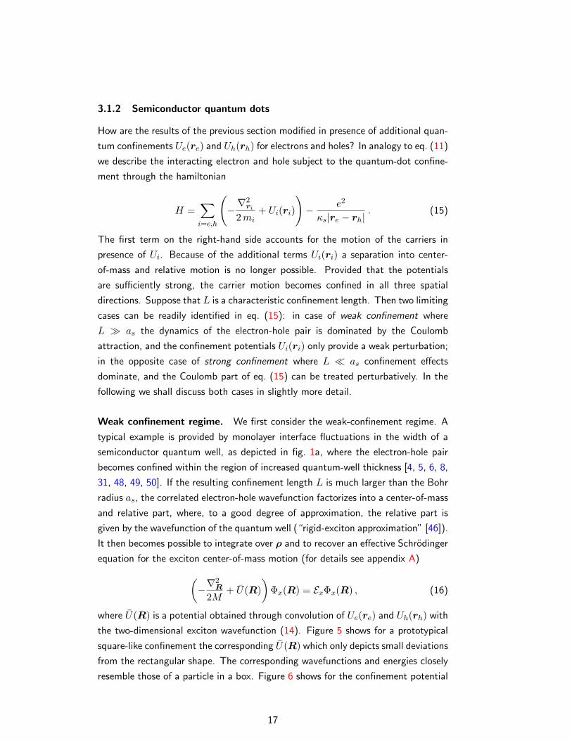
the two-dimensional exciton wavefunction (14). Figure 5 shows for a prototypical

square-like confinement the corresponding U(R) which only depicts small deviations

from the rectangular shape. The corresponding wavefunctions and energies closely

resemble those of a particle in a box. Figure 6 shows for the confinement potential

17

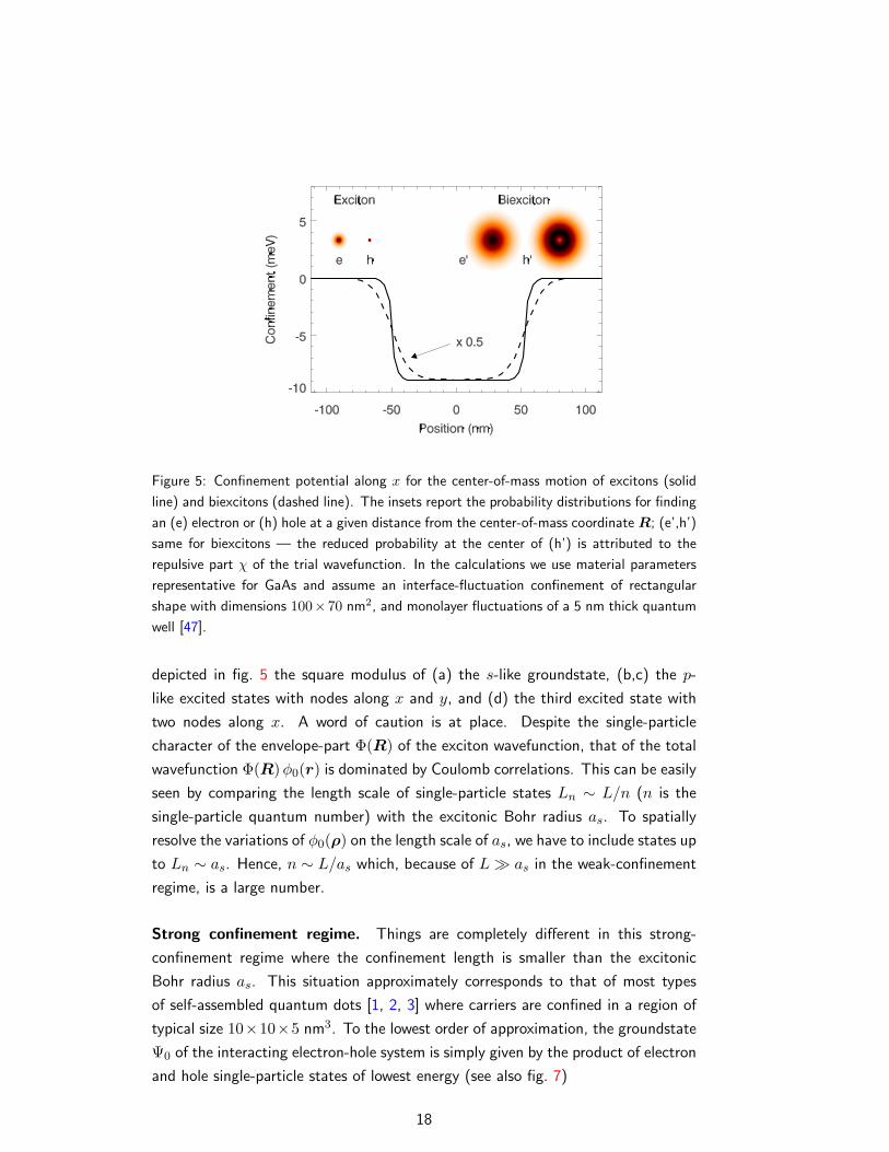
Figure 5: Confinement potential along x for the center-of-mass motion of excitons (solid

line) and biexcitons (dashed line). The insets report the probability distributions for finding

an (e) electron or (h) hole at a given distance from the center-of-mass coordinate R; (e’,h’)

same for biexcitons — the reduced probability at the center of (h’) is attributed to the

repulsive part χ of the trial wavefunction. In the calculations we use material parameters

representative for GaAs and assume an interface-fluctuation confinement of rectangular

shape with dimensions 100×70 nm2, and monolayer fluctuations of a 5 nm thick quantum

well [47].

depicted in fig. 5 the square modulus of (a) the s-like groundstate, (b,c) the p-

like excited states with nodes along x and y, and (d) the third excited state with

two nodes along x. A word of caution is at place. Despite the single-particle

character of the envelope-part Φ(R) of the exciton wavefunction, that of the total

wavefunction Φ(R)φ0(r) is dominated by Coulomb correlations. This can be easily

seen by comparing the length scale of single-particle states Ln ∼ L/n (n is the

single-particle quantum number) with the excitonic Bohr radius as. To spatially

resolve the variations of φ0(ρ) on the length scale of as, we have to include states up

to Ln ∼ as. Hence, n ∼ L/as which, because of L as in the weak-confinement

regime, is a large number.

Strong confinement regime. Things are completely different in this strong-

confinement regime where the confinement length is smaller than the excitonic

Bohr radius as. This situation approximately corresponds to that of most types

of self-assembled quantum dots [1, 2, 3] where carriers are confined in a region of

typical size 10×10×5 nm3. To the lowest order of approximation, the groundstate

Ψ0 of the interacting electron-hole system is simply given by the product of electron

and hole single-particle states of lowest energy (see also fig. 7)

18

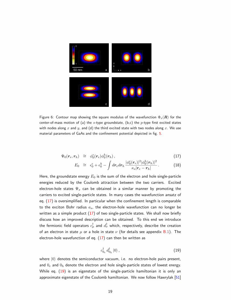
Figure 6: Contour map showing the square modulus of the wavefunction Φx(R) for the

center-of-mass motion of (a) the s-type groundstate, (b,c) the p-type first excited states

with nodes along x and y, and (d) the third excited state with two nodes along x. We use

material parameters of GaAs and the confinement potential depicted in fig. 5.

Ψ0(re, rh) ∼= φe0(re)φh

0(rh) , (17)

E0∼= εe0 + εh0 −

∫dredrh

|φe0(re)|2|φh

0(rh)|2

κs|re − rh|. (18)

Here, the groundstate energy E0 is the sum of the electron and hole single-particle

energies reduced by the Coulomb attraction between the two carriers. Excited

electron-hole states Ψx can be obtained in a similar manner by promoting the

carriers to excited single-particle states. In many cases the wavefunction ansatz of

eq. (17) is oversimplified. In particular when the confinement length is comparable

to the exciton Bohr radius as, the electron-hole wavefunction can no longer be

written as a simple product (17) of two single-particle states. We shall now briefly

discuss how an improved description can be obtained. To this end we introduce

the fermionic field operators c†µ and d†ν which, respectively, describe the creation

of an electron in state µ or a hole in state ν (for details see appendix B.1). The

electron-hole wavefunction of eq. (17) can then be written as

c†0ed†0h

|0〉 , (19)

where |0〉 denotes the semiconductor vacuum, i.e. no electron-hole pairs present,

and 0e and 0h denote the electron and hole single-particle states of lowest energy.

While eq. (19) is an eigenstate of the single-particle hamiltonian it is only an

approximate eigenstate of the Coulomb hamiltonian. We now follow Hawrylak [51]

19

NO

HM

semiconductor bandgap

MH

ON

electrons

holes

Figure 7: Schematic representation of the two possible groundstates of bright excitons in

the strong confinement regime. The solid lines indicate the single-particle states of lowest

energy, and the dotted lines the first excited states. Excited exciton states can be obtained

by promoting the electron or hole to excited single-particle states. The black triangles in

the left and right panel indicate the different spin orientations of the electron and hole, as

discussed in more detail in sec. 3.1.3.

and consider a simplified quantum-dot confinement with cylinder symmetry. The

single-particle states can then be labeled by their angular momentum quantum

numbers, where the groundstate 0 has s-type symmetry and the degenerate first

excited states ±1 have p-type symmetry. Because Coulomb interactions preserve

the total angular momentum [3], the only electron-hole states coupled by Coulomb

interactions to the groundstate are those indicated in fig. 8. We have used that the

angular momentum of the hole is opposite to that of the missing electron. Within

the electron-hole basis |0〉 = |0e, 0h〉 and | ± 1〉 = | ± 1e,±1h〉 the full hamiltonian

matrix is of the form

E0 +

0 Vsp Vsp

Vsp ∆p Vpp

Vsp Vpp ∆p

, (20)

where E0 is the energy (18) of the exciton groundstate, ∆p the detuning of the first

excited state in absence of Coulomb mixing, and Vsp and Vpp describe the Coulomb

couplings between electrons and holes in the s and p shells (see fig. 8). The Coulomb

renormalized eigenstates and energies can then be obtained by diagonalizing the

matrix (20). Results of such configuration-interaction calculations will be presented

in sec. 4 (see appendix B for more details).

3.1.3 Spin structure

Besides the orbital degrees of freedom described by the envelope part of the wave-

function, the atomic part additionally introduces spin degrees of freedom. For III–V

semiconductors an exhaustive description of the band structure near the minima

(at the so-called Γ point) is provided by an eight-band model [12, 52] contain-

20

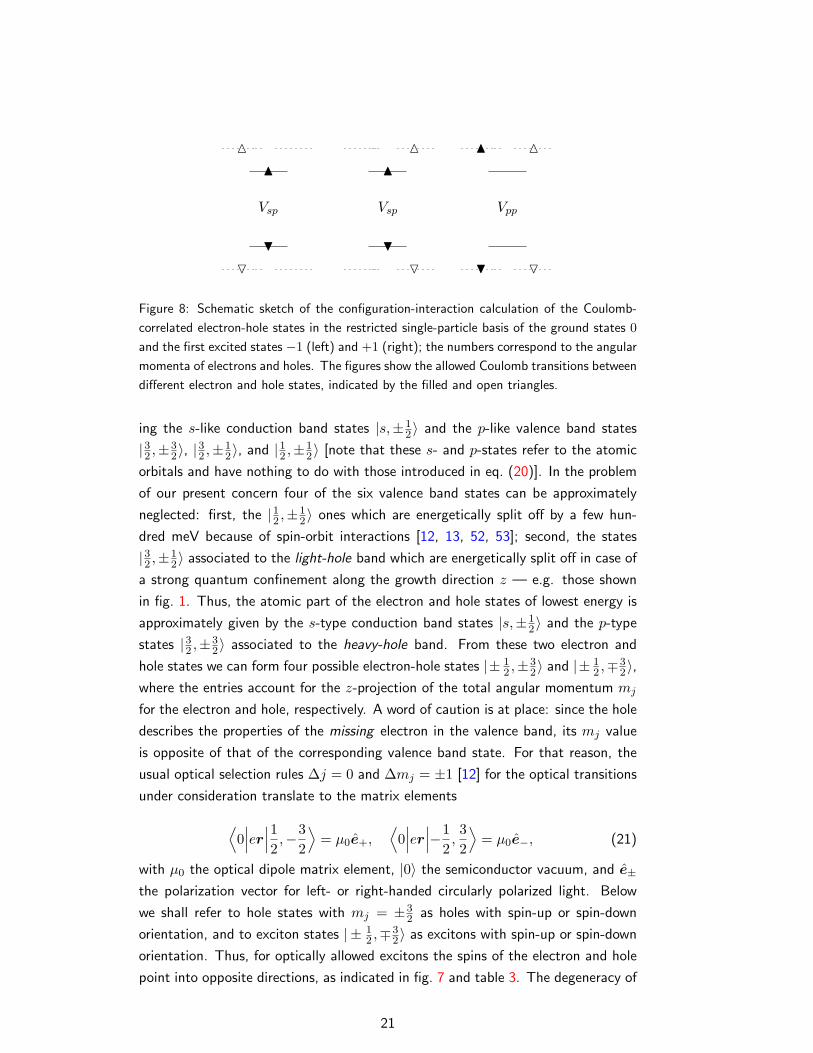
N

M

H

O

Vsp

N

M

H

O

Vsp

N M

H O

Vpp

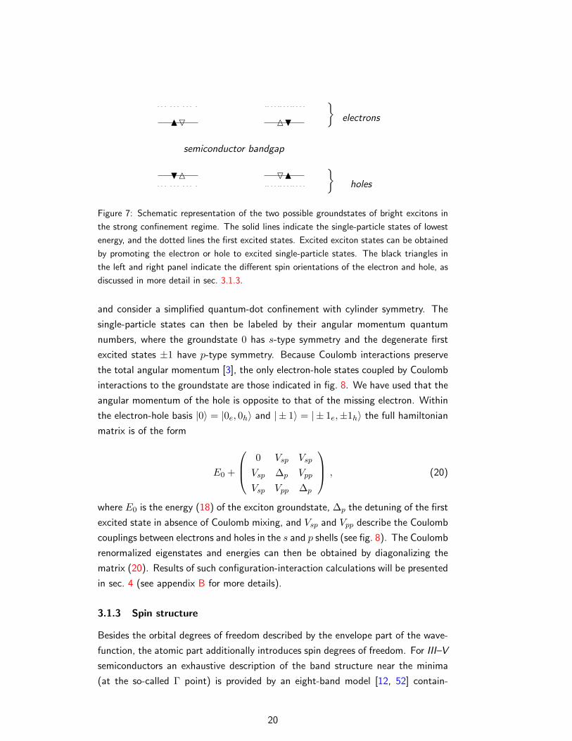
Figure 8: Schematic sketch of the configuration-interaction calculation of the Coulomb-

correlated electron-hole states in the restricted single-particle basis of the ground states 0and the first excited states −1 (left) and +1 (right); the numbers correspond to the angular

momenta of electrons and holes. The figures show the allowed Coulomb transitions between

different electron and hole states, indicated by the filled and open triangles.

ing the s-like conduction band states |s,±12〉 and the p-like valence band states

|32 ,±32〉, |

32 ,±

12〉, and |12 ,±

12〉 [note that these s- and p-states refer to the atomic

orbitals and have nothing to do with those introduced in eq. (20)]. In the problem

of our present concern four of the six valence band states can be approximately

neglected: first, the |12 ,±12〉 ones which are energetically split off by a few hun-

dred meV because of spin-orbit interactions [12, 13, 52, 53]; second, the states

|32 ,±12〉 associated to the light-hole band which are energetically split off in case of

a strong quantum confinement along the growth direction z — e.g. those shown

in fig. 1. Thus, the atomic part of the electron and hole states of lowest energy is

approximately given by the s-type conduction band states |s,±12〉 and the p-type

states |32 ,±32〉 associated to the heavy-hole band. From these two electron and

hole states we can form four possible electron-hole states |± 12 ,±

32〉 and |± 1

2 ,∓32〉,

where the entries account for the z-projection of the total angular momentum mj

for the electron and hole, respectively. A word of caution is at place: since the hole

describes the properties of the missing electron in the valence band, its mj value

is opposite of that of the corresponding valence band state. For that reason, the

usual optical selection rules ∆j = 0 and ∆mj = ±1 [12] for the optical transitions

under consideration translate to the matrix elements

⟨0∣∣∣er∣∣∣1

2,−3

2

⟩= µ0e+,

⟨0∣∣∣er∣∣∣−1

2,32

⟩= µ0e−, (21)

with µ0 the optical dipole matrix element, |0〉 the semiconductor vacuum, and e±

the polarization vector for left- or right-handed circularly polarized light. Below

we shall refer to hole states with mj = ±32 as holes with spin-up or spin-down

orientation, and to exciton states | ± 12 ,∓

32〉 as excitons with spin-up or spin-down

orientation. Thus, for optically allowed excitons the spins of the electron and hole

point into opposite directions, as indicated in fig. 7 and table 3. The degeneracy of

21

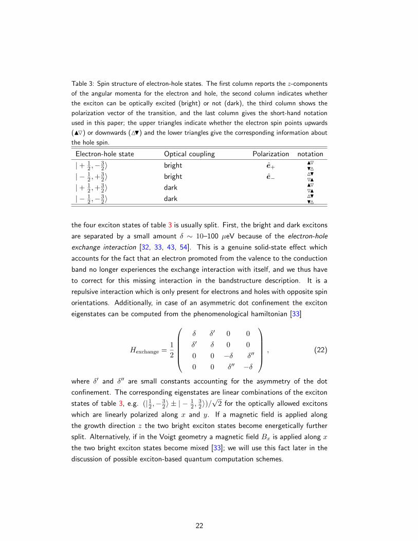
Table 3: Spin structure of electron-hole states. The first column reports the z-components

of the angular momenta for the electron and hole, the second column indicates whether

the exciton can be optically excited (bright) or not (dark), the third column shows the

polarization vector of the transition, and the last column gives the short-hand notation

used in this paper; the upper triangles indicate whether the electron spin points upwards

(NO) or downwards (MH) and the lower triangles give the corresponding information about

the hole spin.

Electron-hole state Optical coupling Polarization notation

|+ 12 ,−

32〉 bright e+

NOHM

| − 12 ,+

32〉 bright e−

MHON

|+ 12 ,+

32〉 dark NO

ON

| − 12 ,−

32〉 dark MH

HM

the four exciton states of table 3 is usually split. First, the bright and dark excitons

are separated by a small amount δ ∼ 10–100 µeV because of the electron-hole

exchange interaction [32, 33, 43, 54]. This is a genuine solid-state effect which

accounts for the fact that an electron promoted from the valence to the conduction

band no longer experiences the exchange interaction with itself, and we thus have

to correct for this missing interaction in the bandstructure description. It is a

repulsive interaction which is only present for electrons and holes with opposite spin

orientations. Additionally, in case of an asymmetric dot confinement the exciton

eigenstates can be computed from the phenomenological hamiltonian [33]

Hexchange =12

δ δ′ 0 0δ′ δ 0 00 0 −δ δ′′

0 0 δ′′ −δ

, (22)

where δ′ and δ′′ are small constants accounting for the asymmetry of the dot

confinement. The corresponding eigenstates are linear combinations of the exciton

states of table 3, e.g. (|12 ,−32〉 ± | −

12 ,

32〉)/

√2 for the optically allowed excitons

which are linearly polarized along x and y. If a magnetic field is applied along

the growth direction z the two bright exciton states become energetically further

split. Alternatively, if in the Voigt geometry a magnetic field Bx is applied along x

the two bright exciton states become mixed [33]; we will use this fact later in the

discussion of possible exciton-based quantum computation schemes.

22

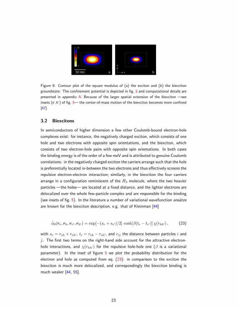
Figure 9: Contour plot of the square modulus of (a) the exciton and (b) the biexciton

groundstate. The confinement potential is depicted in fig. 5 and computational details are

presented in appendix A. Because of the larger spatial extension of the biexciton —see

insets (e’,h’) of fig. 5— the center-of-mass motion of the biexciton becomes more confined

[47].

3.2 Biexcitons

In semiconductors of higher dimension a few other Coulomb-bound electron-hole

complexes exist: for instance, the negatively charged exciton, which consists of one

hole and two electrons with opposite spin orientations, and the biexciton, which

consists of two electron-hole pairs with opposite spin orientations. In both cases

the binding energy is of the order of a few meV and is attributed to genuine Coulomb

correlations: in the negatively charged exciton the carriers arrange such that the hole

is preferentially located in-between the two electrons and thus effectively screens the

repulsive electron-electron interaction; similarly, in the biexciton the four carriers

arrange in a configuration reminiscent of the H2 molecule, where the two heavier

particles —the holes— are located at a fixed distance, and the lighter electrons are

delocalized over the whole few-particle complex and are responsible for the binding

(see insets of fig. 5). In the literature a number of variational wavefunction ansatze

are known for the biexciton description, e.g. that of Kleinman [44]

φ0(re, rh, re′ , rh′) = exp[−(se + se′)/2] cosh[β(te − te′)]χ(rhh′) , (23)

with se = reh + reh′ , te = reh − reh′ , and rij the distance between particles i and

j. The first two terms on the right-hand side account for the attractive electron-

hole interactions, and χ(rhh′) for the repulsive hole-hole one (β is a variational

parameter). In the inset of figure 5 we plot the probability distribution for the

electron and hole as computed from eq. (23): in comparison to the exciton the

biexciton is much more delocalized, and correspondingly the biexciton binding is

much weaker [44, 55].

23

3.2.1 Weak confinement regime

Suppose that the biexciton is subject to an additional quantum confinement, e.g.

induced by the interface fluctuations depicted in fig. 1a. If the characteristic con-

finement length L is larger than the excitonic Bohr radius as and the extension

of the biexciton, one can, in analogy to excitons, introduce a “rigid-biexciton” ap-

proximation: here, the biexciton wavefunction (23) of the ideal quantum well is

modulated by an envelope function which depends on the center-of-mass coordi-

nate of the biexciton. An effective confinement for the biexciton can be obtained

through appropriate convolution of Ui(ri) (for details see appendix A), which is

shown in fig. 5 for a representative interface fluctuation potential. Because of

the larger extension of the biexciton wavefunction, the effective potential exhibits

a larger degree of confinement and correspondingly the biexciton wavefunction of

fig. 9 is more localized. We will return to this point in the discussion of local optical

spectroscopy in sec. 4.4.

3.2.2 Strong confinement regime

In the strong confinement regime the “binding” of few-particle complexes is not

due to Coulomb correlations but to the quantum confinement, whereas Coulomb

interactions only introduce minor energy renormalizations. It thus becomes pos-

sible to confine various few-particle electron-hole complexes which are unstable in

semiconductors of higher dimension. We start our discussion with the few-particle

complex consisting of two electrons and holes. In analogy to higher-dimensional

semiconductors, we shall refer to this complex as a biexciton keeping in mind that

the binding is due to the strong quantum confinement rather than Coulomb cor-

relations. To the lowest order of approximation, the biexciton groundstate Ψ0 in

the strong confinement regime is given by the product of two excitons (17) with

opposite spin orientations

Ψ0(re, rh, re′ , rh′) ∼= Ψ0(re, rh)Ψ0(re′ , rh′) (24)

E0∼= 2E0 + 〈Ψ0|Hee′ +Hhh′ +Heh′ +He′h |Ψ0〉 . (25)

The second term on the right-hand side of eq. (25) accounts for the repulsive and

attractive Coulomb interactions not included in the exciton ground state energy

E0. If electron and hole single-particle states have the same spatial extension,

the repulsive contributions Hee′ and Hhh′ are exactly canceled by the attractive

contributions Heh′ and He′h and the biexciton energy is just twice the exciton

energy, i.e. there is no binding energy for the two neutral excitons. In general, this

description is too simplified. If the electrons and holes arrange in a more favorable

24

∆

0

X

XX

OM

MO

HM

NO

HN

NH

0

E0

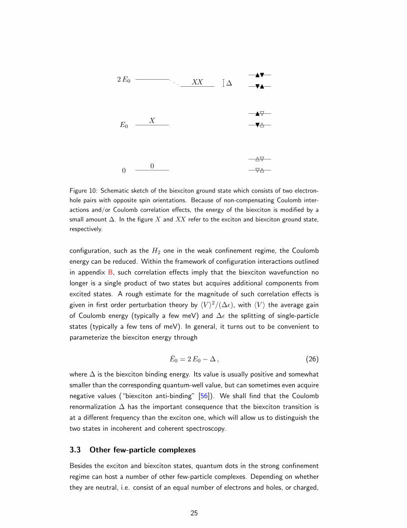
2E0

Figure 10: Schematic sketch of the biexciton ground state which consists of two electron-

hole pairs with opposite spin orientations. Because of non-compensating Coulomb inter-

actions and/or Coulomb correlation effects, the energy of the biexciton is modified by a

small amount ∆. In the figure X and XX refer to the exciton and biexciton ground state,

respectively.

configuration, such as the H2 one in the weak confinement regime, the Coulomb

energy can be reduced. Within the framework of configuration interactions outlined

in appendix B, such correlation effects imply that the biexciton wavefunction no

longer is a single product of two states but acquires additional components from

excited states. A rough estimate for the magnitude of such correlation effects is

given in first order perturbation theory by 〈V 〉2/(∆ε), with 〈V 〉 the average gain

of Coulomb energy (typically a few meV) and ∆ε the splitting of single-particle

states (typically a few tens of meV). In general, it turns out to be convenient to

parameterize the biexciton energy through

E0 = 2E0 −∆ , (26)

where ∆ is the biexciton binding energy. Its value is usually positive and somewhat

smaller than the corresponding quantum-well value, but can sometimes even acquire

negative values (“biexciton anti-binding” [56]). We shall find that the Coulomb

renormalization ∆ has the important consequence that the biexciton transition is

at a different frequency than the exciton one, which will allow us to distinguish the

two states in incoherent and coherent spectroscopy.

3.3 Other few-particle complexes

Besides the exciton and biexciton states, quantum dots in the strong confinement

regime can host a number of other few-particle complexes. Depending on whether

they are neutral, i.e. consist of an equal number of electrons and holes, or charged,

25

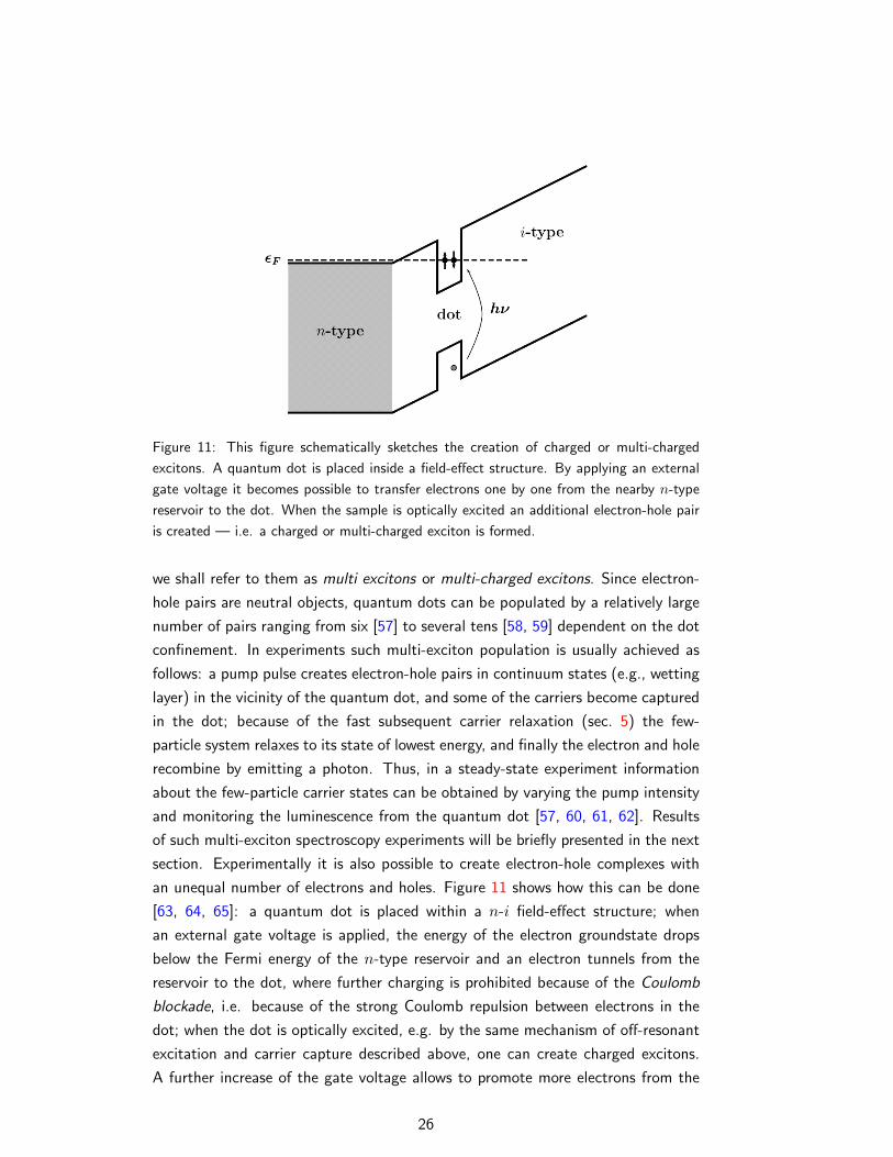
Figure 11: This figure schematically sketches the creation of charged or multi-charged

excitons. A quantum dot is placed inside a field-effect structure. By applying an external

gate voltage it becomes possible to transfer electrons one by one from the nearby n-type

reservoir to the dot. When the sample is optically excited an additional electron-hole pair

is created — i.e. a charged or multi-charged exciton is formed.

we shall refer to them as multi excitons or multi-charged excitons. Since electron-

hole pairs are neutral objects, quantum dots can be populated by a relatively large

number of pairs ranging from six [57] to several tens [58, 59] dependent on the dot

confinement. In experiments such multi-exciton population is usually achieved as

follows: a pump pulse creates electron-hole pairs in continuum states (e.g., wetting

layer) in the vicinity of the quantum dot, and some of the carriers become captured

in the dot; because of the fast subsequent carrier relaxation (sec. 5) the few-

particle system relaxes to its state of lowest energy, and finally the electron and hole

recombine by emitting a photon. Thus, in a steady-state experiment information

about the few-particle carrier states can be obtained by varying the pump intensity

and monitoring the luminescence from the quantum dot [57, 60, 61, 62]. Results

of such multi-exciton spectroscopy experiments will be briefly presented in the next

section. Experimentally it is also possible to create electron-hole complexes with

an unequal number of electrons and holes. Figure 11 shows how this can be done

[63, 64, 65]: a quantum dot is placed within a n-i field-effect structure; when

an external gate voltage is applied, the energy of the electron groundstate drops

below the Fermi energy of the n-type reservoir and an electron tunnels from the

reservoir to the dot, where further charging is prohibited because of the Coulomb

blockade, i.e. because of the strong Coulomb repulsion between electrons in the

dot; when the dot is optically excited, e.g. by the same mechanism of off-resonant

excitation and carrier capture described above, one can create charged excitons.

A further increase of the gate voltage allows to promote more electrons from the

26

reservoir to the dot, and to hereby create multi-charged excitons with up to two

surplus electrons. In Regelman et al. [66] a quantum dot was placed in a n-i-

p structure which allowed to create in the same sample either negatively (more

electrons than holes) or positively (more holes than electrons) charged excitons by

varying the applied gate voltage. A different approach was pursued by Hartmann

et al. [67], where charging was achieved by unintentional background doping and

the mechanism of photo depletion, which allowed to charge quantum dots with up

to five surplus electrons. Luminescence spectra of such multi-charged excitons will

be presented in sec. 4.2.

3.4 Coupled dots

We conclude this section with a brief discussion of coupled quantum dots. In

analogy to artificial atoms, we may refer to coupled dots as artificial molecules.

Coupling is an inherent feature of any high-density quantum dot ensemble, as,

e.g. needed for most optoelectronic applications [2]. On the other hand, it is

essential to the design of (quantum) information devices, for example quantum dot

cellular automata [68] or quantum-dot implementations of quantum computation

(sec. 7). Artificial molecules formed by two or more coupled dots are extremely

interesting also from the fundamental point of view, since the interdot coupling

can be tuned far out of the regimes accessible in natural molecules, and the relative

importance of single-particle tunneling and Coulomb interactions can be varied

in a controlled way. The interacting few-electron states in a double dot were

studied theoretically [69, 70, 71] and experimentally by tunneling and capacitance

experiments [72, 73, 74, 75, 76, 77, 78, 79], and correlations were found to induce

coherence effects and novel ground-state phases depending on the interdot coupling

regime. For self-organized dots stacking was demonstrated [80], and the exciton

splitting in a single artificial molecule was observed and explained in terms of single-

particle level filling of delocalized bonding and anti-bonding electron and hole states

[81, 82, 83]. When a few photoexcited particles are present, Coulomb coupling

between electrons and holes adds to the homopolar electron-electron and hole-hole

couplings. In addition, single-particle tunneling and kinetic energies are affected by

the different spatial extension of electrons and holes, and the correlated ground and

excited states are governed by the competition of these effects [69, 84, 85, 86]. A

particularly simple parameterization of single-exciton and biexciton states in coupled

dots is given by the Hubbard-type hamiltonian [87]

H = E0

∑σ

(nLσ + nRσ)− t∑

σ

(b†LσbRσ + b†RσbLσ

)−∆

∑`=L,R

n`↑n`↓ , (27)

27

with b†`σ the creation operator for excitons with spin orientation σ = ± in the

right or left dot, n`σ = b†`σb`σ the exciton number operator, t the tunneling matrix

element, and ∆ the biexciton binding. Indeed, the hamiltonian (27) accounts

properly for the formation of bonding and anti-bonding exciton states, and the fact

that in a biexciton state the two electron-hole pairs preferentially stay together to

benefit from the biexciton binding ∆ [69, 84]. We will return to coupled dots in

the discussion of quantum control (sec. 6) and quantum computation (sec. 7).

4 Optical spectroscopy

In the last section we have discussed the properties of electron-hole states in semi-

conductor quantum dots. We shall now show how these states couple to the light

and can be probed optically. Our starting point is given by eq. (9) which describes

the propagation of one electron subject to the additional quantum confinement

U . Quite generally, the light field is described by the vector potential A and the

light-matter coupling is obtained by replacing the momentum operator p = −i∇with p − (q/c)A [13, 15], where q = −e is the charge of the electron and c the

speed of light. The light-matter coupling then follows from(p+ e

c A)2

2m+ U(r) = H0 +

e

mcAp+

e2

2mc2A2 , (28)

where we have used the Coulomb gauge ∇A = 0 [88] to arrive at the Ap term. In

many cases of interest the spatial dependence of A can be neglected on the length

scale of the quantum states, i.e. in the far-field limit —recall that the length scales

of light and matter are given by microns and nanometers, respectively—, and we

can perform a gauge transformation to replace the Ap term by the well-known

dipole coupling [15]

Hop =e

mcAp ∼= er E . (29)

The relation between the vector potential and the electric field is given by E =(1/c)∂A/∂t. In this far-field limit we can also safely neglect the A2 term. This is

because the matrix elements 〈0| ± 12 ,∓

32〉 between the atomic states introduced in

sec. 3.1.3 vanish owing to the orthogonality of conduction and valence band states.

Equation (29) is suited for both classical and quantum light fields. In the first case

E is treated as a c-number, in the latter case the electric field of photons reads

[15, 22, 89, 90]

E ∼= i∑kλ

(2πωk

κs

) 12 (ekλ akλ − e∗kλ a

†kλ

). (30)

28

Here, k and λ are the photon wavevector and polarization, respectively, ωk = ck/ns

is the light frequency, ns =√κs the semiconductor refractive index, ekλ the photon

polarization vector, and akλ denotes the usual bosonic field operator. The free

photon field is described by the hamiltonian Hγ0 =

∑kλ ωk a

†kλakλ.

Optical dipole moments. Optical selection rules were already introduced in

sec. 3.1.3 where we showed that light with appropriate polarization λ —i.e. for

light propagation along z either circular polarization for symmetric dots or lin-

ear polarization for asymmetric ones— can induce electron-hole transitions. We

shall now show how things are modified when additionally the envelope part of the

carrier wavefunctions is considered. In second quantization (see appendix B) the

light-matter coupling of eq. (29) reads

Hop∼=∑

λ

∫dr(µ0eλψ

hλ(r)ψe

λ(r) + h.c.)

E , (31)

where λ is the polarization mode orthogonal to λ. Because of the envelope-function

approximation the dipole operator er has been completely absorbed in the bulk

moment µ0 [12, 13]. The first term in parentheses of eq. (31) accounts for the

destruction of an electron-hole pair, and the second one for its creation. Similarly,

in an all-electron picture the two terms can be described as the transfer of an

electron from the conduction to the valence band or vice versa. This single-particle

nature of optical excitations translates to the requirement that electron and hole

are destroyed or created at the same position r. Equation (31) usually comes

together with the so-called rotating-wave approximation [12, 15]. Consider the

light-matter coupling (31) in the interaction picture according to the hamiltonian

of the unperturbed system: the first term, which accounts for the annihilation of an

electron-hole pair, then approximately oscillates with e−iω0t and the second term

with eiω0t, where ω0 is a frequency of the order of the semiconductor band gap.

Importantly, ω0 sets the largest energy scale (eV) of the problem whereas all exciton

or few-particle level splittings are substantially smaller. If we accordingly separate

E into terms oscillating with approximately e±iω0t, we encounter in the light-matter

coupling of eq. (31) two possible combinations of exponentials: first, those with

e±i(ω0−ω0)t which have a slow time dependence and have to be retained; second,

those with e±i(ω0+ω0)t which oscillate with twice the frequency of the band gap. In

the spirit of the random-phase approximation, the latter off-resonant terms do not

induce transitions and can thus be neglected. Then, the light-matter coupling of

eq. (31) becomes

Hop∼=

12

(P E(−) + P† E(+)

), (32)

29

where E(±) ∝ e∓iω0t solely evolves with positive or negative frequency compo-

nents, and the complex conjugate of E(−) is given by E(+) [22]. In eq. (32) P =∑λ µ0eλ

∫dr ψh

λ(r)ψe

λ(r) is the usual interband polarization operator [12, 91].

Let us finally briefly discuss the optical dipole elements for excitonic and biexci-

tonic transitions. Within the framework of second quantization the exciton and

biexction states |xλ〉 and |b〉 can be expressed as

|xλ〉 =∫dτ Ψx(re, rh)ψe †

λ (re)ψh †λ

(rh) |0〉 (33)

|b〉 =∫dτ Ψb(re, rh, r

′e, r

′h)ψe †

λ (re)ψh †λ

(rh)ψe †λ

(r′e)ψh †λ (r′h) |0〉 , (34)

with dτ and dτ denoting the phase space for excitons and biexcitons, respectively.

In eq. (33) the exciton state consists of one electron and hole with opposite spin

orientations, and in eq. (34) the biexciton of two electron-hole pairs with opposite

spin orientations. From the light-matter coupling (31) we then find for the optical

dipole elements

〈0|P |xλ〉 =M0xeλ = µ0 eλ

∫drΨx(r, r) (35)

〈xλ|P |b〉 =Mxb eλ = µ0 eλ

∫drdredrh Ψ∗

x(re, rh)Ψb(r, r, re, rh) . (36)

In eq. (35) the dipole moment is given by the spatial average of the exciton wave-

function Ψx(r, r) where the electron and hole are at the same position r. Similarly,

in eq. (36) the dipole moment is given by the overlap of exciton and biexciton wave-

functions subject to the condition that the electron with spin λ and the hole with

spin λ are at the same position r, whereas the other electron and hole remain at

the same position. In appendix A.3 we show that in the weak confinement regime

the oscillator strength for optical transitions scales with the confinement length L

according to |M0x|2 ∝ L2, i.e. it is proportional to the confinement area. For that

reason excitons in the weak-confinement regime couple much stronger to the light

than those in the strong confinement regime, which makes them ideal candidates

for various kinds of optical coherence experiments [8, 26, 28, 90, 92, 93, 94, 95].

Fluctuation-dissipation theorem. We next discuss how to compute optical spec-

tra in linear response. As a preliminary task we consider the general situation where

a generic quantum system is coupled to an external perturbation X(t), e.g. an ex-

citing laser light, via the system operator A through AX(t) [96]. Let 〈B〉 be the

expectation value of the operator B in the perturbed system and 〈B〉0 that in the

unperturbed one. In linear-response theory the change 〈∆B〉 = 〈B〉 − 〈B〉0 is as-

sumed to be linear in the perturbation X(t) — an approximation valid under quite

30

broad conditions provided that the external perturbation is sufficiently weak. We

can then derive within lowest-order time-dependent perturbation theory the famous

fluctuation-dissipation theorem [96]

〈∆B(0)〉 = i

∫ 0

−∞dt′ 〈[A(t′), B(0)]〉0X(t′) , (37)

where operators A and B are given in the interaction picture according to the

unperturbed system hamiltonian H0. In eq. (37) we have assumed that the external

perturbation has been turned on at sufficiently early times such that the system

has reached equilibrium. The important feature of eq. (37) is that it relates the

expectation value of B in the perturbed system to the correlation [A,B] —or

equivalently to the fluctuation [∆A,∆B] because commutators with c-numbers

always vanish— of the unperturbed system. Usually, the expression on the right-

hand side of eq. (37) is much easier to compute than that on the left-hand side.

We will next show how the fluctuation-dissipation theorem (37) can be used for the

calculation of linear optical absorption and luminescence.

4.1 Optical absorption

Absorption describes the process where energy is transferred from the light field to

the quantum dot, i.e. light becomes absorbed. Absorption is proportional to the

loss of energy of the light field, or equivalently to the gain of energy of the system

α(ω) ∝ d

dt〈H0 +Hop〉 =

⟨∂Hop

∂t

⟩. (38)

Consider a mono-frequent excitation E0eλ cosωt, where E0 is the amplitude of the

light field. Inserting this expression into eq. (38) gives after some straightforward

calculation α(ω) ∝ −ωE0=m(eiωt〈e∗λP〉

). From the fluctuation-dissipation theo-

rem we then find

αλ(ω) ∝ =m(i

∫ 0

−∞dt′⟨[e∗λP(0), eλP†(t′)

]⟩0e−iωt′

), (39)

i.e. optical absorption is proportional to the spectrum of interband polarization

fluctuations. We emphasize that this is a very general and important result that

holds true for systems at finite temperatures, and is used for ab-initio type calcu-

lations of optically excited semiconductors [97]. We next show how to evaluate

eq. (39). Suppose that the quantum dot is initially in its groundstate. Then only

the term 〈0|P(0)P†(t′)|0〉 contributes in eq. (39) because no electron-hole pair

can be destroyed in the vacuum, i.e. P |0〉 = 0. Through P†(t′)|0〉 an electron-hole

pair is created in the quantum dot which propagates in presence of the quantum

confinement and the Coulomb attraction between the electron and hole. Thus, the

31

propagation of the interband polarization can be computed by use of the exciton

eigenstates |x〉 through 〈x|P†(t′)|0〉 = eiExt 〈x|P†|0〉. Inserting the complete set

of exciton eigenstates in eq. (39) gives

α(ω) ∝ =m

(i∑xλ

∫ 0

−∞dt′ |M0xλ

|2 e−i(ω−Exλ)t′

). (40)

To evaluate the integral in eq. (40) we have to assume that the exciton energy has

a small imaginary part Ex − iγ associated to the finite exciton lifetime because of

environment couplings (sec. 5). Then,∫ 0−∞ dt′e−i(ω−Ex+iγ) = i/(ω−Ex + iγ) and

we obtain for the optical absorption the final result

α(ω) ∝∑xλ

|M0xλ|2 δγ(ω − Exλ

) . (41)

Here δγ(ω) = γ/(ω2 + γ2) is a Lorentzian which in the limit γ → 0 gives Dirac’s

delta function. According to eq. (41) the absorption spectrum of a single quantum

dot is given by a comb of delta-like peaks at the energies of the exciton states,

whose intensities —sometimes referred to as the oscillator strengths— are given by

the square modulus of the dipole moments (35).

4.1.1 Weak confinement

In the weak confinement regime the absorption spectrum is given by

α(ω) ∝∑

x

∣∣∣∣∫ dRΦx(R)∣∣∣∣2 δγ(ω − Ex) , (42)

where Φx(R) is the center-of-mass wavefunction introduced in sec. 3.1. Let us con-

sider the somewhat simplified example of a rectangular confinement with infinite

barriers whose solutions are Φ(X,Y ) = 2/(L1L2)12 sin(n1πX/L1) sin(n2π Y/L2).

Here X and Y are the center-of-mass coordinates along x and y, L1 and L2

are the confinement lengths in x- and y-direction, and n1 and n2 the corre-

sponding quantum numbers. The energy associated to this wavefunction is E =π2/(2M) [(n1/L1)2 + (n2/L2)2]. Inserting these expressions into eq. (42) shows

that the oscillator strength is zero when n1 or n2 is an even number, and propor-

tional to L1L2/(n1n2) otherwise. Figure 12 shows absorption spectra computed

within this framework for (a) an inhomogeneously broadened ensemble of quantum

dots and (b) a single dot. The first situation corresponds to typical optical experi-

ments performed on ensembles of quantum dots. Single dots can be measured by

different types of local spectroscopy such as submicron apertures [4, 31, 48, 62, 98],

solid immersion microscopy [50, 99], or scanning near-field microscopy [8, 94, 100].

Note that such single-dot spectroscopy is indispensable for the observation of the

32

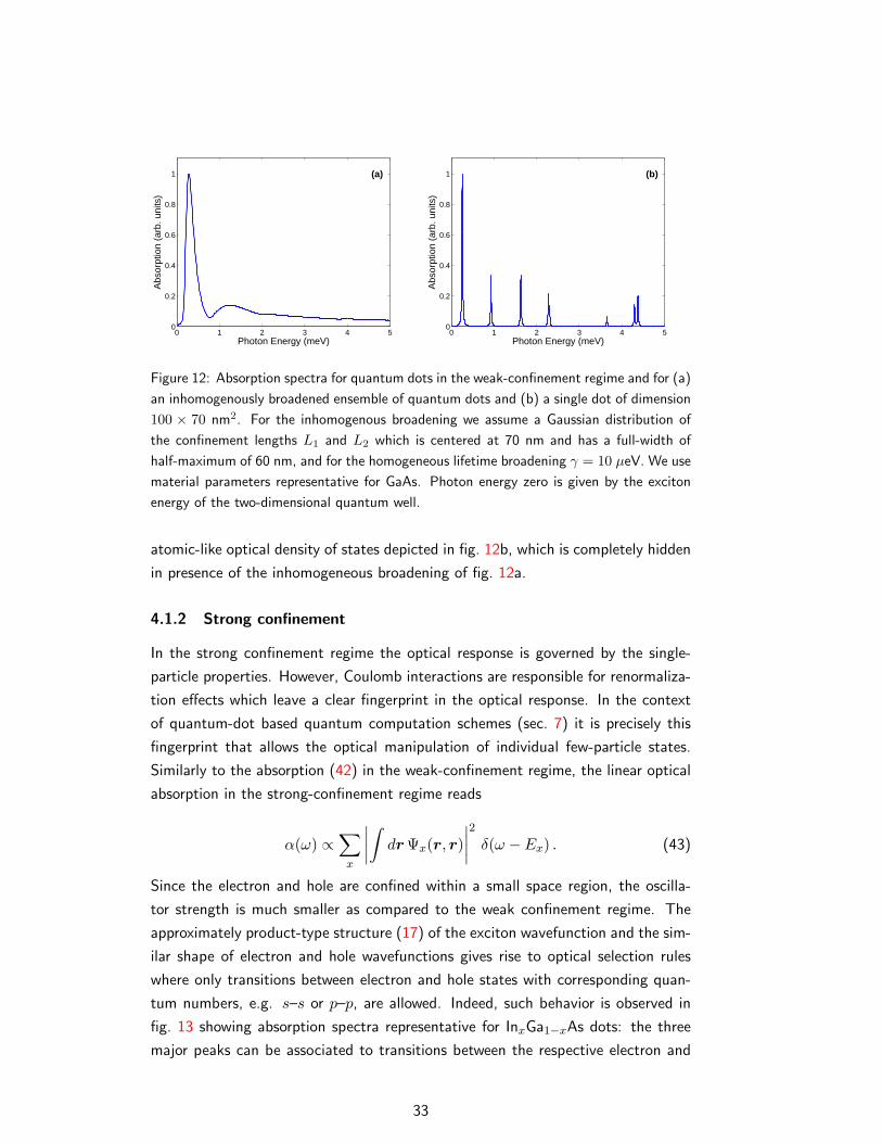
0 1 2 3 4 50

0.2

0.4

0.6

0.8

1 (a)

Photon Energy (meV)

Abs

orpt

ion

(arb

. uni

ts)

0 1 2 3 4 50

0.2

0.4

0.6

0.8

1 (b)

Photon Energy (meV)

Abs

orpt

ion

(arb

. uni

ts)

Figure 12: Absorption spectra for quantum dots in the weak-confinement regime and for (a)

an inhomogenously broadened ensemble of quantum dots and (b) a single dot of dimension

100 × 70 nm2. For the inhomogenous broadening we assume a Gaussian distribution of

the confinement lengths L1 and L2 which is centered at 70 nm and has a full-width of

half-maximum of 60 nm, and for the homogeneous lifetime broadening γ = 10 µeV. We use

material parameters representative for GaAs. Photon energy zero is given by the exciton

energy of the two-dimensional quantum well.

atomic-like optical density of states depicted in fig. 12b, which is completely hidden

in presence of the inhomogeneous broadening of fig. 12a.

4.1.2 Strong confinement

In the strong confinement regime the optical response is governed by the single-

particle properties. However, Coulomb interactions are responsible for renormaliza-

tion effects which leave a clear fingerprint in the optical response. In the context

of quantum-dot based quantum computation schemes (sec. 7) it is precisely this

fingerprint that allows the optical manipulation of individual few-particle states.

Similarly to the absorption (42) in the weak-confinement regime, the linear optical

absorption in the strong-confinement regime reads

α(ω) ∝∑

x

∣∣∣∣∫ drΨx(r, r)∣∣∣∣2 δ(ω − Ex) . (43)

Since the electron and hole are confined within a small space region, the oscilla-

tor strength is much smaller as compared to the weak confinement regime. The

approximately product-type structure (17) of the exciton wavefunction and the sim-

ilar shape of electron and hole wavefunctions gives rise to optical selection rules

where only transitions between electron and hole states with corresponding quan-

tum numbers, e.g. s–s or p–p, are allowed. Indeed, such behavior is observed in

fig. 13 showing absorption spectra representative for InxGa1−xAs dots: the three

major peaks can be associated to transitions between the respective electron and

33

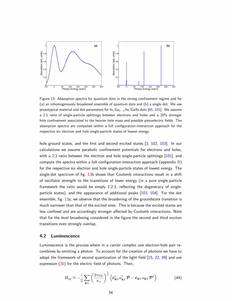
−50 0 50 100 150 200 250 3000

0.2

0.4

0.6

0.8

1 (a)

Photon Energy (meV)

Abs

orpt

ion

(arb

. uni

ts)

−50 0 50 100 150 200 250 3000

0.2

0.4

0.6

0.8

1 (b)

Photon Energy (meV)

Abs

orpt

ion

(arb

. uni

ts)

Figure 13: Absorption spectra for quantum dots in the strong confinement regime and for

(a) an inhomogenously broadened ensemble of quantum dots and (b) a single dot. We use

prototypical material and dot parameters for InxGa1−xAs/GaAs dots [65, 101]. We assume

a 2:1 ratio of single-particle splittings between electrons and holes and a 20% stronger

hole confinement associated to the heavier hole mass and possible piezoelectric fields. The

absorption spectra are computed within a full configuration-interaction approach for the

respective six electron and hole single-particle states of lowest energy.

hole ground states, and the first and second excited states [3, 102, 103]. In our

calculations we assume parabolic confinement potentials for electrons and holes,

with a 2:1 ratio between the electron and hole single-particle splittings [101], and

compute the spectra within a full configuration-interaction approach (appendix B)

for the respective six electron and hole single-particle states of lowest energy. The

single-dot spectrum of fig. 13b shows that Coulomb interactions result in a shift

of oscillator strength to the transitions of lower energy (in a pure single-particle

framework the ratio would be simply 1:2:3, reflecting the degeneracy of single-

particle states), and the appearance of additional peaks [103, 104]. For the dot

ensemble, fig. 13a, we observe that the broadening of the groundstate transition is

much narrower than that of the excited ones. This is because the excited states are

less confined and are accordingly stronger affected by Coulomb interactions. Note

that for the level broadening considered in the figure the second and third exciton

transitions even strongly overlap.

4.2 Luminescence

Luminescence is the process where in a carrier complex one electron-hole pair re-

combines by emitting a photon. To account for the creation of photons we have to

adopt the framework of second quantization of the light field [15, 22, 89] and use

expression (30) for the electric field of photons. Then,

Hop∼= − i

2

∑kλ

(2πωk

κs

) 12 (e∗kλ a

†kλ P − ekλ akλ P†

)(44)

34

is the hamilton operator which describes the photon-matter coupling within the

envelope-function and rotating-wave approximations. The first term on the right-

hand side describes the destruction of an electron-hole pair through photon emis-

sion, and the second one the reversed process. We shall now show how to compute

from eq. (44) the luminescence spectrum L(ω). It is proportional to the increase

in the number of photons 〈a†kλakλ〉 emitted at a given energy ω. With this approx-

imation we obtain

L(ω) ∝ d

dt

(∑kλ

⟨a†kλakλ

⟩δ(ω − ωkλ)

). (45)

We next use Heisenberg’s equation of motion O = −i[O,H], with O an arbi-

trary time-independent operator, and 〈[a†kλakλ,H]〉 = 2i=m〈a†kλ[akλ,Hop]〉. By

computing the commutator with Hop, eq. (44), we obtain

L(ω) ∝∑kλ

(2πωk

κs

) 12

=m⟨a†kλ e

∗kλP

⟩δ(ω − ωkλ) . (46)

The expression 〈a†P〉 is known as the photon-assisted density matrix [27, 105].

It describes the correlations between the photon and the electron-hole excitations

in the quantum dot. Again, we can use the fluctuation-dissipation theorem (37)

to compute eq. (46) and to provide a relation between the photon-assisted density

matrix and the correlation function 〈[a†kλ(0)P(0), ak′λ′(t)P†(t)]〉. The calculation

can be considerably simplified if we make the reasonable assumption that before

photon emission no other photons are present. Then, only 〈ak′λ′a†kλ〉 = δkk′δλλ′

does not vanish. It is diagonal in k and λ because the only photon that can be

destroyed by the annihilation operator a is the one created by a†. Thus,

L(ω) ∝ π∑kλ

2πωkµ20

κs=m

(i

∫ 0

−∞dt′⟨ekλP†(t′) e∗kλP(0)

⟩eiωt

)δ(ω − ωkλ) .

(47)

Suppose that the system is initially in the eigenstate |i〉 of the unperturbed system

which has energy Ei. We next insert a complete set of eigenstates∑

f |f〉〈f | in

the above equation (note that because the interband polarization operator P can

only remove one electron-hole pair the states f and i differ by one electron and

hole), and assume that only photons propagating along z with polarization λ are

detected. Then,

L(ω) ∝∑

f

|〈f |e∗λP |i〉|2 δγ(Ef + ω − Ei) (48)

35

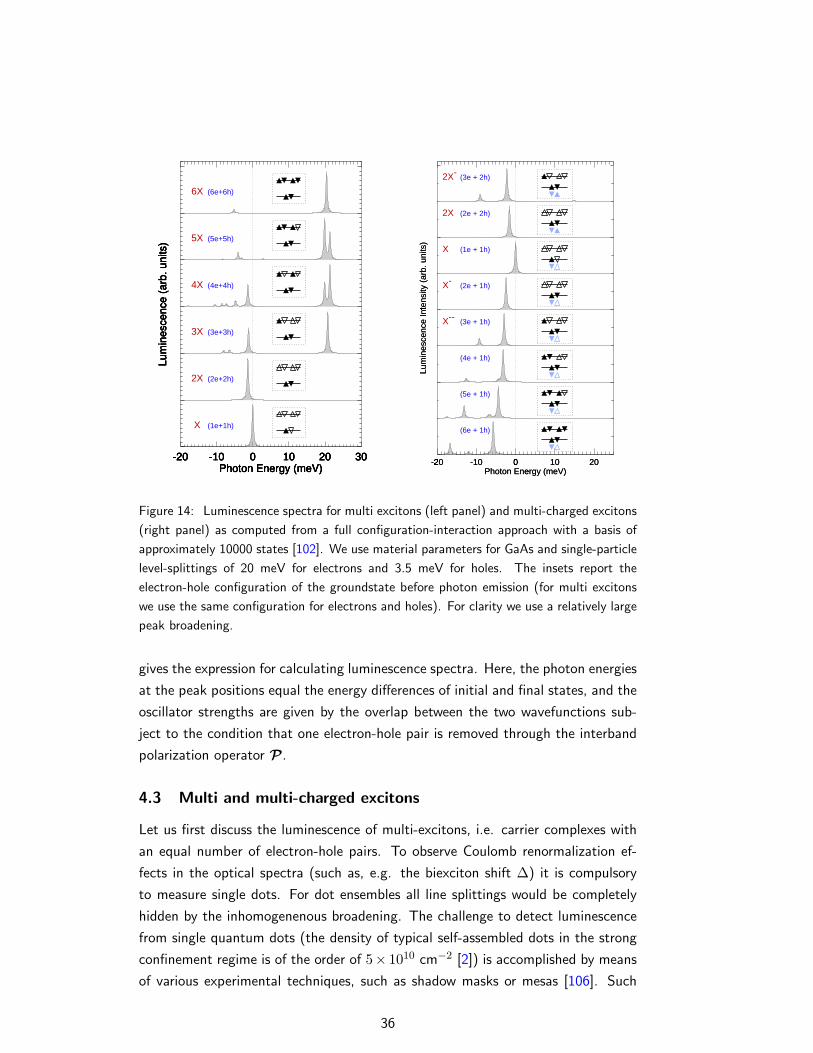
-20 -10 0 10 20 30Photon Energy (meV)

Lu

min

esce

nce

(arb

. uni

ts)

6X (6e+6h)

5X (5e+5h)

4X (4e+4h)

3X (3e+3h)

2X (2e+2h)

X (1e+1h)

-20 -10 0 10 20 30Photon Energy (meV)

Lu

min

esce

nce

(arb

. uni

ts)

-20

-10 0 10 20Photon Energy (meV)

Lum

ines

cenc

e In

tens

ity (

arb.

uni

ts)

2X-(3e + 2h)

2X (2e + 2h)

X (1e + 1h)

X-(2e + 1h)

X--(3e + 1h)

(4e + 1h)

(5e + 1h)

(6e + 1h)

-20

-10 0 10 20Photon Energy (meV)

Lum

ines

cenc

e In

tens

ity (

arb.

uni

ts)

Figure 14: Luminescence spectra for multi excitons (left panel) and multi-charged excitons

(right panel) as computed from a full configuration-interaction approach with a basis of

approximately 10000 states [102]. We use material parameters for GaAs and single-particle

level-splittings of 20 meV for electrons and 3.5 meV for holes. The insets report the

electron-hole configuration of the groundstate before photon emission (for multi excitons

we use the same configuration for electrons and holes). For clarity we use a relatively large

peak broadening.

gives the expression for calculating luminescence spectra. Here, the photon energies

at the peak positions equal the energy differences of initial and final states, and the

oscillator strengths are given by the overlap between the two wavefunctions sub-

ject to the condition that one electron-hole pair is removed through the interband

polarization operator P .

4.3 Multi and multi-charged excitons

Let us first discuss the luminescence of multi-excitons, i.e. carrier complexes with

an equal number of electron-hole pairs. To observe Coulomb renormalization ef-

fects in the optical spectra (such as, e.g. the biexciton shift ∆) it is compulsory

to measure single dots. For dot ensembles all line splittings would be completely

hidden by the inhomogenenous broadening. The challenge to detect luminescence

from single quantum dots (the density of typical self-assembled dots in the strong

confinement regime is of the order of 5× 1010 cm−2 [2]) is accomplished by means

of various experimental techniques, such as shadow masks or mesas [106]. Such

36

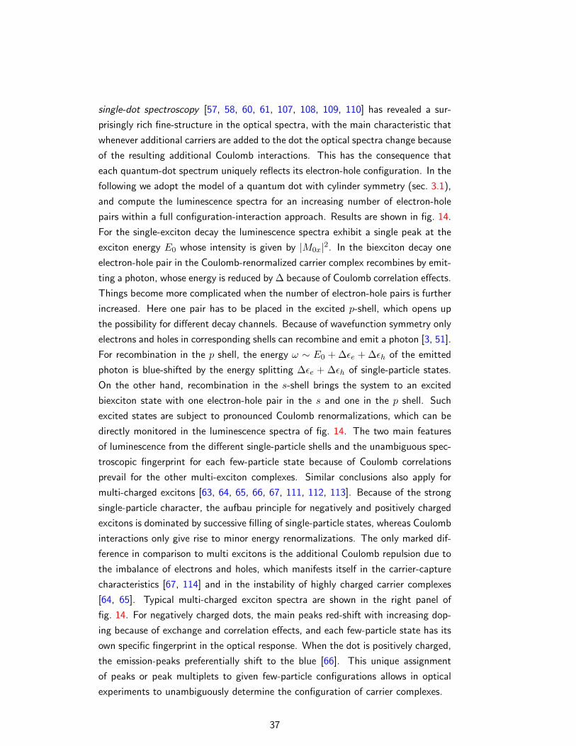
single-dot spectroscopy [57, 58, 60, 61, 107, 108, 109, 110] has revealed a sur-

prisingly rich fine-structure in the optical spectra, with the main characteristic that

whenever additional carriers are added to the dot the optical spectra change because

of the resulting additional Coulomb interactions. This has the consequence that

each quantum-dot spectrum uniquely reflects its electron-hole configuration. In the

following we adopt the model of a quantum dot with cylinder symmetry (sec. 3.1),

and compute the luminescence spectra for an increasing number of electron-hole

pairs within a full configuration-interaction approach. Results are shown in fig. 14.

For the single-exciton decay the luminescence spectra exhibit a single peak at the

exciton energy E0 whose intensity is given by |M0x|2. In the biexciton decay one

electron-hole pair in the Coulomb-renormalized carrier complex recombines by emit-

ting a photon, whose energy is reduced by ∆ because of Coulomb correlation effects.

Things become more complicated when the number of electron-hole pairs is further

increased. Here one pair has to be placed in the excited p-shell, which opens up

the possibility for different decay channels. Because of wavefunction symmetry only

electrons and holes in corresponding shells can recombine and emit a photon [3, 51].

For recombination in the p shell, the energy ω ∼ E0 + ∆εe + ∆εh of the emitted

photon is blue-shifted by the energy splitting ∆εe + ∆εh of single-particle states.

On the other hand, recombination in the s-shell brings the system to an excited

biexciton state with one electron-hole pair in the s and one in the p shell. Such

excited states are subject to pronounced Coulomb renormalizations, which can be

directly monitored in the luminescence spectra of fig. 14. The two main features

of luminescence from the different single-particle shells and the unambiguous spec-

troscopic fingerprint for each few-particle state because of Coulomb correlations

prevail for the other multi-exciton complexes. Similar conclusions also apply for

multi-charged excitons [63, 64, 65, 66, 67, 111, 112, 113]. Because of the strong

single-particle character, the aufbau principle for negatively and positively charged

excitons is dominated by successive filling of single-particle states, whereas Coulomb

interactions only give rise to minor energy renormalizations. The only marked dif-

ference in comparison to multi excitons is the additional Coulomb repulsion due to

the imbalance of electrons and holes, which manifests itself in the carrier-capture

characteristics [67, 114] and in the instability of highly charged carrier complexes

[64, 65]. Typical multi-charged exciton spectra are shown in the right panel of

fig. 14. For negatively charged dots, the main peaks red-shift with increasing dop-

ing because of exchange and correlation effects, and each few-particle state has its

own specific fingerprint in the optical response. When the dot is positively charged,

the emission-peaks preferentially shift to the blue [66]. This unique assignment

of peaks or peak multiplets to given few-particle configurations allows in optical

experiments to unambiguously determine the configuration of carrier complexes.

37

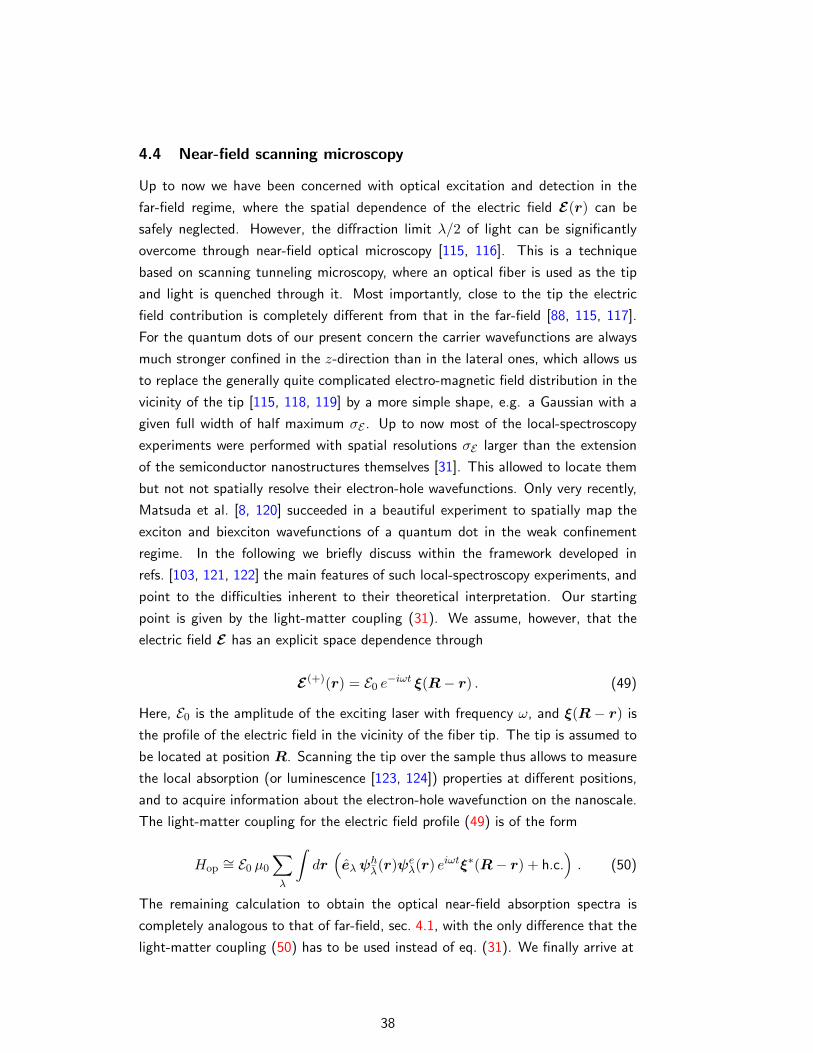
4.4 Near-field scanning microscopy

Up to now we have been concerned with optical excitation and detection in the

far-field regime, where the spatial dependence of the electric field E(r) can be

safely neglected. However, the diffraction limit λ/2 of light can be significantly

overcome through near-field optical microscopy [115, 116]. This is a technique

based on scanning tunneling microscopy, where an optical fiber is used as the tip

and light is quenched through it. Most importantly, close to the tip the electric

field contribution is completely different from that in the far-field [88, 115, 117].

For the quantum dots of our present concern the carrier wavefunctions are always

much stronger confined in the z-direction than in the lateral ones, which allows us

to replace the generally quite complicated electro-magnetic field distribution in the

vicinity of the tip [115, 118, 119] by a more simple shape, e.g. a Gaussian with a

given full width of half maximum σE . Up to now most of the local-spectroscopy

experiments were performed with spatial resolutions σE larger than the extension

of the semiconductor nanostructures themselves [31]. This allowed to locate them

but not not spatially resolve their electron-hole wavefunctions. Only very recently,

Matsuda et al. [8, 120] succeeded in a beautiful experiment to spatially map the

exciton and biexciton wavefunctions of a quantum dot in the weak confinement

regime. In the following we briefly discuss within the framework developed in

refs. [103, 121, 122] the main features of such local-spectroscopy experiments, and

point to the difficulties inherent to their theoretical interpretation. Our starting

point is given by the light-matter coupling (31). We assume, however, that the

electric field E has an explicit space dependence through

E(+)(r) = E0 e−iωt ξ(R− r) . (49)

Here, E0 is the amplitude of the exciting laser with frequency ω, and ξ(R − r) is

the profile of the electric field in the vicinity of the fiber tip. The tip is assumed to

be located at position R. Scanning the tip over the sample thus allows to measure

the local absorption (or luminescence [123, 124]) properties at different positions,

and to acquire information about the electron-hole wavefunction on the nanoscale.

The light-matter coupling for the electric field profile (49) is of the form

Hop∼= E0 µ0

∑λ

∫dr(eλψ

hλ(r)ψe

λ(r) eiωtξ∗(R− r) + h.c.). (50)

The remaining calculation to obtain the optical near-field absorption spectra is

completely analogous to that of far-field, sec. 4.1, with the only difference that the

light-matter coupling (50) has to be used instead of eq. (31). We finally arrive at

38

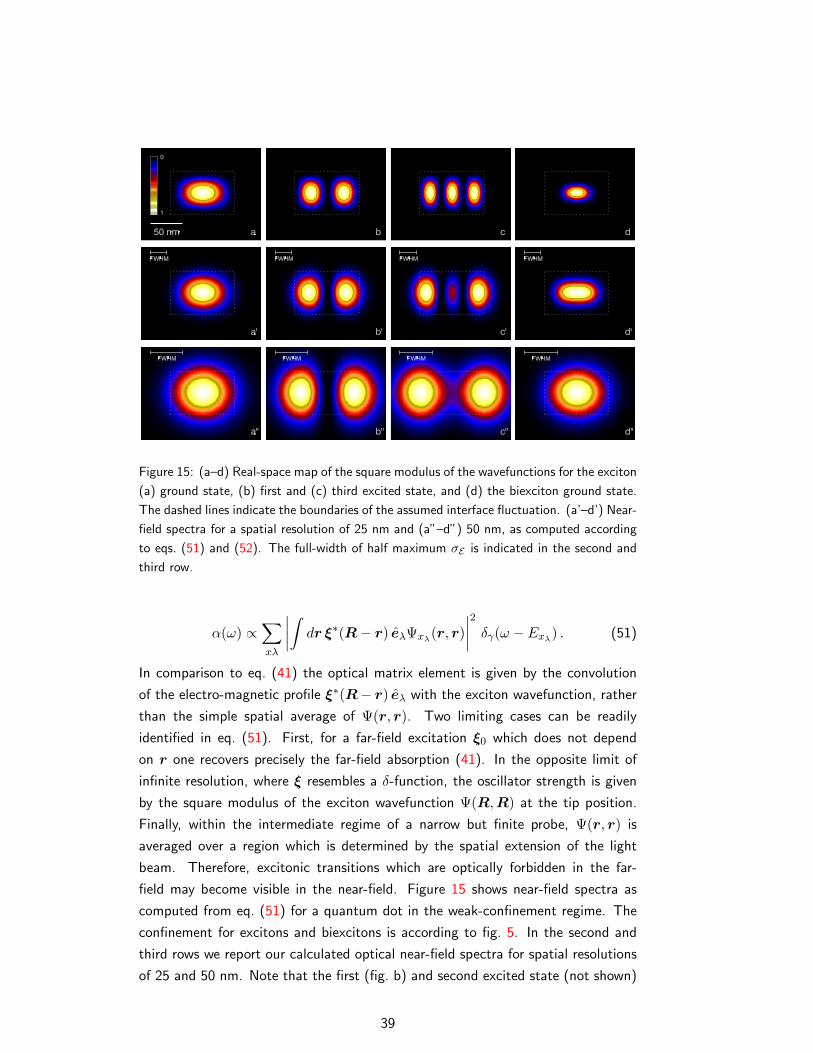
Figure 15: (a–d) Real-space map of the square modulus of the wavefunctions for the exciton

(a) ground state, (b) first and (c) third excited state, and (d) the biexciton ground state.

The dashed lines indicate the boundaries of the assumed interface fluctuation. (a’–d’) Near-

field spectra for a spatial resolution of 25 nm and (a”–d”) 50 nm, as computed according

to eqs. (51) and (52). The full-width of half maximum σE is indicated in the second and

third row.

α(ω) ∝∑xλ

∣∣∣∣∫ dr ξ∗(R− r) eλΨxλ(r, r)

∣∣∣∣2 δγ(ω − Exλ) . (51)

In comparison to eq. (41) the optical matrix element is given by the convolution

of the electro-magnetic profile ξ∗(R− r) eλ with the exciton wavefunction, rather

than the simple spatial average of Ψ(r, r). Two limiting cases can be readily

identified in eq. (51). First, for a far-field excitation ξ0 which does not depend

on r one recovers precisely the far-field absorption (41). In the opposite limit of

infinite resolution, where ξ resembles a δ-function, the oscillator strength is given

by the square modulus of the exciton wavefunction Ψ(R,R) at the tip position.

Finally, within the intermediate regime of a narrow but finite probe, Ψ(r, r) is

averaged over a region which is determined by the spatial extension of the light

beam. Therefore, excitonic transitions which are optically forbidden in the far-

field may become visible in the near-field. Figure 15 shows near-field spectra as

computed from eq. (51) for a quantum dot in the weak-confinement regime. The

confinement for excitons and biexcitons is according to fig. 5. In the second and

third rows we report our calculated optical near-field spectra for spatial resolutions

of 25 and 50 nm. Note that the first (fig. b) and second excited state (not shown)

39

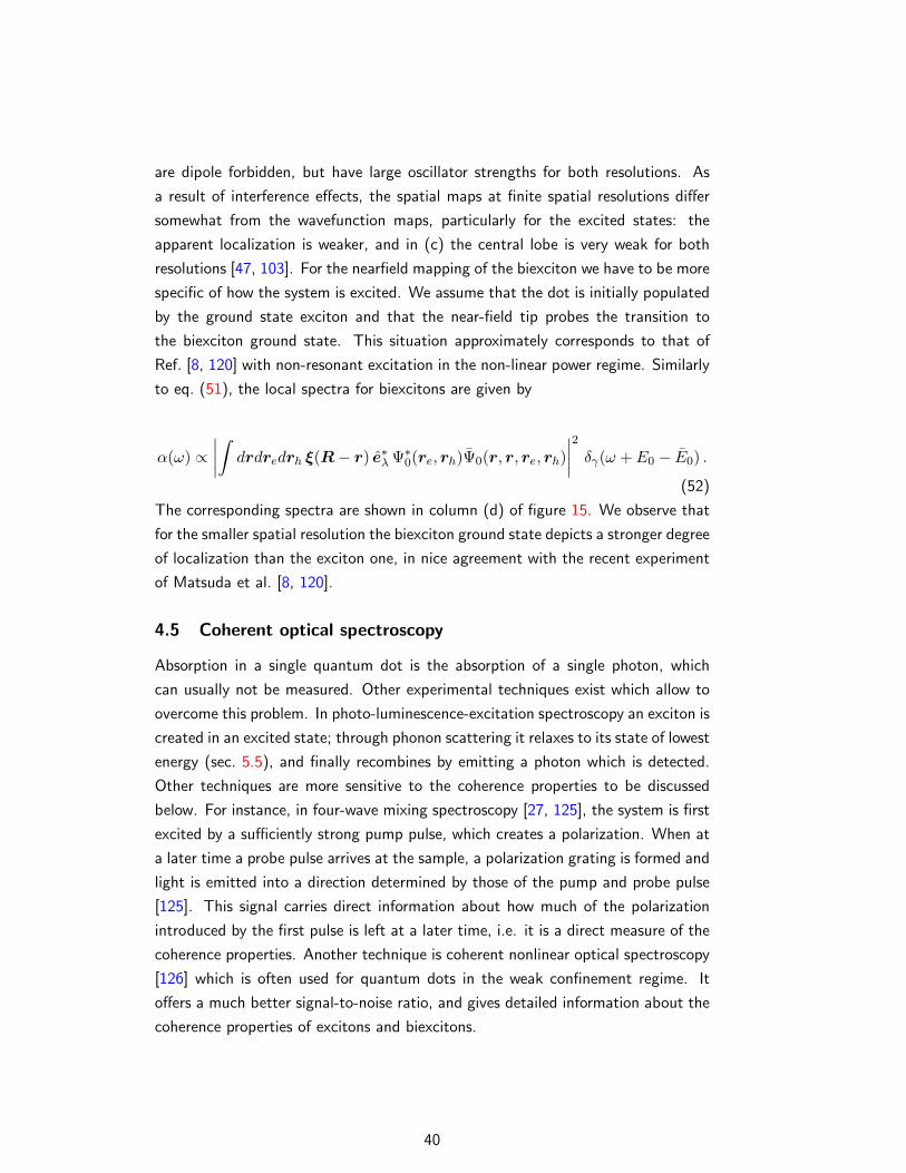
are dipole forbidden, but have large oscillator strengths for both resolutions. As

a result of interference effects, the spatial maps at finite spatial resolutions differ

somewhat from the wavefunction maps, particularly for the excited states: the

apparent localization is weaker, and in (c) the central lobe is very weak for both

resolutions [47, 103]. For the nearfield mapping of the biexciton we have to be more

specific of how the system is excited. We assume that the dot is initially populated

by the ground state exciton and that the near-field tip probes the transition to

the biexciton ground state. This situation approximately corresponds to that of

Ref. [8, 120] with non-resonant excitation in the non-linear power regime. Similarly

to eq. (51), the local spectra for biexcitons are given by

α(ω) ∝∣∣∣∣∫ drdredrh ξ(R− r) e∗λ Ψ∗

0(re, rh)Ψ0(r, r, re, rh)∣∣∣∣2 δγ(ω + E0 − E0) .

(52)

The corresponding spectra are shown in column (d) of figure 15. We observe that

for the smaller spatial resolution the biexciton ground state depicts a stronger degree

of localization than the exciton one, in nice agreement with the recent experiment

of Matsuda et al. [8, 120].

4.5 Coherent optical spectroscopy

Absorption in a single quantum dot is the absorption of a single photon, which

can usually not be measured. Other experimental techniques exist which allow to

overcome this problem. In photo-luminescence-excitation spectroscopy an exciton is

created in an excited state; through phonon scattering it relaxes to its state of lowest

energy (sec. 5.5), and finally recombines by emitting a photon which is detected.

Other techniques are more sensitive to the coherence properties to be discussed

below. For instance, in four-wave mixing spectroscopy [27, 125], the system is first

excited by a sufficiently strong pump pulse, which creates a polarization. When at

a later time a probe pulse arrives at the sample, a polarization grating is formed and

light is emitted into a direction determined by those of the pump and probe pulse

[125]. This signal carries direct information about how much of the polarization

introduced by the first pulse is left at a later time, i.e. it is a direct measure of the

coherence properties. Another technique is coherent nonlinear optical spectroscopy

[126] which is often used for quantum dots in the weak confinement regime. It

offers a much better signal-to-noise ratio, and gives detailed information about the

coherence properties of excitons and biexcitons.

40

5 Quantum coherence and decoherence

Quantum coherence and decoherence are the two key players in the fields of quan-

tum optics and semiconductor quantum optics. The light-matter coupling (32) is

mediated by the interband polarization which, in a microscopic description, cor-

responds to a coherent superposition of quantum states. For isolated systems

this provides a unique means for quantum control, where the system wavefunc-

tion can be brought to any desired state [127]. Decoherence is the process that

spoils such ideal performance. It is due to the fact that any quantum system in-

teracts with its environment, e.g. photons or phonons, and hereby acquires an

uncontrollable phase. This introduces a kind of “random noise” and diminishes the

quantum-coherence properties. While from a pure quantum-control or quantum-

computation perspective decoherence is often regarded as “the enemy” [128], from

a more physics-oriented perspective it is the grain of salt: not only it provides a

means to monitor the state of the system, but also allows for deep insights to the

detailed interplay of quantum systems with their environment. This section is de-

voted to a more careful analysis of these two key players. We first briefly review

the basic concepts of light-induced quantum coherence and its loss due to environ-

ment couplings. Based on this discussion, we then show how decoherence can be

directly monitored in optical spectroscopy and how it can be successfully exploited

for single-photon devices.

5.1 Quantum coherence

In most cases we do not have to consider the full spectrum of quantum-dot states.

For instance, if the laser frequencies are tuned to the exciton groundstate it com-

pletely suffices to know the energy of the exciton together with the optical matrix

element connecting the states. It is physical intuition together with the proper

choice of the excitation scenario which allows to reduce a complicated few-particle

problem to a relatively simple few-level scheme. This situation is quite different as

compared to the description of carrier dynamics in higher-dimensional semiconduc-

tors, where such a clear-cut separation is not possible because of the scattering-type

nature of carrier-carrier interactions [12, 27, 125]. It is, however, quite similar to

quantum optics [15, 22, 89] which relies on phenomenological level schemes, e.g. Λ-

or V-type schemes, with a few effective parameters — a highly successful approach

despite the tremendously complicated nature of atomic states. Let us denote the

generic few-level scheme with |i〉, where i labels the different states under con-

sideration. If the artificial atom would be isolated from its environment we could

describe it in terms of the wavefunction

41

|Ψ〉 =∑

i

Ci|i〉 , (53)

with Ci the coefficients subject to the normalization condition∑

i |Ci|2 = 1. Such

wavefunction description is no longer possible for a system in contact with its envi-

ronment. Because the coefficients Ci acquire random phases through environment

couplings and the system can suffer scatterings, we can only state with a certain

probability that the system is in a given state. In statistical physics this lack of

information is accounted for by the density operator [129]

ρ =∑

k

pk|Ψk〉〈Ψk| = |Ψ〉〈Ψ| , (54)

where the sum of k extends over an ensemble of systems which are with probability

pk in the state |Ψk〉. The last term on the right-hand side provides the usual short-

hand notation of this ensemble average. By construction, ρ is a hermitian operator

whose time evolution is given by the Liouville von-Neumann equation iρ = [H,ρ].This can be easily proven by differentiating eq. (54) with respect to time and using

Schrodinger’s equation for the hamiltonian H [12, 15, 129]. If we insert the few-

level wavefunctions (53) into (54) we obtain

ρ =∑ij

CiC∗j |i〉〈j| =

∑ij

ρij |i〉〈j| . (55)

Here, ρij = CiC∗j is the density matrix of the few-level system which contains the

maximum information we possess about the system. The diagonal elements ρii

account for the probability of finding the system in state i, and the off-diagonal

elements ρij for the quantum coherence between states i and j. As consequence

ρ fulfills the trace relation trρ =∑

i ρii = 1 which states that the system has to

be in one of its states.

5.1.1 Two-level system

A particularly simple and illustrative example is given by a generic two-level system.

This may correspond to an artificial atom that is either in its groundstate 0 or in

the single-exciton state 1. In optical experiments the population of excited exciton

states can be strongly suppressed through appropriate frequency filtering (recall

that the principal level splittings are of the order of several tens of meV), and that

of biexcitons through appropriate light polarization. Thus, systems with dominant

two-level character can indeed be identified in artificial atoms. The density matrix

is of dimension two. It has four complex matrix elements corresponding to eight

real numbers. Because ρ is a hermitian matrix only four of them are independent,

42

which additionally have to fulfill the normalization condition trρ = 1. A convenient

representation of ρ is through the Pauli matrices

σ1 = |1〉〈0|+ |0〉〈1|, σ2 = −i (|1〉〈0| − |0〉〈1|) , σ3 = |1〉〈1| − |0〉〈0| , (56)

which together with the unit matrix 11 = |1〉〈1| + |0〉〈0| provide a complete basis

within the two-level subspace. The Pauli matrices are hermitian and have trace

zero (appendix C). Thus, the density matrix can be expressed as

ρ =12

(11 +

∑i

ui σi

)=

12

(11 + uσ) , (57)

with σ = (σ1, σ2, σ3) and the first term guarantees the trace relation trρ = 1.

The system is thus fully characterized by the three-dimensional Bloch vector u =(u1, u2, u3) which was already introduced in sec. 2.3: its x- and y-components

u1 and u2 account for the real and imaginary part of the quantum coherence —or

interband polarization—, respectively, and the z-component u3 gives the population

inversion between the excited and ground state. Equation (57) demonstrates that

the Bloch-vector picture advocated in sec. 2 prevails for density matrices. What

happens when the system is excited by an external laser? As discussed in appendix

C, within a rotating frame the system subject to an exciting laser can be described

by the hamiltonian [22]

H =12

(∆σ3 − Ω∗ |0〉〈1| − Ω |1〉〈0|

), (58)

where ∆ is the detuning between the laser and the two-level transition, and Ω is

the Rabi frequency which determines the strength of the light-matter coupling.

Note that Ω describes the envelope part of the laser pulse which is constant for

a constant laser and has an only small time dependence for typical pulses. From

the Liouville von-Neumann equation ρ = −i[H,ρ] we then obtain the equation of

motion for the Bloch vector

u = Ω× u, Ω = (−<e(Ω),=m(Ω),∆) . (59)

We are now in the position to quantitatively describe the buildup of quantum

coherence. Suppose that the system is initially in its groundstate 0 where the

Bloch vector points into the negative z-direction. When the laser is turned on, the

Bloch vector is rotated perpendicularly to Ω. Upon expansion of the solutions of

the Bloch equations (59) in powers of the driving field Ω, we observe that to the

lowest order the population, i.e. the z-component of the Bloch vector, remains

unchanged and only a quantum coherence —described by u1 and u2— is created.

43

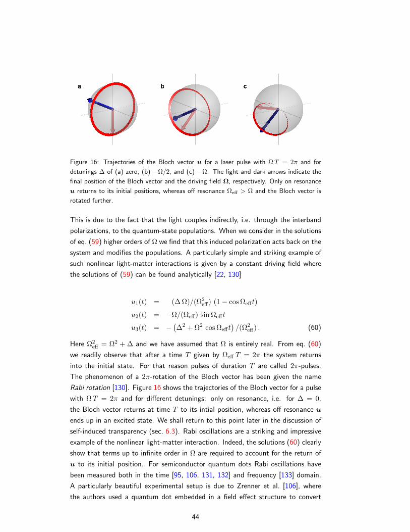
Figure 16: Trajectories of the Bloch vector u for a laser pulse with ΩT = 2π and for

detunings ∆ of (a) zero, (b) −Ω/2, and (c) −Ω. The light and dark arrows indicate the

final position of the Bloch vector and the driving field Ω, respectively. Only on resonance

u returns to its initial positions, whereas off resonance Ωeff > Ω and the Bloch vector is

rotated further.

This is due to the fact that the light couples indirectly, i.e. through the interband

polarizations, to the quantum-state populations. When we consider in the solutions

of eq. (59) higher orders of Ω we find that this induced polarization acts back on the

system and modifies the populations. A particularly simple and striking example of

such nonlinear light-matter interactions is given by a constant driving field where

the solutions of (59) can be found analytically [22, 130]

u1(t) = (∆ Ω)/(Ω2eff) (1− cos Ωefft)

u2(t) = −Ω/(Ωeff) sin Ωefft

u3(t) = −(∆2 + Ω2 cos Ωefft

)/(Ω2

eff) . (60)

Here Ω2eff = Ω2 + ∆ and we have assumed that Ω is entirely real. From eq. (60)

we readily observe that after a time T given by Ωeff T = 2π the system returns

into the initial state. For that reason pulses of duration T are called 2π-pulses.

The phenomenon of a 2π-rotation of the Bloch vector has been given the name

Rabi rotation [130]. Figure 16 shows the trajectories of the Bloch vector for a pulse

with ΩT = 2π and for different detunings: only on resonance, i.e. for ∆ = 0,

the Bloch vector returns at time T to its intial position, whereas off resonance u

ends up in an excited state. We shall return to this point later in the discussion of

self-induced transparency (sec. 6.3). Rabi oscillations are a striking and impressive

example of the nonlinear light-matter interaction. Indeed, the solutions (60) clearly

show that terms up to infinite order in Ω are required to account for the return of

u to its initial position. For semiconductor quantum dots Rabi oscillations have

been measured both in the time [95, 106, 131, 132] and frequency [133] domain.

A particularly beautiful experimental setup is due to Zrenner et al. [106], where

the authors used a quantum dot embedded in a field effect structure to convert

44

the final exciton population to a photocurrent which could be directly measured.

A somewhat different approach was pursued by Kamada et al. [133] where the

appearance of additional peaks in the resonance-luminescence spectra at frequencies

ω0±Ωeff centered around the laser frequency ω0 were observed — a clear signature

of Rabi-type oscillations [15, 22]. We conclude this section with a short comment

on the coherence properties of the Bloch-vector propagation. In fact, the time

evolution (60) of the isolated quantum system can be described in terms of the

projector ρ = |Ψ〉〈Ψ|, where |Ψ〉 is the system wavefunction. Such projector-like

density operators have the unique property ρ2 = ρ. For the two-level system under

consideration this has the consequence that the length of the Bloch vector remains

one throughout. In other words, the trajectory of u is located on the surface of the

Bloch sphere (figs. 3 and 16), i.e. the unit sphere in the Bloch space.

5.2 Decoherence

Decoherence describes the process where a quantum system in contact with its

environment loses its quantum-coherence properties. We shall assume that the

environment —sometimes referred to as a reservoir— has an infinite number of

degrees of freedom, and we are not able to precisely specify the corresponding

statevector. To account for this lack of information, in the following we adopt the

framework of statistical physics. Suppose that the problem under consideration

is described by the hamiltonian HS + HR + V , where HS and HR account for

the system and reservoir, respectively, and V for their coupling. Let w(t) be the

density operator of the total system in the interaction representation according to

HS +HR. The quantity of interest is the reduced density operator ρ of the system

alone. It is obtained from the total density operator by tracing over the reservoir

degrees of freedom through ρ = trRw. We shall now derive the equation of motion

for ρ when it is in contact with the environment. As a starting point we trace in

the Lioville von-Neumann equation for w over the reservoir degrees of freedom and

obtain

ρ(t) = trR w(t) = −i trR [V (t),w(t)] . (61)

The important feature of this equation is that we are only able to trace out the

reservoir on the left-hand side but not on the right-hand side which still depends

on the full density operator w. The simple and physical deep reason for this is that

through V the system and environment become entangled and can no longer be

described independently. Suppose that at an early time t0 system and reservoir were

uncorrelated such that w(t0) = ρ(t0)⊗ ρR, with ρR is the density operator of the

reservoir. We can then use the usual time evolution operator U(t, t0) to establish

45

a relation between w(t) and w(t0). To the lowest order in the system-environment

coupling V we find [89]

w(t) = w(t0)−∫ t

t0

dt′[V (t′),ρ(t0)⊗ ρR

]+O(V 2) . (62)

This expression no longer depends on the density operator w(t) of the interacting

system and environment. We can thus insert eq. (62) into (61) to obtain an equa-

tion of motion for ρ which depends on the system degrees of freedom only. One

additional approximation proves to be useful. To the same order in the system-

environment interaction V one can replace ρ(t0) by ρ(t) [89] — a well-defined

procedure which can be justified for any given order of V [134, 135]. This replace-

ment is known as the Markov approximation and has the advantage that the time

evolution of the density operator ρ(t) only depends on its value at the same instant

of time. Then,

ρ(t) ∼= −∫ t

t0

dt′ trR[V (t),

[V (t′),ρR ⊗ ρ(t)

]], (63)

and we have made the assumption trR [V,ρ(t0) ⊗ ρR] = 0 which holds true in

most cases of interest [15, 89]. Equation (63) is our final result. It has the evident

structure that at time t′ the system becomes entangled with the environment, the

entangled system and reservoir propagate for a while —note that V is given in the

interaction representation according to HS +HR—, and finally a back-action on the

system occurs at time t. Because of the finite interaction time, within the processes

of decoherence and relaxation the system can acquire an uncontrollable phase or can

exchange energy with the environment. The general structure of eq. (63) prevails

if higher orders of the interaction V are considered [136, 137, 138, 139], as will be

also discussed at the example of phonon-assisted dephasing in sec. 5.5.

5.2.1 Caldeira-Leggett-type model

To be more specific, in the following we consider the important case where a generic

two-level system is coupled linearly to a bath of harmonic oscillators [140, 141, 142]

H =E0

2σ3 +

∑i

ωi a†iai + i

∑i

gi

(a†i σ− − ai σ+

). (64)

Here, E0 is the energy splitting between ground and excited state, ωi the energies

of the harmonic oscillators which are described by the bosonic field operator ai, and

gi the system-oscillator coupling constant which is assumed to be real. The last

term on the right-hand side defines the system-environment interaction V where

we have introduced the lowering and raising operators σ− = |0〉〈1| and σ+ = |1〉〈0|

46

for the two-level system. If we insert V in the interaction representation according

to HS +HR into eq. (63) we obtain

ρ(t) ∼= −∫ t

t0

dt′∑ij

gigj

(⟨ai(t)a

†j(t

′)⟩σ+(t)σ−(t′)ρ(t) +

⟨aj(t′)a

†i (t)⟩ρ(t)σ+(t′)σ−(t)

−⟨ai(t)a

†j(t

′)⟩σ−(t′)ρ(t)σ+(t)−

⟨aj(t′)a

†i (t)⟩σ−(t)ρ(t)σ+(t′)

+⟨a†i (t)aj(t′)

⟩σ−(t)σ+(t′)ρ(t) +

⟨a†j(t

′)ai(t)⟩ρ(t)σ−(t′)σ+(t)

−⟨a†i (t)aj(t′)

⟩σ+(t′)ρ(t)σ−(t)−

⟨a†j(t

′)ai(t)⟩σ+(t)ρ(t)σ−(t′)

).

(65)

Here, the terms in brackets have been derived by use of cyclic permutation under the

trace and describe the propagation of excitations in the environment. The remaining

terms with ρ and σ account for the effects of environment coupling on the system.

The expression in the second and third line describe emission processes where an

environment excitation is created prior to its destruction, and those in the fourth

and fifth line absorption processes where the destruction is prior to the creation.

The latter processes usually only occur at finite temperatures. In the following we

suppose that ρR describes the reservoir in thermal equilibrium such that 〈a†iaj〉 ∼=δij n(ωi), with n(ω) the usual Bose-Einstein distribution function. Within this spirit

we have also neglected in eq. (65) terms with 〈aa〉 and 〈a†a†〉 which would only

play a role in specially prepared environments such as squeezed reservoirs [89]. Let

us next consider one specific term in (65), which can be simplified according to

∫ t−t0

0dτ∑ij

gigj

⟨ai(τ)a

†j(0)

⟩eiE0τ ∼=

∑i

g2i (1 + n(ωi)) γ(E0 − ω, t− t0) ,

(66)

with γ(Ω, t) = sinΩt/Ω (and we have neglected terms which only contribute

to energy renormalizations but not to decoherence and relaxation [89]). γ(Ω, t)has the important feature that in the adiabatic limit limt→∞ γ(Ω, t) = πδ(Ω) it

gives Dirac’s delta function. Thus, for sufficiently long times the various terms

in eq. (65) account for energy-conserving scattering processes (as discussed be-

low the strict adiabatic t → ∞ limit is usually not needed and it suffices to

assume that the reservoir memory is sufficiently short-lived). Within the adia-

batic limit the environment couplings can then be described by the scattering rates

Γ1 = 2π∑

i g2i (1 + n(ωi)) δ(ωi − E0) and Γ2 = 2π

∑i g

2i n(ωi) δ(ωi − E0) for

emission and absorption, respectively, and the Lindblad operators L1 =√

Γ1 σ−

47

and L2 =√

Γ2 σ+ associated to emission and absorption. We can bring eq. (65)

to the compact form

ρ = −i(Heffρ− ρH†eff) +

∑i

LiρL†i , (67)

where Heff = HS−(i/2)∑

i L†iLi is an effective, non-hermitian hamiltonian. Equa-

tion (67) is known as a master equation of Lindblad form [89, 143]. It has the

intriguing feature that it is guaranteed that during the time evolution the trace

over ρ remains one throughout.

5.2.2 Unraveling of the master equation

In many cases of interest the master equation (67) of Lindblad form can be solved

by a simple and particularly transparent scheme. It is known as the unraveling of

the master equation [144, 145, 146]. Recall that the density operator is a statistical

mixture of state vectors, ρ =∑

k pk |Ψk〉〈Ψk|, where the summation over k results

from the statistical average of the various pure states |Ψk〉. For simplicity we

restrict ourselves to a single state vector |Ψ〉. The general case (54) then follows

from a straightforward generalization. On insertion of the projector |Ψ〉〈Ψ| into the

master equation (67) we obtain

d

dt|Ψ〉〈Ψ| = −i

(Heff |Ψ〉〈Ψ| − |Ψ〉〈Ψ|H†

eff

)+∑

i

Li |Ψ〉〈Ψ|L†i . (68)

The first term on the right-hand side can be interpreted as a non-hermitian,

Schrodinger-like evolution i|Ψ〉 = Heff |Ψ〉 under the influence of Heff . In contrast,

the second term describes a time evolution where |Ψ〉 is projected —or jumps— to

one of the possible states Li|Ψ〉. For sufficiently small time intervals δt the time

evolution according to Heff is given by |Ψ(t + δt)〉 = (1 − iHeff δt)|Ψ(t)〉. Note

that Heff is non-hermitian and consequently the wavefunction at later time is not

normalized. To the lowest order in δt the decrease of norm δp is given by

δp = iδt⟨Ψ(t)

∣∣∣Heff −H†eff

∣∣∣Ψ(t)⟩

= δt∑

i

⟨Ψ(t)

∣∣∣L†iLi

∣∣∣Ψ(t)⟩

=∑

i

δpi . (69)

The full master equation evolution has to preserve the norm. This missing norm δp

is brought in by the states Li|Ψ(t)〉 to which the system is scattered with probability

δpi. The time evolution of the density operator can thus be decomposed into

ρ(t+ δt) ∼= (1− δp)ρ0(t+ δt) + δpρ1(t+ δt) , (70)

48

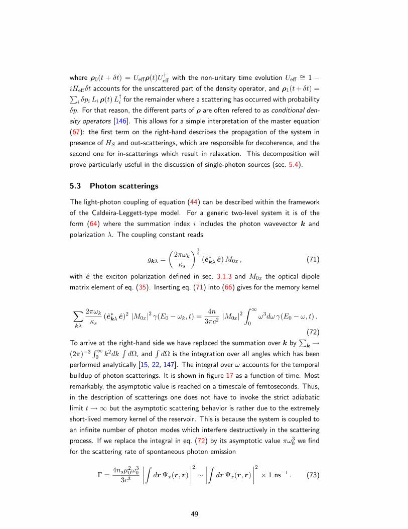
where ρ0(t + δt) = Ueffρ(t)U †eff with the non-unitary time evolution Ueff

∼= 1 −iHeffδt accounts for the unscattered part of the density operator, and ρ1(t+ δt) =∑

i δpi Li ρ(t)L†i for the remainder where a scattering has occurred with probability

δp. For that reason, the different parts of ρ are often refered to as conditional den-

sity operators [146]. This allows for a simple interpretation of the master equation

(67): the first term on the right-hand describes the propagation of the system in

presence of HS and out-scatterings, which are responsible for decoherence, and the

second one for in-scatterings which result in relaxation. This decomposition will

prove particularly useful in the discussion of single-photon sources (sec. 5.4).

5.3 Photon scatterings

The light-photon coupling of equation (44) can be described within the framework

of the Caldeira-Leggett-type model. For a generic two-level system it is of the

form (64) where the summation index i includes the photon wavevector k and

polarization λ. The coupling constant reads

gkλ =(

2πωk

κs

) 12

(e∗kλ e)M0x , (71)

with e the exciton polarization defined in sec. 3.1.3 and M0x the optical dipole

matrix element of eq. (35). Inserting eq. (71) into (66) gives for the memory kernel

∑kλ

2πωk

κs(e∗kλ e)

2 |M0x|2 γ(E0 − ωk, t) =4n

3πc2|M0x|2

∫ ∞

0ω3dω γ(E0 − ω, t) .

(72)

To arrive at the right-hand side we have replaced the summation over k by∑

k →(2π)−3

∫∞0 k2dk

∫dΩ, and

∫dΩ is the integration over all angles which has been

performed analytically [15, 22, 147]. The integral over ω accounts for the temporal

buildup of photon scatterings. It is shown in figure 17 as a function of time. Most

remarkably, the asymptotic value is reached on a timescale of femtoseconds. Thus,

in the description of scatterings one does not have to invoke the strict adiabatic

limit t→∞ but the asymptotic scattering behavior is rather due to the extremely

short-lived memory kernel of the reservoir. This is because the system is coupled to

an infinite number of photon modes which interfere destructively in the scattering

process. If we replace the integral in eq. (72) by its asymptotic value πω30 we find

for the scattering rate of spontaneous photon emission

Γ =4nsµ

20ω

30

3c3

∣∣∣∣∫ drΨx(r, r)∣∣∣∣2 ∼ ∣∣∣∣∫ drΨx(r, r)

∣∣∣∣2 × 1 ns−1 . (73)

49

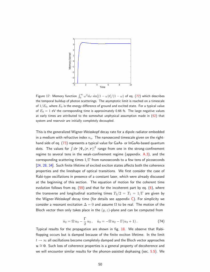
0 2 4 6 8 10−4

−3

−2

−1

0

1

2

3

4

Time

Mem

ory

kern

el

Figure 17: Memory function∫∞0ω3dω sin[(1 − ω)t]/(1 − ω) of eq. (72) which describes

the temporal buildup of photon scatterings. The asymptotic limit is reached on a timescale

of 1/E0, where E0 is the energy difference of ground and excited state. For a typical value

of E0 = 1 eV the corresponding time is approximately 0.66 fs. The large negative values

at early times are attributed to the somewhat unphysical assumption made in (62) that

system and reservoir are initially completely decoupled.

This is the generalized Wigner-Weisskopf decay rate for a dipole radiator embedded

in a medium with refractive index ns. The nanosecond timescale given on the right-

hand side of eq. (73) represents a typical value for GaAs- or InGaAs-based quantum

dots. The values for∫dr |Ψx(r, r)|2 range from one in the strong-confinement

regime to several tens in the weak-confinement regime (appendix. A.3), and the

corresponding scattering times 1/Γ from nanoseconds to a few tens of picoseconds

[24, 28, 34]. Such finite lifetime of excited exciton states affects both the coherence

properties and the lineshape of optical transitions. We first consider the case of

Rabi-type oscillations in presence of a constant laser, which were already discussed

at the beginning of this section. The equation of motion for the coherent time

evolution follows from eq. (59) and that for the incoherent part by eq. (6), where

the transverse and longitudinal scattering times T2/2 = T1 = 1/Γ are given by

the Wigner-Weisskopf decay time (for details see appendix C). For simplicity we

consider a resonant excitation ∆ = 0 and assume Ω to be real. The motion of the

Bloch vector then only takes place in the (y, z)-plane and can be computed from

u2 = Ωu3 −Γ2u2 , u3 = −Ωu2 − Γ(u3 + 1) . (74)

Typical results for the propagation are shown in fig. 18. We observe that Rabi-

flopping occurs but is damped because of the finite exciton lifetime. In the limit

t→∞ all oscillations become completely damped and the Bloch vector approaches

u ∼= 0. Such loss of coherence properties is a general property of decoherence and

we will encounter similar results for the phonon-assisted dephasing (sec. 5.5). We

50

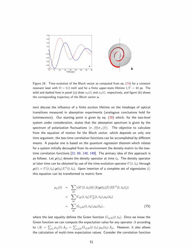
0 5 10 15 20 25 30 35 40−1

−0.8

−0.6

−0.4

−0.2

0

0.2

0.4

0.6

0.8

Time (ps)

a

Figure 18: Time evolution of the Bloch vector as computed from eq. (74) for a constant

resonant laser with Ω = 0.2 meV and for a finite upper-state lifetime 1/Γ = 40 ps. The

solid and dashed lines in panel (a) show u2(t) and u3(t), respectively, and figure (b) shows

the corresponding trajectory of the Bloch vector u.

next discuss the influence of a finite exciton lifetime on the lineshape of optical

transitions measured in absorption experiments (analogous conclusions hold for

luminescence). Our starting point is given by eq. (39) which, for the two-level

system under consideration, states that the absorption spectrum is given by the

spectrum of polarization fluctuations 〈σ−(0)σ+(t)〉. The objective to calculate

from the equation of motion for the Bloch vector, which depends on only one

time argument, the two-time correlation functions can be accomplished by different

means. A popular one is based on the quantum regression theorem which relates

for a system initially decoupled from its environment the density-matrix to the two-

time correlation functions [22, 89, 148, 149]. The primary idea of this approach is

as follows. Let ρ(t0) denote the density operator at time t0. The density operator

at later time can be obtained by use of the time evolution operator U(t, t0) through

ρ(t) = U(t, t0)ρ(t0)U †(t, t0). Upon insertion of a complete set of eigenstates |i〉this equation can be transformed to matrix form

ρij(t) =∑kl

〈i|U(t, t0)|k〉〈k|ρ(t0)|l〉〈l|U †(t, t0)|j〉

=∑kl

Uik(t, t0)U∗jl(t, t0) ρkl(t0)

=∑kl

Gij,kl(t, t0) ρkl(t0) , (75)

where the last equality defines the Green function Gij,kl(t, t0). Once we know the

Green function we can compute the expectation value for any operator A according

to 〈A〉 =∑

ij ρij(t)Aji =∑

ij,klGij,kl(t, t0) ρkl(t0)Aji. However, it also allows

the calculation of multi-time expectation values. Consider the correlation function

51

for two operators A and B in the Heisenberg picture

〈A(t)B(t0)〉 = trρ (t0)U †(t, t0)AU(t, t0)B

= 〈i|ρ(t0)|j〉〈j|U †(t, t0)|l〉〈l|A|m〉〈m|U(t, t0)|n〉〈n|B|i〉

= Umn(t, t0)U∗lj(t, t0)Bni ρij(t0)Alm

= Gml,nj(t, t0)Bni ρij(t0)Alm , (76)

where we have made use of the usual Einstein summation convention. Importantly,

eq. (76) shows that the two-time correlation function can be computed by replacing

the density-matrix ρij(t0) at time t0 by the modified expression∑

k Bik ρkj(t0).The result, which is know as the quantum regression theorem, implies that the

fluctuations regress in time like the macroscopic averages. Equation (76) holds

exactly but the factorization of the density operator at time t0 plays an essential

role in the derivation [22]. We shall now show how this result can be used to

compute the polarization fluctuations 〈σ−(t)σ+(t0)〉. According to the regression

theorem we have to use instead of the initial density operator ρ(t0) = |0〉〈0| the

modified σ+ ρ(t0) = |1〉〈0| = σ+ one. Inserting σ+ into the Lindblad equation

(67) gives

σ+ = −i(E0 − i

Γ2

)σ+ , (77)

which shows that the excitation σ+ propagates with the transition energy E0 but

is damped because of spontaneous photon emissions. For the correlation function

we obtain 〈σ−(t)σ+(t0)〉 = exp−i[E0− i(Γ/2)](t− t0) which, upon insertion into

eq. (39), gives the final result

α(ω) ∝ Γ/2(ω − E0)2 + (Γ/2)2

. (78)

The lineshape for optical transitions of a two-level system subject to spontaneous

photon emissions is a Lorentzian centered at E0 and with a full-width of half

maximum of Γ/2. In a nonlinear coherent-spectroscopy experiment Bonadeo et al.

[26] made the important observation that for excitons in the weak-confinement

regime energy relaxation and dephasing rates are comparable and predominantly

due to photon emissions, thus reflecting the absence of significant pure dephasing.

Such behavior is quite surprising for the solid state since all interaction mechanisms

can contribute to T2 but only a few to T1. Similar results were also found in the

strong confinement regime where, however, things turn out to be more complicated

(sec. 5.5) [24, 34, 83, 150, 151].

52

5.4 Single-photon sources

Single-photon sources are one of the most promising quantum-dot based quantum

devices. The creation of a single photon on demand —first a trigger is pushed and

one single photon is emitted after a given time interval— plays an important role in

quantum cryptography, e.g. for secure key distributions [19, 21]. Gerard and Gayral

[152] were the first to propose a turnstile single-photon source based on artificial

atoms. Their proposal exploits two peculiarities of artificial atoms: first, because of

Coulomb renormalizations of the few-particle states in the decay of a multi-exciton

state each photon is emitted at a different frequency (see fig. 14); second, because

of environment couplings —for details see below— photons are always emitted

from the few-particle state of lowest energy. Thus, in the cascade decay of a multi-

exciton complex the last photon will always be that of the single-exciton decay, and

this photon can be distinguished from the others through spectral filtering. This

is how the quantum-dot based single-photon source works: a short pump laser ex-

cites electron-hole pairs in the continuum states in the vicinity of the quantum dot,

where some become captured in the dot; the resulting multi-exciton complex decays

by emitting photons — because of Coulomb renormalizations each photon has a

different frequency and because of environment couplings emission only takes place

from the respective few-particle states of lowest energy; finally, the “single photon

on demand” comes from the last single-exciton decay. Spectral filtering of the last

photon is usually accomplished by placing the quantum dot in an optical resonator

such as a microcavity [153, 154]. The theoretical description of single scatterings is

a quite non-trivial task. The framework of environment couplings developed in this

section is based on statistical physics and thus applies to ensembles of (identical)

systems only. How do things have to be modified for the description of a single

system? Surprisingly enough not too much. The question of how to theoretically

describe such problems first arose almost two decades ago when it became possible

to store single ions in a Paul trap and to continuously monitor their resonance flu-

orescence, and led to the development of the celebrated quantum-jump approach

[144, 145, 146]. This approach combines the usual master-equation approach with

the rules of demolition quantum measurements [146, 155] and provides a flexible

tool for the description of single-system dynamics subject to continuous monitor-

ing. Suppose that the artificial atom and the photon environment at time t0 are

described by the density operator w(t0) = ρ(t0)⊗ρR. We shall now let the system

evolve for a short time δt in presence of the light-matter coupling. This time δt is

supposed to be long enough to allow the photon to become separated from the dot

—see fig. 17 for the buildup time of scatterings—, and short enough that only a

single photon is emitted. What is the probability that a photon is detected within

53

δt? Let P0 = |0R〉〈0R| denote the projector on the photon vacuum 0R. Then

P0 = tr P0 U(t0 + δt, t0)w(t0)U †(t0, t0 + δt) P0 (79)

gives the probability that within δt no photon is emitted. The term UwU † de-

scribes the propagation of the quantum dot coupled to photons, and the projection

operators P0 the photon detection. With probability P0 no photon is detected. If

we correspondingly project in eq. (79) on the single-photon subspace P1 we get

the probability P1 that one photon is detected within δt. Obviously P0 + P1 = 1must be fulfilled. There is one important conclusion to be drawn from eq. (79).

If we compute according to eq. (63) the time evolution of the density operator to

the lowest order in V , but replace the trace over the reservoir by the projection

operators P0 and P1 —which are associated to the outcome of the measurement—

we encounter expressions which are completely similar to those of the emission

processes in the second and third line of eq. (65). However, the terms in the

second line only show up for projection on P0 and those in the third line only for

projection on P1. This dependence can be understood as follows. In the quantum-

mechanical time evolution (63) of the master equation the density operator splits

up into two terms associated to the situations where a photon is emitted or not.

Through the measurement —described by the projection operators P0 and P1—

we acquire additional information whether a photon has been emitted or not, and

we corrispondingly have to modify the density operator. A particularly transparent

description scheme for this propagation subject to quantum measurements is given

by the master equation (67) of Lindblad form and its unraveling (70) [146, 155]. In

the time evolution of ρ(t) we assume that after each time interval δt a gedanken

measurement is performed [146, 155], where either no photon or a single photon

is detected. These two situations correspond to the two terms of eq. (70) with

probabilities P0 = 1 − δp and P1 = δp. The decomposition of the time evolution

of the density operator into no-scattering and scattering contributions provides an

elegant means to calculate probabilities for finite time intervals [t0, t]. Let us intro-

duce the conditional density operator ρ0, associated to no-photon detection, whose

time evolution is given by

ρ0 = −i(Heff ρ0 − ρ0H

†eff

), (80)

subject to the initial condition ρ0(t0) = ρ(t0). Because Heff is a non-hermitian

operator, the trace P0(t) = trρ0(t) decreases and gives the probability that the

system has not emitted a photon within [t0, t]. The probability that a photon is

emitted at t is given by −δt P0(t). Once a photon has been detected, we acquire

additional information about the system, and accordingly have to change its density

54

operator. This is the point where the second term of the unraveled master equation

(70) comes into play. For the photon emission described by the Lindblad operator

Li (i may correspond to the photon polarization),

ρ(t+ δt) −→Liρ0(t)L

†i

tr[Liρ0(t)L†i ]

(81)

gives the density operator right after the scattering (the denominator guarantees

that the density operator after the scattering fulfills the trace relation). Table 4 lists

some of the basic quantities of this scheme which is known as the quantum-jump

approach [146]. Let us consider as a first example the situation where a quantum

dot is initially in the single-exciton state. With the Lindblad operator L =√

Γσ−associated to photon emission, we obtain for the effective hamiltonian Heff =−i(Γ/2)|1〉〈1|. Thus the decay of P0(t) = exp−Γt is mono-exponentially and the

probability to detect a photon at time t is given by −δt P0(t) = δtΓ exp−Γt.

Photon antibunching. We next consider the situation where a single quantum

dot is driven by a constant laser with Rabi frequency Ω, and the resonance lu-

minescence —sometime refered to as resonance fluorescence— is measured. The

quantity we are interested in is the probability that once a photon has been de-

tected at time zero the next photon is detected at time t. It is similar to the

two-photon correlation function g(2)(t) [15, 22, 146], with the only difference that

we ask for the next instead of any subsequent photon. With the framework of

the quantum-jump approach we are in the position to readily compute things.

This is how it goes. Suppose that the system is initially in state |0〉. The ef-

fective hamiltonian in presence of the driving laser and of photon emissions is

Heff = (1/2)[∆σ3 −Ωσ1 − iΓ(11 + σ3)/2], with ∆ the detuning between the laser

and the two-level transition which we assume to be zero. As shown in appendix C,

the probability P0(t) for no-photon emission can then be computed analytically

P0(t) = e− sinh θ Ωeff t(1 + sinh θ sinΩefft

), (82)

where Ω2eff = Ω2 − (Γ/2)2 for Ω > Γ/2 and we have defined the angle θ through

tanh θ = (Γ/2Ω). Equation (82) gives the probability that a system —which is

initially in its groundstate and is subject to a constant laser field— has emitted

no photon within [0, t]. Small angles θ refer to the case that photon scatterings

occur seldomly on the time scale of 1/Ω, and large angles to the case where photon

emissions and Rabi flopping take place on the same time scale. Figure 19a shows

P0(t) as computed from eq. (82) for different values of θ. We observe that in

all cases P0(t) decays exponentially —the decay constant is given by sinh θΩeff—

and is modulated by the Rabi-type oscillations of sinΩefft. The latter oscillations

55

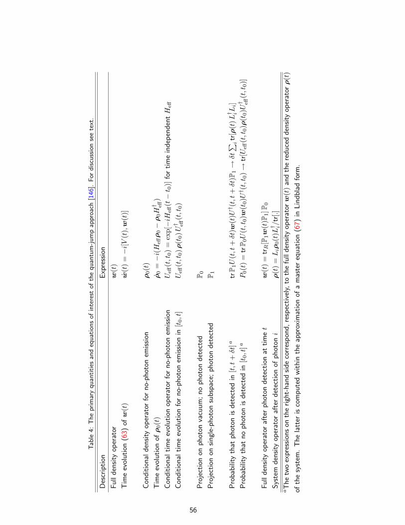
Tab

le4:

The

prim

ary

quan

tities

and

equat

ions

ofin

tere

stof

the

quan

tum

-jum

pap

proa

ch[1

46].

For

discu

ssio

nse

ete

xt.

Des

crip

tion

Exp

ress

ion

Full

den

sity

oper

ator

w(t

)T

ime

evol

ution

(63)

ofw

(t)

w(t

)=−i[V

(t),w

(t)]

Con

ditio

nal

den

sity

oper

ator

for

no-

phot

onem

ission

ρ0(t

)T

ime

evol

ution

ofρ

0(t

)ρ

0=−i(H

effρ

0−ρ

0H† eff

)Con

ditio

nal

tim

eev

olution

oper

ator

for

no-

phot

onem

ission

Ueff

(t,t

0)

=ex

p[−iH

eff(t−t 0

)]fo

rtim

ein

dep

enden

tH

eff

Con

ditio

nal

tim

eev

olution

for

no-

phot

onem

ission

in[t

0,t

]U

eff(t,t

0)ρ

(t0)U

† eff(t,t

0)

Pro

ject

ion

onphot

onva

cuum

;no

phot

ondet

ecte

dP 0

Pro

ject

ion

onsingl

e-phot

onsu

bsp

ace;

phot

ondet

ecte

dP 1

Pro

bab

ility

that

phot

onis

det

ecte

din

[t,t

+δt

]atr

P 1U

(t,t

+δt

)w(t

)U† (t,t+δt

)P1→δt∑ i

tr[ρ

(t)L

† iL

i]Pro

bab

ility

that

no

phot

onis

det

ecte

din

[t0,t

]aP

0(t

)=

trP 0U

(t,t

0)w

(t0)U

† (t,t 0

)→

tr[U

eff(t,t

0)ρ

(t0)U

† eff(t,t

0)]

Full

den

sity

oper

ator

afte

rphot

ondet

ection

attim

et

w(t

)=

trR[P

1w

(t)P

1]P

0

Sys

tem

den

sity

oper

ator

afte

rdet

ection

ofphot

oni

ρ(t

)=L

iρ0(t

)L† i/tr

[.]aT

he

two

expr

ession

son

the

righ

t-han

dside

corr

espon

d,re

spec

tive

ly,to

the

full

den

sity

oper

atorw

(t)

and

the

reduce

dden

sity

oper

atorρ(t

)of

the

syst

em.

The

latt

eris

com

pute

dw

ithin

the

appr

oxim

atio

nof

am

aste

req

uat

ion

(67)

inLin

dbla

dfo

rm.

56

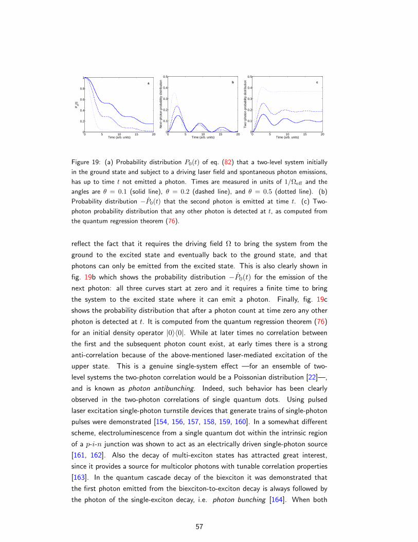
0 5 10 15 200

0.2

0.4

0.6

0.8

1

Time (arb. units)

P0(t

)

a

0 5 10 15 200

0.1

0.2

0.3

0.4

0.5

Time (arb. units)

Nex

t−ph

oton

pro

babl

ity d

istr

ibut

ion b

0 5 10 15 200

0.1

0.2

0.3

0.4

0.5

Time (arb. units)

Tw

o−ph

oton

pro

babl

ity d

istr

ibut

ion c

Figure 19: (a) Probability distribution P0(t) of eq. (82) that a two-level system initially

in the ground state and subject to a driving laser field and spontaneous photon emissions,

has up to time t not emitted a photon. Times are measured in units of 1/Ωeff and the

angles are θ = 0.1 (solid line), θ = 0.2 (dashed line), and θ = 0.5 (dotted line). (b)

Probability distribution −P0(t) that the second photon is emitted at time t. (c) Two-

photon probability distribution that any other photon is detected at t, as computed from

the quantum regression theorem (76).

reflect the fact that it requires the driving field Ω to bring the system from the

ground to the excited state and eventually back to the ground state, and that

photons can only be emitted from the excited state. This is also clearly shown in

fig. 19b which shows the probability distribution −P0(t) for the emission of the

next photon: all three curves start at zero and it requires a finite time to bring

the system to the excited state where it can emit a photon. Finally, fig. 19c

shows the probability distribution that after a photon count at time zero any other

photon is detected at t. It is computed from the quantum regression theorem (76)

for an initial density operator |0〉〈0|. While at later times no correlation between

the first and the subsequent photon count exist, at early times there is a strong

anti-correlation because of the above-mentioned laser-mediated excitation of the

upper state. This is a genuine single-system effect —for an ensemble of two-

level systems the two-photon correlation would be a Poissonian distribution [22]—,

and is known as photon antibunching. Indeed, such behavior has been clearly

observed in the two-photon correlations of single quantum dots. Using pulsed

laser excitation single-photon turnstile devices that generate trains of single-photon

pulses were demonstrated [154, 156, 157, 158, 159, 160]. In a somewhat different

scheme, electroluminescence from a single quantum dot within the intrinsic region

of a p-i-n junction was shown to act as an electrically driven single-photon source

[161, 162]. Also the decay of multi-exciton states has attracted great interest,

since it provides a source for multicolor photons with tunable correlation properties

[163]. In the quantum cascade decay of the biexciton it was demonstrated that

the first photon emitted from the biexciton-to-exciton decay is always followed by

the photon of the single-exciton decay, i.e. photon bunching [164]. When both

57

photons are emitted along z —which could be achieved e.g. by an appropriate

design of the microcavity— the two photons not only differ in energy but also

in their polarizations, which could be used for the creation of entangled photons

[147, 162, 165, 166, 167].

We conclude this section with a more conceptual problem. It is known that un-

der quite broad conditions quantum measurements lead to a wavefunction collapse.

How does this collapse show up in the quantum-jump approach under considera-

tion? Suppose that a photon is detected within the time interval [t+δt]. According

to the von-Neumann-Luders rule the total density operator w has to be changed

to [146, 155]

w(t+ δt) −→ trR

(P1 U(t+ δt, t)w(t)U †(t+ δt, t) P1

)P0 . (83)

Here, the projector P1 accounts for the photon detection, and the reservoir trace

together with P0 for the demolition measurement where the photo detector absorbs

the photon. The latter procedure leads to the collapse of the photon wavefunc-

tion. In eq. (81) the influence of the photon measurement on ρ is less obvious. In

comparison to the full master equation (67) the main effect of the measurement

is that we acquire additional information about the photon environment, and we

corrispondingly modify the system density operator. Is this equivalent to a wave-

function collapse? The solution to this problem is quite subtle. In the derivation of

the master equation (67) of Lindblad form we made the adiabatic approximation

t → ∞, which, as shown at the example of photons in fig. 17, is equivalent to

the assumption of a sufficiently short-lived reservoir memory. In other words, in

the process of photon emission described by the Lindblad operators Li the photon

becomes fully decoupled from the system. Thus, when we measure the photon no

back-action on the system occurs. The environment is used “as a witness” [14]

which provides information about the system (i.e. whether it has emitted a photon

or not). For that reason, we are neither forced to explicitly introduce a wavefunction

collapse in the purification process (81), nor does it matter whether the photon is

detected directly after emission or travels some distance before detection (since the

time evolution of the system is described identically in both cases). On the other

hand, we promise that we will use the photon only to perform photon counting but

will not try to accurately measure its frequency — which would require a sufficiently

long interaction time between the quantum dot and the photon, within which the

two objects would become entangled.

58

5.5 Phonon scatterings

In addition to the photon coupling, carriers in artificial atoms experience interactions

with genuine solid-state excitations such as, e.g. phonons. For sufficiently small

interlevel splittings phonon scatterings can be described within the framework of the

Caldeira-Leggett model of sec. 5.2.1. Theoretical estimates for the corresponding

relaxation times are of the order of several tens of picoseconds [168, 169, 170, 171].

This finally justifies our assumption made in single-dot spectroscopy that photon

emission always occurs from the few-particle states of lowest energy. However,

things are considerably more difficult when the interlevel splitting is larger than the

phonon energies. This is the case for most types of self-assembled dots where the

level splitting is of the order of 50–100 meV, to be compared with the energy of

longitudinal optical phonons of 36 meV in GaAs. According to Fermi’s golden rule

(7), scatterings should here become completely inhibited because of the lack of

energy conservation. This led to the prediction of the so-called phonon bottleneck

[168, 169]. Most experimental studies revealed, however, a fast intradot relaxation

of optically excited carriers [101, 172, 173, 174]. Furthermore, Borri et al. [24, 83,

150] observed in optical coherence spectroscopy experiments that phonon-induced

decoherence can even occur in complete absence of relaxation. Such decoherence

is due to the lattice deformation induced by the optical excitation and the resulting

formation of a polaron, i.e. a composite exciton-phonon excitation. In the following

we first briefly review the theoretical description of polarons and phonon-assisted

dephasing. Based on this, we then reexamine relaxation processes beyond the

framework of Fermi’s golden rule.

5.5.1 Spin-boson model

Consider the model where a generic two-level system is coupled linearly to a reservoir

of harmonic oscillators such that the interaction only occurs when the system is in

the upper state [23]

H = E0 |1〉〈1|+∑

i

ωi a†iai +

∑i

gi

(a†i + ai

)|1〉〈1| . (84)

Here, ωi is the phonon energy, ai the bosonic field operator for phonons, and

gi the coupling constant (details will be presented below). In comparison to the

Caldeira-Leggett-type model (64), the so-called spin-boson model of eq. (84) does

not induce transitions between the two levels. Yet it leads to decoherence. This

can be easily seen by writing eq. (84) in the interaction picture according to the

hamiltonian for the uncoupled quantum dot and phonons

59

V (t) =∑

i

gi

(eiωit a†i + e−iωit ai

)|1〉〈1| . (85)

Through the phonon coupling the two-level system becomes entangled with the

phonons, where each phonon mode evolves with a different frequency ωi. If we

trace out the phonon degrees of freedom —similarly to the procedure employed

in the derivation of the Lindblad equation (67)—, the different exponentials e±iωt

interfere destructively, which leads to decoherence. Because this decoherence is not

accompanied by relaxation, the process has been given the name pure dephasing.

We shall now study things more thoroughly. We first note that the dot-phonon

coupling term can be removed through the transformation [23, 175, 176]

esH e−s = E0 |1〉〈1|+∑

i

ωi a†iai , (86)

with s = |1〉〈1|∑

i ξi(a†i − ai) an anti-hermitian operator, E0 = E0 −

∑i(gi)2/ωi

the renormalized two-level energy, and ξi = gi/ωi. The simple physical reason is

that for the hamiltonian (84) the oscillator equilibrium positions are different for the

ground and excited state of the two-level system, and es —which is closely related

to the usual displacement operator D(ξ) = eξa†−ξ∗a of the harmonic oscillator

[15, 22, 89]— accounts for this displacement of positions. Let us first study the

lineshape of optical transitions resulting from the phonon coupling (84). As shown

in appendix D, within the spin-boson model the polarization fluctuations governing

the absorption spectra (39) can be computed analytically [23]

〈σ−(0)σ+(t)〉 = eiE0t exp∑

i

(gi

ωi

)2 [i sinωit−

(1− cosωit

)coth

βωi

2

], (87)

with β the inverse temperature. Because the final result (87) is exact (within the

limits of our model hamiltonian), it can be employed for arbitrarily strong phonon

couplings gi. In addition, it provides a prototypical model for decoherence which has

found widespread applications in various fields of research [128, 135, 177, 178, 179].

For semiconductor quantum dots eq. (87) and related expressions have been widely

used for the description of optical properties [25, 176, 179, 180, 181, 182]. We now

follow Krummheuer et al. [25] and derive explicit results for GaAs-based quantum

dots. For simplicity we assume a spherical dot model and acoustic deformation

potential interactions [25, 29]

gq =(

q

2ρc`

) 12 (De −Dh

)e−q2L2/4 (88)

60

0 5 10 15 200

0.2

0.4

0.6

0.8

1

Time (arb. units)

Pol

ariz

atio

n C

orre

latio

n (a

rb. u

nits

)

a−10 −5 0 5 100

0.2

0.4

0.6

0.8

1

Energy (arb. units)

Abs

orpt

ion

(arb

. uni

ts)

b

Figure 20: (a) Polarization fluctuations and (b) their Fourier transforms, which are propor-

tional to absorption, as computed within the spin-boson model of eq. (87) for temperatures

of 0.1 (solid lines), 1 (dashed lines), and 10 (dotted lines). For material and dot parame-

ters representative for GaAs —i.e. a mass density ρ = 5.27 g cm−3, a longitudinal sound

velocity c` = 5110 m/s, deformation potentials De = −14.6 eV and Dh = −4.8 eV for

electrons and holes, respectively, and a carrier localization length L = 5 nm [25, 29]—,

time, energy, and temperature are measured in units of 1 ps, 0.7 meV, and 7.8 K, respec-

tively. We assume a dot-phonon coupling strength αp = 0.033 (for details see text). In

panel (b) energy zero is given by the renormalized energy E0 of the two-level system.

as the only coupling mechanism. Here, q is the phonon wavevector, ρ the mass

density, c` the longitudinal sound velocity, De andDh the deformation potentials for

electrons and holes, respectively, and the electron and hole wavefunctions have been

approximated by Gaussians with the same carrier localization length L. Because

the exponential in (88) introduces an effective cutoff for the wavevectors q, we do

not have to explicitly account for the cutoff at the Debye frequency. It turns out

to be convenient to measure length in units of L, wavevectors in units of 1/L,

energy in units of c`/L, and time in units of L/c`. With material parameters

representative for GaAs [25, 29] and a carrier localization length L = 5 nm, we

obtain, respectively, 1 ps, 0.7 meV, and 7.8 K for the time, energy, and temperature

scale. The dot-phonon coupling strength can be expressed in dimensionless form

αp =(De −Dh)2

4π2ρ c3` L2∼= 0.033 , (89)

where the estimate on the right-hand side corresponds to the material and dot

parameters listed above. With the natural units for time, energy, and temperature,

the coupling strength αp of eq. (89) becomes the only parameter of the spin-boson

model. We then get∑

i(gi)2/ωi = αp(π/2)12 for the renormalization of the two-

level energy, and exp αp

∫∞0 xdx e−x2/4 [i sinxt− (1−cosxt) coth(βx/2)] for the

polarization correlation function (87). This function is shown in fig. 20a for different

61

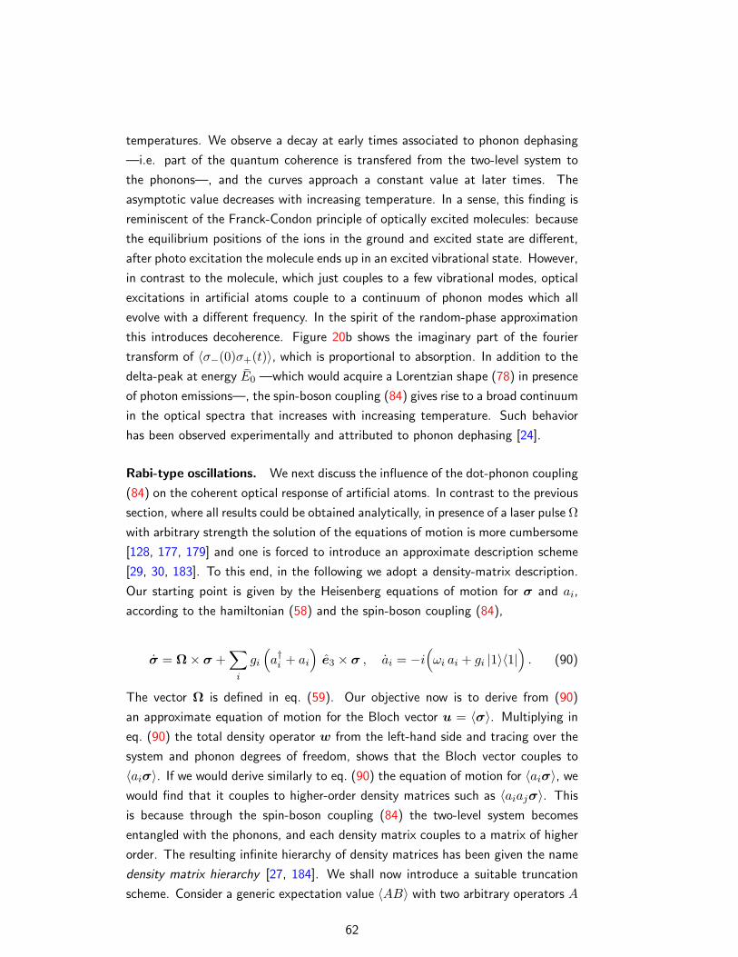
temperatures. We observe a decay at early times associated to phonon dephasing

—i.e. part of the quantum coherence is transfered from the two-level system to

the phonons—, and the curves approach a constant value at later times. The

asymptotic value decreases with increasing temperature. In a sense, this finding is

reminiscent of the Franck-Condon principle of optically excited molecules: because

the equilibrium positions of the ions in the ground and excited state are different,

after photo excitation the molecule ends up in an excited vibrational state. However,

in contrast to the molecule, which just couples to a few vibrational modes, optical

excitations in artificial atoms couple to a continuum of phonon modes which all

evolve with a different frequency. In the spirit of the random-phase approximation

this introduces decoherence. Figure 20b shows the imaginary part of the fourier

transform of 〈σ−(0)σ+(t)〉, which is proportional to absorption. In addition to the

delta-peak at energy E0 —which would acquire a Lorentzian shape (78) in presence

of photon emissions—, the spin-boson coupling (84) gives rise to a broad continuum

in the optical spectra that increases with increasing temperature. Such behavior

has been observed experimentally and attributed to phonon dephasing [24].

Rabi-type oscillations. We next discuss the influence of the dot-phonon coupling

(84) on the coherent optical response of artificial atoms. In contrast to the previous

section, where all results could be obtained analytically, in presence of a laser pulse Ωwith arbitrary strength the solution of the equations of motion is more cumbersome

[128, 177, 179] and one is forced to introduce an approximate description scheme

[29, 30, 183]. To this end, in the following we adopt a density-matrix description.

Our starting point is given by the Heisenberg equations of motion for σ and ai,

according to the hamiltonian (58) and the spin-boson coupling (84),

σ = Ω× σ +∑

i

gi

(a†i + ai

)e3 × σ , ai = −i

(ωi ai + gi |1〉〈1|

). (90)

The vector Ω is defined in eq. (59). Our objective now is to derive from (90)

an approximate equation of motion for the Bloch vector u = 〈σ〉. Multiplying in

eq. (90) the total density operator w from the left-hand side and tracing over the

system and phonon degrees of freedom, shows that the Bloch vector couples to

〈aiσ〉. If we would derive similarly to eq. (90) the equation of motion for 〈aiσ〉, we

would find that it couples to higher-order density matrices such as 〈aiajσ〉. This

is because through the spin-boson coupling (84) the two-level system becomes

entangled with the phonons, and each density matrix couples to a matrix of higher

order. The resulting infinite hierarchy of density matrices has been given the name

density matrix hierarchy [27, 184]. We shall now introduce a suitable truncation

scheme. Consider a generic expectation value 〈AB〉 with two arbitrary operators A

62

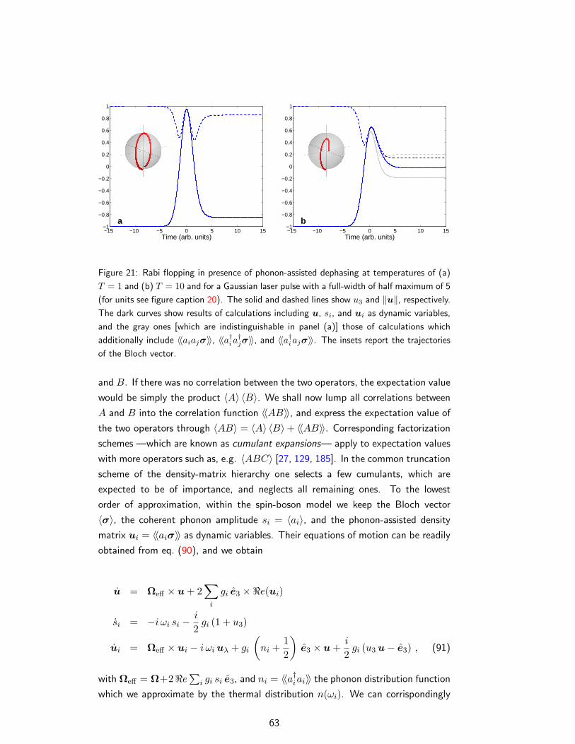
−15 −10 −5 0 5 10 15−1

−0.8

−0.6

−0.4

−0.2

0

0.2

0.4

0.6

0.8

1

a

Time (arb. units)−15 −10 −5 0 5 10 15−1

−0.8

−0.6

−0.4

−0.2

0

0.2

0.4

0.6

0.8

1

b

Time (arb. units)

Figure 21: Rabi flopping in presence of phonon-assisted dephasing at temperatures of (a)

T = 1 and (b) T = 10 and for a Gaussian laser pulse with a full-width of half maximum of 5

(for units see figure caption 20). The solid and dashed lines show u3 and ‖u‖, respectively.

The dark curves show results of calculations including u, si, and ui as dynamic variables,

and the gray ones [which are indistinguishable in panel (a)] those of calculations which

additionally include 〈〈aiajσ〉〉, 〈〈a†ia†jσ〉〉, and 〈〈a†iajσ〉〉. The insets report the trajectories

of the Bloch vector.

and B. If there was no correlation between the two operators, the expectation value

would be simply the product 〈A〉 〈B〉. We shall now lump all correlations between

A and B into the correlation function 〈〈AB〉〉, and express the expectation value of

the two operators through 〈AB〉 = 〈A〉 〈B〉+ 〈〈AB〉〉. Corresponding factorization

schemes —which are known as cumulant expansions— apply to expectation values

with more operators such as, e.g. 〈ABC〉 [27, 129, 185]. In the common truncation

scheme of the density-matrix hierarchy one selects a few cumulants, which are

expected to be of importance, and neglects all remaining ones. To the lowest

order of approximation, within the spin-boson model we keep the Bloch vector

〈σ〉, the coherent phonon amplitude si = 〈ai〉, and the phonon-assisted density

matrix ui = 〈〈aiσ〉〉 as dynamic variables. Their equations of motion can be readily

obtained from eq. (90), and we obtain

u = Ωeff × u+ 2∑

i

gi e3 ×<e(ui)

si = −i ωi si −i

2gi (1 + u3)

ui = Ωeff × ui − i ωi uλ + gi

(ni +

12

)e3 × u+

i

2gi (u3 u− e3) , (91)

with Ωeff = Ω+2<e∑

i gi si e3, and ni = 〈〈a†iai〉〉 the phonon distribution function

which we approximate by the thermal distribution n(ωi). We can corrispondingly

63

keep higher-order cumulants such as 〈〈a†iajσ〉〉 whose equations of motion are con-

siderably more complicated [29, 30]. On general grounds, we expect that the neglect

of higher-order cumulants is appropriate for sufficiently low temperatures and weak

dot-phonon couplings gi —or equivalently αp defined in eq. (89)—, which is a

valid assumption for GaAs-based quantum dots (αp∼= 0.033) at low temperatures.

Figure 21 shows results of calculations based on eq. (91) for a 2π-pulse and for

temperatures of T = 1 and T = 10. We observe that Rabi flopping occurs but is

damped because of the phonon-assisted dephasing. In particular at higher temper-

atures phonon dephasing is of strong importance, and gives rise to decoherence on

a picosecond time scale. We shall return to this point in section 6.

Beyond the spin-boson model. Although in many cases of interest the spin-

boson model (84) provides a sufficiently sophisticated description of optical exci-

tations in artificial atoms, there are situations where it is expected to break down.

For instance, at higher temperatures anharmonic decay of phonons —a phonon

decays in an energy-conserving scattering into two phonons of lower energy— or

higher-order phonon processes [186] could play a decisive role. If the artificial atom

can no longer be described as a genuine two-level system, one has to additionally

consider phonon-mediated scattering channels. Quite generally, the strong polar-

optical coupling to longitudinal optical phonons introduces a marked deformation

of the surrounding lattice and the formation of a polaron [187, 188, 189]. Because

optical phonons have a very small dispersion, this interaction channel has no sig-

nificant impact on decoherence. However, when the system is in an excited exciton

or multi-exciton state, the anharmonic decay of phonons contributing to the po-

laron allows for relaxation processes even in absence of energy matching between

the unrenormalized dot transition and the phonons [180, 190, 191, 192, 193, 194].

This demonstrates that phonon relaxation and decoherence in artificial atoms is

more efficient than one would expect in a simple-minded Fermi’s-golden-rule pic-

ture. Future work will show to what extent carrier-phonon interactions can be

tailored in artificial atoms [195, 196], and whether phonon-assisted dephasing can

be eventually strongly suppressed or fully overcome [183, 197, 198].

5.6 Spin scatterings

So far we have seen that photon and phonon scatterings occur on a timescale rang-

ing from several tens of picoseconds to nanoseconds. Such decoherence times are

remarkably long for the solid state, but are rather short when it comes to more

sophisticated quantum control applications (secs. 6 and 7). Optical excitations in

quantum dots possess another degree of freedom which has recently attracted enor-

mous interest: spin [53]. Spin couples weakly to the solid state environment, and is

64

therefore expected to be long lived. Optics provides a simple means to modify spin

degrees of freedom through coupling to the charge degrees. This dual nature of

optical excitations is exploited in quantum-computation proposals, to be discussed

in sec. 7. What are the typical spin relaxation and decoherence times in artificial

atoms? Things are quite unclear. Experimentally, it was found that at low temper-

ature spin relaxation is almost completely quenched [34, 35, 199, 200]. Theoretical

estimates indicate relaxation times of the order of microseconds or above [201],

whereas almost no conclusive results exist for the pertinent decoherence times.

Thus, spin keeps its secret in the game and holds a lot of promise and hope.

6 Quantum control

Recent years have witnessed enormous interest in controlling quantum phenomena

in a variety of nanoscale systems [202]. Quite generally, such control allows to

modify the system’s wavefunction at will through appropriate tailoring of external

fields, e.g., laser pulses: while in quantum optics the primary interest of this wave-

function engineering lies on the exploitation of quantum coherence among a few

atomic levels [15, 22, 89], in quantum chemistry optical control of molecular states

has even led to the demonstration of optically driven chemical reactions of com-

plex molecules [203]; furthermore, starting with the seminal work of Heberle et al.

[204] coherent-carrier control in semiconductors and semiconductor nanostructures

has been established as a mature field of research on its own. This research are-

nas have recently received further impetus from the emerging fields of quantum

computation and quantum communication [19], aiming at quantum devices where

the wavefunction can be manipulated with highest possible precision. It is worth

emphasizing that hitherto there exists no clear consensus of how to optimally tailor

the system’s control, and it appears that each field of research has come up with

its own strategies: for instance, quantum-optical implementations in atoms benefit

from the long atomic coherence times of meta-stable states, and it usually suffices

to rely on the solutions of effective models (e.g., adiabatic population transfer in an

effective three-level system [205]); in contrast, in quantum chemistry the complexity

of molecular states usually does not permit schemes which are solely backed from

the underlying level schemes, and learning algorithms, which receive direct feed-

back from experiment, appear to be the method of choice. Finally, coherent control

in semiconductor nanostructures has hitherto been primarily inspired by quantum-

optical techniques; however, it is clear that control in future quantum devices will

require more sophisticated techniques to account for the enhanced decoherence in

the solid state.

This section is devoted to an introduction into the field. Throughout we shall

65

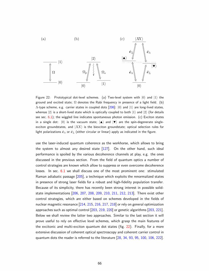
|0〉

|1〉

Ω

(a)

KS

|0〉 |1〉

|2〉

Ωp Ωs

(b)

HP

NV&&&&&&&&&

&&&&&&&&& OOOOO

|0〉

|N〉

|H〉

|XX〉

eλ eλ

eλ eλ

(c)

NV%%%%%%%%%%%

%%%%%%%%%%%

HP

HP

NV

%%%%%%%%%%%

%%%%%%%%%%%

Figure 22: Prototypical dot-level schemes. (a) Two-level system with |0〉 and |1〉 the

ground and excited state; Ω denotes the Rabi frequency in presence of a light field. (b)

Λ-type scheme, e.g. carrier states in coupled dots [206]: |0〉 and |1〉 are long-lived states,

whereas |2〉 is a short-lived state which is optically coupled to both |1〉 and |2〉 (for details

see sec. 6.1); the wiggled line indicates spontaneous photon emission. (c) Exciton states

in a single dot: |0〉 is the vacuum state; |N〉 and |H〉 are the spin-degenerate single-

exciton groundstates, and |XX〉 is the biexciton groundstate; optical selection rules for

light polarizations eλ or eλ (either circular or linear) apply as indicated in the figure.

use the laser-induced quantum coherence as the workhorse, which allows to bring

the system to almost any desired state [127]. On the other hand, such ideal

performance is spoiled by the various decoherence channels at play, e.g. the ones

discussed in the previous section. From the field of quantum optics a number of

control strategies are known which allow to suppress or even overcome decoherence

losses. In sec. 6.1 we shall discuss one of the most prominent one: stimulated

Raman adiabatic passage [205], a technique which exploits the renormalized states

in presence of strong laser fields for a robust and high-fidelity population transfer.

Because of its simplicity, there has recently been strong interest in possible solid-

state implementations [206, 207, 208, 209, 210, 211, 212, 213]. There exist other

control strategies, which are either based on schemes developed in the fields of

nuclear magnetic resonance [214, 215, 216, 217, 218] or rely on general optimization

approaches such as optimal control [203, 219, 220] or genetic algorithms [203, 221].

Below we shall review the latter two approaches. Similar to the last section it will

prove useful to rely on effective level schemes, which grasp the main features of

the excitonic and multi-exciton quantum dot states (fig. 22). Finally, for a more

extensive discussion of coherent optical spectroscopy and coherent carrier control in

quantum dots the reader is referred to the literature [28, 34, 93, 95, 100, 106, 222].

66

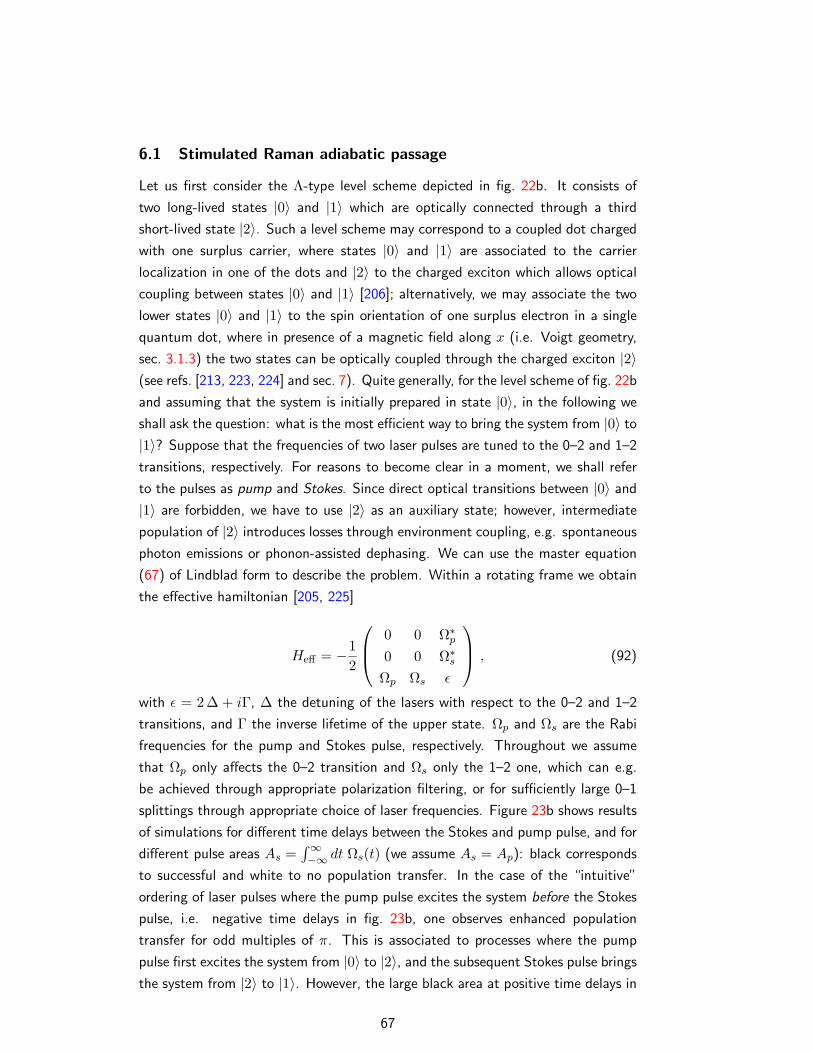
6.1 Stimulated Raman adiabatic passage

Let us first consider the Λ-type level scheme depicted in fig. 22b. It consists of

two long-lived states |0〉 and |1〉 which are optically connected through a third

short-lived state |2〉. Such a level scheme may correspond to a coupled dot charged

with one surplus carrier, where states |0〉 and |1〉 are associated to the carrier

localization in one of the dots and |2〉 to the charged exciton which allows optical

coupling between states |0〉 and |1〉 [206]; alternatively, we may associate the two

lower states |0〉 and |1〉 to the spin orientation of one surplus electron in a single

quantum dot, where in presence of a magnetic field along x (i.e. Voigt geometry,

sec. 3.1.3) the two states can be optically coupled through the charged exciton |2〉(see refs. [213, 223, 224] and sec. 7). Quite generally, for the level scheme of fig. 22b

and assuming that the system is initially prepared in state |0〉, in the following we

shall ask the question: what is the most efficient way to bring the system from |0〉 to

|1〉? Suppose that the frequencies of two laser pulses are tuned to the 0–2 and 1–2

transitions, respectively. For reasons to become clear in a moment, we shall refer

to the pulses as pump and Stokes. Since direct optical transitions between |0〉 and

|1〉 are forbidden, we have to use |2〉 as an auxiliary state; however, intermediate

population of |2〉 introduces losses through environment coupling, e.g. spontaneous

photon emissions or phonon-assisted dephasing. We can use the master equation

(67) of Lindblad form to describe the problem. Within a rotating frame we obtain

the effective hamiltonian [205, 225]

Heff = −12

0 0 Ω∗p

0 0 Ω∗s

Ωp Ωs ε

, (92)

with ε = 2 ∆ + iΓ, ∆ the detuning of the lasers with respect to the 0–2 and 1–2

transitions, and Γ the inverse lifetime of the upper state. Ωp and Ωs are the Rabi

frequencies for the pump and Stokes pulse, respectively. Throughout we assume

that Ωp only affects the 0–2 transition and Ωs only the 1–2 one, which can e.g.

be achieved through appropriate polarization filtering, or for sufficiently large 0–1

splittings through appropriate choice of laser frequencies. Figure 23b shows results

of simulations for different time delays between the Stokes and pump pulse, and for

different pulse areas As =∫∞−∞ dt Ωs(t) (we assume As = Ap): black corresponds

to successful and white to no population transfer. In the case of the “intuitive”

ordering of laser pulses where the pump pulse excites the system before the Stokes

pulse, i.e. negative time delays in fig. 23b, one observes enhanced population

transfer for odd multiples of π. This is associated to processes where the pump

pulse first excites the system from |0〉 to |2〉, and the subsequent Stokes pulse brings

the system from |2〉 to |1〉. However, the large black area at positive time delays in

67

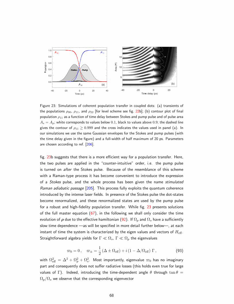
Figure 23: Simulations of coherent population transfer in coupled dots: (a) transients of

the populations ρ00, ρ11, and ρ22 [for level scheme see fig. 22b]; (b) contour plot of final

population ρ11 as a function of time delay between Stokes and pump pulse and of pulse area

As = Ap; white corresponds to values below 0.1, black to values above 0.9; the dashed line

gives the contour of ρ11 ≥ 0.999 and the cross indicates the values used in panel (a). In

our simulations we use the same Gaussian envelopes for the Stokes and pump pulses (with

the time delay given in the figure) and a full-width of half maximum of 20 ps. Parameters

are chosen according to ref. [206].

fig. 23b suggests that there is a more efficient way for a population transfer. Here,

the two pulses are applied in the “counter-intuitive” order, i.e. the pump pulse

is turned on after the Stokes pulse. Because of the resemblance of this scheme

with a Raman-type process it has become convenient to introduce the expression

of a Stokes pulse, and the whole process has been given the name stimulated

Raman adiabatic passage [205]. This process fully exploits the quantum coherence

introduced by the intense laser fields. In presence of the Stokes pulse the dot-states

become renormalized, and these renormalized states are used by the pump pulse

for a robust and high-fidelity population transfer. While fig. 23 presents solutions

of the full master equation (67), in the following we shall only consider the time

evolution of ρ due to the effective hamiltonian (92). If Ωp and Ωs have a sufficiently

slow time dependence —as will be specified in more detail further below—, at each

instant of time the system is characterized by the eigen values and vectors of Heff .

Straightforward algebra yields for Γ Ωs, Γ Ωp the eigenvalues

$0 = 0 , $± =12

(∆± Ωeff) + i (1−∆/Ωeff) Γ , (93)

with Ω2eff = ∆2 + Ω2

p + Ω2s. Most importantly, eigenvalue $0 has no imaginary

part and consequently does not suffer radiative losses (this holds even true for large

values of Γ). Indeed, introducing the time-dependent angle θ through tan θ =Ωp/Ωs we observe that the corresponding eigenvector

68

|a0〉 = cos θ|0〉 − sin θ|1〉 (94)

has no component of the “leaky” state |2〉 — in contrast to the eigenvectors |a±〉which are composed of all three states |0〉, |1〉, and |2〉. In |a0〉 the amplitudes of

the 0–2 and 1–2 transitions interfere destructively, such that the state is completely

stable against absorption and emission from the radiation fields. For that reason

state |a0〉 has been given the name trapped state. The population transfer process

exploits this trapped state as a vehicle in order to transfer population between states

|0〉 and |1〉. It is achieved by using overlap in time between the two laser pulses

(fig. 23a, table 5). Initially, the system is prepared in state |0〉. When the first

(Stokes) laser is smoothly turned on, the system is excited at the Stokes frequency.

At this frequency no transitions can be induced; what the pulse does, however, is

to align the time-dependent state vector |Ψ(t)〉 with |a0(t)〉 = |0〉 (since θ = 0 in

the sector Ωs 6= 0, Ωp = 0), and to split the degeneracy of the eigenvalues $0

and $±. Thus, if the pump laser is smoothly turned on —such that throughout

Ωeff(t) remains large enough to avoid non-adiabatic transitions between |a0(t)〉 and

|a±(t)〉 [205]— all population is transferred between states |0〉 and |1〉 within an

adiabatic process where |Ψ(t)〉 directly follows the time-dependent trapped state

|a0(t)〉. Stimulated Raman adiabatic passage is a process important for a number

of reasons. First, it is a prototypical example of how intense laser fields can cause

drastic renormalizations of carrier states; quite generally, these “dressed” states

exhibit novel features in case of quantum interference, i.e. if three or more states

are optically coupled. Second, quantum control in quantum dots has recently

attracted increasing interest in view of possible quantum computation applications

[213, 216, 226, 227] aiming at an all-optical control of carrier states; in this respect,

the adiabatic transfer scheme might be of some importance because of its robustness

and its high fidelity (sec. 7). More specifically, from fig. 23b it becomes apparent

that the transfer works successfully within a relatively large parameter regime — in

contrast to the “intuitive” order of pulses, where a detailed knowledge of the dipole

matrix elements and a precise control over the laser parameters is required. Thus,

Table 5: Time evolution of the quantities characterizing the stimulated Raman adiabatic

passage [205]. For discussion see text.

Quantity Ωs on Ωs and Ωp on Ωp on

Angle θ 0 0 → π/2 π/2∼ $± −∆/2 ± 1

2 (∆2 + Ω2s)

12 ± 1

2 (∆2 + Ω2s + Ω2

p)12 ± 1

2 (∆2 + Ω2p)

12

$0 0 0 0

Trapped state |a0〉 |0〉 |0〉 → |1〉 |1〉

69

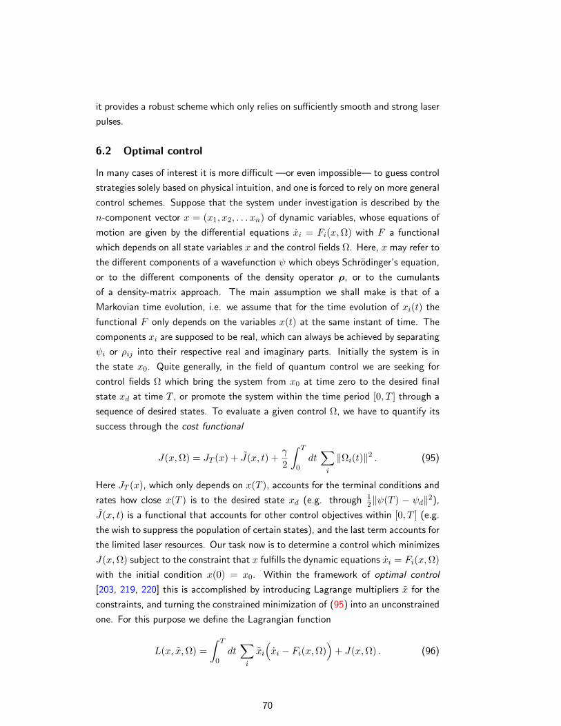
it provides a robust scheme which only relies on sufficiently smooth and strong laser

pulses.

6.2 Optimal control

In many cases of interest it is more difficult —or even impossible— to guess control

strategies solely based on physical intuition, and one is forced to rely on more general

control schemes. Suppose that the system under investigation is described by the

n-component vector x = (x1, x2, . . . xn) of dynamic variables, whose equations of

motion are given by the differential equations xi = Fi(x,Ω) with F a functional

which depends on all state variables x and the control fields Ω. Here, x may refer to

the different components of a wavefunction ψ which obeys Schrodinger’s equation,

or to the different components of the density operator ρ, or to the cumulants

of a density-matrix approach. The main assumption we shall make is that of a

Markovian time evolution, i.e. we assume that for the time evolution of xi(t) the

functional F only depends on the variables x(t) at the same instant of time. The

components xi are supposed to be real, which can always be achieved by separating

ψi or ρij into their respective real and imaginary parts. Initially the system is in

the state x0. Quite generally, in the field of quantum control we are seeking for

control fields Ω which bring the system from x0 at time zero to the desired final

state xd at time T , or promote the system within the time period [0, T ] through a

sequence of desired states. To evaluate a given control Ω, we have to quantify its

success through the cost functional

J(x,Ω) = JT (x) + J(x, t) +γ

2

∫ T

0dt∑

i

‖Ωi(t)‖2 . (95)

Here JT (x), which only depends on x(T ), accounts for the terminal conditions and

rates how close x(T ) is to the desired state xd (e.g. through 12‖ψ(T ) − ψd‖2),

J(x, t) is a functional that accounts for other control objectives within [0, T ] (e.g.

the wish to suppress the population of certain states), and the last term accounts for

the limited laser resources. Our task now is to determine a control which minimizes

J(x,Ω) subject to the constraint that x fulfills the dynamic equations xi = Fi(x,Ω)with the initial condition x(0) = x0. Within the framework of optimal control

[203, 219, 220] this is accomplished by introducing Lagrange multipliers x for the

constraints, and turning the constrained minimization of (95) into an unconstrained

one. For this purpose we define the Lagrangian function

L(x, x,Ω) =∫ T

0dt∑

i

xi

(xi − Fi(x,Ω)

)+ J(x,Ω) . (96)

70

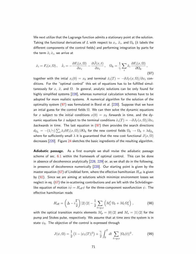
We next utilize that the Lagrange function admits a stationary point at the solution.

Taking the functional derivatives of L with respect to xi, xi, and Ωk (k labels the

different components of the control fields) and performing integration by parts for

the term xi xi, we arrive at

xi = Fi(x,Ω) , ˙xi = −∂Fi(x,Ω)∂xi

− ∂J(x, t)∂xi

, Ωk =1γ

∑i

xi∂Fi(x,Ω)∂Ωk

,

(97)

together with the intial xi(0) = x0 and terminal xi(T ) = −∂JT (x,Ω)/∂xi con-

ditions. For the “optimal control” this set of equations has to be fulfilled simul-

taneously for x, x, and Ω. In general, analytic solutions can be only found for

highly simplified systems [228], whereas numerical calculation schemes have to be

adopted for more realistic systems. A numerical algorithm for the solution of the

optimality system (97) was formulated in Borzı et al. [220]. Suppose that we have

an intial guess for the control fields Ω. We can then solve the dynamic equations

for x subject to the initial conditions x(0) = x0 forwards in time, and the dy-

namic equations for x subject to the terminal conditions xi(T ) = −∂JT (x,Ω)/∂xi

backwards in time. The last equation in (97) then provides the search directions

dΩk= −(1/γ)

∑i xi∂Fi(x,Ω)/∂Ωk for the new control fields Ωk → Ωk + λdΩk

where for sufficiently small λ it is guaranteed that the new cost functional J(x,Ω)decreases [220]. Figure 24 sketches the basic ingredients of the resulting algorithm.

Adiabatic passage. As a first example we shall revise the adiabatic passage

scheme of sec. 6.1 within the framework of optimal control. This can be done

in absence of decoherence analytically [228, 229] or, as we shall do in the following,

in presence of decoherence numerically [220]. Our starting point is given by the

master equation (67) of Lindblad form, where the effective hamiltonian Heff is given

by (92). Since we are aiming at solutions which minimize environment losses we

neglect in eq. (67) the in-scattering contributions and are left with the Schrodinger-

like equation of motion iψ = Heffψ for the three-component wavefunction ψ. The

effective hamiltonian reads

Heff =(

∆− iΓ2

)|2〉〈2| − 1

2

∑`=p,s

(M †

` Ω` +M` Ω∗`

), (98)

with the optical transition matrix elements Mp = |0〉〈2| and Ms = |1〉〈2| for the

pump and Stokes pulse, respectively. We assume that at time zero the system is in

state ψ0. The objective of the control is expressed through

J(ψ,Ω) =12(1− |ψ1(T )|2

)+γ

2

∫ T

0dt∑`=p,s

|Ω`(t)|2 . (99)

71

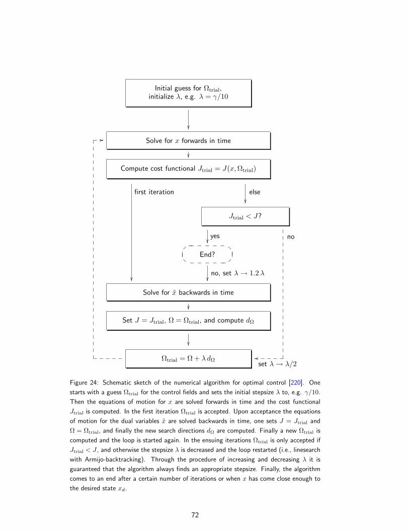
Initial guess for Ωtrial,initialize λ, e.g. λ = γ/10

Solve for x forwards in time

Compute cost functional Jtrial = J(x,Ωtrial)

Jtrial < J?

End?

_

_ _ _ _ _

? ?

_ _ _ _ __

Solve for x backwards in time

Set J = Jtrial, Ω = Ωtrial, and compute dΩ

Ωtrial = Ω + λ dΩ

first iteration else

yes no

no, set λ→ 1.2λ

set λ→ λ/2

_ _ _ _ _

oo_ _ _ _ _

//__

Figure 24: Schematic sketch of the numerical algorithm for optimal control [220]. One

starts with a guess Ωtrial for the control fields and sets the initial stepsize λ to, e.g. γ/10.

Then the equations of motion for x are solved forwards in time and the cost functional

Jtrial is computed. In the first iteration Ωtrial is accepted. Upon acceptance the equations

of motion for the dual variables x are solved backwards in time, one sets J = Jtrial and

Ω = Ωtrial, and finally the new search directions dΩ are computed. Finally a new Ωtrial is

computed and the loop is started again. In the ensuing iterations Ωtrial is only accepted if

Jtrial < J , and otherwise the stepsize λ is decreased and the loop restarted (i.e., linesearch

with Armijo-backtracking). Through the procedure of increasing and decreasing λ it is

guaranteed that the algorithm always finds an appropriate stepsize. Finally, the algorithm

comes to an end after a certain number of iterations or when x has come close enough to

the desired state xd.

72

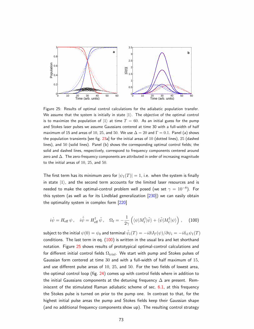
0 10 20 30 40 50 600

0.2

0.4

0.6

0.8

1

Time (arb. units)

Pop

ulat

ion

a

0 10 20 30 40 50 600

0.5

1

1.5

2

2.5

3

3.5

Time (arb. units)

|Ω(t

)|

b

Figure 25: Results of optimal control calculations for the adiabatic population transfer.

We assume that the system is initially in state |1〉. The objective of the optimal control

is to maximize the population of |1〉 at time T = 60. As an initial guess for the pump

and Stokes laser pulses we assume Gaussians centered at time 30 with a full-width of half

maximum of 15 and areas of 10, 25, and 50. We use ∆ = 20 and Γ = 0.1. Panel (a) shows

the population transients [see fig. 23a] for the initial areas of 10 (dotted lines), 25 (dashed

lines), and 50 (solid lines). Panel (b) shows the corresponding optimal control fields; the

solid and dashed lines, respectively, correspond to frequency components centered around

zero and ∆. The zero-frequency components are attributed in order of increasing magnitude

to the initial areas of 10, 25, and 50.

The first term has its minimum zero for |ψ1(T )| = 1, i.e. when the system is finally

in state |1〉, and the second term accounts for the limited laser resources and is

needed to make the optimal-control problem well posed (we set γ = 10−8). For

this system (as well as for its Lindblad generalization [230]) we can easily obtain

the optimality system in complex form [220]

iψ = Heff ψ , i˙ψ = H†

eff ψ , Ω` = − 12γ

(〈ψ|M †

` |ψ〉+ 〈ψ|M †` |ψ〉

), (100)

subject to the initial ψ(0) = ψ0 and terminal ψi(T ) = −i∂JT (ψ)/∂ψi = −iδi1ψ1(T )conditions. The last term in eq. (100) is written in the usual bra and ket shorthand

notation. Figure 25 shows results of prototypical optimal-control calculations and

for different initial control fields Ωtrial. We start with pump and Stokes pulses of

Gaussian form centered at time 30 and with a full-width of half maximum of 15,

and use different pulse areas of 10, 25, and 50. For the two fields of lowest area,

the optimal control loop (fig. 24) comes up with control fields where in addition to

the initial Gaussians components at the detuning frequency ∆ are present. Rem-

iniscent of the stimulated Raman adiabatic scheme of sec. 6.1, at this frequency

the Stokes pulse is turned on prior to the pump one. In contrast to that, for the

highest initial pulse areas the pump and Stokes fields keep their Gaussian shape

(and no additional frequency components show up). The resulting control strategy

73

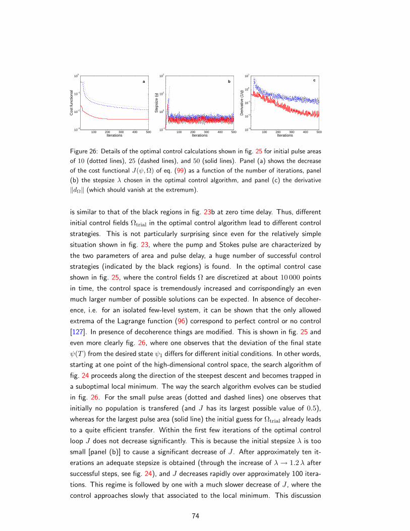
100 200 300 400 50010

−3

10−2

10−1

100

Iterations

Cos

t fun

ctio

nal

a

100 200 300 400 50010

−1

100

101

102

Iterations

Ste

psiz

e (γ

)

b

100 200 300 400 50010

−3

10−2

10−1

100

101

Iterations

Der

ivat

ive

(1/γ)

c

Figure 26: Details of the optimal control calculations shown in fig. 25 for initial pulse areas

of 10 (dotted lines), 25 (dashed lines), and 50 (solid lines). Panel (a) shows the decrease

of the cost functional J(ψ,Ω) of eq. (99) as a function of the number of iterations, panel

(b) the stepsize λ chosen in the optimal control algorithm, and panel (c) the derivative

‖dΩ‖ (which should vanish at the extremum).

is similar to that of the black regions in fig. 23b at zero time delay. Thus, different

initial control fields Ωtrial in the optimal control algorithm lead to different control

strategies. This is not particularly surprising since even for the relatively simple

situation shown in fig. 23, where the pump and Stokes pulse are characterized by

the two parameters of area and pulse delay, a huge number of successful control

strategies (indicated by the black regions) is found. In the optimal control case

shown in fig. 25, where the control fields Ω are discretized at about 10 000 points

in time, the control space is tremendously increased and corrispondingly an even

much larger number of possible solutions can be expected. In absence of decoher-

ence, i.e. for an isolated few-level system, it can be shown that the only allowed

extrema of the Lagrange function (96) correspond to perfect control or no control

[127]. In presence of decoherence things are modified. This is shown in fig. 25 and

even more clearly fig. 26, where one observes that the deviation of the final state

ψ(T ) from the desired state ψ1 differs for different initial conditions. In other words,

starting at one point of the high-dimensional control space, the search algorithm of

fig. 24 proceeds along the direction of the steepest descent and becomes trapped in

a suboptimal local minimum. The way the search algorithm evolves can be studied

in fig. 26. For the small pulse areas (dotted and dashed lines) one observes that

initially no population is transfered (and J has its largest possible value of 0.5),

whereas for the largest pulse area (solid line) the initial guess for Ωtrial already leads

to a quite efficient transfer. Within the first few iterations of the optimal control

loop J does not decrease significantly. This is because the initial stepsize λ is too

small [panel (b)] to cause a significant decrease of J . After approximately ten it-

erations an adequate stepsize is obtained (through the increase of λ→ 1.2λ after

successful steps, see fig. 24), and J decreases rapidly over approximately 100 itera-

tions. This regime is followed by one with a much slower decrease of J , where the

control approaches slowly that associated to the local minimum. This discussion

74

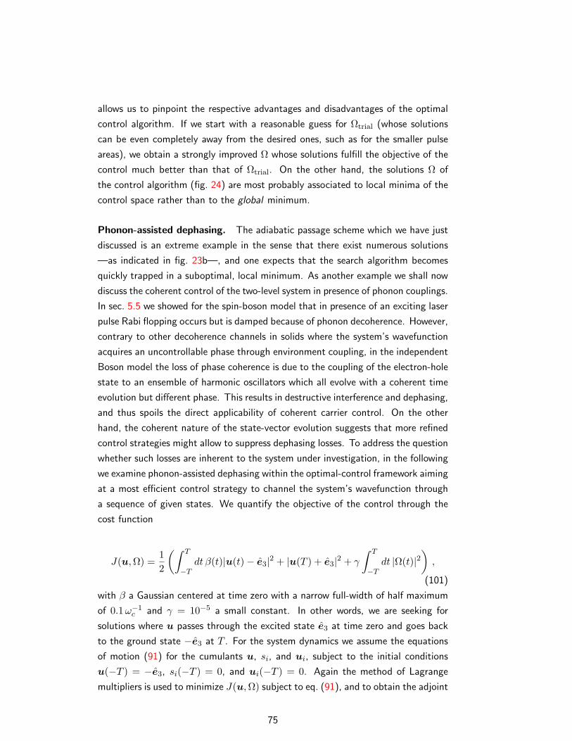
allows us to pinpoint the respective advantages and disadvantages of the optimal

control algorithm. If we start with a reasonable guess for Ωtrial (whose solutions

can be even completely away from the desired ones, such as for the smaller pulse

areas), we obtain a strongly improved Ω whose solutions fulfill the objective of the

control much better than that of Ωtrial. On the other hand, the solutions Ω of

the control algorithm (fig. 24) are most probably associated to local minima of the

control space rather than to the global minimum.

Phonon-assisted dephasing. The adiabatic passage scheme which we have just

discussed is an extreme example in the sense that there exist numerous solutions

—as indicated in fig. 23b—, and one expects that the search algorithm becomes

quickly trapped in a suboptimal, local minimum. As another example we shall now

discuss the coherent control of the two-level system in presence of phonon couplings.

In sec. 5.5 we showed for the spin-boson model that in presence of an exciting laser

pulse Rabi flopping occurs but is damped because of phonon decoherence. However,

contrary to other decoherence channels in solids where the system’s wavefunction

acquires an uncontrollable phase through environment coupling, in the independent

Boson model the loss of phase coherence is due to the coupling of the electron-hole

state to an ensemble of harmonic oscillators which all evolve with a coherent time

evolution but different phase. This results in destructive interference and dephasing,

and thus spoils the direct applicability of coherent carrier control. On the other

hand, the coherent nature of the state-vector evolution suggests that more refined

control strategies might allow to suppress dephasing losses. To address the question

whether such losses are inherent to the system under investigation, in the following

we examine phonon-assisted dephasing within the optimal-control framework aiming

at a most efficient control strategy to channel the system’s wavefunction through

a sequence of given states. We quantify the objective of the control through the

cost function

J(u,Ω) =12

(∫ T

−Tdt β(t)|u(t)− e3|2 + |u(T ) + e3|2 + γ

∫ T

−Tdt |Ω(t)|2

),

(101)

with β a Gaussian centered at time zero with a narrow full-width of half maximum

of 0.1ω−1c and γ = 10−5 a small constant. In other words, we are seeking for

solutions where u passes through the excited state e3 at time zero and goes back

to the ground state −e3 at T . For the system dynamics we assume the equations

of motion (91) for the cumulants u, si, and ui, subject to the initial conditions

u(−T ) = −e3, si(−T ) = 0, and ui(−T ) = 0. Again the method of Lagrange

multipliers is used to minimize J(u,Ω) subject to eq. (91), and to obtain the adjoint

75

−15 −10 −5 0 5 10 150

0.2

0.4

0.6

0.8

1

1.2

1.4

1.6

Time ( 1/ωc )

Con

trol

( ω

c )

(a)GaussOptimal

−15 −10 −5 0 5 10 15−1

−0.8

−0.6

−0.4

−0.2

0

0.2

0.4

0.6

0.8

1

Time ( 1/ωc )

u 3( t )

(b)

Figure 27: Results of our calculations with a Gaussian 2π (dashed lines) and optimal-

control (solid lines) laser pulse and for zero temperature and an electron-phonon coupling

of αp = 0.1. Panel (a) shows |Ω(t)| and panel (b) the time evolution of u3(t), and the insets

the trajectories of the Bloch vector u(t). For the Gaussian 2π-pulse Rabi flopping occurs

but is damped due to electron-phonon interactions. For the optimal control decoherence

losses are completely suppressed, and the the system passes through the desired states of

e3 at time zero and −e3 at T .

equations [183]

˙u = Ω× u+∑

i

gi

((ni +

12)e3 ×<e(ui) +

12=m

((si − u ui) e3 − u3 ui

))+β(t)(u− e3)

˙si = −iωisi + 2 gi

((u× u) e3 + <e

∑j

(u∗j × uj) e3

)˙ui = Ω× ui − iωiui + 2 gi e3 × u , (102)

with terminal conditions u(T ) = −e3 − u(T ), si(T ) = 0, and ui(T ) = 0. Equa-

tions (91) and (102) together with

Ω =1γ

((u× u) + <e

∑i

(u∗i × ui)

)(e1 − ie2) (103)

form the optimality system. It is solved iteratively through the scheme depicted in

fig. 24, with integration of eq. (91) forwards and eq. (102) backwards in time, and

computing an improved control by use of eq. (103). Results of such optimal-control

calculations are shown in fig. 27. Most remarkably, one can indeed obtain a control

field for which u(t) passes through the desired states of e3 at time zero and −e3

at T . Thus, appropriate pulse shaping allows to fully control the two-level system

even in presence of phonon couplings. We emphasize that, with the exception of

the somewhat pathological quantum “bang-bang” control [128] where the system

76

is constantly flipped to suppress decoherence, no such simple control strategy for

suppression of environment losses is known in the literature. This result, which

also prevails in presence of finite but low termperatures [183], clearly highlights the

strength and flexibility of optimal control.

Genetic algorithms. In several cases of interest one is often neither able to solve

the equations of motion nor knows the full hamiltonian characterizing the system.

This holds in particular true for laser-induced reactions of molecules [203], where the

configuration landscape is highly complicated. Judson and Rabitz [231] were the

first to propose an evolutionary algorithm that allows the search for control fields

even without any knowledge of the hamiltonian. For the sake of completeness, in the

following we shall briefly outline the main ideas of this approach. Suppose that the

laser pulse can be encoded in terms of a “gene”, i.e. a vector Ω = (Ω1,Ω2, . . .Ωn)with typically n ∼ 10–100 components. Within the evolutionary approach a popu-

lation Npop∼= 48 of different genes Ωµ is considered. At the beginning the different

components of each gene are chosen randomly. Next, we compute for each gene

the objective function Jµ. Within the evolutionary approach, the next popula-

tion of genes is determined in biological terms according to the fitness Jµ of each

individual [221, 231]. Following Zeidler et al. [221] this can be accomplished as

follows: first, the individual with the best Jµ is included without change in the

next generation (elitism); next, the Nparent ∼ Npop/7 individuals with the best Jµ

are chosen as parents for the next generation; about 2Nparent of the individuals

of the next generation are determined by randomly choosing two parents, cutting

their genes at one given point (single-point crossover) or two points (two-point

crossover), and pasting the different pieces of the genes together (recombination);

finally, the remaining individuals of the next generation are obtained by randomly

taking one parent and randomly modifying its genetic information Ωµi (mutation).

There exist numerous other implementations which differ in one or several points.

However, the grand idea of all these approaches is to provide a sufficiently large

gene pool and to let the individuals benefit from their respective advantages and

peculiarities. This has the consequence that once an individual acquires a successful

control strategy (either through recombination or mutation), it will distribute it to

the next generation where it possibly becomes optimized through further mixing or

mutation. For that it is compulsory to keep not only the fittest individual but to

provide a larger gene pool. In this respect, mutation plays an important role as it

determines the degree of modification from one generation to the next. For nor-

malized control-field components Ωµi ∈ [0, 1] mutation can be computed according

to [221, 232]

77

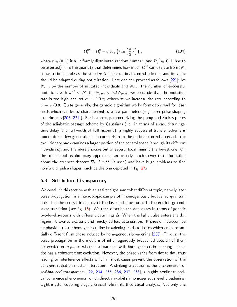
Ωµi′ = Ωµ

i − σ log(tan

(π2r))

, (104)

where r ∈ (0, 1) is a uniformly distributed random number (and Ωµi′ ∈ [0, 1] has to

be asserted). σ is the quantity that determines how much Ωµ′ can deviate from Ωµ.

It has a similar role as the stepsize λ in the optimal control scheme, and its value

should be adapted during optimization. Here one can proceed as follows [221]: let

Nmut be the number of mutated individuals and Nsucc the number of successful

mutations with Jµ′ < Jµ; for Nsucc < 0.2Nperm we conclude that the mutation

rate is too high and set σ → 0.9σ; otherwise we increase the rate according to

σ → σ/0.9. Quite generally, the genetic algorithm works formidably well for laser

fields which can be by characterized by a few parameters (e.g. laser-pulse shaping

experiments [203, 221]). For instance, parameterizing the pump and Stokes pulses

of the adiabatic passage scheme by Gaussians (i.e. in terms of areas, detunings,

time delay, and full-width of half maxima), a highly successful transfer scheme is

found after a few generations. In comparison to the optimal control approach, the

evolutionary one examines a larger portion of the control space (through its different

individuals), and therefore chooses out of several local minima the lowest one. On

the other hand, evolutionary approaches are usually much slower (no information

about the steepest descent ∇Ω J(x,Ω) is used) and have huge problems to find

non-trivial pulse shapes, such as the one depicted in fig. 27a.

6.3 Self-induced transparency

We conclude this section with an at first sight somewhat different topic, namely laser

pulse propagation in a macroscopic sample of inhomogenously broadened quantum

dots. Let the central frequency of the laser pulse be tuned to the exciton ground-

state transition (see fig. 13). We then describe the dot states in terms of generic

two-level systems with different detunings ∆. When the light pulse enters the dot

region, it excites excitons and hereby suffers attenuation. It should, however, be

emphasized that inhomogeneous line broadening leads to losses which are substan-

tially different from those induced by homogeneous broadening [233]. Through the

pulse propagation in the medium of inhomogenously broadened dots all of them

are excited in in phase, where —at variance with homogeneous broadening— each

dot has a coherent time evolution. However, the phase varies from dot to dot, thus

leading to interference effects which in most cases prevent the observation of the

coherent radiation-matter interaction. A striking exception is the phenomenon of

self-induced transparency [22, 234, 235, 236, 237, 238], a highly nonlinear opti-

cal coherence phenomenon which directly exploits inhomogeneous level broadening.

Light-matter coupling plays a crucial role in its theoretical analysis. Not only one

78

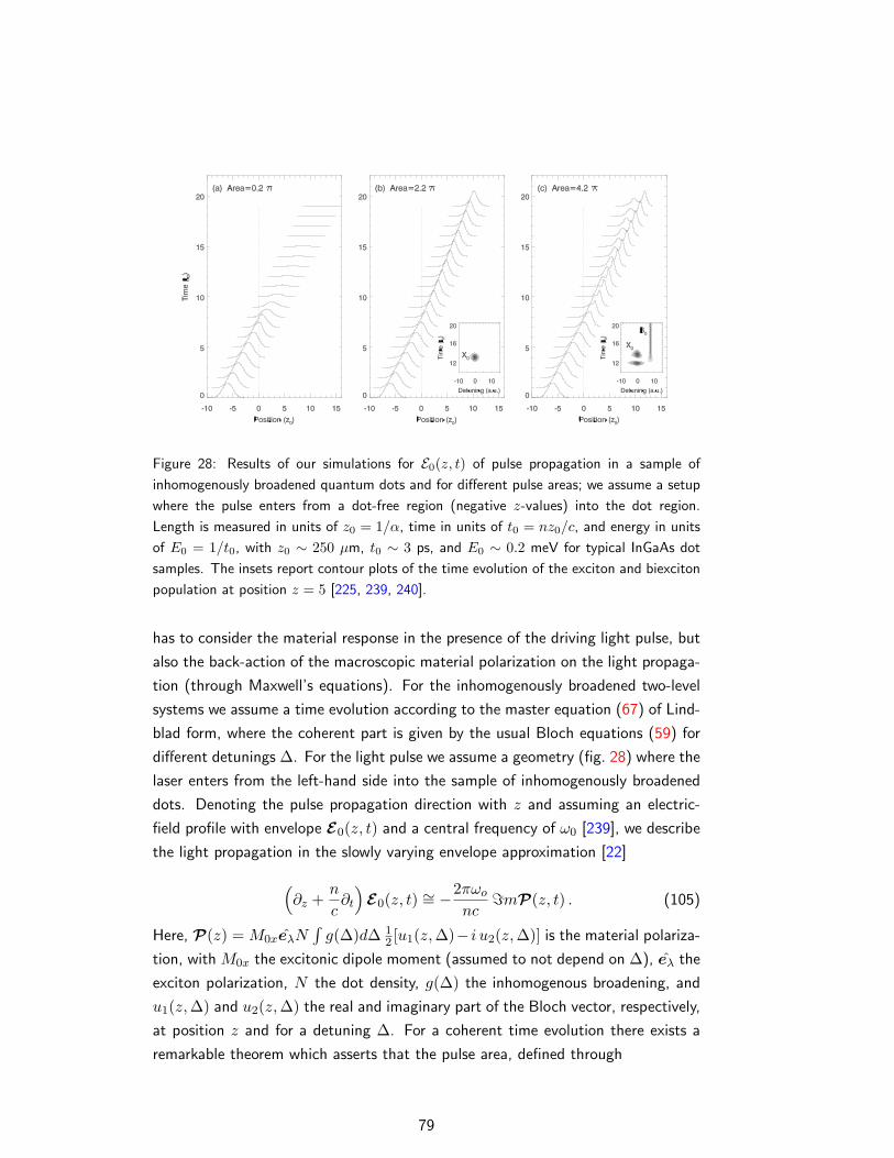
Figure 28: Results of our simulations for E0(z, t) of pulse propagation in a sample of

inhomogenously broadened quantum dots and for different pulse areas; we assume a setup

where the pulse enters from a dot-free region (negative z-values) into the dot region.

Length is measured in units of z0 = 1/α, time in units of t0 = nz0/c, and energy in units

of E0 = 1/t0, with z0 ∼ 250 µm, t0 ∼ 3 ps, and E0 ∼ 0.2 meV for typical InGaAs dot

samples. The insets report contour plots of the time evolution of the exciton and biexciton

population at position z = 5 [225, 239, 240].

has to consider the material response in the presence of the driving light pulse, but

also the back-action of the macroscopic material polarization on the light propaga-

tion (through Maxwell’s equations). For the inhomogenously broadened two-level

systems we assume a time evolution according to the master equation (67) of Lind-

blad form, where the coherent part is given by the usual Bloch equations (59) for

different detunings ∆. For the light pulse we assume a geometry (fig. 28) where the

laser enters from the left-hand side into the sample of inhomogenously broadened

dots. Denoting the pulse propagation direction with z and assuming an electric-

field profile with envelope E0(z, t) and a central frequency of ω0 [239], we describe

the light propagation in the slowly varying envelope approximation [22]

(∂z +

n

c∂t

)E0(z, t) ∼= −2πωo

nc=mP(z, t) . (105)

Here, P(z) = M0xeλN∫g(∆)d∆ 1

2 [u1(z,∆)− i u2(z,∆)] is the material polariza-

tion, with M0x the excitonic dipole moment (assumed to not depend on ∆), eλ the

exciton polarization, N the dot density, g(∆) the inhomogenous broadening, and

u1(z,∆) and u2(z,∆) the real and imaginary part of the Bloch vector, respectively,

at position z and for a detuning ∆. For a coherent time evolution there exists a

remarkable theorem which asserts that the pulse area, defined through

79

A(z) = M0x limt→∞

∫ t

−∞dt′ e∗λ ,E(z, t′) (106)

satisfies the equation [22, 235]

dA(z)dz

= −α2

sinA(z) , α =2π2Nω0M

20x

ncg(0) . (107)

Here α provides a characteristic length scale. For a weak incident pulse one im-

mediately observes from the linearized form of eq. (107) that A decays according

to exp−αz/2, as expected from Beer’s law of linear absorption. Within the Bloch

vector picture this decay is due to the small rotations of Bloch vectors out of their

equilibrium positions and the resulting intensity loss of the light pulse. However,

completely new features appear when A ≥ π. Most importantly, if A is an in-

teger of π the pulse area suffers no attenuation in propagating along z. Indeed,

such behavior is observed in fig. 28 which shows results of simulations for the more

complete level scheme depicted in fig. 22c: for small field strengths, fig. 28a, the

pulse becomes attenuated quickly. However, if the pulse area exceeds a certain

value, fig. 28b, self modulation occurs and the pulse propagates without suffering

significant losses. In a sense, this situation resembles a material control of the

laser pulse. The latter acquires a 2π hyperbolic secant shape [22, 235], which —

contrary to the situation depicted in fig. 16 for a constant laser— rotates all Bloch

vectors from their initial state through a sequence of excited states back to the

initial ones, irrespective of their detuning ∆ (inset of fig. 28b). Here, the leading

edge of the pulse coherently drives the system in a predominantly inverted state;

before decoherence takes place, the trailing edge brings then the population back

to the ground state by means of stimulated emission, and an equilibrium condition

is reached in which the pulse receives through induced emission of the system the

same amount of energy transferred to the sample through induced absorption. Fi-

nally, at the highest pulse area, fig. 28c, we observe pulse breakup [22, 234, 235].

The inset shows a 4π-rotation of the exciton states and an additional population of

the biexciton ones. As apparent from the figure, this additional biexciton channel

does not spoil the general pulse propagation properties (for details see ref. [240]).

Self-induced transparency in semiconductor quantum dots has been demonstrated

recently [132, 241]. No pulse breakup was observed, a finding attributed to a

possible dependence of the dipole moments M0x(L) on the quantum dot size L.

7 Quantum computation

Quantum computation is a quantum control with unprecedented precision [18, 19].

Its key elements are the quantum bit or qubit, which is a generic two-level sys-

80

tem, and a register of such qubits (with a typical size ranging from a few tens to

several hundreds). This register allows to store the quantum information, which

is processed by means of unitary transformations (quantum gates) through an ex-

ternal control. Besides the single-qubit rotations (unconditional gates), one also

requires two-qubit rotations (conditional gates) where the “target qubit” is only

rotated when the “control qubit” is in an inverted state. Through the latter trans-

formations it becomes possible to create entanglement, which is at the heart of

quantum computation. In his seminal work, Shor [242] showed that such quantum

computation could —if implemented successfully— eventually outperform classi-

cal computation. Yet, the hardware requirements and the degree of controllability

are tremendous (error-correction schemes permit only one error in approximately

104 operations [243]), and it is completely unclear whether a quantum computer

will be ever built. Despite this very unclear situation, recent years have seen huge

efforts in identifying possible candidates for quantum computers and performing

proof-of-principle experiments. Quite generally, any few-level system with suffi-

ciently long-lived states, that allows for efficient readout and scalability, can serve

as a possible candidate [244]. Among the vast amount of work devoted to the im-

plementation of quantum-information processing in physical systems, several have

been concerned with optical and spin excitations in quantum dots. In the following

we shall briefly review some of the key proposals and experiments.

There are a number of critical elements to be met in any implementation of a

quantum computer, among which the most important ones are the identification

of qubits with long decoherence times, of a coupling mechanism between different

qubits (for performing conditional gates), and of a readout capability for the quan-

tum information. In the field of quantum dots optical and spin excitations have

been considered as qubits. With the limits discussed in the previous sections, long

decoherence times, efficient control, and reliable readout schemes are available.

The strategies for coupling qubits are motivated by related schemes in different

fields of research, which either exploit some local nearest-neighbour interactions

[245], e.g. hyperfine interactions in nuclear magnetic resonance [246], or rely on

a common “bus” which connects all qubits, e.g. phonon excitations of a linear

chain of ions [247]. For quantum dots Barenco et al. [248] were the first to pro-

pose the quantum-confined Stark effect as a means to couple optical excitations

in different dots. This proposal was elaborated by Troiani et al. [226] and Biolatti

et al. [249, 250], who proposed to use the Coulomb renormalizations of few-particle

states for an efficient inter-qubit coupling. Let us briefly address the first proposal

[226] at the example of the level scheme depicted in fig. 22c. We denote the

groundstate with |0〉|0〉, where the first and second expression account, respec-

tively, for the (missing) exciton with spin-up and spin-down orientation; within this

81

qubit language, the single-exciton states correspond to |1〉|0〉 and |0〉|1〉, and the

biexciton state to |1〉|1〉. Because of the polarization selection rules (sec. 3.1.3)

and the Coulomb renormalization ∆ of the biexciton, all these states can be ad-

dressed individually by means of coherence spectroscopy. Indeed, optical control of

these two exciton-based qubits was demonstrated [93, 95, 251]. To allow within

this framework for scalability, optical excitations in an array of quantum dots were

proposed; enhancement of the Coulomb couplings between different dots could be

either achieved by relying on the quantum-confined Stark effect [249, 250] —in

an electric field electron and hole wavefunctions become spatially separated, and

in turn the dipole-dipole interaction between excitons in different dots is strongly

enhanced—, or on intrinsic exciton-exciton couplings [252, 253]. Other work has

proposed Forster-type processes where optical excitations are near-field coupled

[254, 255, 256].

Qubits based on optical excitations have the glaring shortcoming of a fast de-

coherence on the sub-nanosecond timescale. Much longer decoherence times are

expected for spin excitations. Loss and DiVincenzo [257] proposed a quantum

computation scheme based on spin states of coupled single-electron doped quan-

tum dots, with electrical gating as a means for the unconditional and conditional

operations. A mixed approach was put forward by Imamoglu et al. [223], where

the quantum information is encoded in the spin degrees of freedom and coupling

to the optical degrees is used for efficient and fast quantum gates. Within this pro-

posal, the quantum computer is realized through single-electron charged quantum

dots. The unconditional gates are performed through optical coupling of the differ-

ent electron-spin states to the charged-exciton state (Voigt geometry, sec. 3.1.3),

and the conditional ones by means of cavity quantum electrodynamics where all

quantum dots are located in a microcavity and coupled to a common cavity mode

[223, 258, 259]. Differently, Piermarocchi et al. [260] proposed a coupling via vir-

tual excitations of delocalized excitons as a genuine solid-state coupling mechanism

between electron-spins in different quantum dots. There are a number of further

proposals for quantum computation with spin memory and optical gating, where

either the quantum-confined Stark effect [224, 261] or the enhanced flexibility of

molecular states in artificial molecules [213, 262] is used for switchable qubit-qubit

interactions. In addition, some work has been concerned with strategies for sophis-

ticated optical gating, e.g. based on pulse shaping [216, 217] or spin-flip Raman

transitions [218]. As regarding stimulated Raman adiabatic passage (sec. 6.1) a

slightly modified level scheme and a somewhat different control strategy is required

for qubit rotations or entanglement creation by means of adiabatic population trans-

fers [263, 264, 265]. Corresponding quantum-dot implementations were proposed

for unconditional and conditional gates [213], and for storage qubits [227]. Finally,

82

in the context of molecular systems the applicability of optimal control for quantum

gates was shown to be feasible [266].

Acknowledgements

Over the last years I had the opportunity to collaborate with many people who

have influenced my way of thinking, and have substantially contributed to the

results presented in this overview. I am indebted to all of them. My deepest

gratitude goes to Giovanna Panzarini (1968—2001), who has introduced me to the

field of quantum optics and has shared with me her physical intuition and her joy

for the beauty of physics. Her memory will keep alive. Elisa Molinari is gratefully

acknowledged for generous support, most helpful dicussions, and for providing a

lively and stimualting atmosphere in the Modena group. I sincerely thank Filippo

Troiani for his pioneering contributions in our collaboration on quantum-dot based

quantum computation. Him, as well as Guido Goldoni, Costas Simserides, Claudia

Sifel, Pekka Koskinen, Alfio Borzı, Georg Stadler, and Jaro Fabian I wish to thank

for many fruitful discussions and the pleasure of collaborating over the last years.

A Rigid exciton and biexciton approximation

A.1 Excitons

Consider the trial exciton wavefunction

Ψx(re, rh) = Φ(R)φ0(ρ) , (108)

which consists of the groundstate exciton wavefunction φ0(ρ) of an ideal quantum

well and an envelope function Φ(R). In other words, we assume that in presence

of a quantum confinement the electron and hole are Coulomb bound in the same

way as they would be in an ideal quantum well, and only the center-of-mass motion

is affected by the quantum confinement. In eq. (108) the center-of-mass and

relative coordinates are given by the usual expressions R = (mere + mhrh)/Mand ρ = re−rh, respectively. We next insert the trial wavefunction (108) into the

Schrodinger equation (15) and obtain(H+ h+

∑i=e,h

Ui(ri))

Φ(R) Φ0(ρ) = E Φ(R)φ0(ρ) , (109)

with H and h defined in eq. (12). The left-hand side can be simplified by using

hφ0(ρ) = ε0φ0(ρ). Multiplying eq. (109) with δ(R −Rx)φ0(ρ) and integrating

over the entire phase space τ finally gives

83

(−∇2

Rx

2M+∑i=e,h

∫dτ δ(R−Rx)Ui(ri) |φ0(ρ)|2

)Φ(Rx) = E Φ(Rx) . (110)

Comparing this expression with eq. (16) shows that the term on the left-hand side

is identical to the averaged potential U(Rx).

A.2 Biexcitons

A similar procedure can be applied for biexcitons. In analogy to eq. (108) we make

the ansatz

Ψ(τ ) = Φ(R) φ0(τ ) , (111)

with φ0 the variational function (23) and Φ(R) the corresponding envelope func-

tion, which depends on the center-of-mass coordinate R = me(re + re′)/M +mh(rh + rh′)/M with M = 2(me +mh); finally τ denotes the set of variables re,

rh, re′ , and rh′ . Suppose that the Hamiltonian can be decomposed into the parts

H = −∇2

R

2M+ h+

∑i

Ui(ri) , (112)

where in analogy to excitons hφ0 = ε0φ0 gives the energy of the quantum-well

biexciton [44] and i runs over all electrons and holes. From the Schrodinger equation

defined by eqs. (112) and (111) we then obtain after multiplication with δ(R −Rb) φ0 and integration over the entire phase space τ the final result

(−∇2

Rb

2M+∑

i

∫dτ δ(R−Rb)Ui(ri) |φ0(τ )|2

)Φ(Rb) = E Φ(Rb) , (113)

where the term on the left-hand side defines the effective confinement potential for

biexcitons (see fig. 5).

A.3 Optical dipole elements

Let us investigate the dependence of the dipole matrix elements (35) on the confine-

ment length L for the exciton states under consideration. Because of the product-

type exciton wavefunction (108) the optical dipole moment (35) is given by the

spatial average of the envelope part Φ(R). We shall now show how this aver-

age depends on the confinement length L. Our starting point is given by the

normalization condition∫dR |Φ(R)|2 = 1. We next introduce the dimensionless

space variable ξ = R/L which is of the order of one. Through Ld∫dξ |Φ(Lξ)| =

84

∫dξ |Φ(ξ)|2 = 1 we define the wavefunction Φ(ξ) = Ld/2Φ(Lξ), where d = 2

denotes the two-dimensional nature of the electron-hole states. Then,

M0x = µ0 φ0(0)∫d(Lξ)L−d/2Φ(ξ) = µ0 φ0(0)Ld/2

∫dξ Φ(ξ) (114)

is the dipole moment for excitonic transitions in the weak confinement regime.

Equation (114) is the result we were seeking for. The integral on the right-hand

side of the last expression is of the order of unity. Thus, the oscillator strength for

optical transitions scales with |M0x|2 ∝ Ld, i.e. it is proportional to the area L2 of

the confinement potential.

B Configuration interactions

B.1 Second quantization

Second quantization is a convenient tool for the description of few- and many-

particle problems [23, 267, 268, 269]. The central objects are the field-operators

ψ†(r) and ψ(r) which, respectively, describe the creation and destruction of an

electron at position r. The field operators obey the usual anticommutation relations

ψ(r),ψ†(r′) = δ(r − r′) and zero otherwise. Within the framework of second

quantization one replaces all one- and two-particle operators O1(r) and O2(r1, r2)by [23, 268]

O1(r) −→∫dr ψ†(r)O1(r)ψ(r) (115)

O2(r, r′) −→∫drdr′ψ†(r)ψ†(r′)O2(r, r′)ψ(r′)ψ(r) . (116)

When a semiconductor is described in the envelope-function approximation elec-

trons and holes have to be treated as independent particles. This can be accom-

plished by introducing the field operators ψeλ(r) and ψh

λ(r) accounting for the

electron and hole degrees of freedom, where λ is the spin of the electron or hole

(sec. 3.1.3); below we shall denote the spin orientation orthogonal to λ with λ. We

find it convenient to expand ψe,h(r) in the single-particle bases of eq. (10),

ψeλ(r) =

∑µ

φeµ(r) cµλ , ψh

λ(r) =∑

ν

φhν(r) dνλ , (117)

where c†µλ creates an electron with spin orientation λ in the single-particle state µ,

and d†νλ a hole with spin λ in state ν. With these field operators we can express the

few-particle hamiltonian accounting for the propagation of electrons and holes in

presence of the quantum confinement and mutual Coulomb interactions as [23, 269]

85

H =∑µλ

εeµλ c†µλcµλ +

∑νλ

εhνλ d†νλcνλ

+12

∑µµ′,µµ′

λλ′

V eeµ′µ,µ′µ c

†µ′λc

†µ′λ′cµλ′cµλ +

12

∑νν′,νν′

λλ′

V hhν′ν,ν′ν d

†ν′λd

†ν′λ′dνλ′dνλ

−∑

µ′µ,ν′νλλ′

V ehµ′µ,ν′ν c

†µ′λd

†ν′λ′dνλcµλ , (118)

where the terms in the first line account for the single-particle properties of electrons

and holes, those in the second line for the mutual electron and hole Coulomb inter-

actions, and those in the third line for the Coulomb attractions between electrons

and holes. All Coulomb couplings in eq. (118) preserve the spin orientations of the

particles. For simplicity we have neglected the electron-hole exchange interaction

discussed in sec. 3.1.3 as well as Auger-type Coulomb processes [270, 271]. The

Coulomb matrix elements are given by

V ijµ′µ,ν′ν =

∫drdr′

φi ∗µ′λ(r)φi

µλ(r)φj ∗ν′λ′(r′)φj

νλ′(r′)

κs|r − r′|. (119)

A word of caution is at place. It might be tempting to assume that eq. (118) can

be obtained in a first-principles manner from eq. (9). This is not the case. While

eq. (9) has a rather precise meaning in the first-principles framework of density

functional theory [36], no comparably simple interpretation exists for the Coulomb

terms of eqs. (118,119). It turns out that dielectric screening in semiconductors

is a highly complicated many-particle process [97, 271] which, surprisingly enough,

approximately results in the dielectric screening constant κs. Thus, eqs. (118,119)

should be understood as an effective rather than first-principles description.

B.2 Direct diagonalization

We will now show how the framework of second quantization can be used for the

calculation of few-particle states in the strong confinement regime. Throughout we

shall assume that the single-particle description of eq. (10) provides a good starting

point and that Coulomb interactions only give rise to moderate renormalization

effects. More precisely, for ∆ε a typical single-particle level splitting and V a typical

Coulomb matrix element we assume that V ∆ε, which allows to approximately

describe the interacting few-particle system in terms of a limited basis of single-

particle states — typically around ten states for electrons and holes [58, 65, 67].

We stress that exciton or biexciton states in the weak confinement regime, i.e.

electron-hole complexes which are bound because of Coulomb correlations, could

not be described within such an approach.

86

B.2.1 Excitons

Consider first the Coulomb correlated states for one electron-hole pair — i.e. the

exciton states in the strong-confinement regime. Although they could be easily cal-

culated without invoking the framework of second quantization, this analysis will

allow us to grasp the essential features of configuration interaction calculations.

We first define the Hilbert space under consideration. In view of the above dis-

cussion and keeping in mind that we are aiming at a computational scheme, we

restrict our basis to a limited number of single-particle states, e.g. the ten states

of lowest energy for electrons and holes. Then, |µ, ν〉 = c†µλd†νλ|0〉 provides a basis

of approximately hundred states suited for the description of one electron and hole

with opposite spin orientations (fig. 7). We next expand the exciton in this basis,

|x〉 =∑µν

Ψxµν |µ, ν〉 . (120)

The exciton eigenstates Ψxµν and energies Ex are then obtained from the Schrodinger

equationH|x〉 = Ex|x〉, whereH is the many-body hamiltonian defined in eq. (118).

To this end, we multiply the Schrodinger equation from the left-hand side with 〈µ, ν|and obtain after some straightforward calculation the eigenvalue equation

∑µ′ν′

((εeµ + εhν)δµµ′δνν′ − V eh

µµ′,νν′

)Ψx

µ′ν′ = ExΨxµν . (121)

Here, the term in parentheses on the left-hand side is the hamiltonian matrix in the

single-particle basis, and Ex and Ψxµν can be obtained by its direct diagonalization.

B.2.2 Biexcitons

Things can be easily extended to biexcitons. Before presenting the details of

the underlying analysis two points are worth mentioning. First, the proper anti-

symmetrization of the electron-hole wavefunction is automatically guaranteed within

the framework of second quantization. Second, the size of the Hilbert space for an

n-body problem scales according to ∼ Nn, where N is the number of single-particle

states under consideration. This number becomes exceedingly fast prohibitively

large for computational approaches. One thus introduces a further cutoff adapted

from the single-particle energies of the few-particle basis states. Consider the basis

|µ, ν;µ′, ν ′〉 = c†µλd†νλc†µ′λd†ν′λ |0〉 for the description of a biexciton where the two

electron-hole pairs have opposite spin orientations. Then,

|b〉 =∑

µν,µ′ν′

Ψbµν,µ′ν′ |µ, ν;µ′, ν ′〉 (122)

87

defines the biexciton state. The biexciton wavefunctions Ψbµν,µ′ν′ and energies Eb

are obtained from Schrodinger’s equation with the many-body hamiltonian (118),

(εeµ + εhν + εeµ′ + εhν′

)Ψb

µν,µ′ν′ +∑µµ′

V eeµµ,µ′µ′ Ψb

µν,µ′ν′ +∑νν′

V hhνν,ν′ν′ Ψb

µν,µ′ν′

−∑µν

V ehµµ,νν Ψb

µν,µ′ν′ −∑µ′ν′

V ehµ′µ′,ν′ν′ Ψb

µν,µ′ν′

−∑µν′

V ehµµ,ν′ν′ Ψb

µν,µ′ν′ −∑µ′ν

V ehµ′µ′,νν Ψb

µν,µ′ν′

= Eb Ψbµν,µ′ν′ . (123)

Here, the terms in the first line account for the single-particle energies and the repul-

sive electron-electron and hole-hole interactions, and those in the second and third

line for the various attractive Coulomb interactions between electrons and holes.

Again, the biexciton eigenstates Ψbµν,µ′ν′ and energies Eb are obtained through di-

rect diagonalization of the hamiltonian matrix. The same scheme can be further

extended to other few-particle complexes, such as e.g. triexcitons or multi-charged

excitons. It turns out to be advantageous to derive general rules for the construc-

tion of the hamiltonian matrix. The interested reader is refered to the literature

[272, 273, 274].

C Two-level system

Two-level systems are conveniently described in terms of the Pauli matrices

σ1 =

(0 11 0

), σ2 =

(0 −ii 0

), σ3 =

(1 00 −1

). (124)

They are hermitian σ†i = σi, have trace zero trσi = 0, and fulfill the important

relation

σi σj = δij 11 + iεijk σk . (125)

Here εijk is the total anti-symmetric tensor, and we have used the Einstein sum-

mation convention. It immediately follows that σ2i = 11. For the commutation and

anti-commutation relations we obtain

[σi, σj ] = 2iεijk σk , σi, σj = 2δij 11 . (126)

We have now all important relations at hand. Let us first compute the expression

exp(λaσ), with a = ae an arbitrary real vector which has the norm a = ‖a‖ and

88

the direction described by the unit vector e = a/a. To this end, we expand the

exponential into a power series and obtain

eλ aσ = 11 + λ(aσ) +λ2

2!(aσ)2 +

λ3

3!(aσ)3 +

λ4

4!(aσ)4 + . . .

= 11 + (λa) eσ +(λa)2

2!11 +

(λa)3

3!eσ +

(λa)4

4!11 + . . .

= cos aλ 11 + sin aλ eσ . (127)

To arrive at the second line we have used (aσ)2 = a2 11, which immediatly follows

from eq. (125). This expression can be used, e.g for computing the time evolution

operator of a two-level system. Things have to be slightly modified for the condi-

tional time evolution in the unraveling (80) of the master equation. The conditional

time evolution (80) of a two-level system driven by the resonant laser Ω and subject

to spontaneous photon emissions is described by the effective hamiltonian

Heff = −12

(Ωσ1 + iΓ

12

(11 + σ3))

= −iΓ4

11− Ωeff eσ . (128)

Here Ω2eff = Ω2 − (Γ/2)2 and e = (cosh θ, 0, i sinh θ), where the angle θ is defined

through tanh θ = Γ/(2Ω). By use of e2 = 1 we obtain for the conditional time

evolution operator e−iHeff t [in a similar manner to eq. (127)] the result

Ueff(t) = e−iHeff t = e−Γ4t

(cos

Ωefft

211 + i sin

Ωefft

2eσ

). (129)

For the initial density operator |0〉〈0| = (11−σ3)/2 the probability that within [0, t]the system has not emitted a photon is

P0(t) =12tr(Ueff(t) (11− σ3)U

†eff(t)

). (130)

In the evaluation of the above expression we only have to consider the products of

those terms which give 11 (because those with σ vanish when performing the trace).

Then,

P0(t) = e−Γ2t

(cos2

Ωefft

2+ sin2 Ωefft

2− i cos

Ωefft

2sin

Ωefft

2(e− e∗) e3

),

(131)

which after a few minor manipulations finally gives eq. (82).

Bloch equations. Consider the hamiltonian (58) of a two-level system subject to

the driving laser e−iω0t Ω. In the interaction representation according to ω0 |1〉〈1|

89

we can remove the fast time dependence of e−iω0t Ω (rotating frame [15, 225]),

and obtain

H =12

(∆σ3 − Ω∗ |0〉〈1| − Ω |1〉〈0|

)=

12

∆σ3 −14

((<eΩ− i=mΩ)(σ1 − iσ2) + (<eΩ + i=mΩ)(σ1 + iσ2)

)=

12

(∆σ3 −<eΩσ1 + =mΩσ2

). (132)

Here we have used |0〉〈1| = (σ1 − iσ2)/2 and |1〉〈0| = (σ1 + iσ2)/2, and have

decomposed Ω into its real and imaginary part. ∆ = E0−ω0 is the detuning of the

two-level system with respect to the laser frequency ω0. Inserting this hamiltonian

together with the density operator (57) into the Liouville von-Neumann equation

gives

uσ = −i[12

Ωσ,uσ]

= (Ω× u)σ , (133)

where we have used eq. (126) to arrive at the last term. We next multiply this

equation with σ and take the trace, to finally arrive at the coherent part (59) of the

optical Bloch equations. For the incoherent part we express the Lindblad operators

according to L = a011 + aσ, with the complex coefficients a0 = a′0 + ia′′0 and

a = a′ + ia′′. When this operator is inserted into the master equation (67) of

Lindblad form, we obtain after some lengthy but straightforward calculation the

incoherent part of the Bloch equations [147]

u ∼= 2(

2 (a′ × a′′)− (a′0a′′ − a′′0a′)×u− |a|2u+ (a′u)a′ + (a′′u)a′′

). (134)

For the Lindblad operator L =√

Γ|0〉〈1| =√

Γ (σ1 − iσ2)/2, corresponding to

a0 = 0 and a =√

Γ (e1− ie2)/2, we finally arrive at eq. (6), with the longitudinal

and transverse scattering times T1 = 1/Γ and T2 = 2/Γ, respectively.

D Independent boson model

In this appendix we show how to evaluate the polarization fluctuations G(t) =〈σ−(0)σ+(t)〉 for the spin-boson hamiltonian H = E0 |1〉〈1|+H0 + V of eq. (84),

with H0 =∑

i ωi a†iai and V the dot-phonon coupling. E0 |1〉〈1| commutes with

both H0 and V , and correspondingly eiHt = eiE0t |1〉〈1| ei(H0+V )t. Inserting this

expression intoG(t) allows to evaluate all expressions involving the system operators

|1〉〈1| and σ± explicitly, and we obtain

90

G(t) = eiE0t⟨ei(H0+V )t e−iH0t

⟩. (135)

Here we have assumed that the expectation value 〈.〉 is for the system in the

ground state and for a thermal distribution of phonons, and we have used that

e−i(H0+V )t|0〉 = e−iH0t|0〉 which follows upon expanding the exponential in its

power series and using that V |0〉 = 0. We next introduce the displacement operator

D(ξ) = eξa†−ξ∗a , D†(ξ) = D−1(ξ) = D(−ξ) (136)

of the harmonic oscillator [89, 275]. It has the important properties

D†(ξ) aD(ξ) = a+ ξ

D†(ξ) a†D(ξ) = a† + ξ∗

D†(ξ) f(a, a†)D(ξ) = f(a+ ξ, a† + ξ∗) , (137)

with f(a, a†) an arbitrary function of the field operators a and a†. The last ex-

pression can be easily proven by inserting D(ξ)D†(ξ) = 11 in the power series of

f(a, a†). Because in eq. (135) the different oscillators propagate independently of

each other, in the following it suffices to consider only one phonon mode. Then,

eq. (137) can be used to simplify the time evolution operator according to

ei(H0+V )t = e−iξ2ωtD†(ξ) eiH0tD(ξ) , (138)

with ξ = g/ω. Accordingly we can express G(t) for a single phonon mode through

G(t) = eiE0t⟨D†(ξ) eiH0tD(ξ) e−iH0t

⟩= eiE0t

⟨D†(ξ)D(ξ eiωt)

⟩, (139)

where E0 = E0− ξ2ω and the last expression has been derived by evaluating D(ξ)in the interaction representation according to H0. We can now use the relation

D(ξ)D(ξ′) = e−i=m(ξ∗ξ′)D(ξ + ξ′) for the displacement operators [89, 275] to

simplify expression (139) to

G(t) = ei(E0t+ξ2 sin ωt)⟨D(ξ[eiωt − 1

])⟩. (140)

In the remainder we discuss how this expression can be evaluated for a thermal

phonon distribution. To this end we use the factorization D(ξ) = e−|ξ|2eξa†e−ξ∗a

of the displacement operator. For a Bose-Einstein distribution n(ω) of the phonons

it can be shown that [23, 135, 275]

⟨(a†)`a`

⟩= `! [n(ω)]` . (141)

91

To compute 〈D(ξ)〉 we expand the exponentials eξa† and e−ξ∗a in power series, and

use that only terms with an equal number of creation and annihilation operators

give a non-vanishing contribution. Then,

〈D(ξ)〉 = exp(−|ξ|2

(n(ω) + 1

2

)). (142)

The final result (87) is obtained by using |eiωt − 1|2 = 2(1− cosωt), n(ω) + 12 =

12 coth(βω/2), and introducing an appropriate summation over all phonon modes.

92

References

[1] U. Woggon, Optical properties of semiconductor quantum dots (Springer,

Berlin, 1997).

[2] D. Bimberg, M. Grundmann, and N. Ledentsov, Quantum dot heterostruc-

tures (John Wiley, New York, 1998).

[3] L. Jacak, P. Hawrylak, and A. Wojs, Quantum Dots (Springer, Berlin, 1998).

[4] A. Zrenner, L. V. Butov, M. Hagn, G. Abstreiter, G. Bohm, and G. Weimann,

Phys. Rev. Lett. 72, 3382 (1994).

[5] H. F. Hess, E. Betzig, T. D. Harris, L. N. Pfeiffer, and K. W. West, Science

264, 1740 (1994).

[6] D. Gammon, E. S. Snow, B. V. Shanabrook, D. S. Katzer, and D. Park,

Phys. Rev. Lett. 76, 3005 (1996).

[7] D. Gammon, E. S. Snow, B. V. Shanabrook, D. S. Katzer, and D. Park,

Science 273, 87 (1996).

[8] K. Matsuda, T. Saiki, S. Nomura, M. Mihara, Y. Aoyagi, S. Nair, and T. Tak-

agahara, Phys. Rev. Lett. 91, 177401 (2003).

[9] J. Y. Marzin, J. M. Gerard, A. Izrael, D. Barrier, and G. Bastard, Phys. Rev.

Lett. 73, 716 (1994).

[10] M. Grundmann, J. Christen, N. N. Ledentsov, J. Bohrer, D. Bimberg, S. S.

Ruvimov, P. Werner, U. Richter, U. Gosele, J. Heydenreich, et al., Phys. Rev.

Lett. 74, 4043 (1995).

[11] R. Leon, P. M. Petroff, D. Leonard, and S. Fafard, Science 267, 1966 (1995).

[12] H. Haug and S. W. Koch, Quantum Theory of the Optical and Electronic

Properties of Semiconductors (World Scientific, Singapore, 1993).

[13] P. Y. Yu and M. Cardona, Fundamentals of Semiconductors (Springer, Berlin,

1996).

[14] W. H. Zurek, Rev. Mod. Phys. 75, 715 (2003).

[15] M. O. Scully and M. S. Zubairy, Quantum Optics (Cambridge University

Press, Cambridge, UK, 1997).

[16] H. Fritzsch, CERN Courier 43, 13 (2003).

93

[17] S. Chu, Nature 416, 206 (2002).

[18] C. H. Bennett and D. P. DiVincenzo, Nature 404, 247 (2000).

[19] D. Bouwmeester, A. Ekert, and A. Zeilinger, eds., The Physics of Quantum

Information (Springer, Berlin, 2000).

[20] M. A. Nielsen and I. L. Chuang, Quantum Computation and Quantum Infor-

mation (Cambridge, Cabmridge, 2000).

[21] N. Gisin, G. Ribordy, W. Tittel, and H. Zbinden, Rev. Mod. Phys. 74, 145

(2002).

[22] L. Mandel and E. Wolf, Optical Coherence and Quantum Optics (Cambridge

University Press, Cambridge, 1995).

[23] G. D. Mahan, Many-Particle Physics (Plenum, New York, 1981).

[24] P. Borri, W. Langbein, S. Schneider, U. Woggon, R. L. Sellin, D. Ouyang,

and D. Bimberg, Phys. Rev. Lett. 87, 157401 (2001).

[25] B. Krummheuer, V. M. Axt, and T. Kuhn, Phys. Rev. B 65, 195313 (2002).

[26] N. H. Bonadeo, G. Chen, D. Gammon, D. S. Katzer, D. Park, and D. G.

Steel, Phys. Rev. Lett. 81, 2759 (1998).

[27] F. Rossi and T. Kuhn, Rev. Mod. Phys. 74, 895 (2002).

[28] N. H. Bonadeo, J. Erland, D. Gammon, D. Park, D. S. Katzer, and D. G.

Steel, Science 282, 1473 (1998).

[29] J. Forstner, C. Weber, J. Dankwerts, and A. Knorr, Phys. Rev. Lett. 91,

127401 (2003).

[30] J. Forstner, C. Weber, J. Dankwerts, and A. Knorr, phys. stat. sol. (b) 238,

419 (2003).

[31] J. R. Guest, T. H. Stievater, X. Li, J. Cheng, D. G. Steel, D. Gammon, D. S.

Katzer, D. Park, C. Ell, A. Thranhardt, et al., Phys. Rev. B 65, 241310

(2002).

[32] J. G. Tischler, A. S. Bracker, D. Gammon, and D. Park, Phys. Rev. B 66,

081310 (2002).

[33] M. Bayer, G. Ortner, O. Stern, A. Kuther, A. A. Gorbunov, A. Forchel,

P. Hawrylak, S. Fafard, K. Hinzer, T. L. Reinecke, et al., Phys. Rev. B 65,

195315 (2002).

94

[34] A. S. Lenihan, M. V. Gurudev Dutt, D. G. Steel, S. Ghosh, and P. K. Bhat-

tacharya, Phys. Rev. Lett. 88, 223601 (2002).

[35] M. Paillard, X. Marie, P. Renucci, T. Amand, A. Jbeli, and J. M. Gerard,

Phys. Rev. Lett. 86, 1634 (2001).

[36] R. M. Dreizler and E. U. Gross, Density Functional Theory (Springer, Berlin,

1990).

[37] H. Jiang and J. Singh, Phys. Rev. B 56, 4696 (1997).

[38] C. Pryor, Phys. Rev. B 57, 7190 (1998).

[39] C. Pryor, Phys. Rev. B 60, 2869 (1999).

[40] O. Stier, M. Grundmann, and D. Bimberg, Phys. Rev. B 59, 5688 (1999).

[41] A. J. Williamson, L. W. Wang, and A. Zunger, Phys. Rev. B 62, 12 963

(2000).

[42] J. Shumway, A. Franceschetti, and A. Zunger, Phys. Rev. B 63, 155316

(2001).

[43] G. Bester, S. Nair, and A. Zunger, Phys. Rev. B 67, 161306 (2003).

[44] D. A. Kleinman, Phys. Rev. B 28, 871 (1983).

[45] G. Bastard, Wave Mechanics Applied to Semiconductor Heterostructures

(Les Editions de Physique, Les Ulis, 1989).

[46] R. Zimmermann, F. Große, and E. Runge, Pure and Appl. Chem. 69, 1179

(1997).

[47] U. Hohenester, G. Goldoni, and E. Molinari, Appl. Phys. Lett. 84, 3963

(2004).

[48] K. Brunner, G. Abstreiter, G. Bohm, G. Trankle, and G. Weimann, Phys.

Rev. Lett. 73, 1138 (1994).

[49] D. Gammon, E. S. Snow, and D. S. Katzer, Appl. Phys. Lett. 67, 2391

(1995).

[50] Q. Wu, R. D. Grober, D. Gammon, and D. S. Katzer, Phys. Rev. B 62, 13022

(2000).

[51] P. Hawrylak, Phys. Rev. B 60, 5597 (1999).

95

[52] E. O. Kane, in Semiconductors and semimetals, edited by R. K. Willardson

and A. C. Beer (Academic, New York, 1966), vol. 39, p. 75.

[53] I. Zutic, J. Fabian, and S. Das Sarma, Rev. Mod. Phys 76, 323 (2004).

[54] M. Bayer, A. Kuther, A. Forchel, A. Gorbunov, V. B. Timofeev, F. Schafer,

J. P. Reithmaier, T. L. Reinecke, and S. N. Walck, Phys. Rev. Lett. 82, 1748

(1999).

[55] A. V. Filinov, M. Bonitz, and Y. E. Lozovik, phys. stat. sol. (c) 0, 1441

(2003).

[56] S. Rodt, R. Heitz, A. Schliwa, R. L. Sellin, F. Guffarth, and D. Bimberg,

Phys. Rev. B 68, 035331 (2003).

[57] M. Bayer, O. Stern, P. Hawrylak, S. Fafard, and A. Forchel, Nature 405, 923

(2000).

[58] R. Rinaldi, S. Antonaci, M. D. Vittorio, R. Cingolani, U. Hohenester, E. Moli-

nari, H. Lippsanen, and J. Tulkki, Phys. Rev. B 62, 1592 (2000).

[59] S. Raymond, S. Studenikin, A. Sachrajda, Z. Wasilewski, S. J. Cheng,

W. Sheng, P. Hawrylak, A. Babinski, M. Potemski, G. Ortner, et al., Phys.

Rev. Lett. 92, 187402 (2004).

[60] L. Landin, M. S. Miller, M. E. Pistol, C. E. Pryor, and L. Samuelson, Science

280, 262 (1998).

[61] E. Dekel, D. Gershoni, E. Ehrenfreund, D. Spektor, J. M. Garcia, and

M. Petroff, Phys. Rev. Lett. 80, 4991 (1998).

[62] A. Zrenner, J. Chem. Phys. 112, 7790 (2000).

[63] R. J. Warburton, C. S. Durr, K. Karrai, J. P. Kotthaus, G. Medeiros-Ribeiro,

and P. M. Petroff, Phys. Rev. Lett. 79, 5282 (1997).

[64] R. J. Warburton, C. Schaflein, D. Haft, F. Bickel, A. Lorke, K. Karrai, J. M.

Garcia, W. Schoenfeld, and P. M. Petroff, Nature 405, 926 (2000).

[65] F. Findeis, M. Baier, A. Zrenner, M. Bichler, G. Abstreiter, U. Hohenester,

and E. Molinari, Phys. Rev. B 63, 121309(R) (2001).

[66] D. V. Regelman, E. Dekel, D. Gershoni, E. Ehrenfreund, A. J. Williamson,

J. Shumway, A. Zunger, W. V. Schoenfeld, and P. M. Petroff, Phys. Rev. B

64, 165301 (2001).

96

[67] A. Hartmann, Y. Ducommun, E. Kapon, U. Hohenester, and E. Molinari,

Phys. Rev. Lett. 84, 5648 (2000).

[68] G. L. Snider, A. O. Orlov, I. Amlani, X. Zuo, G. H. Bernstein, C. S. Lent,

J. L. Merz, and W. Porod, J. Appl. Phys. 85, 4283 (1999).

[69] M. Rontani, F. Troiani, U. Hohenester, and E. Molinari, Solid State Commun.

119, 309 (2001).

[70] B. Partoens and F. M. Peeters, Phys. Rev. Lett. 84, 4433 (2000).

[71] L. Martın-Moreno, L. Brey, and C. Tejedor, Phys. Rev. B 62, 10 633 (2000).

[72] T. H. Oosterkamp, S. F. Godijn, M. J. Uilenreef, Y. V. Nazarov, N. C. van

der Vaart, and L. P. Kouwenhoven, Phys. Rev. Lett. 80, 4951 (1998).

[73] T. H. Oosterkamp, T. Fujisawa, W. G. van der Wiel, K. Ishibashi, R. Hijman,

S. Tarucha, and L. P. Kouwenhoven, Nature 395, 873 (1998).

[74] T. Fujisawa, T. H. Oosterkamp, W. G. van der Wiel, B. W. Broer, R. Aguado,

S. Tarucha, and L. P. Kouwenhoven, Science 282, 923 (1998).

[75] T. Schmidt, R. J. Haug, K. v. Klitzing, A. Forster, and H. Luth, Phys. Rev.

Lett. 78, 1544 (1997).

[76] R. H. Blick, D. Pfannkuche, R. J. Haug, K. v. Klitzing, and K. Eberl, Phys.

Rev. Lett. 80, 4032 (1998).

[77] R. H. Blick, D. W. van der Weide, R. J. Haug, and K. Eberl, Phys. Rev. Lett.

81, 689 (1998).

[78] M. Brodsky, N. B. Zhitenev, R. C. Ashoori, L. N. Pfeiffer, and K. W. West,

Phys. Rev. Lett. 85, 2356 (2000).

[79] S. Amaha, D. G. Austing, Y. Tokura, K. Muraki, K. Ono, and S. Tarucha,

Solid State Commun. 119, 183 (2001).

[80] S. Fafard, M. Spanner, J. P. McCaffrey, and Z. R. Wasilewski, Appl. Phys.

Lett. 76, 2268 (2000).

[81] G. Schedelbeck, W. Wegscheider, M. Bichler, and G. Abstreiter, Science 278,

1792 (1997).

[82] M. Bayer, P. Hawrylak, K. Hinzer, S. Fafard, M. Korkusinski, R. Wasilewski,

O. Stern, and A. Forchel, Science 291, 451 (2001).

97

[83] P. Borri, W. Langbein, U. Woggon, M. Schwab, M. Bayer, S. Fafard,

Z. Wasilewski, and P. Hawrylak, Phys. Rev. Lett. 91, 267401 (2003).

[84] F. Troiani, U. Hohenester, and E. Molinari, Phys. Rev. B 65, 161301(R)

(2002).

[85] K. L. Janssens, B. Partoens, and F. M. Peeters, Phys. Rev. B 65, 233301

(2002).

[86] K. L. Janssens, B. Partoens, and F. M. Peeters, Phys. Rev. B 66, 075314

(2002).

[87] P. Koskinen and U. Hohenester, Solid State Commun. 125, 529 (2003).

[88] J. D. Jackson, Classical Electrodynamics (Wiley, New York, 1962).

[89] D. F. Walls and G. J. Millburn, Quantum Optics (Springer, Berlin, 1995).

[90] L. C. Andreani, G. Panzarini, and J.-M. Gerard, Phys. Rev. B 60, 13 276

(1999).

[91] F. Rossi, Semicond. Sci. Technol. 13, 147 (1998).

[92] N. H. Bonadeo, A. S. Lenihan, G. Chen, J. R. Guest, D. G. Steel, D. Gammon,

D. S. Katzer, and D. Park, Appl. Phys. Lett. 75, 2933 (1999).

[93] G. Chen, N. H. Bonadeo, D. G. Steel, D. Gammon, D. S. Katzer, D. Park,

and L. J. Sham, Science 289, 1906 (2000).

[94] J. R. Guest, T. H. Stievater, Gang Chen, E. A. Tabak, B. G. Orr, D. G. Steel,

D. Gammon, and D. S. Katzer, Science 293, 2224 (2001).

[95] X. Li, Y. Wu, D. Steel, D. Gammon, T. H. Stievater, D. S. Katzer, D. Park,

C. Piermarocchi, and L. J. Sham, Science 301, 809 (2003).

[96] R. Kubo, M. Toda, and M. Hashitsume, Statistical Physics II (Springer,

Berlin, 1985).

[97] G. Onida, L. Reining, and A. Rubio, Rev. Mod. Phys. 74, 601 (2002).

[98] E. T. Batteh, Jun Cheng, Gang Chen, D. G. Steel, D. Gammon, D. S. Katzer,

and D. Park, Appl. Phys. Lett. 84, 1928 (2004).

[99] Q. Wu, R. D. Grober, D. Gammon, and D. S. Katzer, Phys. Rev. Lett. 83,

2652 (1999).

98

[100] T. Guenther, C. Lienau, T. Elsaesser, M. Glanemann, V. M. Axt, T. Kuhn,

S. Eshlaghi, and A. D. Wieck, Phys. Rev. Lett. 89, 057401 (2002).

[101] T. S. Sosnowskii, T. B. Norris, H. Jiang, J. Singh, K. Kamath, and P. Bhat-

tacharya, Phys. Rev. B 57, R9423 (1998).

[102] U. Hohenester and E. Molinari, phys. stat. sol. (b) 221, 19 (2000).

[103] C. Simserides, U. Hohenester, G. Goldoni, and E. Molinari, Phys. Rev. B 62,

13657 (2000).

[104] P. Hawrylak, G. A. Narvaez, M. Bayer, and A. Forchel, Phys. Rev. Lett. 85,

389 (2000).

[105] M. Kira, F. Jahnke, and S. W. Koch, Phys. Rev. Lett. 81, 3263 (1998).

[106] A. Zrenner, E. Beham, S. Stufler, F. Findeis, M. Bichler, and B. Abstreiter,

Nature 418, 612 (2002).

[107] J. Motohisa, J. J. Baumberg, A. P. Heberle, and J. Allam, Solid-State Elec-

tronics 42, 1335 (1998).

[108] M. Bayer, T. Gubrod, A. Forchel, V. D. Kulakovskii, A. Gorbunov, M. Michel,

R. Steffen, and K. H. Wand, Phys. Rev. B 58, 4740 (1998).

[109] E. Dekel, D. Gershoni, E. Ehrenfreund, J. M. Garcia, and P. M. Petroff, Phys.

Rev. B 61, 11009 (2000).

[110] F. Findeis, A. Zrenner, G. Bohm, and G. Abstreiter, Solid State Comun. 114,

227 (2000).

[111] J. J. Finley, P. W. Fry, A. D. Ashmore, A. Lemaitre, A. I. Tartakovskii,

R. Oulton, D. J. Mowbray, M. S. Skolnick, M. Hopkinson, P. D. Buckle,

et al., Phys. Rev. B 63, 161305 (2001).

[112] B. Urbaszek, R. J. Warburton, K. Karrai, B. D. Gerardot, P. M. Petroff, and

J. M. Garcia, Phys. Rev. Lett. 90, 247403 (2003).

[113] L. Besombes, J. J. Baumberg, and J. Motohisa, Phys. Rev. Lett. 90, 257402

(2003).

[114] M. Lomascolo, V. A, T. K. Johal, R. Rinaldi, A. Passaseo, R. Cingolani,

S. Patane, M. Labardi, M. Allegrini, F. Troiani, et al., Phys. Rev. B 66,

041302 (2002).

99

[115] M. A. Paesler and P. J. Moyer, Near-Field Optics: Theory, Instrumentation,

and Applications (Wiley, New York, 1996).

[116] B. Hecht, B. Sick, U. P. Wild, V. Deckert, R. Zenobi, O. J. F. Martin, and

D. W. Pohl, J. Chem. Phys. 112, 7761 (2000).

[117] B. Hanewinkel, A. Knorr, P. Thomas, and S. W. Koch, Phys. Rev. B 55,

13 715 (1997).

[118] A. Liu and G. W. Bryant, Phys. Rev. B 59, 2245 (1999).

[119] A. Liu and G. W. Bryant, Phys. Rev. B 59, 2245 (1999).

[120] K. Matsuda, T. Saiki, S. Nomura, M. Mihara, and Y. Aoyagi, Appl. Phys.

Lett. 81, 2291 (2002).

[121] O. Mauritz, G. Goldoni, F. Rossi, and E. Molinari, Phys. Rev. Lett. 82, 847

(1999).

[122] O. Mauritz, G. Goldoni, E. Molinari, and F. Rossi, Phys. Rev. B 62, 8204

(2000).

[123] S. Savasta, O. Di Stefano, and R. Girlanda, Phys. Rev. A 65, 043801 (2002).

[124] G. Pistone, S. Savasta, O. Di Stefano, and R. Girlanda, Appl. Phys. Lett.

84, 2971 (2004).

[125] J. Shah, Ultrafast Spectroscopy of Semiconductors and Semiconductor

Nanostructures (Springer, Berlin, 1996).

[126] N. H. Bonadeo, G. Chen, D. Gammon, and D. G. Steel, phys. stat. sol. (b)

221, 5 (2000).

[127] H. A. Rabitz, M. M. Hsieh, and C. M. Rosenthal, Science 303, 1998 (2004).

[128] L. Viola and S. Lloyd, Phys. Rev. A 58, 2733 (1998).

[129] L. E. Reichl, Statistical Physics (Wiley, New York, 1998).

[130] I. I. Rabi, Phys. Rev. 51, 652 (1937).

[131] H. Htoon, T. Takagahara, D. Kulik, O. Baklenov, A. L. Holmes Jr., and C. K.

Shih, Phys. Rev. Lett. 88, 087401 (2002).

[132] P. Borri, W. Langbein, S. Schneider, U. Woggon, R. L. Sellin, D. Ouyang,

and D. Bimberg, Phys. Rev. B 66, 081306(R) (2002).

100

[133] H. Kamada, H. Gotoh, and J. Temmyo, Phys. Rev. Lett. 87, 246401 (2001).

[134] H.-P. Breuer, B. Kappler, and F. Petruccione, Phys. Rev. A 59, 1633 (1999).

[135] H.-P. Breuer and F. Petruccione, Open Quantum Systems (Oxford Univ.

Press, New York, 2002).

[136] S. Nakajima, Prog. Theor. Phys. 20, 948 (1958).

[137] R. Zwanzig, J. Chem. Phys. 33, 1338 (1960).

[138] R. Zwanzig, Phys. Rev. 124, 983 (1961).

[139] E. Fick and G. Sauermann, The Quantum Statistics of Dynamic Processes

(Springer, Berlin, 1990).

[140] A. O. Caldeira and A. J. Leggett, Phys. Rev. Lett. 46, 211 (1981).

[141] A. O. Caldeira and A. J. Leggett, Ann. Phys. (N.Y.) 149, 374 (1983).

[142] A. J. Leggett, S. Chakravarty, A. T. Dorsey, M. P. A. Fisher, A. Garg, and

W. Zwerger, Rev. Mod. Phys. 59, 1 (1987).

[143] G. Lindblad, Commun. Math. Phys. 48, 119 (1976).

[144] R. Dum, A. S. Parkins, P. Zoller, and C. W. Gardiner, Phys. Rev. A 46, 4382

(1992).

[145] J. Dalibard, Y. Castin, and K. Molmer, Phys. Rev. Lett. 68, 580 (1992).

[146] M. B. Plenio and P. L. Knight, Rev. Mod. Phys. 70, 101 (1998).

[147] U. Hohenester, C. Sifel, and P. Koskinen, Phys. Rev. B 68, 245304 (2003).

[148] M. Lax, Phys. Rev. 129, 2342 (1963).

[149] M. Lax, Rev. Mod. Phys. 38, 541 (1966).

[150] P. Borri, W. Langbein, S. Schneider, U. Woggon, R. L. Sellin, D. Ouyang,

and D. Bimberg, Phys. Rev. Lett. 89, 187401 (2002).

[151] V. Zwiller, T. Aichele, and O. Benson, Phys. Rev. B 69, 165307 (2004).

[152] J. M. Gerard and B. Gayral, Journal of Lightwave Technology 17, 2089

(1999).

[153] Y. Yamamoto, F. Tassone, and H. Cao, Semiconductor Cavity Quantum

Electrodynamics (Springer, Berlin, 2000).

101

[154] P. Michler, A. Kiraz, C. Becher, W. V. Schoenfeld, P. M. Petroff, L. Zhang,

E. Hu, and A. Imamoglu, Science 290, 2282 (2000).

[155] G. C. Hegerfeldt, Phys. Rev. A 47, 449 (1993).

[156] C. Santori, M. Pelton, G. S. Solomon, Y. Dale, and Y. Yamamoto, Phys.

Rev. Lett. 86, 1502 (2001).

[157] M. Pelton, C. Santori, J. Vuckovic, B. Zhang, G. S. Solomon, J. Plant, and

Y. Yamamoto, Phys. Rev. Lett. 89, 233602 (2002).

[158] C. Santori, G. S. Solomon, M. Pelton, and Y. Yamamoto, Phys. Rev. B 65,

073310 (2002).

[159] E. Waks, K. Inoue, C. Santori, D. Fattal, J. Vuckovic, G. S. Solomon, and

Y. Yamamoto, Nature 420, 6917 (2002).

[160] M. H. Baier, E. Pelucchi, E. Kapon, S. Varoutsis, M. Gallart, I. Robert-Philip,

and I. Abram, Appl. Phys. Lett. 84, 648 (2004).

[161] Z. Yuan, B. E. Kardynal, R. M. Stevenson, A. J. Shields, C. J. Lobo,

K. Cooper, N. S. Beattie, D. A. Ritchie, and M. Pepper, Science 295, 102

(2002).

[162] O. Benson, C. Santori, M. Pelton, and Y. Yamamoto, Phys. Rev. Lett. 84,

2513 (2000).

[163] D. V. Regelman, U. Mizrahi, D. Gershoni, E. Ehrenfreund, W. V. Schoenfeld,

and P. M. Petroff, Phys. Rev. Lett. 87, 257401 (2001).

[164] E. Moreau, I. Robert, L. Manin, V. Thierry-Mieg, J. M. Gerard, and I. Abram,

Phys. Rev. Lett. 87, 183601 (2001).

[165] O. Gywat, G. Burkard, and D. Loss, Phys. Rev. B 65, 205329 (2002).

[166] T. M. Stace, G. J. Milburn, and C. H. W. Barnes, Phys. Rev. B 67, 085317

(2003).

[167] C. Sifel and U. Hohenester, Appl. Phys. Lett. 83, 153 (2003).

[168] U. Bockelmann and G. Bastard, Phys. Rev. B 42, 8947 (1990).

[169] H. Benisty, C. M. Sotomayor-Torres, and C. Weisbuch, Phys. Rev. B 44,

10945 (1991).

[170] U. Bockelmann, Phys. Rev. B 48, 17637 (1993).

102

[171] U. Bockelmann, Phys. Rev. B 50, 17271 (1994).

[172] B. Ohnesorge, M. Albrecht, J. Oshinowo, A. Forchel, and Y. Arakawa, Phys.

Rev. B 54, 11532 (1996).

[173] R. Heitz, M. Veit, N. N. Ledentsov, A. Hoffmann, D. Bimberg, V. M. Ustinov,

P. S. Kopev, and Z. I. Alferov, Phys. Rev. B 56, 10435 (1997).

[174] S. Grosse, J. H. Sandmann, G. von Plessen, J. Feldmann, H. Lipsanen,

M. Sopanen, J. Tulkki, and J. Ahopelto, Phys. Rev. B 55, 4473 (1997).

[175] C. B. Duke and D. Mahan, Phys. Rev. 139, A1965 (1965).

[176] L. Jacak, P. Machnikowski, J. Kransnyj, and P. Zoller, Eur. Phys. J. D 22,

319 (2003).

[177] C. Uchiyama and M. Aihara, Phys. Rev. A 66, 032313 (2002).

[178] A. Y. Smirnov, Phys. Rev. B 67, 155104 (2003).

[179] A. Vagov, V. M. Axt, and T. Kuhn, Phys. Rev. B 67, 115338 (2003).

[180] K. Kral and Z. Khas, Phys. Rev. B 57, 2061 (1998).

[181] T. Stauber, R. Zimmermann, and H. Castella, Phys. Rev. B 62, 7336 (2000).

[182] A. Vagov, V. M. Axt, and T. Kuhn, Phys. Rev. B 66, 165312 (2002).

[183] U. Hohenester and G. Stadler, Phys. Rev. Lett. 92, 196801 (2004).

[184] M. Bonitz, Quantum Kinetic Theory (Teubner, Stuttgart, 1998).

[185] R. Balescu, Statistical Mechanics of Charged Particles (Interscience, New

York, 1963).

[186] A. V. Uskov, A. P. Jauho, B. Tromborg, J. Mork, and R. Lang, Phys. Rev.

Lett. 85, 1516 (2000).

[187] S. Hameau, Y. Guldner, O. Verzelen, R. Ferreira, G. Bastard, J. Zeman,

A. Lemaitre, and J. M. Gerard, Phys. Rev. Lett. 83, 4152 (1999).

[188] K. Oshiro, K. Akai, and M. Matsura, Phys. Rev. B 59, 10 850 (1999).

[189] M. Bissiri, G. Baldassarri Hoger von Hogersthal, A. S. Bhatti, M. Capizzi,

A. Frova, P. Frigeri, and S. Franchi, Phys. Rev. B 62, 4642 (2000).

[190] R. Ferreira and G. Bastard, Appl. Phys. Lett. 74, 2818 (1999).

103

[191] O. Verzelen, R. Ferreira, and G. Bastard, Phys. Rev. B 62, R4809 (2000).

[192] O. Verzelen, R. Ferreira, and G. Bastard, Phys. Rev. Lett. 88, 146803 (2002).

[193] O. Verzelen, G. Bastard, and R. Ferreira, Phys. Rev. B 66, 081308 (2002).

[194] L. Jacak, J. Krasnyj, D. Jacak, and P. Machinowski, Phys. Rev. B 65, 113305

(2002).

[195] R. Heitz, H. Born, F. Guffarth, O. Stier, A. Schliwa, A. Hoffmann, and

D. Bimberg, Phys. Rev. B 64, 241305 (2001).

[196] J. Urayama, T. B. Norris, J. Singh, and P. Bhattacharya, Phys. Rev. Lett.

86, 4930 (2001).

[197] P. Zanardi and F. Rossi, Phys. Rev. Lett. 81, 4752 (1998).

[198] P. Zanardi and F. Rossi, Phys. Rev. B 59, 8170 (1999).

[199] H. Kamada, H. Gotoh, H. Ando, J. Temmyo, and T. Tamamura, Phys. Rev.

B 60, 5791 (1999).

[200] S. Cortez, O. Krebs, S. Laurent, M. Senes, X. Marie, P. Voisin, R. Ferreira,

G. Bastard, J.-M. Gerard, and T. Amand, Phys. Rev. Lett. 89, 207401 (2002).

[201] A. V. Khaetskii and Y. V. Nazarov, Phys. Rev. B 61, 12 639 (2000).

[202] W. Potz and W. A. Schroeder, eds., Coherent control in atoms, molecules,

and semiconductors (Kluwer, Dordrecht, 1999).

[203] H. Rabitz, R. de Vivie-Riedle, M. Motzkus, and K. Kompka, Science 288,

824 (2000).

[204] A. P. Heberle, J. J. Baumberg, and K. Kohler, Phys. Rev. Lett. 75, 2598

(1995).

[205] K. Bergmann, H. Theuer, and B. W. Shore, Rev. Mod. Phys. 70, 1003

(1998).

[206] U. Hohenester, F. Troiani, E. Molinari, G. Panzarini, and C. Macchiavello,

Appl. Phys. Lett. 77, 1864 (2000).

[207] M. Lindberg and R. Binder, Phys. Rev. Lett. 75, 1403 (1995).

[208] W. Potz, Phys. Rev. Lett. 79, 3262 (1997).

[209] R. Binder and M. Lindberg, Phys. Rev. Lett. 81, 1477 (1998).

104

[210] M. Artoni, G. C. La Rocca, and F. Bassani, Europhys. Lett. 49, 445 (2000).

[211] T. Brandes and F. Renzoni, Phys. Rev. Lett. 85, 4148 (2000).

[212] T. Brandes, F. Renzoni, and R. H. Blick, Phys. Rev. B 64, 035319 (2001).

[213] F. Troiani, E. Molinari, and U. Hohenester, Phys. Rev. Lett. 90, 206802

(2003).

[214] C. P. Slichter, Principles of Magnetic Resonance (Springer, Berlin, 1996),

3rd ed.

[215] M. H. Levitt, Spin Dynamics, Basics of Nuclear Magnetic Resonance (Wiley,

Chichester, 2003).

[216] P. Chen, C. Piermarocchi, and L. J. Sham, Phys. Rev. Lett. 87, 067401

(2001).

[217] C. Piermarocchi, P. Chen, Y. S. Dale, and L. J. Sham, Phys. Rev. B 65,

075307 (2002).

[218] Pochung Chen, C. Piermarocchi, L. J. Sham, D. Gammon, and D. G. Steel,

Phys. Rev. B 69, 075320 (2004).

[219] A. P. Peirce, M. A. Dahleh, and H. Rabitz, Phys. Rev. A 37, 4950 (1988).

[220] A. Borzı, G. Stadler, and U. Hohenester, Phys. Rev. A 66, 053811 (2002).

[221] D. Zeidler, S. Frey, K.-L. Kompa, and M. Motzkus, Phys. Rev. A 64, 023420

(2001).

[222] G. Chen, T. H. Stievater, E. T. Batteh, X. Li, D. G. Steel, D. Gammon, D. S.

Katzer, D. Park, and L. J. Sham, Phys. Rev. Lett. 88, 117901 (2002).

[223] A. Imamoglu, D. D. Awschalom, G. Burkard, D. P. DiVincenzo, D. Loss,

M. Sherwin, and A. Small, Phys. Rev. Lett. 83, 4204 (1999).

[224] E. Pazy, E. Biolatti, T. Calarco, I. D’Amico, P. Zanardi, F. Rossi, and

P. Zoller, Europhys. Lett. 62, 175 (2003).

[225] U. Hohenester, F. Troiani, and E. Molinari, in Radiation-Matter Interaction

in Confined Systems, edited by L. C. Andreani, G. Benedek, and E. Molinari

(Societa Italiana di Fisica, Bologna, 2002), p. 25.

[226] F. Troiani, U. Hohenester, and E. Molinari, Phys. Rev. B 62, R2263 (2000).

105

[227] E. Pazy, I. D’Amico, P. Zanardi, and F. Rossi, Phys. Rev. B 64, 195320

(2001).

[228] U. Boscain, G. Charlot, J.-P. Gauthier, S. Guerin, and H.-R. Jauslin, J. Math.

Phys. 43, 2107 (2002).

[229] Z. Kis and S. Stenholm, J. Mod. Opt. 49, 111 (2002).

[230] K. G. Kim and M. D. Girardeau, Phys. Rev. A 52, R891 (1995).

[231] R. S. Judson and H. Rabitz, Phys. Rev. Lett. 68, 1500 (1992).

[232] W. H. Press, S. A. Teukolsky, W. T. Vetterling, and B. P. Flannery, Numerical

Recipes in C++: The Art of Scientific Computing (Cambridge Univ. Press,

Cambridge, 2002), 2nd ed.

[233] L. C. Andreani, G. Panzarini, A. V. Kavokin, and M. R. Vladimirova, Phys.

Rev. B 57, 4670 (1998).

[234] S. L. McCall and E. L. Hahn, Phys. Rev. Lett. 18, 908 (1967).

[235] S. L. McCall and E. L. Hahn, Phys. Rev. 183, 457 (1969).

[236] H. M. Gibbs and R. E. Slusher, Appl. Phys. Lett. 18, 505 (1971).

[237] R. E. Slusher and H. M. Gibbs, Phys. Rev. A 5, 1634 (1972).

[238] L. Allen and J. H. Eberly, Optical Resonance and Two-level Atoms (Wiley,

New York, 1975).

[239] G. Panzarini, U. Hohenester, and E. Molinari, Phys. Rev. B 65, 165322

(2002).

[240] U. Hohenester, Phys. Rev. B 66, 245323 (2002).

[241] S. Schneider, P. Borri, W. Langbein, U. Woggon, J. Forstner, A. Knorr, R. L.

Sellin, D. Ouyang, and D. Bimberg, Appl. Phys. Lett. 83, 3668 (2003).

[242] P. Shor, in Proc. 35th Annu. Symp. Foundations of Computer Science (IEEE

Press, Los Alamitos, 1994), p. 124.

[243] R. Laflamme, C. Miquel, J. P. Paz, and W. H. Zurek, Phys. Rev. Lett. 77,

198 (1996).

[244] D. P. DiVincenzo, Fortschritte der Physik 48, 771 (2000).

[245] D. P. DiVincenzo, D. Bacon, J. Kempe, G. Burkard, and K. B. Whaley,

Nature 408, 339 (2000).

106

[246] I. L. Chuang, L. M. K. Vandersypen, X. Zhou, D. W. Leung, and S. Lloyd,

Nature 393, 143 (1998).

[247] J. I. Cirac and P. Zoller, Phys. Rev. Lett. 74, 4091 (1995).

[248] A. Barenco, D. Deutsch, A. Ekert, and R. Josza, Phys. Rev. Lett. 74, 4083

(1995).

[249] E. Biolatti, R. C. Iotti, P. Zanardi, and F. Rossi, Phys. Rev. Lett. 85, 5647

(2000).

[250] E. Biolatti, I. D’Amico, P. Zanardi, and F. Rossi, Phys. Rev. B 65, 075306

(2002).

[251] P. Bianucci, A. Muller, C. K. Shih, Q. Q. Wang, Q. K. Xue, and C. Pier-

marocchi, Phys. Rev. B 69, 161303 (2004).

[252] S. De Rinaldis, I. D’Amico, E. Biolatti, R. Rinaldi, R. Cingolani, and F. Rossi,

Phys. Rev. B 65, 081309 (2002).

[253] S. De Rinaldis, I. D’Amico, and F. Rossi, Appl. Phys. Lett. 81, 4236 (2002).

[254] L. Quiroga and N. F. Johnson, Phys. Rev. Lett. 83, 2270 (1999).

[255] B. W. Lovett, J. H. Reina, A. Nazir, and G. A. D. Briggs, Phys. Rev. B 68,

205319 (2003).

[256] S. Sangu, K. Kobayashi, A. Shojiguchi, and M. Ohtsu, Phys. Rev. B 69,

115334 (2004).

[257] D. Loss and D. P. DiVincenzo, Phys. Rev. A 57, 120 (1998).

[258] M. S. Sherwin, A. Imamoglu, and T. Montroy, Phys. Rev. A 60, 3508 (1999).

[259] M. Feng, I. D’Amico, P. Zanardi, and F. Rossi, Phys. Rev. A 67, 014306

(2003).

[260] C. Piermarocchi, P. Chen, L. J. Sham, and D. G. Steel, Phys. Rev. Lett. 89,

167402 (2002).

[261] T. Calarco, A. Datta, P. Fedichev, E. Pazy, and P. Zoller, Phys. Rev. A 68,

012310 (2003).

[262] F. Troiani, Solid State Commun. 128, 147 (2003).

[263] R. G. Unanyan, N. V. Vitanov, and K. Bergmann, Phys. Rev. Lett. 87, 137902

(2001).

107

[264] Z. Kis and F. Renzoni, Phys. Rev. A 65, 032318 (2002).

[265] P. Zhang, C. K. Chan, Q.-K. Xue, and X.-G. Zhao, Phys. Rev. A 67, 012312

(2003).

[266] C. M. Tesch and R. de Vivie-Riedle, Phys. Rev. Lett. 89, 157901 (2002).

[267] L. P. Kadanoff and G. Baym, Quantum Statistical Mechanics (Benjamin,

New York, 1962).

[268] A. L. Fetter and J. D. Walecka, Quantum Theory of Many-Particle Systems

(McGraw-Hill, New York, 1971).

[269] H. Haug and A. P. Jauho, Quantum Kinetics in Transport and Optics of

Semiconductors (Springer, Berlin, 1996).

[270] V. M. Axt and S. Mukamel, Rev. Mod. Phys. 70, 145 (1998).

[271] U. Hohenester, Phys. Rev. B 64, 205305 (2001).

[272] R. McWeeny, Methods of Molecular Quantum Mechanics (Academic, Lon-

don, 1992).

[273] M. Brasken, M. Lindberg, D. Sundholm, and J. Olsen, Phys. Rev. B 61, 7652

(2000).

[274] S. Corni, M. Brasken, M. Lindberg, J. Olsen, and D. Sundholm, Phys. Rev.

B 67, 085314 (2003).

[275] S. M. Barnett and P. M. Radmore, Methods in Theoretical Quantum Optics

(Clarendon, Oxford, 1997).

108