Optical Flow I

Guido Gerig

CS 6320, Spring 2012

(credits: Marc Pollefeys UNC Chapel Hill, Comp 256 / K.H. Shafique, UCSF, CAP5415 / S. Narasimhan, CMU / Bahadir

K. Gunturk, EE 7730 / Bradski&Thrun, Stanford CS223

Materials

• Gary Bradski & Sebastian Thrun, Stanford CS223 http://robots.stanford.edu/cs223b/index.html

• S. Narasimhan, CMU: http://www.cs.cmu.edu/afs/cs/academic/class/15385-s06/lectures/ppts/lec-16.ppt

• M. Pollefeys, ETH Zurich/UNC Chapel Hill: http://www.cs.unc.edu/Research/vision/comp256/vision10.ppt

• K.H. Shafique, UCSF: http://www.cs.ucf.edu/courses/cap6411/cap5415/

– Lecture 18 (March 25, 2003), Slides: PDF/ PPT

• Jepson, Toronto: http://www.cs.toronto.edu/pub/jepson/teaching/vision/2503/opticalFlow.pdf

• Original paper Horn&Schunck 1981: http://www.csd.uwo.ca/faculty/beau/CS9645/PAPERS/Horn-Schunck.pdf

• MIT AI Memo Horn& Schunck 1980: http://people.csail.mit.edu/bkph/AIM/AIM-572.pdf

• Bahadir K. Gunturk, EE 7730 Image Analysis II

• Some slides and illustrations from L. Van Gool, T. Darell, B. Horn, Y. Weiss, P. Anandan, M. Black, K. Toyama

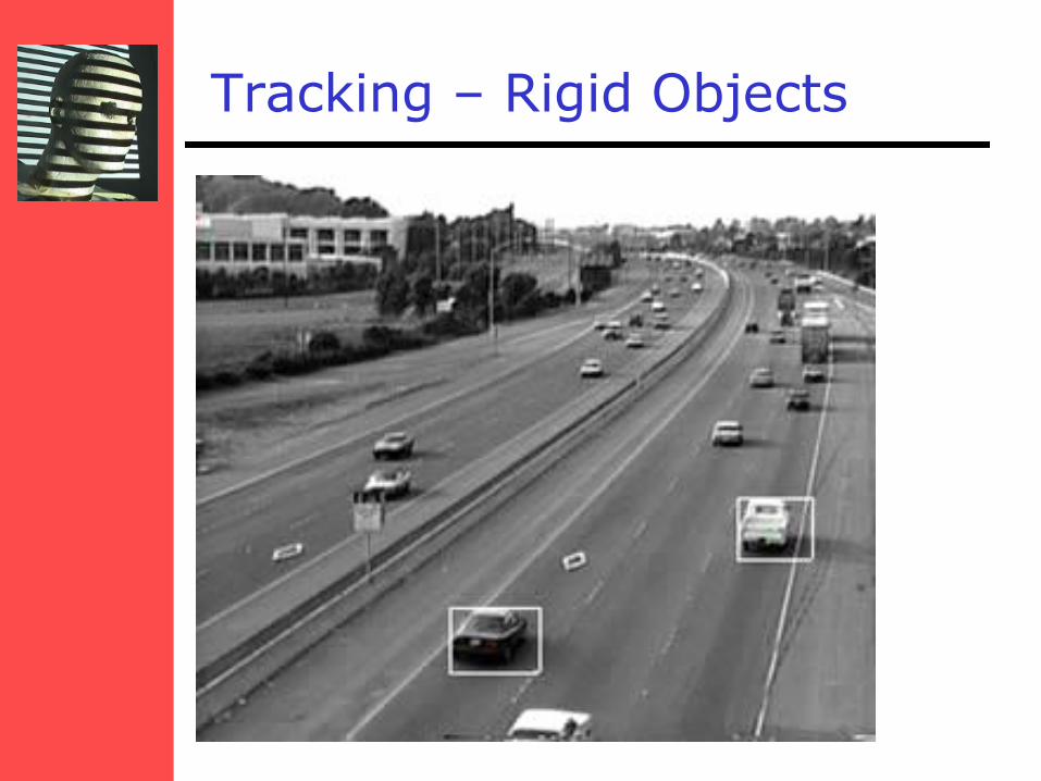
Tracking – Rigid Objects

)1( tI

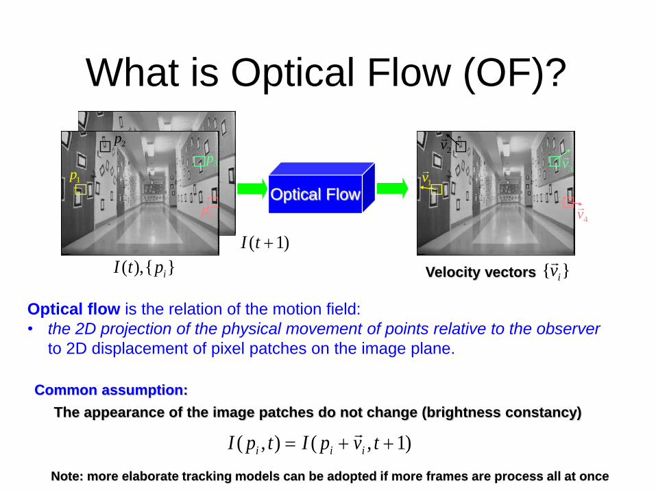
What is Optical Flow (OF)?

Optical Flow

}{),( iptI

1p

2p

3p

4p

1v

2v

3v

4v

}{ iv

Velocity vectors

Common assumption:

The appearance of the image patches do not change (brightness constancy)

)1,(),( tvpItpI iii

Note: more elaborate tracking models can be adopted if more frames are process all at once

Optical flow is the relation of the motion field:

• the 2D projection of the physical movement of points relative to the observer

to 2D displacement of pixel patches on the image plane.

Optical Flow

• Brightness Constancy

• The Aperture problem

• Regularization

• Lucas-Kanade

• Coarse-to-fine

• Parametric motion models

• Direct depth

• SSD tracking

• Robust flow

• Bayesian flow

Optical Flow and Motion

• We are interested in finding the movement of scene objects from time-varying images (videos).

• Lots of uses

– Motion detection

– Track objects

– Correct for camera jitter (stabilization)

– Align images (mosaics)

– 3D shape reconstruction

– Special effects

– Games: http://www.youtube.com/watch?v=JlLkkom6tWw

– User Interfaces: http://www.youtube.com/watch?v=Q3gT52sHDI4

– Video compression

7

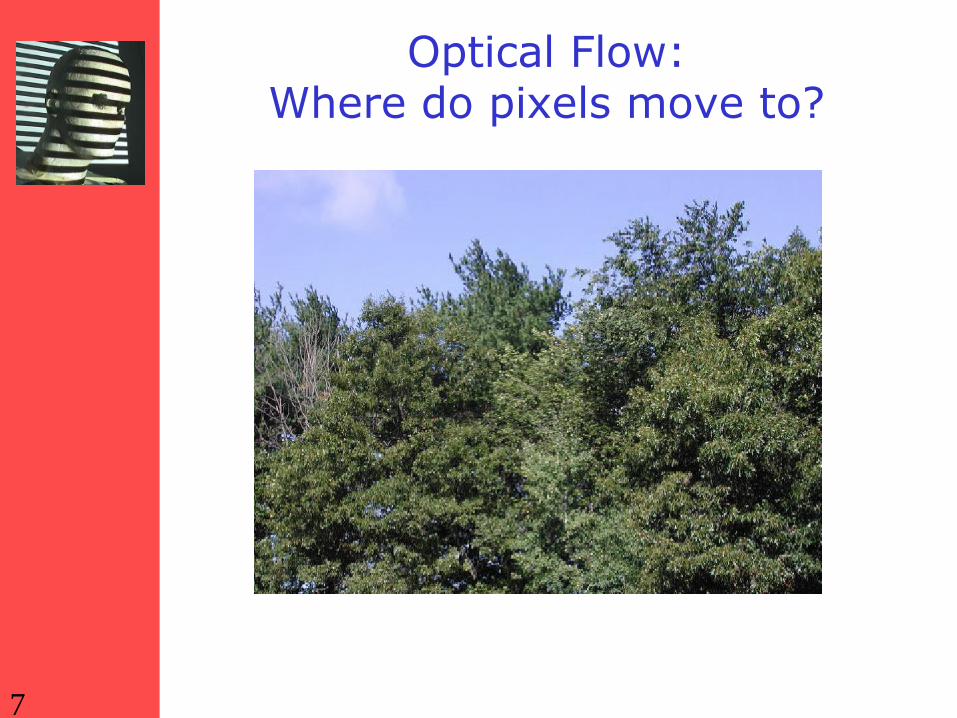
Optical Flow: Where do pixels move to?

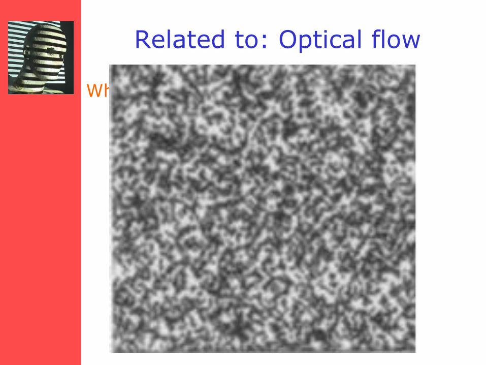
Related to: Optical flow

Where do pixels move?

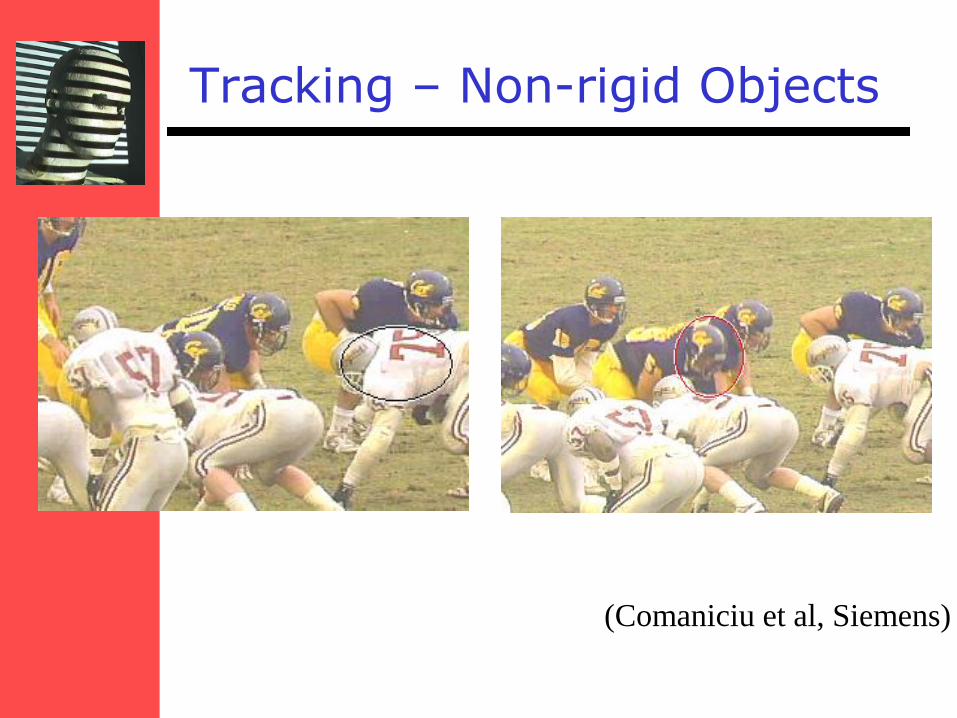
Tracking – Non-rigid Objects

(Comaniciu et al, Siemens)

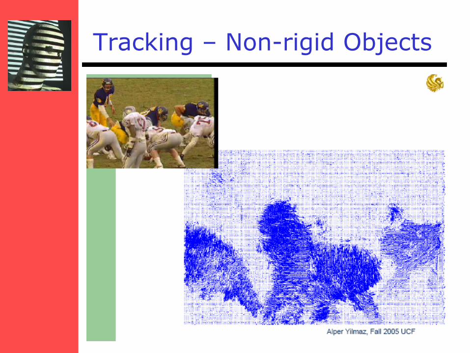
Tracking – Non-rigid Objects

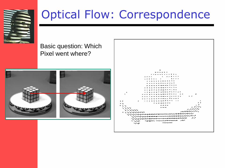
Optical Flow: Correspondence

Basic question: Which

Pixel went where?

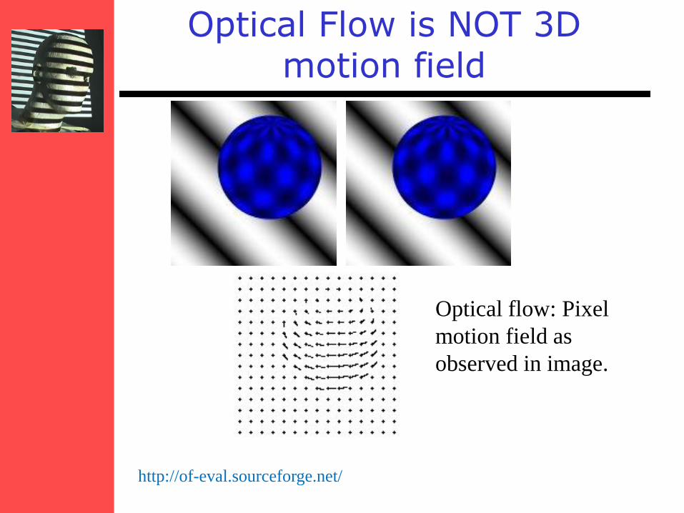
Optical Flow is NOT 3D motion field

http://of-eval.sourceforge.net/

Optical flow: Pixel

motion field as

observed in image.

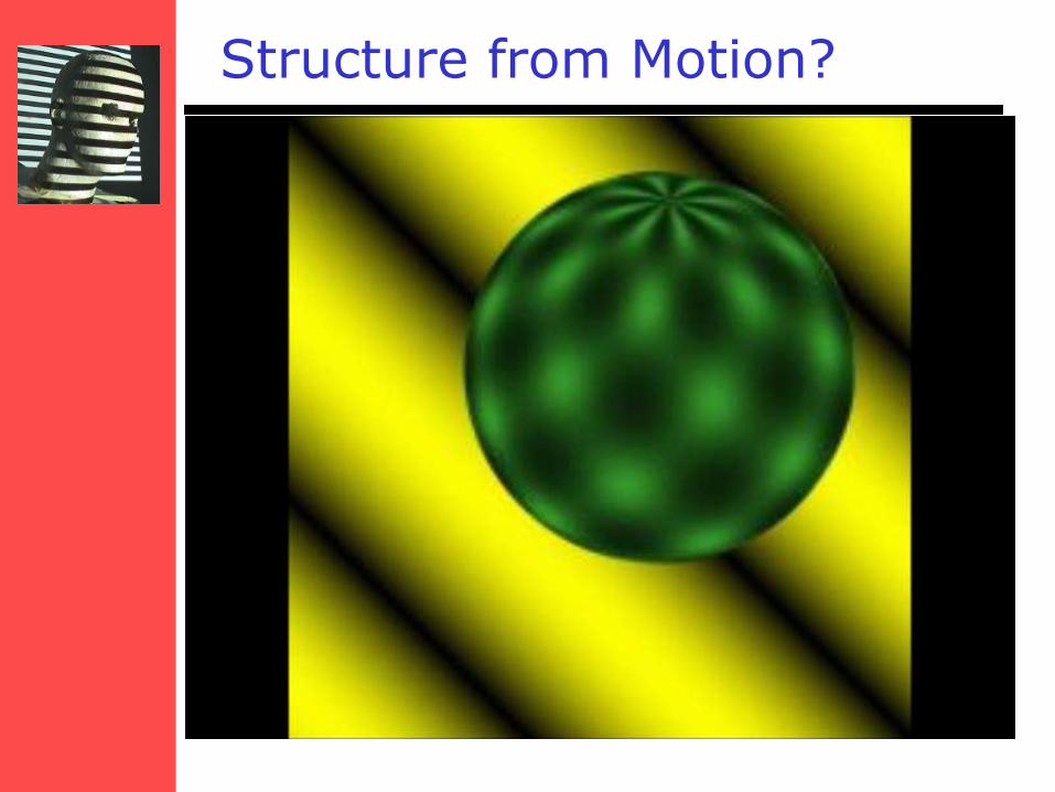
Structure from Motion?

• Known: optical flow

(instantaneous

velocity)

• Motion of camera /

object?

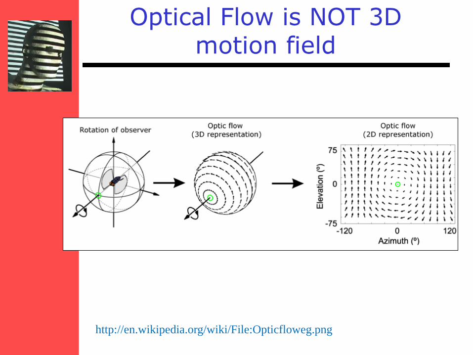
Optical Flow is NOT 3D motion field

http://en.wikipedia.org/wiki/File:Opticfloweg.png

15

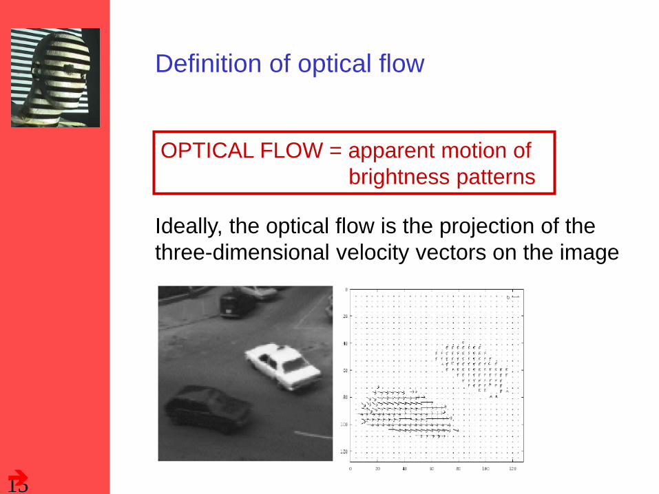
Definition of optical flow

OPTICAL FLOW = apparent motion of

brightness patterns

Ideally, the optical flow is the projection of the

three-dimensional velocity vectors on the image

16

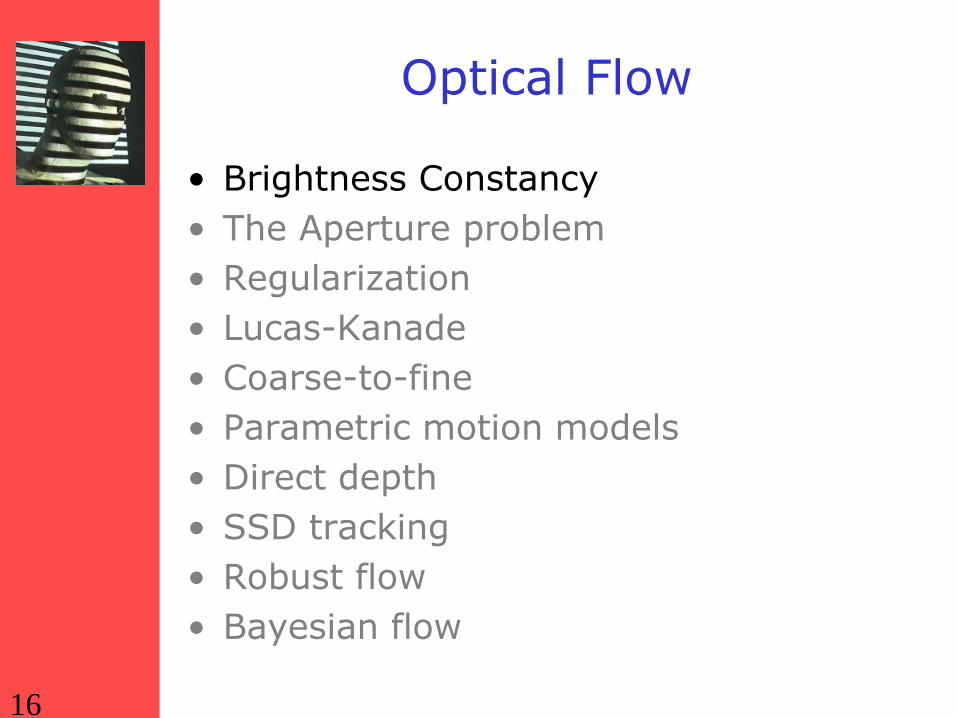
Optical Flow

• Brightness Constancy

• The Aperture problem

• Regularization

• Lucas-Kanade

• Coarse-to-fine

• Parametric motion models

• Direct depth

• SSD tracking

• Robust flow

• Bayesian flow

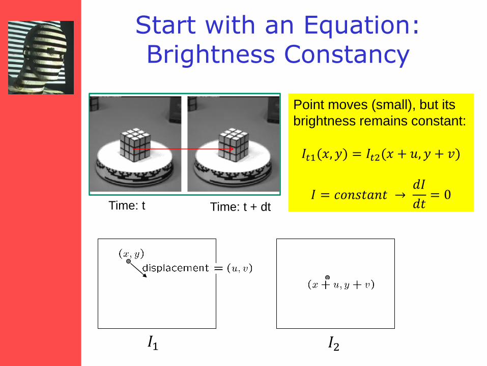
Start with an Equation: Brightness Constancy

Point moves (small), but its

brightness remains constant:

𝐼𝑡1(𝑥, 𝑦) = 𝐼𝑡2(𝑥 + 𝑢, 𝑦 + 𝑣)

𝐼 = 𝑐𝑜𝑛𝑠𝑡𝑎𝑛𝑡 → 𝑑𝐼

𝑑𝑡= 0

𝐼1 𝐼2

Time: t Time: t + dt

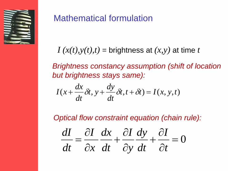
Mathematical formulation

I (x(t),y(t),t) = brightness at (x,y) at time t

Optical flow constraint equation (chain rule):

0

t

I

dt

dy

y

I

dt

dx

x

I

dt

dI

),,(),,( tyxItttdt

dyyt

dt

dxxI

Brightness constancy assumption (shift of location

but brightness stays same):

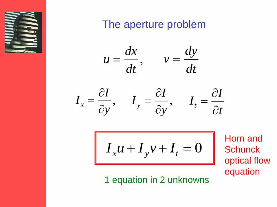
The aperture problem

0 tyx IvIuI

1 equation in 2 unknowns

dt

dxu

dt

dyv

y

II x

y

II y

t

II t

Horn and

Schunck

optical flow

equation

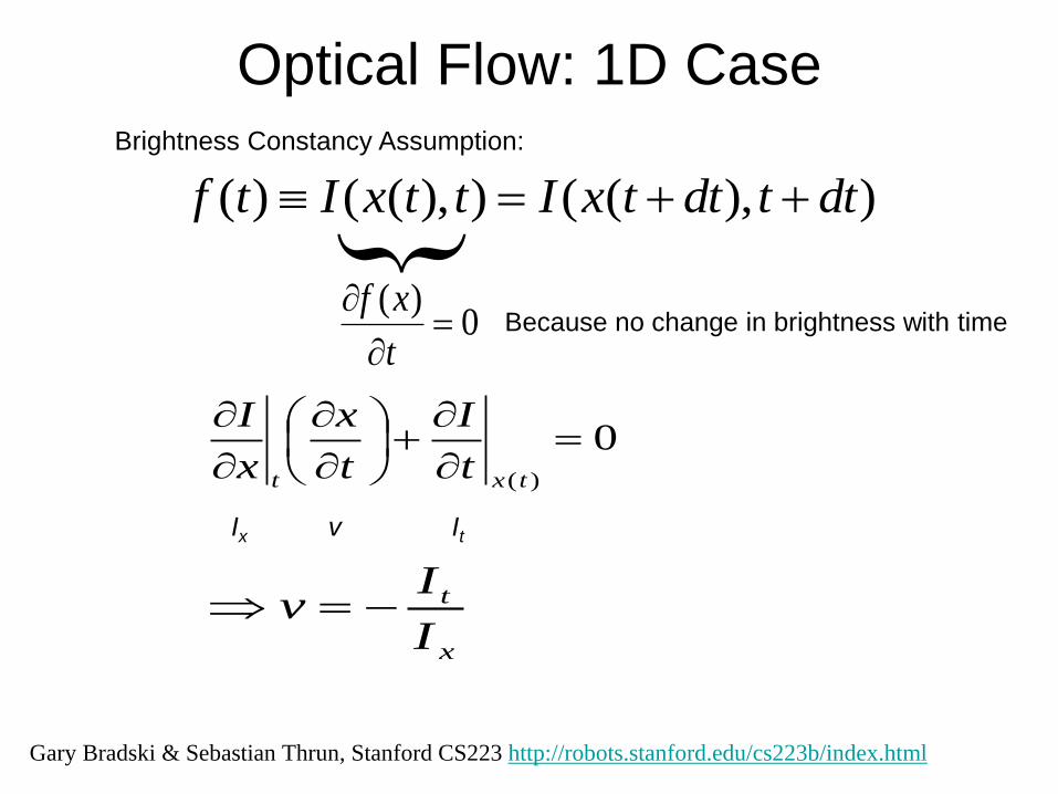
Optical Flow: 1D Case

Brightness Constancy Assumption:

)),(()),(()( dttdttxIttxItf

0)(

txt t

I

t

x

x

I

Ix v It

x

t

I

Iv

{

0)(

t

xfBecause no change in brightness with time

Gary Bradski & Sebastian Thrun, Stanford CS223 http://robots.stanford.edu/cs223b/index.html

21

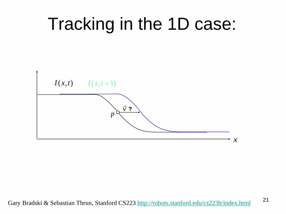
v

?

Tracking in the 1D case:

x

),( txI )1,( txI

p

Gary Bradski & Sebastian Thrun, Stanford CS223 http://robots.stanford.edu/cs223b/index.html

v

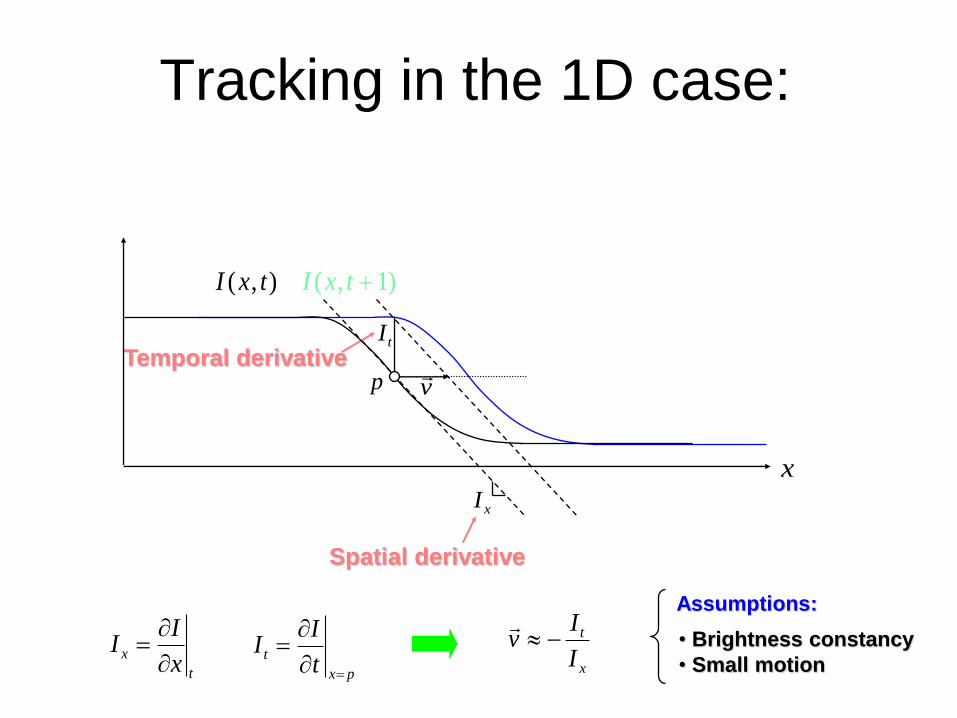
xI

Spatial derivative

Temporal derivative tI

Tracking in the 1D case:

x

),( txI )1,( txI

p

t

xx

II

px

tt

II

x

t

I

Iv

Assumptions:

• Brightness constancy

• Small motion

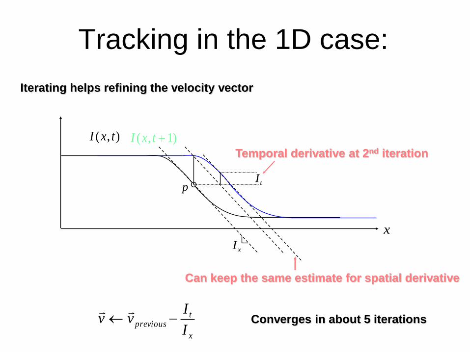
Tracking in the 1D case:

x

),( txI )1,( txI

p

xI

tI

Temporal derivative at 2nd iteration

Iterating helps refining the velocity vector

Can keep the same estimate for spatial derivative

x

tprevious

I

Ivv

Converges in about 5 iterations

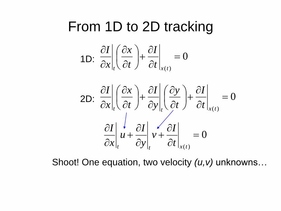
From 1D to 2D tracking

0)(

txt t

I

t

x

x

I1D:

0)(

txtt t

I

t

y

y

I

t

x

x

I2D:

0)(

txtt t

Iv

y

Iu

x

I

Shoot! One equation, two velocity (u,v) unknowns…

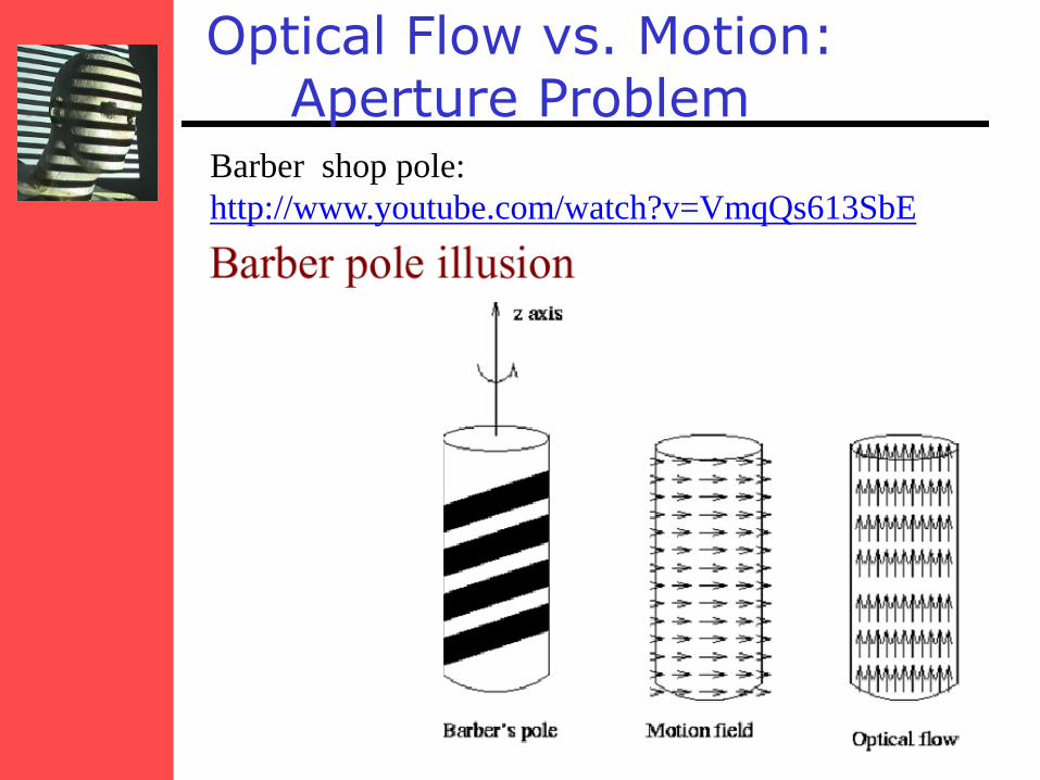
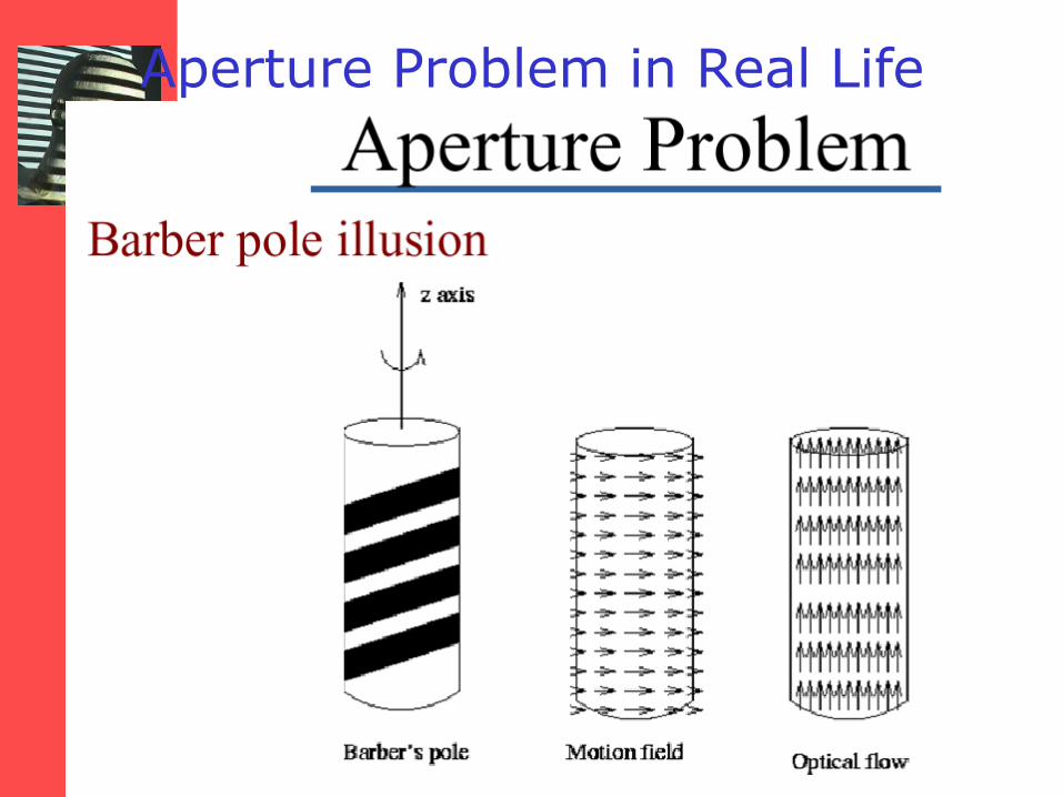
Optical Flow vs. Motion: Aperture Problem

Barber shop pole:

http://www.youtube.com/watch?v=VmqQs613SbE

26

Optical Flow

• Brightness Constancy

• The Aperture problem

• Regularization

• Lucas-Kanade

• Coarse-to-fine

• Parametric motion models

• Direct depth

• SSD tracking

• Robust flow

• Bayesian flow

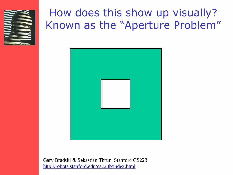
How does this show up visually? Known as the “Aperture Problem”

Gary Bradski & Sebastian Thrun, Stanford CS223

http://robots.stanford.edu/cs223b/index.html

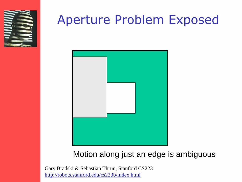
Aperture Problem Exposed

Motion along just an edge is ambiguous

Gary Bradski & Sebastian Thrun, Stanford CS223

http://robots.stanford.edu/cs223b/index.html

29

Aperture Problem in Real Life

30

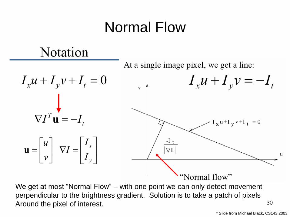
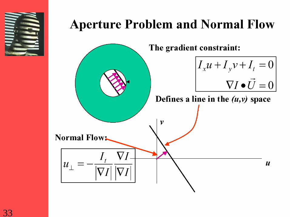
Normal Flow

* Slide from Michael Black, CS143 2003

We get at most “Normal Flow” – with one point we can only detect movement

perpendicular to the brightness gradient. Solution is to take a patch of pixels

Around the pixel of interest.

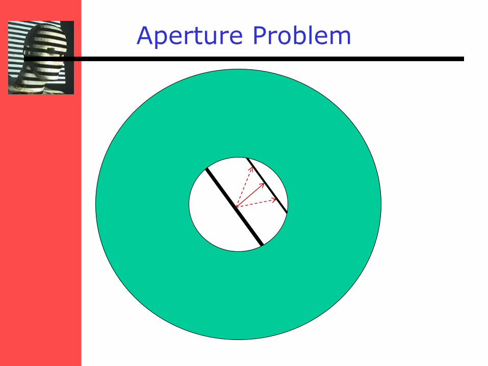
Aperture Problem

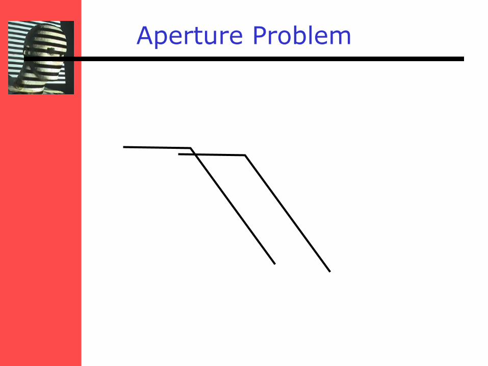
Aperture Problem

33

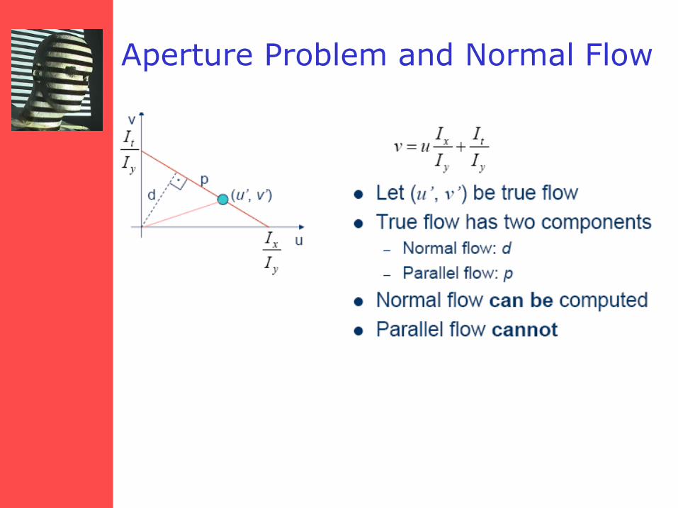
Aperture Problem and Normal Flow

Computing True Flow

• Horn & Schunck

• Schunck

• Lukas and Kanade

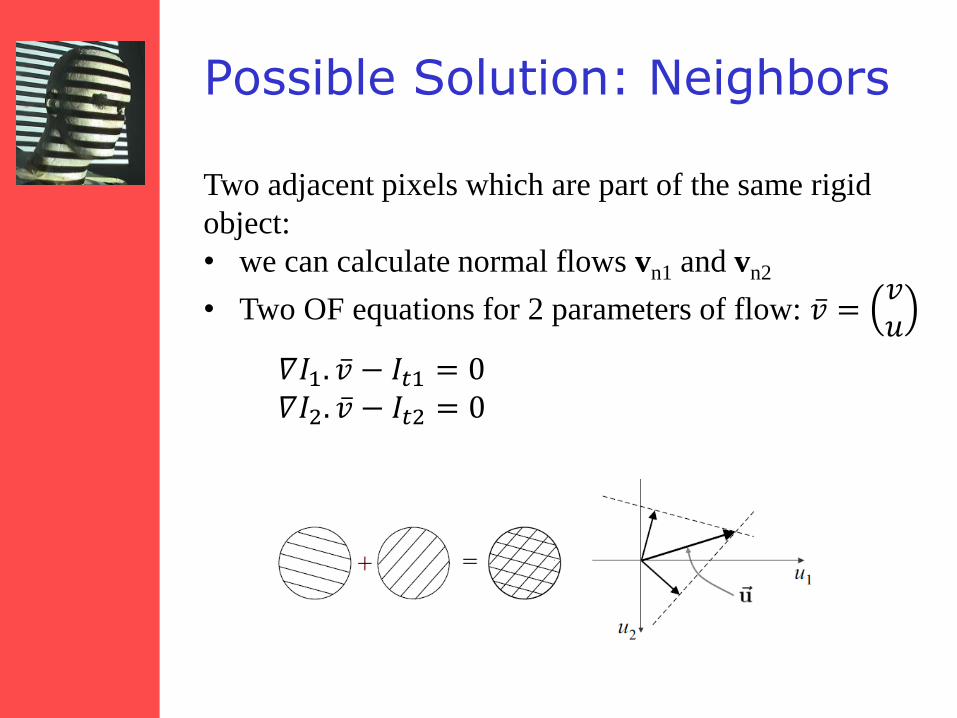
Possible Solution: Neighbors

Two adjacent pixels which are part of the same rigid

object:

• we can calculate normal flows vn1 and vn2

• Two OF equations for 2 parameters of flow: 𝑣 =𝑣𝑢

𝛻𝐼1. 𝑣 − 𝐼𝑡1 = 0

𝛻𝐼2. 𝑣 − 𝐼𝑡2 = 0

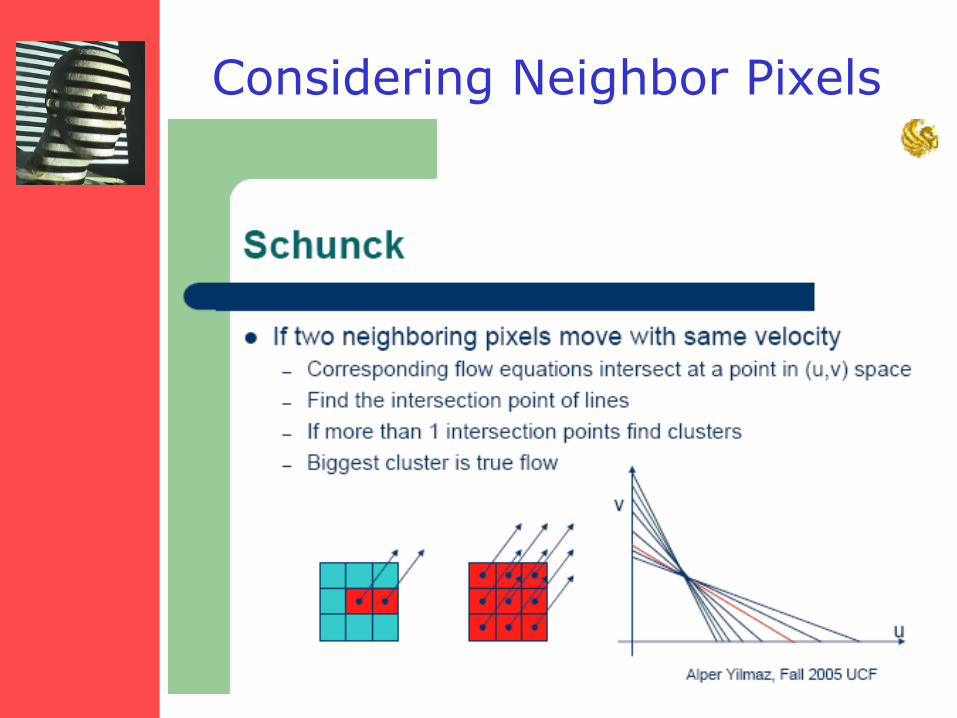
Considering Neighbor Pixels

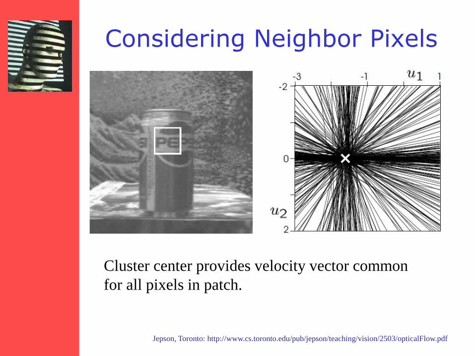
Considering Neighbor Pixels

Jepson, Toronto: http://www.cs.toronto.edu/pub/jepson/teaching/vision/2503/opticalFlow.pdf

Cluster center provides velocity vector common

for all pixels in patch.

39

Optical Flow

• Brightness Constancy

• The Aperture problem

• Regularization: Horn & Schunck

• Lucas-Kanade

• Coarse-to-fine

• Parametric motion models

• Direct depth

• SSD tracking

• Robust flow

• Bayesian flow

40

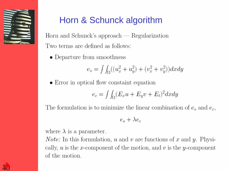
Horn & Schunck algorithm

41

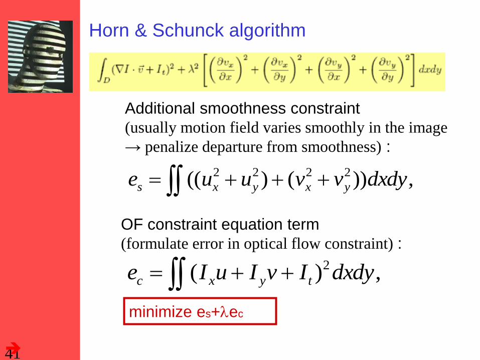
Horn & Schunck algorithm

Additional smoothness constraint

(usually motion field varies smoothly in the image

→ penalize departure from smoothness) :

,))()(( 2222 dxdyvvuue yxyxs

OF constraint equation term

(formulate error in optical flow constraint) :

,)( 2dxdyIvIuIe tyxc

minimize es+ec

42

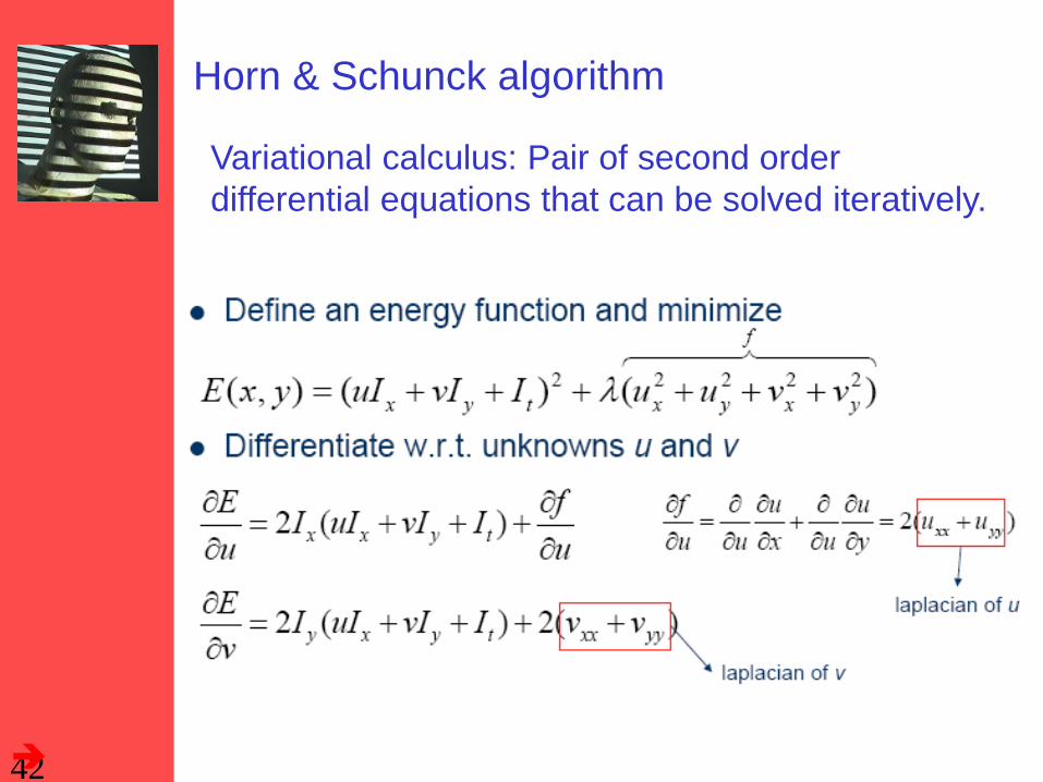
Horn & Schunck algorithm

Variational calculus: Pair of second order

differential equations that can be solved iteratively.

43

Horn & Schunck algorithm

44

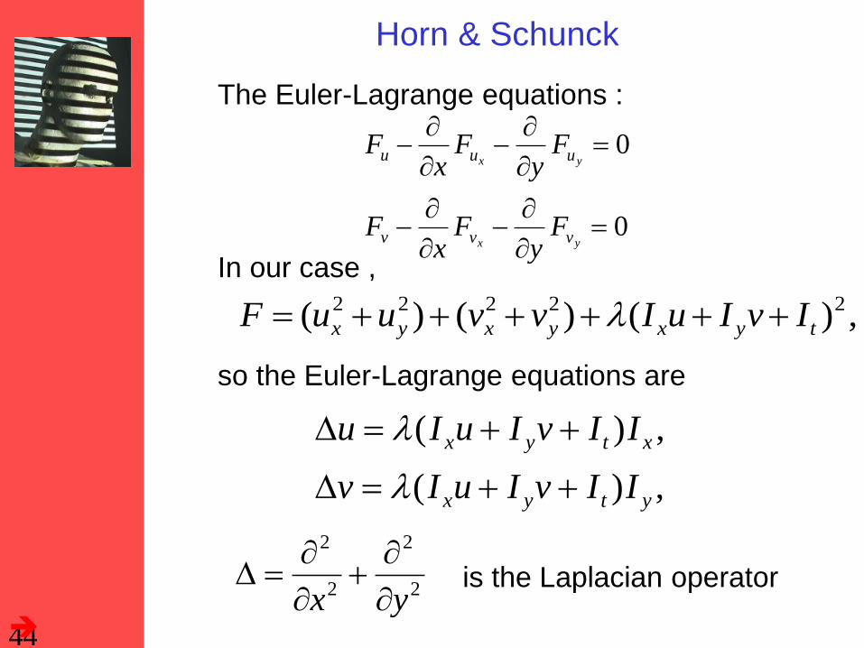
Horn & Schunck

The Euler-Lagrange equations :

0

0

yx

yx

vvv

uuu

Fy

Fx

F

Fy

Fx

F

In our case ,

,)()()( 22222

tyxyxyx IvIuIvvuuF

so the Euler-Lagrange equations are

,)(

,)(

ytyx

xtyx

IIvIuIv

IIvIuIu

2

2

2

2

yx

is the Laplacian operator

45

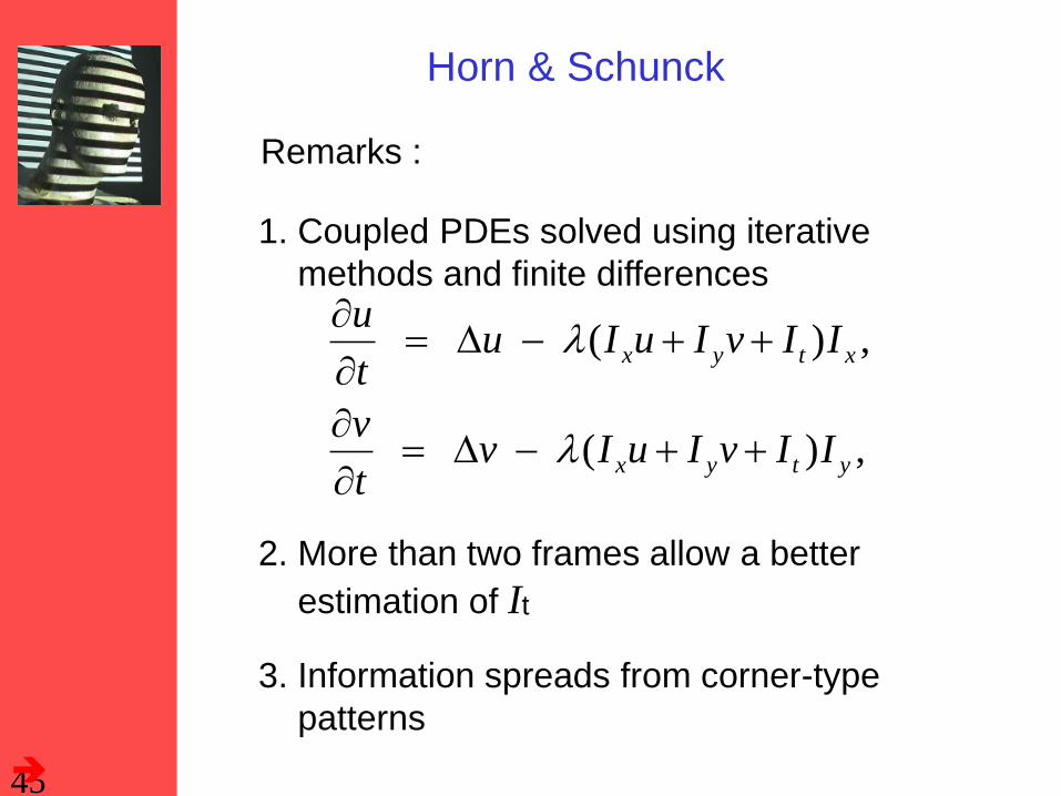
Horn & Schunck

Remarks :

1. Coupled PDEs solved using iterative

methods and finite differences

2. More than two frames allow a better

estimation of It

3. Information spreads from corner-type

patterns

,)(

,)(

ytyx

xtyx

IIvIuIvt

v

IIvIuIut

u

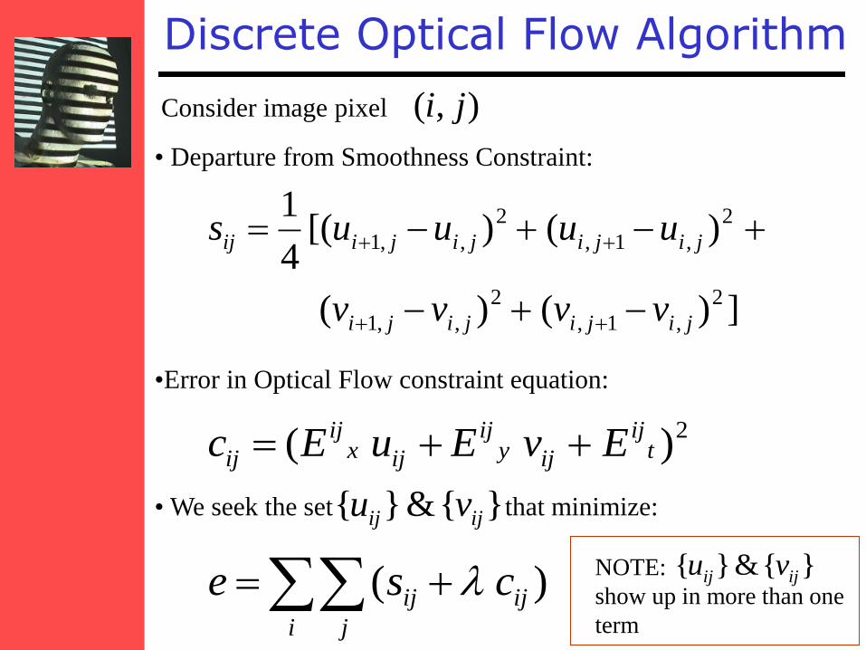
Discrete Optical Flow Algorithm

Consider image pixel

• Departure from Smoothness Constraint:

•Error in Optical Flow constraint equation:

• We seek the set that minimize:

i j

ijij cse )(

])()(

)()[(4

1

2

,1,

2

,,1

2

,1,

2

,,1

jijijiji

jijijijiij

vvvv

uuuus

2)( tij

ijyij

ijxij

ij EvEuEc

}{&}{ ijij vu

NOTE:

show up in more than one

term

}{&}{ ijij vu

),( ji

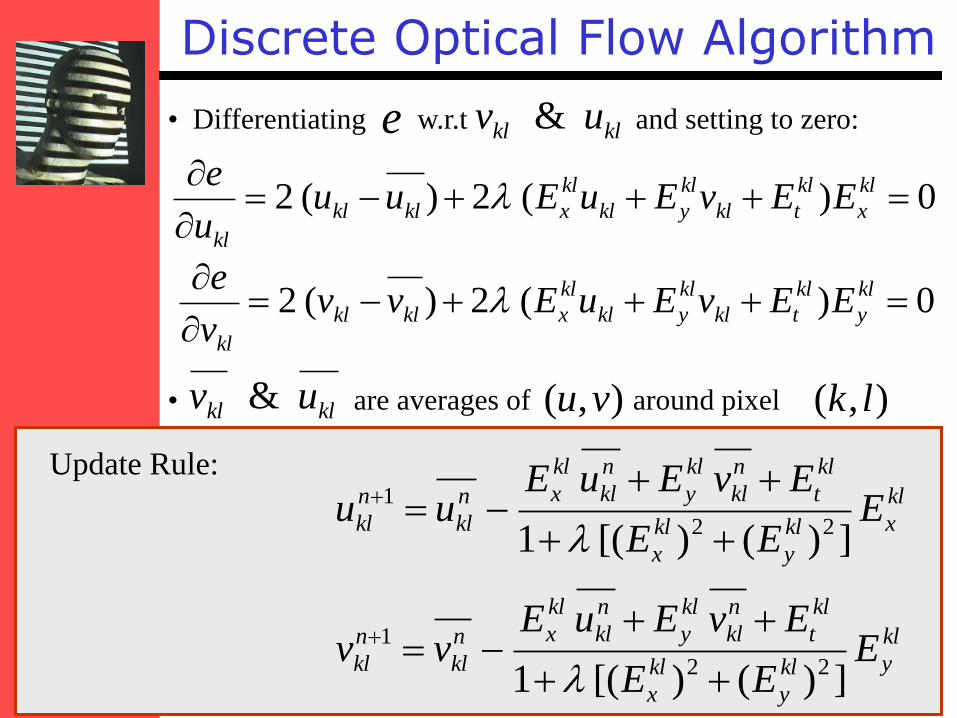
Discrete Optical Flow Algorithm

• Differentiating w.r.t and setting to zero:

• are averages of around pixel

e

0)(2)(2

kl

x

kl

tkl

kl

ykl

kl

xklkl

kl

EEvEuEuuu

e

0)(2)(2

kl

y

kl

tkl

kl

ykl

kl

xklkl

kl

EEvEuEvvv

e

klkl uv &

klkl uv & ),( lk),( vu

kl

xkl

y

kl

x

kl

t

n

kl

kl

y

n

kl

kl

xn

kl

n

kl EEE

EvEuEuu

])()[(1 22

1

kl

ykl

y

kl

x

kl

t

n

kl

kl

y

n

kl

kl

xn

kl

n

kl EEE

EvEuEvv

])()[(1 22

1

Update Rule:

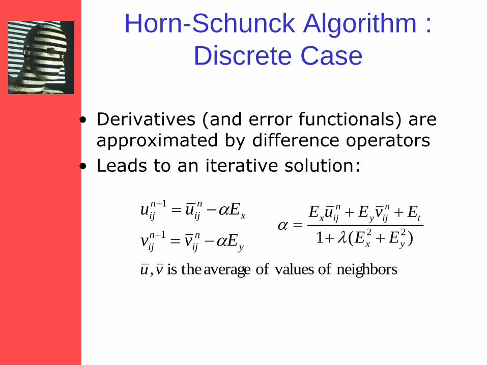
Horn-Schunck Algorithm :

Discrete Case

• Derivatives (and error functionals) are approximated by difference operators

• Leads to an iterative solution:

y

n

ij

n

ij

x

n

ij

n

ij

Evv

Euu

1

1

)(1 22

yx

t

n

ijy

n

ijx

EE

EvEuE

neighbors of valuesof average theis ,vu

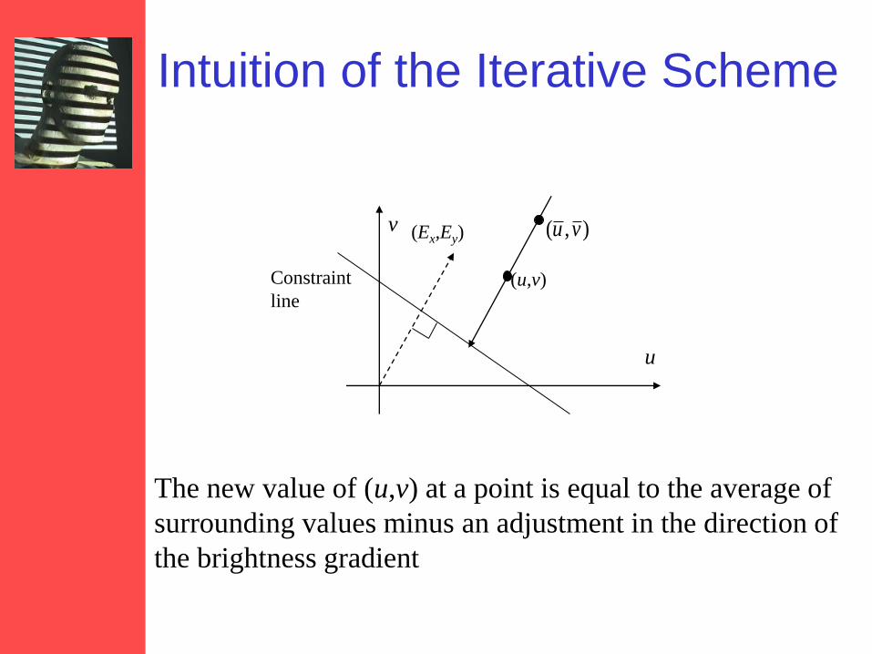
Intuition of the Iterative Scheme

u

v (Ex,Ey)

Constraint

line (u,v)

),( vu

The new value of (u,v) at a point is equal to the average of

surrounding values minus an adjustment in the direction of

the brightness gradient

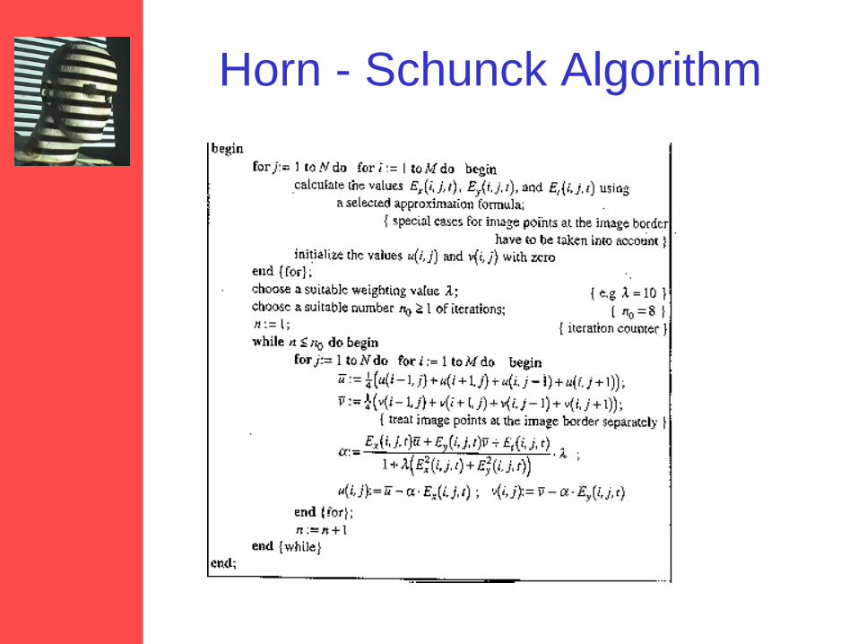
Horn - Schunck Algorithm

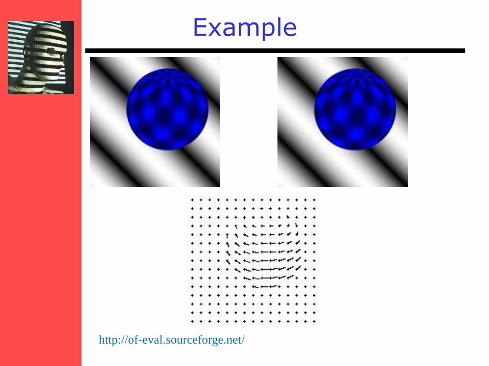
Example

http://of-eval.sourceforge.net/

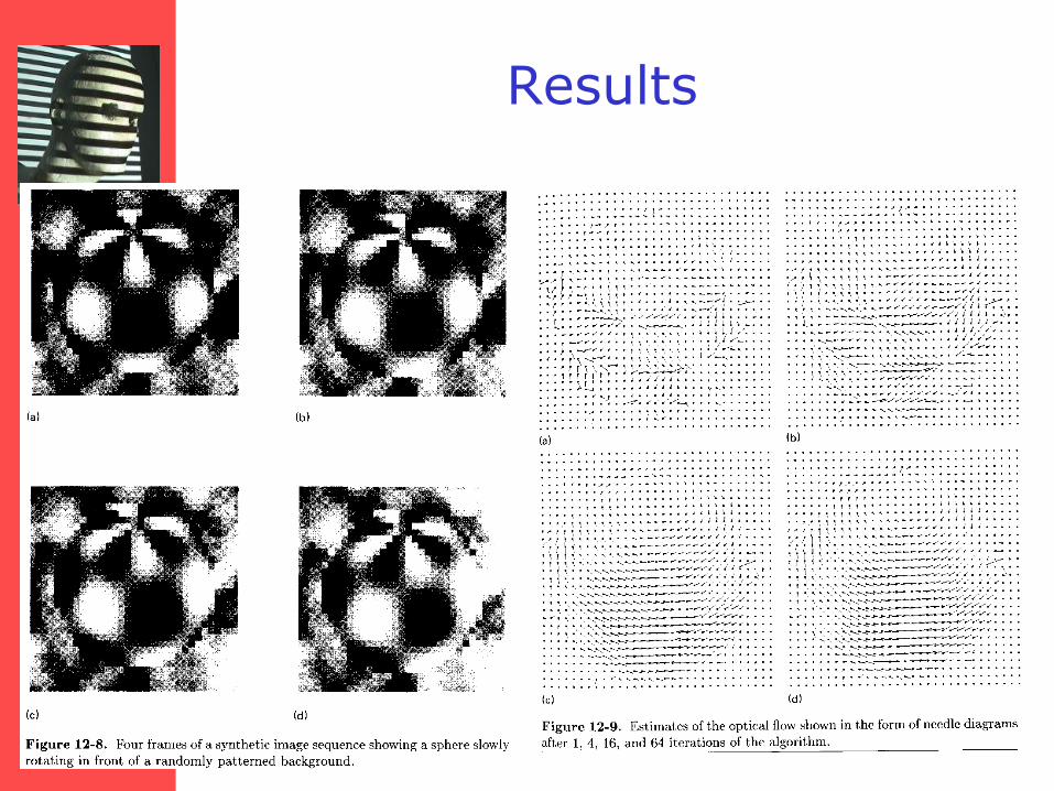
Results

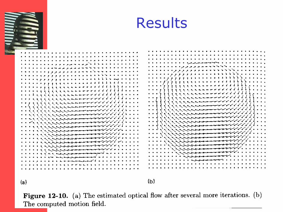
Results

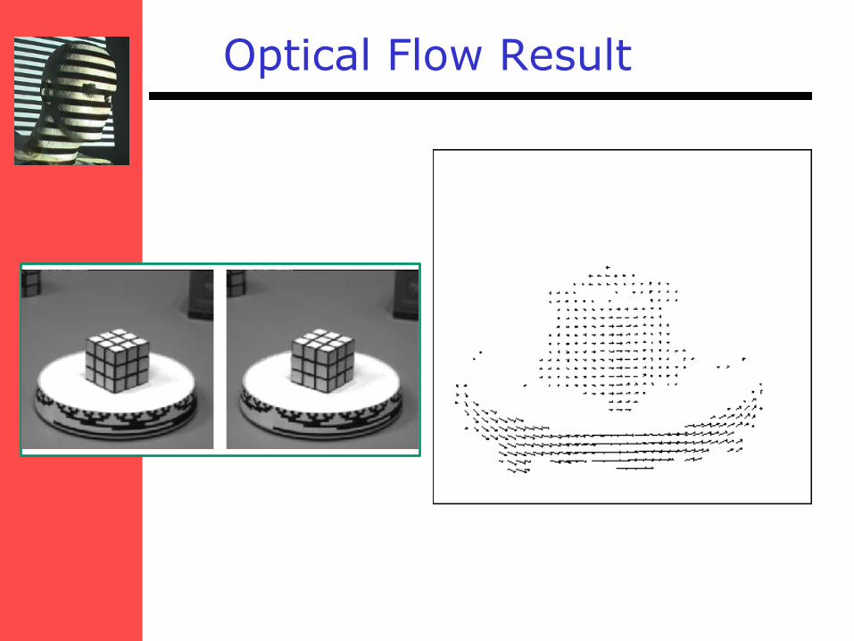
Optical Flow Result

56

Horn & Schunck, remarks

1. Errors at boundaries

2. Example of regularisation

(selection principle for the solution of

illposed problems)

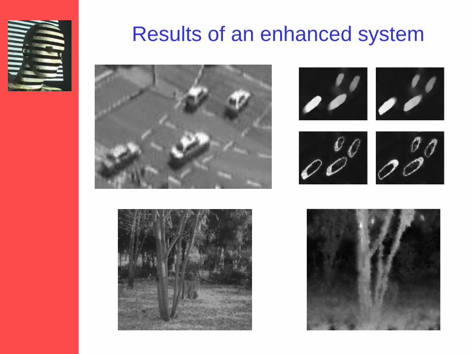
Results of an enhanced system

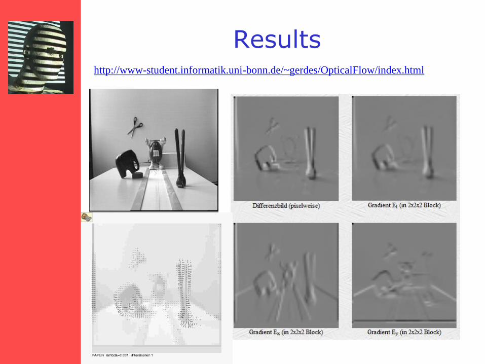
Results http://www-student.informatik.uni-bonn.de/~gerdes/OpticalFlow/index.html

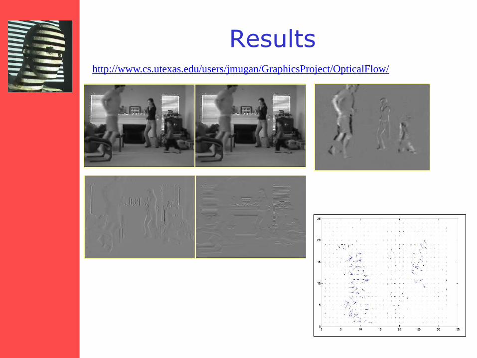
Results http://www.cs.utexas.edu/users/jmugan/GraphicsProject/OpticalFlow/

60

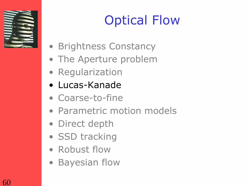
Optical Flow

• Brightness Constancy

• The Aperture problem

• Regularization

• Lucas-Kanade

• Coarse-to-fine

• Parametric motion models

• Direct depth

• SSD tracking

• Robust flow

• Bayesian flow