HAL Id: hal-01930498https://hal.inria.fr/hal-01930498

Submitted on 22 Nov 2018

HAL is a multi-disciplinary open accessarchive for the deposit and dissemination of sci-entific research documents, whether they are pub-lished or not. The documents may come fromteaching and research institutions in France orabroad, or from public or private research centers.

L’archive ouverte pluridisciplinaire HAL, estdestinée au dépôt et à la diffusion de documentsscientifiques de niveau recherche, publiés ou non,émanant des établissements d’enseignement et derecherche français ou étrangers, des laboratoirespublics ou privés.

Optical Flow For Image-Based River Velocity EstimationMusaab Khalid, Lionel Pénard, Etienne Mémin

To cite this version:Musaab Khalid, Lionel Pénard, Etienne Mémin. Optical Flow For Image-Based River Ve-locity Estimation. Flow Measurement and Instrumentation, Elsevier, 2019, 65, pp.110-121.10.1016/j.flowmeasinst.2018.11.009. hal-01930498

Author’s Accepted Manuscript

Optical Flow For Image-Based River VelocityEstimation

M. Khalid, L. Pénard, E. Mémin

PII: S0955-5986(18)30026-8DOI: https://doi.org/10.1016/j.flowmeasinst.2018.11.009Reference: JFMI1501

To appear in: Flow Measurement and Instrumentation

Received date: 22 January 2018Revised date: 8 September 2018Accepted date: 10 November 2018

Cite this article as: M. Khalid, L. Pénard and E. Mémin, Optical Flow ForImage-Based River Velocity Estimation, Flow Measurement andInstrumentation, https://doi.org/10.1016/j.flowmeasinst.2018.11.009

This is a PDF file of an unedited manuscript that has been accepted forpublication. As a service to our customers we are providing this early version ofthe manuscript. The manuscript will undergo copyediting, typesetting, andreview of the resulting galley proof before it is published in its final citable form.Please note that during the production process errors may be discovered whichcould affect the content, and all legal disclaimers that apply to the journal pertain.

www.elsevier.com/locate/flowmeasinst

Optical Flow For Image-Based River Velocity Estimation

M. Khalida, L. Pénarda, E. Méminb

aIrstea, UR RiverLy, centre de Lyon-Villeurbanne, 5 rue de la Doua CS 20244, 69625Villeurbanne, France

bFluminance, Inria/Irstea/IRMAR, Campus de Beaulieu, 35042 Rennes, France

Abstract

We present a novel motion estimation technique for image-based river velocimetry. Itis based on the so-called optical flow, which is a well developed method for rigid mo-tion estimation in image sequences, devised in computer vision community. Contraryto PIV (Particle Image Velocimetry) techniques, optical flow formulation is flexibleenough to incorporate physics equations that govern the observed quantity motion.Over the past years, it has been adopted by experimental fluid dynamics communitywhere many new models were introduced to better represent different fluids motions,(see (Heitz et al., 2010) for a review). Our optical flow is based on the scalar transportequation and is augmented with a weighted diffusion term to compensate for smallscale (non-captured) contributions. Additionally, since there is no ground truth datafor such type of image sequences, we present a new evaluation method to assess theresults. It is based on trajectory reconstruction of few Lagrangian particles of interestand a direct comparison against their manually-reconstructed trajectories. The newmotion estimation technique outperformed traditional optical flow and PIV-basedmethods.Keywords: Optical Flow, River Velocimetry, PIV, LSPIV

1. Introduction

To estimate the velocity of the free surface of a river using image-based techniques,there are two main issues to be addressed. The first is the 2D motion estimation inimage space and the second issue is about how to transform 2D image estimationsback to 3D. It should also handle the scaling of these estimations to their true physicalscale. The metric surface velocity could be then obtained using the time betweenimages. It is a valuable piece of information to compute rivers discharge using thewell-known velocity-area method. The work presented here focuses on the first issue.We specifically target rivers with noticeable discharge or urban inundations. Inthese settings, the free surface manifests a visible and probably turbulent translatorymotion.

For many years, PIV (Particle Image Velocimetry) (Adrian, 1991) was the onlytechnique available for fluid motion estimation in image sequences. PIV computes the

Preprint submitted to Flow Measurement and Instrumentation November 15, 2018

displacement between windows of a certain size in two consecutive images depictingspatio-temporal evolution of a fluid. These windows are tracked assuming a trans-lational motion between images using some measure of similarity that is computedon them. To compute better similarity scores, the flow has to be well-seeded withparticles. As a consequence, PIV faces strong difficulties on scalar images in whichmany areas have low intensity gradient. In many cases, there is a necessary post-processing step to correct or remove spurious vectors, inevitably generated in regionswith low intensity gradient. The post-processing step is also used to interpolate thesparse vector field to generate a denser one. In addition, choosing a suitable windowsize is a tricky task, one needs bigger window to accumulate more information forbetter score computation, but then the bigger the window, the more likely it containscomplex motions far from the window’s translational motion assumption. Despite itswide-spread usage specially in controlled lab environments, PIV lacks sound physicsfoundation, it treats all image sequences equally, regardless of the nature of the objectin motion. Furthermore, it only computes sparse estimations, many of them mightbe discarded in the post-processing phase. In their seminal paper, Fujita et al. (1998)took PIV outside the lab to measure the velocity of rivers in ortho-rectified imagesequences. The ortho-rectification applies geometric transformation to produce newset of images in which the perspective effect is removed. The ortho-rectified sequenceis produced in such a way that their real spatial resolution is now known. The imagemotion estimation technique (PIV in this case) is then applied to the newly createdsequence. Hence, the name of their method LSPIV (Large Scale Particle Image Ve-locimetry) which became the benchmark for image-based river velocimetry (Jodeauet al., 2008, Dramais et al., 2011, Muste et al., 2014).

If we closely examine the original problem as depicted in Figure (1.1), the motionin 3D space is captured by a camera and as a result, a 2D motion is observed inimages. The image-based velocimetry problem is exactly solved by taking the reverseroute. We can distinguish the two aforementioned issues or steps that need to besolved along this route. Most LSPIV works however mix the two steps together whichmakes it difficult to determine the exact sources of uncertainty and the effects of eachstep error to the overall error. It is a valid idea to take the route shown by the bluearrows in Figure (1.1) and treat each issue individually. Recently, Patalano et al.(2017) applied the ortho-rectification only to the results but the motion estimationwas separately applied to the original obliquely-viewed images. This paper focusesonly on the first step, that is, motion estimation of river surface in image space.

Due to PIV limitations cited above, we found the so-called Optical Flow (Horn andSchunck, 1981) to be well adapted to fluids. A nice review paper on the applicationof optical flow to fluids could be find in (Heitz et al., 2010).

2

Figure 1.1: 3D motion projection to images.

Previous work

Stemmed from computer vision community in the early 80s due to Horn andSchunck (1981) work. Optical flow consists of an energy functional to be minimized.It combines the information that could be extracted from images (called data term)and the expected solutions set (called regularization term) in a concise and unam-biguous way: ∫

Ω

(∂I

∂t+∇I·ω

)2

+ α ‖∇ω‖2

dX (1.1)

where ∇ represents the spatial gradient for both image intensity function I and the 2Dvelocity field ω = [u, v]. A parameter α is introduced to define the trade-off betweenthe data term and the regularization term. The first quadratic term (data term) iscalled the brightness constancy (BC). It assumes that points conserve their brightnessvalue captured by the camera while moving in a small time interval. The second termis trying to minimize velocity gradient globally, assuming that neighbouring pointsbelong normally to the same surface and tend to move together. This assumptionresembles the one made in PIV that all points in the window have the same velocity.However, its formulation in optical flow is more relaxed, velocities of points on thesame neighbourhood could vary, but this variation should be limited. This modelwitnessed many improvements over the years to overcome its limitations.

First of all, the BC assumption used in the data term in (1.1) is derived us-ing Taylor approximation to linearize the original non-linear pattern matching BC,I(X(t), t) = I(X(t + 1), t + 1). The linearized model assumes very small motionwhich is indeed not the case in general. To deal with large displacements, the use ofdifferent image resolutions in a hierarchical, coarse-to-fine way (called image pyra-mid) has been introduced (Bergen et al., 1992). This strategy is improved by using

3

warping steps in which the second image is brought closer to the first image usingthe estimated velocity field of the previous pyramid level (Mémin and Pérez, 1998,2002). Consequently, only a small increment is sought at each level.

Secondly, the quadratic penalization is known to be sensitive to outliers. Thisis particularly seen in image regions with discontinuities where we might have twodifferent objects moving in different directions at different speeds. The quadraticpenalization tends to average these two motions which results in a solution clearly notin agreement with the real motion at the discontinuity area and around it. Black andAnandan (1996) proposed to use robust penalization methods to cope with outliers.This procedure gave better results i.e. sharper discontinuities.

Lastly, the BC assumption might not hold in many cases due to occlusions, imag-ing acquisition quality and/or illumination changes caused by surface reflections forinstance. Therefore, it is a good practice to use a robust function for the dataterm as well (Mémin and Pérez, 1998). Other notable improvements were proposedby Mémin and Pérez (1998), Brox et al. (2004) in which authors used the origi-nal non-linear version of BC. The resulting non-linear equation is solved iterativelyusing a multi-grid optimization technique (Mémin and Pérez, 1998) or a Graduated-Non-Convexity (GNC) (Blake and Zisserman, 1987) with two fixed point iterationsoptimization technique. Median filtering of intermediate flow (between pyramid lev-els) showed very good performance regarding outliers rejection. Sun et al. (2014)elaborated on this and showed that it is a different energy function when medianfiltering is utilized.

The functional (1.1) was designed for rigid or quasi-rigid motions as they are themost encountered in natural scenes. Fluids in general have more complex motionpatterns. Liu and Shen (2008) formally established the relationship between opticalflow and fluid flow based on the perspective projection of the transport equation onthe 2D plane and found that optical flow is proportional to the path-averaged veloc-ity field weighted with a relevant field quantity. This gave the physical foundationneeded since the BC assumption is not based on any physical principle. Higher orderregularization has been proposed before by Suter (1994) based on the divergence andthe curl of the vector field. However, minimizing such high order terms is known to beproblematic. Corpetti et al. (2005) proposed a relaxed and easier term to minimizethe gradient of divergence and curl. They also suggested a data term based on theIntegrated Continuity Equation. They also showed that, from an optimization pointof view, the L2 regularization in equation (1.1) is equivalent to penalizing divergenceand curl equally, which might be a problem depending on the fluid at hand. Heitzet al. (2008) suggested to refrain from multi-resolution strategy for PIV applicationsbecause the smoothing and sub-sampling of images will suppress the particles in thecoarsest resolution levels. They introduced a model that combines local information(PIV) with a global dense optical flow formulation. A very promising line of researchconsists of deriving new data term based on LES (Large Eddy Simulation) of thetransport equation (Cassisa et al., 2011, Chen et al., 2015). The latter used a di-vergence norm penalization term as regularization to conserve the curl of the vectorfield. This derivation from transport equation separates the effects of information

4

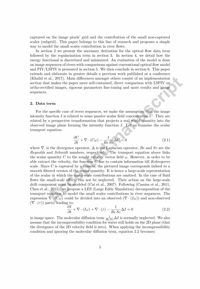
captured on the image pixels’ grid and the contribution of the small non-capturedscales (subgrid). This paper belongs to this line of research and proposes a simpleway to model the small scales contribution in river flows.

In section 2 we present the necessary derivation for the optical flow data termfollowed by the regularization term in section 3. In section 4, we detail how theenergy functional is discretized and minimized. An evaluation of the model is doneon image sequences of rivers with comparisons against conventional optical flow modeland PIV/LSPIV is presented in section 5. We then conclude in section 6. This paperextends and elaborate in greater details a previous work published at a conference(Khalid et al., 2017). Main differences amongst others consist of an implementationsection that makes the paper more self-contained, direct comparison with LSPIV onortho-rectified images, rigorous parameters fine-tuning and more results and imagesequences.

2. Data term

For the specific case of rivers sequences, we make the assumption that the imageintensity function I is related to some passive scalar field concentration C. They arerelated by a perspective transformation that projects a real world quantity into theobserved image plane forming the intensity function I. Let us examine the scalartransport equation:

∂C

∂t+∇ · (Cω)− 1

ReSc∆C = 0 (2.1)

where ∇· is the divergence operator, ∆ is the Laplacian operator, Re and Sc are theReynolds and Schmidt numbers, respectively. The transport equation above linksthe scalar quantity C to the sought velocity vector field ω. However, in order to beable extract the velocity, the function C has to contain information till Kolmogorovscale. Since C is captured by a camera, the pictured image corresponds indeed to asmooth filtered version of the scalar quantity. It is hence a large-scale representationof the scalar in which the small-scale contributions are omitted. In the case of fluidflows the small-scale effects can not be neglected. Their action on the large-scaledrift component must be modeled (Cui et al., 2007). Following (Cassisa et al., 2011,Chen et al., 2015), we propose a LES (Large Eddy Simulation) decomposition of thetransport equation to model the small scales contributions in river sequences. Theexpression ∇ · (Cω) could be divided into an observed (∇ · (Iω)) and non-observed(∇ · (τ)) parts, leading to:

∂I

∂t+∇ · (Iω) +∇ · (τ)− 1

ReSc∆I = 0 (2.2)

in image space. The molecular diffusion term 1ReSc∆I is normally neglected. We also

assume that the incompressibility condition for water still holds on the 2D plane (thatthe divergence of the 2D velocity field is zero). When applying the incompressibilitycondition and ignoring the molecular diffusion term, equation 2.2 becomes:

5

∂I

∂t+∇I · ω +∇ · (τ) = 0 (2.3)

We see that the BC assumption appears again in addition to the new subgrid term,which means conventional optical flow is consistent with this physics-based deriva-tion. As suggested by Cassisa et al. (2011), the non-observed term is consideredrelated to turbulent viscosity τ = −Dt∇I where Dt is a turbulent diffusion coeffi-cient. We opted for a simple model to estimate Dt using previous velocity estimationswithin the sequence and/or the pyramid levels of image pair at hand. We feed thesevelocity estimations to Prandtl mixing-length model (Prandtl, 1925). This modeluses the streamwise velocity u and the Mixing Length l to estimate the turbulentviscosity νt = l2

∣∣∣dudy ∣∣∣. This quantity is relevant for the computation of Dt =νt

sctwhere

sct is the turbulent Schmidt number which has an empirical value usually determinedexperimentally. It has been reported that sct has widespread values between 0.2 and3 in general (Tominaga and Stathopoulos, 2007) while other authors very recentlysuggested values around 1 to be optimal on a tracer transport study (Gualtieri et al.,2017). Accordingly, Dt is considered equal to νt. The Mixing Length l is defined asthe distance traversed by a fluid parcel before it becomes blended in with neighbour-ing masses. To the best of our knowledge, there is no clear way to predict this valuefrom images. It is taken here to be 1 because the differential optical flow formulationassumes infinitesimal displacements that don’t exceed one pixel.

Due to sources or sinks in the fluid, the imaged surface is prone to intermittentchanges because of out of plane (depth) motions. Some regions may rise up or sinkdown during the temporal evolution of the fluid causing changes in the intensityfunction. As a result, the brightness consistency assumption might not hold in manylocations. Thus, a robust function is chosen for the data term. In practice we mainlyuse the Lorentzian function (Black and Anandan, 1996) but there are many othersthat could be used. The data term reads:∫

Ω

Ψ

(∥∥∥∥∂I∂t +∇I · ω +∇ · (−Dt∇I)

∥∥∥∥2)

where Ψ is the robust function. This could be further simplified as:∫Ω

Ψ

(∥∥∥∥∂I∂t +∇I · ω −Dt∆I

∥∥∥∥2)

(2.4)

which is the proposed data term.

3. Regularization

Regarding the regularization, two main choices were made. Firstly, it can benoticed that usually the river flows of interest do not exhibit strong large-scale ed-dies motion. Rivers with such eddies have indeed less interest in river velocimetry

6

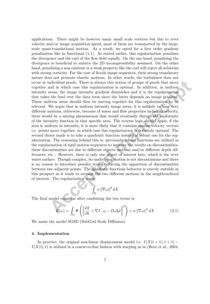
applications. There might be however many small scale vortices but due to rivervelocity and/or image acquisition speed, most of them are transported by the large-scale quasi-translational motion. As a result, we opted for a first order gradientpenalization like in functional (1.1). As stated earlier, this regularization penalizesthe divergence and the curl of the flow field equally. On the one hand, penalizing thedivergence is beneficial to enforce the 2D incompressibility assumed. On the otherhand, penalizing a non existent or a weak property like the curl will reject all solutionswith strong vorticity. For the case of floods image sequences, their strong translatorynature does not promote chaotic motions. In other words, the turbulence does notoccur at individual pixels. There is always this notion of groups of pixels that movetogether and in which case this regularization is optimal. In addition, in uniformintensity areas, the image intensity gradient diminishes and it is the regularizationthat takes the lead over the data term since the latter depends on image gradient.These uniform areas should then be moving together for this regularization to berelevant. We argue that in uniform intensity image areas, it is unlikely to have verydifferent motions, otherwise, because of water and flow properties including velocity,there would be a mixing phenomenon that would eventually disrupt the uniformityof the intensity function in that specific area. The reverse logic should apply, if thearea is uniform in intensity, it is more likely that it contains similar velocity vectorsi.e. points move together, in which case this regularization is definitely optimal. Thesecond choice made is to take a quadratic function instead of robust one for the reg-ularization. The reasoning behind this is: previously robust functions are utilized inthe regularization of rigid motion sequences to improve the results on discontinuities,these discontinuities are due to different objects motions and/or different depth dif-ferences, etc... However, there is only one object of interest here, which is the riverwater surface. Though complex, its underlying motion is not discontinuous and thereis no reason to introduce penalty terms enforcing the apparition of discontinuitiesbetween two adjacent points. The quadratic functions behavior is exactly suitable inthis prospect as it tends to average the two different motions in the neighbourhoodof interest. The regularization reads:∫

Ω

α ‖∇ω‖2 dX

The final model equation after combining the two terms is:

E(ω) =

∫Ω

Ψ

(∥∥∥∥∂I∂t +∇I · ω −Dt∆I

∥∥∥∥2)

+ α ‖∇ω‖2 dX (3.1)

We name the model SGSD (SubGrid Scale Diffusion).

4. Implementation

In practice, the original non-linear displacement model i.e. I(X(t + 1), t + 1) −I(X(t), t) is utilized in a coarse-to-fine fashion with warping as in (Brox et al., 2004,

7

Mémin and Pérez, 1998). Not only to allow the estimation of large displacements, butalso because the diffusion coefficient Dt depends on the velocity computed on previouscoarser pyramid level. The linear BC used earlier is only a Taylor approximation tothis model while assuming small motions. The velocity vector field is initialized usingconventional optical flow at the coarsest level (which in its turn initialized by a zero-valued vector field). The estimated vector field is propagated to the next finer levelafter applying the necessary scaling. The vector field is then used to warp the secondimage of the finer level towards the first image of the same level. Only a smallincrement of the vector field is sought at this level ωk+1 = ωk + dωk+1, implyingthat we already know ωk and we look only for the increment dωk+1. Equation(3.1) could be minimized using Euler-Lagrange equations. However, an IterativeReweighted Least Squares IRLS approach, previously used by Mémin and Pérez(1998), is equivalent to the variational Euler-Lagrange as shown by Liu (2009), yetsimpler to derive while working on the discrete equivalent of equation (6). Let

It = I(X + ω)− I(X),

Ix =∂

∂xI(X + ω),

Iy =∂

∂yI(X + ω)

Since we have introduced dω earlier, an expression of an incremental BC I(X + ω +dω)− I(X) could be linearized using Taylor expansion as:

It + Ixdu+ Iydv (4.1)where dω = (du, dv). Equation (4.1) is equivalent to the linear BC in equation (1.1)but it is derived on a pyramid level after warping. The difference of this approach withoriginal Horn and Schunck (HS) optical flow is that while both rely on a linearizedexpression, for HS this linearization is applied only once. While in equation (4.1)the linearization is performed successively on every pyramid level at least once. Thediscretized version of equation (3.1) applied at a given pyramid level reads:

E(du, dv) =∑X

Ψ(δTX (It + Ixdu+ Iydv −Dt (4I))

2)+

α[(δTXFx (u+ du)

)2+(δTXFy (u+ du)

)2+(

δTXFx (v + dv))2

+(δTXFy (v + dv)

)2] (4.2)

where δTX is a column vector with all zeros except on the position X and F∗; ∗ε x, yare derivative filter matrices in the direction of the subscript. u, v, du and dv are allvectorized and I∗; ∗ε x, y, t are all diagonalized, for instance diag[Ix]. The goal isto find du and dv that minimizes the gradient

[dE∂du ;

dE∂dv

]= 0. Using matrix calculus

we have:

8

∂E

∂du= 2

∑X

Ψ′ (IxδXδTXIxdu+ IxδXδTX (It + Iydv −Dt,u∆I)

)+(

FTx δXδTXFx + FT

y δXδTXFy

)(u+ du) (4.3)

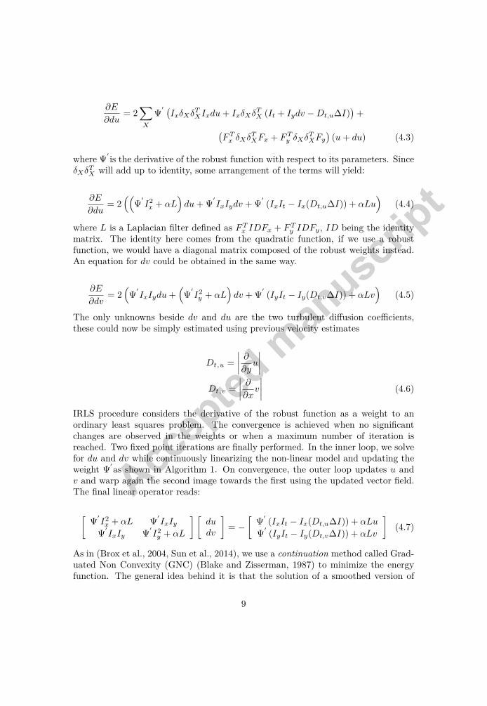
where Ψ′ is the derivative of the robust function with respect to its parameters. Since

δXδTX will add up to identity, some arrangement of the terms will yield:

∂E

∂du= 2

((Ψ

′I2x + αL

)du+Ψ

′IxIydv +Ψ

′(IxIt − Ix(Dt,u∆I)) + αLu

)(4.4)

where L is a Laplacian filter defined as FTx IDFx + FT

y IDFy, ID being the identitymatrix. The identity here comes from the quadratic function, if we use a robustfunction, we would have a diagonal matrix composed of the robust weights instead.An equation for dv could be obtained in the same way.

∂E

∂dv= 2

(Ψ

′IxIydu+

(Ψ

′I2y + αL

)dv +Ψ

′(IyIt − Iy(Dt,v∆I)) + αLv

)(4.5)

The only unknowns beside dv and du are the two turbulent diffusion coefficients,these could now be simply estimated using previous velocity estimates

Dt,u =

∣∣∣∣ ∂∂yu∣∣∣∣

Dt,v =

∣∣∣∣ ∂∂xv∣∣∣∣ (4.6)

IRLS procedure considers the derivative of the robust function as a weight to anordinary least squares problem. The convergence is achieved when no significantchanges are observed in the weights or when a maximum number of iteration isreached. Two fixed point iterations are finally performed. In the inner loop, we solvefor du and dv while continuously linearizing the non-linear model and updating theweight Ψ

′as shown in Algorithm 1. On convergence, the outer loop updates u andv and warp again the second image towards the first using the updated vector field.The final linear operator reads:

[Ψ

′I2x + αL Ψ

′IxIy

Ψ′IxIy Ψ

′I2y + αL

] [dudv

]= −

[Ψ

′(IxIt − Ix(Dt,u∆I)) + αLu

Ψ′(IyIt − Iy(Dt,v∆I)) + αLv

](4.7)

As in (Brox et al., 2004, Sun et al., 2014), we use a continuation method called Grad-uated Non Convexity (GNC) (Blake and Zisserman, 1987) to minimize the energyfunction. The general idea behind it is that the solution of a smoothed version of

9

Algorithm 1 Computation of optical flow on a pyramid level1: for i = 1 to the max number of warping steps do2: Compute Dt,u and Dt,v as in equation (4.6) using current u and v3: Warp the second image towards the first using current u and v.4: Initialize du , dv to zero5: for j = 1 to max number of linearization steps do6: Linearize the problem using equation (4.1)7: Compute the weight Ψ

′ .8: Solve for du and dv using equation (4.7)9: end for

10: update u and v using du and dv11: end for

the problem represents a good initialization to solve the original problem. In prac-tice, since we are dealing with a complicated optimization problem, the problem isfirstly convexified using the quadratic formulation and then it is linearly and grad-ually changed until the original problem formulation. The energy function to beminimized is obtained using:

cEQ + (1− c)ER (4.8)

where c ε [0, 1], EQ is the convex quadratic approximation of the problem, ER is therobust and possibly non convex original problem. The whole process is depicted inFigure (4.1).

10

Figure 4.1: A flowchart describing SGSD estimation cycle.

5. Evaluation

One of the key factors of the maturity of optical flow approaches ensues from theavailability of ground truth data. Authors compete in benchmarks such as Middle-bury (Baker et al., 2011) and MP Sintel (Butler et al., 2012) to evaluate their models.When optical flow was borrowed by experimental fluid dynamics community, similardatasets were required while considering the governing physics equations. A refer-ence simulation based on Navier-Stokes equations is used to generate such imagesusing the simulated (and hence, known) velocity fields (Carlier and Wieneke, 2005).For river sequences however, a 3D simulation that respects the physics of rivers andthen generate realistic 2D image sequences from it is a tedious job to do. Instead asimple idea has been utilized in this work to generate ground truth data. The ideais to track particles on Lagrangian basis throughout the sequence. First, a map ofreference trajectories is obtained by tracking these particles manually. The manualtracking is performed at pixel-level (after zooming) using CellTracker free software(Piccinini et al., 2016). The error related to manual selection depends on the qualityof the images. The error in the sequences we used in this study is about 1-2 pixelmaximum in the transverse direction. On the longitudinal direction, the error is 1-2pixels maximum for high quality images and 2-3 for degraded ones. Generally, weselect the brightest pixel within a group of pixels that forms the particle. Figure(5.1) shows the location of a chosen particle in the original image and the same par-ticle after zooming in two different images within the sequence. Then, integrating intime (through a 4th order Runge-Kutta), we reconstruct trajectories starting fromthe same initial points from the estimated displacement fields. The reconstructed

11

trajectories are then compared to their reference trajectories.

12

Figure 5.1: Manual tracking of particles: The position of the particle in the first image (top).Brightest position is chosen on pixel level after zooming in two different images (bottom).

13

We test the approach on different image sequences. The sequences differ mainlyin their displacement magnitude, image quality, density of tracers (if any) and sur-face perturbations. The reference trajectories were reconstructed up to few pixelsuncertainty. This is because particles change their orientations while moving andtheir form change as well when they are partially (or sometimes fully) occluded bywater. We compare our method SGSD to a modified (Horn and Schunck, 1981) vari-ation (HS). In fact, (HS) method used here is exactly the same as SGSD but doesnot include the turbulent diffusion term. A PIV-based method (Ray, 2011) that iscapable of producing dense vector fields (necessary for trajectory reconstruction) isalso compared to the two previous methods.

We use the same parameters for SGSD and for (HS) to highlight the difference ofresults with and without the diffusion term. Some of the aforementioned parametersare general and related to optical flow itself. For instance we use only two-stages GNCiterations in general. Additional GNC iterations improved the results for sequenceswith good seeding. Median filtering is another parameter to be considered. In generalit is well-suited for sequences with less turbulence. If applied to turbulent sequencesit might reject turbulent (but maybe correct) vectors and considers them as outliers.However, we found using it only between GNC iterations (and not between imagepyramids) to be beneficial in all cases. The weighting factor between the data termand the regularization term is chosen as 0.6 for all sequences. We found that ingeneral, the Lorentzian robust function works best for “good sequences”. For noisysequences or for those for which the 2D divergence assumption does not hold, the“Charbonnier” robust function (Charbonnier et al., 1994) gives slightly better resultsthan the Lorentzian. We compute the normalized distance error of trajectories ofdifferent methods and also for SGSD with different Sct values:

Error(i) =

√√√√√√((y(i)ref − y(i))

2+ (x(i)ref − x(i))

2)

√((y(1)ref − y(end)ref )

2+ (x(1)ref − x(end)ref )

2)

where ref subscript refers to a reference trajectory component. We chose to normal-ize the error because we have different displacement values for different sequences.Note that smaller value for Sct means larger diffusion coefficient and vice versa.We also exploit the dense nature of the estimation to compute relevant differentialoperators in a straightforward way.

5.1. Results on conventional imagesWe collect videos of rivers in motion from various sources like YouTube or from

research institutes data repositories. We require a fixed camera to make sure themotion is only due to the river. We also require the existence of at least few particlesfor the purpose of evaluation. The chosen particles are selected in such a way thatthey stay visible (at least partially) throughout the sequence.

14

5.1.1. The Arc river first sequenceThe Arc river, located in the french Alps, is known for its dark color water which

enhances the contrast (the gradient) of the image intensity when coupled with whitetracers. In addition, the image quality itself is good with no changes in scene lighting.The sequence has 41 images. The average displacement in the streamwise direction isapproximately 11 pixels between two images. In Figure (5.2), we plot the mean SGSDdense vector field (with an offset of few pixels for visualization purposes). This givesa quick spatio-temporal idea on the nature of the river at hand. Next, we plot thetrajectories of different methods along the reference trajectory. In Figure (5.3, top),it is easy to observe that all methods were generally in agreement with the referencetrajectory. This is mainly because of the good gradient signal in this sequence asmentioned earlier, but also to the quality of the images. Two zoomed areas aroundthe middle and the end of the trajectory are shown. SGSD is almost identical to thereference trajectory, followed by (HS) and then PIV which appears to underestimatethe motion magnitude. The zoomed window at the end of the trajectory confirms theresults on the zoomed window in the middle (any false positive match in the middlewill eventually result in a visible underestimation or overestimation in the window atthe end). The normalized distance error in Figure (5.3, middle) confirms the results.In Figure (5.3, bottom) we plot the normalized distance error of SGSD using differentvalues for Sct. This did not change the results much, there is a maximum error of0.015 for the case with no diffusion and around 0.05 for other cases with differentdiffusion coefficients. Still SGSD with Sct = 1 gives the best results. In Figure (5.4,left), we take advantage of the dense estimation to compute a fine-detailed divergencefield. In the same figure on the right, we could compute trajectories on an imagecross-section. Observe that these trajectories do not necessarily start at a particlelocation like the one in Figure (5.3, top). Nevertheless, they are consistent with eachother and specially to the ones that start at a particle location.

15

Figure 5.2: Mean dense SGSD velocity field of Arc river first sequence

16

Figure 5.3: The trajectories of different methods superimposed on the first image of Arc river firstsequence (top). Normalized distance error of different methods (middle). Normalized distance errorof SGSD with different turbulent Schmidt numbers (bottom)

17

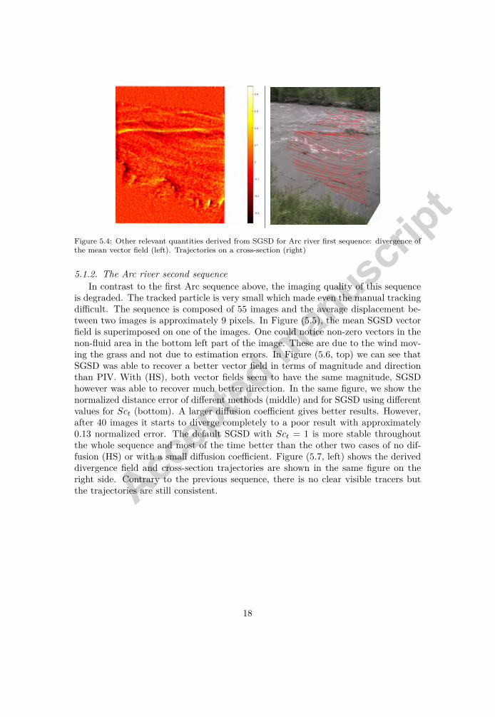
Figure 5.4: Other relevant quantities derived from SGSD for Arc river first sequence: divergence ofthe mean vector field (left). Trajectories on a cross-section (right)

5.1.2. The Arc river second sequenceIn contrast to the first Arc sequence above, the imaging quality of this sequence

is degraded. The tracked particle is very small which made even the manual trackingdifficult. The sequence is composed of 55 images and the average displacement be-tween two images is approximately 9 pixels. In Figure (5.5), the mean SGSD vectorfield is superimposed on one of the images. One could notice non-zero vectors in thenon-fluid area in the bottom left part of the image. These are due to the wind mov-ing the grass and not due to estimation errors. In Figure (5.6, top) we can see thatSGSD was able to recover a better vector field in terms of magnitude and directionthan PIV. With (HS), both vector fields seem to have the same magnitude, SGSDhowever was able to recover much better direction. In the same figure, we show thenormalized distance error of different methods (middle) and for SGSD using differentvalues for Sct (bottom). A larger diffusion coefficient gives better results. However,after 40 images it starts to diverge completely to a poor result with approximately0.13 normalized error. The default SGSD with Sct = 1 is more stable throughoutthe whole sequence and most of the time better than the other two cases of no dif-fusion (HS) or with a small diffusion coefficient. Figure (5.7, left) shows the deriveddivergence field and cross-section trajectories are shown in the same figure on theright side. Contrary to the previous sequence, there is no clear visible tracers butthe trajectories are still consistent.

18

Figure 5.5: Mean dense SGSD velocity field of Arc river second sequence

19

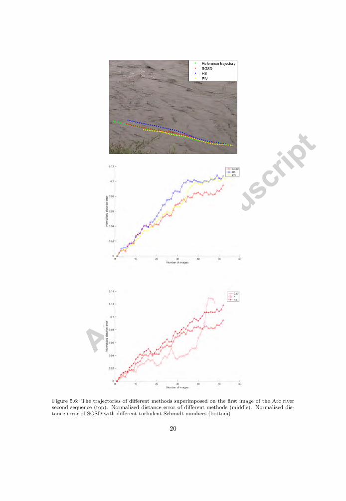
Figure 5.6: The trajectories of different methods superimposed on the first image of the Arc riversecond sequence (top). Normalized distance error of different methods (middle). Normalized dis-tance error of SGSD with different turbulent Schmidt numbers (bottom)

20

Figure 5.7: Other relevant quantities derived from SGSD for Arc river second sequence: divergenceof the mean vector field (left). Trajectories on a cross-section (right)

5.1.3. The Gave de Pau river sequenceThe Gave de Pau river, located in the french Pyrenees, is more challenging than

the previous cases. The sequence has many uniform regions with weak gradientsignal. Furthermore, the tracked particle is too big in size which increases the uncer-tainty of the reference trajectory reconstruction. This is because many pixels in thevicinity of the original selected pixel resemble each other. In addition, the river areawhere the particle resides (and a great deal of other parts) suffered from severe andpersistent 3D motion which causes the particle to move up and down for extendedperiod of time. This clearly violates the 2D incompressibility condition used to de-rive the optical flow model. The sequence is composed of 49 images with an averagedisplacement in the streamwise direction of approximately 6 pixels. In Figure (5.8),we get to have a general idea of the sequence motion patterns by plotting the meanSGSD vector field. The 3D deformations mentioned earlier are readily noticeablewhen visualizing the dense vector field. SGSD was able to recover a better trajectorycompared to other methods, Figure (5.9, top). Testing different Sct values otherthan the default value 1 showed similar performance for all variations until aroundthe 20th image where the default SGSD showed better performance while SGSD witha larger diffusion coefficient gives a trajectory that diverges drastically to a bad localminimum with approximately 0.5 normalized error, Figure (5.9, bottom). Figure(5.10, left) shows the divergence field and the cross-section trajectories are plottedon the right in the same figure. One could see the effect of the aforementioned 3Dmotion on the highlighted rectangular area plotted on the trajectories.

21

Figure 5.8: Mean dense SGSD velocity field of Gave de Pau sequence

22

Figure 5.9: The trajectories of different methods superimposed on the first image of Gave de Pauriver sequence (top), normalized distance error of different methods (middle) and the normalizeddistance error of SGSD with different turbulent Schmidt number (bottom)

23

Figure 5.10: Other relevant quantities derived from SGSD for Gave de Pau sequence: divergence ofthe mean vector field (left). Trajectories on a cross-section (right)

5.2. Results on ortho-rectified imagesIn river velocimetry, LSPIV is the benchmark image-based method to estimate

free surface velocity. It applies PIV to a grid of points defined in ortho-rectifiedimages. Image ortho-rectification is a way to transform the image to remove the per-spective effect so that a direct relationship between image space and the real worldcould be established, Figure (5.11). The resulting transformed sequence is used tocompute river velocity using image-based techniques like PIV. Unfortunately, the phi-losophy of LSPIV is different from optical flow which makes the comparison difficult.LSPIV relies on estimations obtained on many images and use statistics (the meanmostly) to average the final flow field to reduce the effects of outliers. This makestrajectory reconstruction difficult because it uses successive individual estimationsand only one outlier is enough to cause the whole trajectory to diverge. Optical flowis different in this regard as it integrates outlier rejection in the process (i.e. evenbetween only two images) via median filtering and/or regularization. In addition,the interpolation step needed for trajectory reconstruction will be more accurateon optical flow since the interpolation is applied between image pixels themselveswhile in LSPIV one needs to interpolate between grid points that are many pixelsapart, Figure(5.11, bottom). We used FUDAA-LSPIV software (Le Coz et al., 2014)to ortho-rectify the sequence and compute real world velocity on the defined grid.The sequence is extracted with 5 images per second frame-rate. We run SGSD onthe ortho-rectified sequence, Figure (5.12) shows SGSD trajectory reconstruction incomparison to the manual reference trajectory. To compare SGSD to LSPIV, wesuperimpose the same LSPIV grid on SGSD dense field and compare velocity valuesonly for grid points, Figure (5.13). Both methods give similar results. A noticeabledifference is observed on the top and bottom sides of the grid. However, this is notsurprising since estimations on image boundaries are known to be prone to errors. Inaddition, lower and upper part of images have no much tracers to rely on and theycontain a fixed shadow pattern.

24

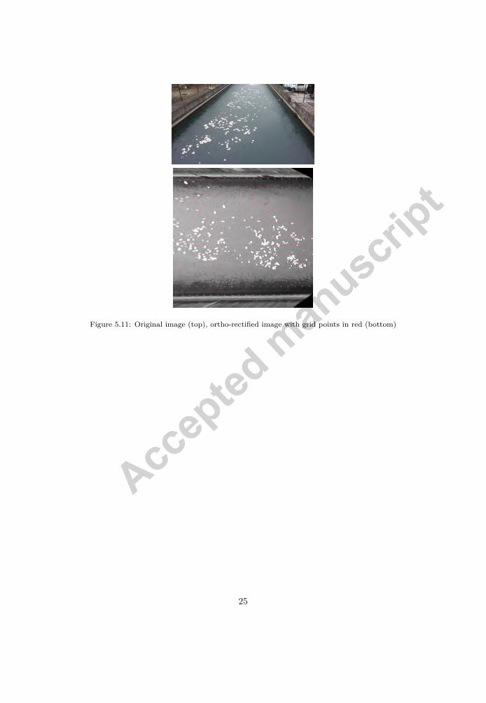
Figure 5.11: Original image (top), ortho-rectified image with grid points in red (bottom)

25

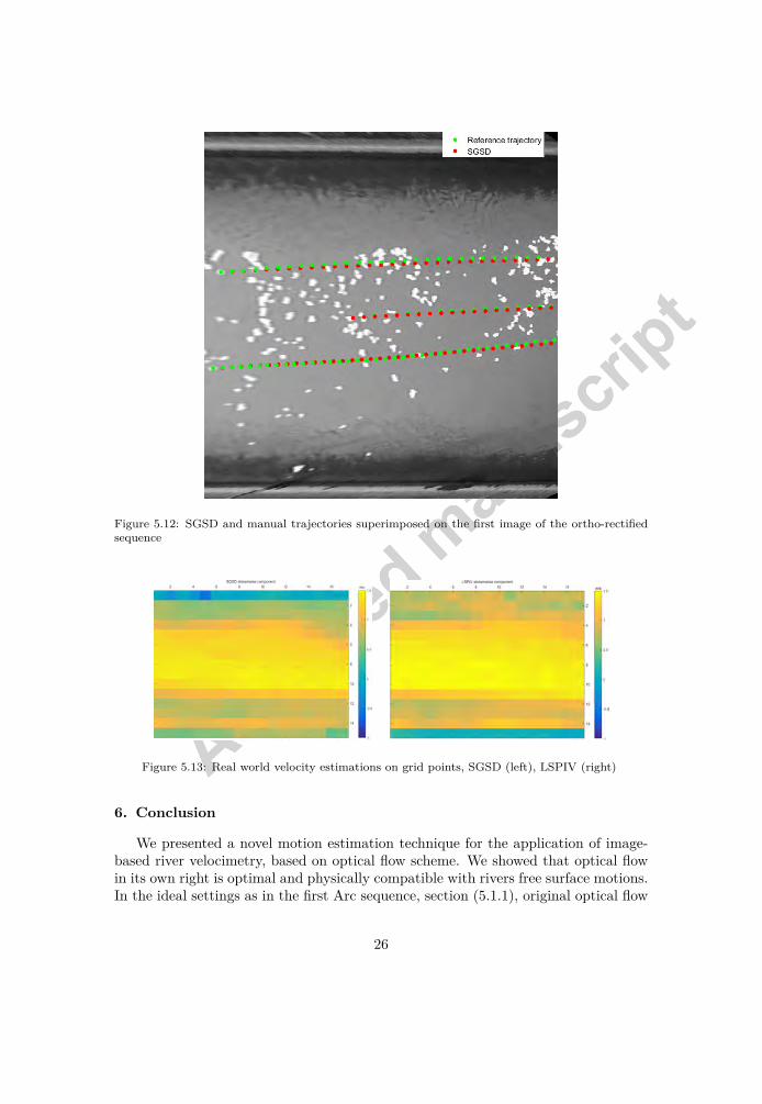
Figure 5.12: SGSD and manual trajectories superimposed on the first image of the ortho-rectifiedsequence

Figure 5.13: Real world velocity estimations on grid points, SGSD (left), LSPIV (right)

6. Conclusion

We presented a novel motion estimation technique for the application of image-based river velocimetry, based on optical flow scheme. We showed that optical flowin its own right is optimal and physically compatible with rivers free surface motions.In the ideal settings as in the first Arc sequence, section (5.1.1), original optical flow

26

provided very good results without any additional terms. Our enhanced model isbased on the decomposition of the scalar transport equation which is equivalent tothe original optical flow in addition to a new term. This term, considered to berelated to turbulent viscosity, models the small scale contributions that are droppedout in the image acquisition phase. We suggested a turbulent diffusion coefficientbased on Prandtl Mixing Length model and a Sct value of 1. This choice of Sct gavemore stable results. Other values (bigger or smaller than 1) either gave less accurateresults or good results at the beginning of the sequence but then drastically divergewith time. We presented results on different possible cases of rivers with or withouttracers, good or poor imaging conditions, high or low surface velocity and high orlow surface perturbations. Our method outperformed all other approaches in allimage sequences in the recovered motion magnitude and/or direction. Both assessedvisually or statistically via trajectory reconstruction of particles of interest. Wedraw the attention here to the sensibility of trajectory reconstruction to outliers, anywrong value at any instance of the estimated vector fields sequence will ruin the partof the trajectory that follows it. It is also sensitive to systematic errors that wouldaccumulate in time to reconstruct erroneous trajectories. Nevertheless, we have beenable to reconstruct trajectories that are similar to their reference trajectories. It isalso shown how the dense estimation of optical flow facilitates the computation ofother relevant quantities like divergence and vorticity fields. Since the applicationtreated here mainly focuses on river velocimetry, our model is designed to penalizethe vorticity of the vector field. However, the variational formulation is flexibleand could open the door to more specialized optical flow models for complex riverflows. In this case, new motion patterns will emerge that are different from thetranslatory pattern assumed in this paper. For example, a river flow around an objectwill introduce large-scale rotational motion pattern. The optical flow model couldbe easily changed to avoid the penalization of this quantity during the estimationprocess by using the regularization suggested by Chen et al. (2015). Using trajectoryreconstruction evaluation method feedback, new data terms/regularizers and modelsfor the diffusion coefficients could also be tested and assessed.

Acknowledgements

This work was supported by EDF-DTG and SCHAPI. Authors also would liketo thank Jérôme Le Coz and Alexandre Hauet for their insightful comments onFUDAA-LSPIV software along with the LSPIV project used in section 5.2.

Adrian, R., Jan. 1991. Particle-Imaging Techniques for Experimental Fluid-Mechanics. Annual Review of Fluid Mechanics 23 (1), 261–304.

Baker, S., Scharstein, D., Lewis, J. P., Roth, S., Black, M. J., Szeliski, R., Mar. 2011.A Database and Evaluation Methodology for Optical Flow. International Journalof Computer Vision 92 (1), 1–31.

27

Bergen, J. R., Anandan, P., Hanna, K. J., Hingorani, R., May 1992. HierarchicalModel-Based Motion Estimation. In: Computer Vision — ECCV 92. Springer,Berlin, Heidelberg, pp. 237–252.

Black, M. J., Anandan, P., Jan. 1996. The Robust Estimation of Multiple Motions:Parametric and Piecewise-Smooth Flow Fields. Computer Vision and Image Un-derstanding 63 (1), 75–104.

Blake, A., Zisserman, A., 1987. Visual Reconstruction. MIT Press.

Brox, T., Bruhn, A., Papenberg, N., Weickert, J., Jan. 2004. High Accuracy OpticalFlow Estimation Based on a Theory for Warping. In: Computer Vision - ECCV2004. Vol. 3024 of Lecture Notes in Computer Science. Springer Berlin Heidelberg,pp. 25–36.

Butler, D. J., Wulff, J., Stanley, G. B., Black, M. J., Oct. 2012. A Naturalistic OpenSource Movie for Optical Flow Evaluation. In: European Conf. on Computer Vision(ECCV). Part IV, LNCS 7577. Springer-Verlag, pp. 611–625.

Carlier, J., Wieneke, B., 2005. Report 1 on Production and Diffusion of Fluid Me-chanics Images and Data.

Cassisa, C., Simoens, S., Prinet, V., Shao, L., Dec. 2011. Subgrid Scale Formulationof Optical Flow for The Study of Turbulent Flow. Experiments in Fluids 51 (6),1739–1754.

Charbonnier, P., Blanc-Feraud, L., Aubert, G., Barlaud, M., Nov. 1994. Two De-terministic Half-Quadratic Regularization Algorithms for Computed Imaging. In:Proceedings of 1st International Conference on Image Processing. Vol. 2. pp.168–172 vol.2.

Chen, X., Zillé, P., Shao, L., Corpetti, T., Jan. 2015. Optical Flow for IncompressibleTurbulence Motion Estimation. Experiments in Fluids 56 (1).

Corpetti, T., Heitz, D., Arroyo, G., Mémin, E., Santa-Cruz, A., Oct. 2005. FluidExperimental Flow Estimation Based on an Optical-Flow Scheme. Experiments inFluids 40 (1), 80–97.

Cui, G. X., Xu, C. X., Fang, L., Shao, L., Zhang, Z. S., Jul. 2007. A New Sub-grid Eddy-Viscosity Model for Large-Eddy Simulation of Anisotropic Turbulence.Journal of Fluid Mechanics 582, 377–397.

Dramais, G., Le Coz, J., Camenen, B., Hauet, A., Dec. 2011. Advantages of a MobileLSPIV Method for Measuring Flood Discharges and Improving Stage-DischargeCurves. Journal of Hydro-environment Research 5 (4), 301–312.

Fujita, I., Muste, M., Kruger, A., 1998. Large-Scale Particle Image Velocimetryfor Flow Analysis in Hydraulic Engineering Applications. Journal of HydraulicResearch 36 (3), 397–414.

28

Gualtieri, C., Angeloudis, A., Bombardelli, F., Jha, S., Stoesser, T., Apr. 2017. Onthe Values for the Turbulent Schmidt Number in Environmental Flows. Fluids2 (2), 17.

Heitz, D., Héas, P., Mémin, E., Carlier, J., Oct. 2008. Dynamic ConsistentCorrelation-Variational Approach for Robust Optical Flow Estimation. Experi-ments in Fluids 45 (4), 595–608.

Heitz, D., Mémin, E., Schnörr, C., Mar. 2010. Variational Fluid Flow Measurementsfrom Image Sequences: Synopsis and Perspectives. Experiments in Fluids 48 (3),369–393.

Horn, B. K. P., Schunck, B. G., Aug. 1981. Determining Optical Flow. ArtificialIntelligence 17 (1–3), 185–203.

Jodeau, M., Hauet, A., Paquier, A., Coz, J. L., Dramais, G., 2008. Application andEvaluation of ls-piv Technique for the Monitoring of River Surface Velocities inHigh Flow Conditions. Flow Measurement and Instrumentation 19 (2), 117 – 127.

Khalid, M., Pénard, L., Mémin, E., Jul. 2017. Application of Optical Flow for RiverVelocimetry. In: 2017 IEEE International Geoscience and Remote Sensing Sym-posium. Fort-Worth, Texas, USA, pp. 6243–6246.

Le Coz, J., Jodeau, M., Hauet, A., Marchand, B., Le Boursicaud, R., 2014. Image-based Velocity and Discharge Measurements in Field and Laboratory River Engi-neering Studies Using the Free FUDAA-LSPIV Software. In: Proceedings of the In-ternational Conference on Fluvial Hydraulics, RIVER FLOW 2014. pp. 1961–1967.

Liu, C., Jun. 2009. Beyond Pixels: Exploring New Representations and Applicationsfor Motion Analysis. Ph.D. thesis, Massachusetts Institute of Technology.

Liu, T., Shen, L., Nov. 2008. Fluid Flow And Optical Flow. Journal of Fluid Me-chanics 614, 253–291.

Mémin, E., Pérez, P., Jan. 1998. A Multigrid Approach for Hierarchical MotionEstimation. In: Sixth International Conference on Computer Vision, 1998. pp.933–938.

Mémin, E., Pérez, P., Feb. 2002. Hierarchical Estimation and Segmentation of DenseMotion Fields. International Journal of Computer Vision 46 (2), 129–155.

Muste, M., Hauet, A., Fujita, I., Legout, C., Ho, H.-C., 2014. Capabilities of Large-Scale Particle Image Velocimetry to Characterize Shallow Free-Surface Flows. Ad-vances in Water Resources 70, 160 – 171.

Patalano, A., Garc C. M., Rodrez, A., 2017. Rectification of image velocity results(RIVeR): A simple and user-friendly toolbox for large scale water surface particleimage velocimetry (PIV) and particle tracking velocimetry (PTV). Computers &Geosciences 109, 323 – 330.

29

Piccinini, F., Kiss, A., Horvath, P., Mar. 2016. CellTracker (not only) for dummies.Bioinformatics 32 (6), 955–957.

Prandtl, L., 1925. Z. angew. Math. Mech. 5 (1), 136–139.

Ray, N., Oct. 2011. Computation of Fluid and Particle Motion From a Time-Sequenced Image Pair: A Global Outlier Identification Approach. IEEE Trans-actions on Image Processing 20 (10), 2925–2936.

Sun, D., Roth, S., Black, M., 2014. A Quantitative Analysis of Current Practices inOptical Flow Estimation and the Principles Behind Them. International Journalof Computer Vision 106 (2), 115–137.

Suter, D., Jun. 1994. Motion Estimation and Vector Splines. In: , 1994 IEEE Com-puter Society Conference on Computer Vision and Pattern Recognition, 1994.Proceedings CVPR ’94. pp. 939–942.

Tominaga, Y., Stathopoulos, T., 2007. Turbulent Schmidt Numbers for CFD Analysiswith Various Types of Flowfield. Atmospheric Environment 41 (37), 8091 – 8099.

30