OPTICAL COMMUNICATIONS - Lakehead...

Engineering 0550

OPTICAL COMMUNICATIONS

Laboratory Manual

Jason Servais El. Eng. Technologist

Department of Electrical Engineering

Lakehead University

Thunder Bay, ON

Winter 2009

THINK SAFETY

OPTICAL COMMUNICATIONS

3

Content Policy and Rules for Lab Exercises 4

Exp. #1 Part A − Linear Attenuation 6

Part B − Numerical Aperture 11

Part C − Misalignment Losses 16 Exp. #2 Propagation Modes 27 Exp. #3 Fiber Splicing 41 Appendix Technical Data 45

4 Lakehead University

Department of Electrical Engineering

POLICY AND RULES FOR LABORATORY EXERCISES

• No Food, No Beverages allowed in the laboratory room!!

• Keep clothes, bags, etc. OFF the benches with equipment on them.

• Be On Time ! Being late is annoying to your lab partners and if the experiment has progressed too far

you may not be credited with doing the experiment!

• Safety precautions must be observed at all times to prevent electric shock, damage to instruments, etc.

COME PREPARED! BOTH THE WRITTEN LAB REPORTS AND LAB PERFORMANCE (INCL. ATTITUDE,

PUNCTUALITY, PREPAREDNESS) WILL BE CONSIDERED FOR THE FINAL LAB MARK!

Lab Exercises

General

The maximum number of students in a lab work group is indicated on the sign-up sheet.

Should students leave a work group for whatever reason such that only one student remains in a group, this

student may join another team provided there is still room in that team without exceeding the above

maximum number.

Missed Lab Exercises

It is mandatory to perform all lab exercises according to course requirements.

Failure to perform one or more lab exercises results in a grade of "F" for the course.

When a student misses a lab exercise for whatever reason he/she must notify the instructor as soon as

possible. If the reasons given for the absence are satisfactory to the instructor, a make-up opportunity may

be arranged.

There may be a chance to let the student join another team to perform the missed lab provided this does not

then exceed the max number of students in that group. If it is not possible to accommodate this then a final

make-up date will be arranged to take place within one week after the end of classes. Should the student

fail to attend this appointment he/she will be required to provide sufficient proof of inability to attend

(medical certificate, air ticket, etc.) to avoid the "F" grade. The onus of proof lies entirely with the student!

The student then must immediately make another appointment with the lab instructor!

The lab report in such a case is due within one week after performance, else the "F' stands.

Lab Reports

General

It is mandatory that all lab reports must be submitted on time as specified by the lab instructor!

Plagiarism

Plagiarism will not be tolerated and may result in a grade of "F" for the course.

Any material taken from sources like books, manuals, web sites, magazines, etc. must be clearly referenced

as a footnote or under a bibliography!

A re-write of a report will be granted only under exceptional circumstances!

Missed Lab exercises

In some courses group lab reports may be allowed by the lab instructor. The group's composition is also

determined by the lab instructor.

If a student fails to perform a lab exercise with his group he/she will have to write his/her own individual

lab report!

Late Submission

The submission schedule (due date) will be made known by the attending lab instructor.

Late submission results in a deduction of 0.5 marks per day out of 10 full marks.

No or Partial Submission

A final date for submission will be clearly indicated on the sign-up sheet and/or announced by the lab

instructor. If after that date not all lab reports have been submitted, the student will receive a grade of "F"

for the course!

The deduction of marks for late submission still applies.

Format 5

• The report must be typed. Graphs may be produced by computer, provided the software is suited for

that use, i.e. grid, proper scaling and correct labelling can be achieved and the plot is smooth. If a

graph is used to extract data or to provide some precise information, show precisely how the

information is obtained (here it may be better to draw it on graph paper by hand - usually is faster, too).

• For your report use YOUR OWN words to present your report concise, clear and clean.

As pointed out above, copying etc. will be considered as plagiarism and will be severely punished

by reducing marks or, in severe cases, served with an "F" as mentioned above (the

provider/lender of the original work included)!

• The notes/sheets containing the raw data taken by each student during the experiment are to be

initialized by the attending technologist before leaving the lab and attached to the written report.

Reports with the raw data missing are subject to a deduction of one full mark (= 10%)!

The student is encouraged to develop and use his/her own personal style for writing and presenting

his/her report. However, standard procedures in industry and research laboratories require certain

information to be documented. Therefore, adhere fairly loosely to a general format like the following:

- Title page

(Please make an exception here: Pages stapled - no folders, plastic covers, etc):

Course number, Experiment number, Experiment Title, Name, Lab partners, Date of

performance

- Abstract

Statement of objective of the experiment (one or two sentences)

Concise and pertinent outline of the theory underlying the experiment (max one page)

- Experiment and Analysis

If the experiment consists of two or more parts, keep the experimental and analysis

sections together – the reader of your report does not want to continuously flip pages

back and forth to look for data etc.!

Brief outline of the method of investigation (whatever is applicable):

Procedure

Measurement techniques

Schematic diagrams

Equipment identification

Data (tables)

Observations relevant to the experiment and the results

Arrange experimental data, and do the necessary calculations (if applicable, at least a

sample calculation), to prepare for analysis

Theoretical calculations (at least sample calculation)

Comparison of experimental results with theory (preferably in form of tables/graphs)

Probable causes and magnitude of errors

- Conclusion (Summary)

- Review questions

- Raw data notes, attached to report, and initialized by the attending lab technologist.

GOOD PRESENTATION IS OF THE UTMOST IMPORTANCE, AS IS CORRECT ENGLISH AND GRAMMAR. EXPECT

20% OF YOUR LAB MARK ASSIGNED TO THIS AREA!!

GENERAL INFORMATION

EQUIPMENT

If equipment needs to be signed out, contact one of the technologists. The person signing it out is

responsible for it! Your marks will be held back until all equipment, books, data manuals, tools etc. are

returned (i.e. your graduation might depend upon it!).

Signed-out equipment has to be returned to the same technologist from whom you signed it out!

Assure your name is then removed from his sign-out list!

No equipment may be removed from any of the laboratories without explicit permission!

As you see, this is very important! TAKE LABS VERY SERIOUSLY! Lakehead University, Electrical Engineering Department July 2007

COMMUNICATIONS 1

Experiment No. 1 - 0550 Part A - Linear Attenuation

6

Part A : LINEAR ATTENUATION Abstracted from "Experiments in Fiber Optics", an instruction manual to accompany the KOP-200 fiber-optic experiments kit, by Pocatec Ltd., 2nd edition, P/N 3040107.

Objective To determine the linear attenuation of an optical fiber at various wavelengths.

Theory From the user point of view, one of the most important characteristics of the optical fiber is the attenuation of the transmitted signal as a function of the distance travelled in the fiber. This attenuation is mostly due to the intrinsic losses in the dielectric itself and to the microscopic irregularities at the core-cladding interface. The intrinsic losses are caused by the diffusion of light and by the absorption due ti impurities (OH and metallic ions). The attenuation of transmitted optical power depends also on the wavelength of the injected light as described by Raleigh's Law. However, the object of this investigation is the dependence of loss on the length of the fiber.

Figure 1-A1 To study the attenuation of an optical fiber, let us consider the model shown in Fig. 1-A1.

Let P(x) be the incident optical power and ∆x an infinitesimal length of fiber. The number

of photons diffused and absorbed is statistical and is proportional to P(x) and ∆x. Thus ( ) xxPP ∆−=∆ α

where α is a proportionality constant.

COMMUNICATIONS 1


7

This equation allows the writing of a relationship expressing the transmitted power versus the distance travelled in the fiber:

( )xPdx

dPα−=

( ) ( ) [ ]LePLP α−= 0 eq.(1)

where L is the total fiber length and P(0) the power injected at the fiber input. The

coefficient α represents the total attenuation and is evaluated in m−1 units. This expression plots a straight line on semilog paper.

Experiment

Equipment

KOP-200 fiber optic kit, Pocatec Ltd. Experimental Method

To determine the linear attenuation characteristics of a fiber, the method consists in injecting a constant level of optical power at a constant wavelength in fibers with different lengths and in measuring the corresponding transmitted power. A diagram of the relative

transmitted power as a function of fiber length allows the calculation of the α coefficient value and of the linear attenuation factor A in dB/m. One can write eq.(1) in logarithmic form as ( ) ( ) eLPLP 101010 log0loglog α−=

( ) LP α434.010log10 −=

where log P(0) is the ordinate for L=0 and 0.434α the slope. This plots a straight line on linear coordinate paper. The pre-amp output on the KOP-200 is an electrical signal V(L) proportional to the optical power P(L) incident on the PIN diode so that: ( )

( )( )

( )( )0

100

0

10 log434.0logLP

LPLL

LV

LV i

i

i ≡−= α

and ( )

( )( )

( )( )

( )i

i

i

i

LL

LP

LP

LL

LV

LV

−=

−=

0

0

10

0

0

10 loglog

434.0 α

eq.(2)

where V(Li) is the amplitude of the signal corresponding to length Li (i = 0,0.5,1,2,...).

COMMUNICATIONS 1


8

VLo is taken as the reference signal with L = 0, or very short (in our case the fiber F0.1 with 10cm length) and VLi with 0.5m, 1m etc. fiber lengths. By definition, linear attenuation A in dB/m is

( )

( )( )

( )α34.4

log10

/12

2

110

=−

=LL

LP

LP

mdBA

eq.(3)

where α is the total absorption coefficient in m−1.

Figure 1-A2 Test System Procedure

Note: Whenever possible, this experiment should be conducted in a dark room to minimize errors due to parasitic light.

(1) Linear Attenuation Measurement at 660nm See figures 1-A2 and 1-A3.

Set the MOD.-DIR. Switch on the electronics module at DIR and set GAIN at X1. Turn the KOP module on. Connect the red LED to the EMITTER output and the PIN photodiode to the PIN input. Connect the F0.1 fiber between the photo detector and source. Measure the output voltage, which is proportional to the input power. This is to be considered the power of the source and is the reference power level for the following measurements. The voltage should be at approx. 8.5…9V (above this level the diode may saturate).

COMMUNICATIONS 1


9

Replace F0.1 with the 0.5, 1, 2, 4, 6 and 8m fibers respectively and note the corresponding output amplitudes. Note: The attenuation (loss) coefficient can be greater for short distances where higher modes are attenuated more quickly.

(2) Linear Attenuation Measurement at 940nm Repeat the above measurements with the infrared LED.

Analysis Plot the readings on a semi-log chart. Linear scale: fiber length; log scale: signal amplitude. Determine the fiber linear attenuation factor in dB/m.

Conclusions Comment on your experiment.

COMMUNICATIONS 1


10

Figure 1-A3

COMMUNICATIONS 1

Experiment No. 1 - 0550 Part B - Numerical Aperture

11

Part B : NUMERICAL APERTURE Abstracted from "Experiments in Fiber Optics", an instruction manual to accompany the KOP-200 fiber-optic experiments kit, by Pocatec Ltd., 2nd edition, P/N 3040107.

Objective To determine the numerical aperture of a fiber by tracing the angular radiation pattern.

Theory When a ray of light inside a fiber core strikes the outside wall of the fiber at an angle of

incidence (to the fiber axis) less than the critical angle θc it will be totally internally reflected and contribute to the propagation of light along the fiber. If it strikes at greater than the critical angle some or all of the light will be refracted into the cladding material and be lost.

Figure 1-B1

At the critical angle θc, the ray will enter the cladding at an angle of 00, or parallel to the interface. Substituting this limit in Snell's Law give the critical angle as

CC nn θθ 2

12 sin1/cos −== eq.(4)

where n1 and n2 are the indices of refraction of the core and the cladding respectively. When the light is launched into a properly cut normal fiber end, it also experiences refraction at the air/core interface. Applying Snell's Law to this interface with the critical

angle ray gives a critical entry angle θa (to the fiber axis) where any rays with entry

COMMUNICATIONS 1


12

angles less than this critical angle value will propagate while those greater will not propagate. The critical entry angle is found to be

Ca nn θθ sinsin 10 = eq.(5)

Substituting n0 = 1 for air (or other if launching from a different medium), and for sin θc from eq.(4) gives the 2

2

2

1sin nnNA a −== θ eq.(6)

Experiment

Equipment

KOP-200 fiber optic kit, Pocatec Ltd. Effective Equilibrium Aperture

The numerical aperture expressed in eq.(4) is a characteristic of the fiber itself. It is dictated by the fiber structure and determines the maximum number of propagation modes the fiber will support. Another numerical aperture number applies because of the coupling efficiency between the light source and the fiber input end. This is the LAUNCH (or INPUT) NUMERICAL APERTURE NA1. If the source is arranged so that it presents an effective emitting area at the fiber entrance which is smaller than the fiber core cross-section area then the launch numerical aperture is identical to the fiber numerical aperture in eq.(6). If the area is greater, then a coefficient of coupling proportional to the two areas applies. If the source is efficiently coupled, then all of the allowed modes will be energized equally. However, in practice even though all of the allowed modes are excited at the input, some of the higher order modes will be lost in transmission due to scattering , bends in the fiber, mode cross-coupling, etc. Most of this loss will occur in the first 50 meters. The remaining energy is contained in lower modes, giving the effect of a reduction in the input numerical aperture with length from the input value NA1 to a lower EFFECTIVE EQUILIBRIUM NUMERICAL APERTURE value NAeq after the 50m length. The equilibrium numerical aperture can be measured by measuring the output numerical aperture for several lengths of fiber and plotting NA0 vs. length (Fig. 1-B2). The output numerical aperture can be measured by plotting the radiation pattern around the output fiber end. Numerical Aperture is defined as the solid angle containing 90% of the power, so that a graphic integration of the resulting curve will yield the acceptance

angle θa enclosing that 90%. A conical radiation pattern is assumed (Fig. 1-B3).

COMMUNICATIONS 1


13

Figure 1-B2 Figure 1-B3 Procedure

See Figs. 1-B2, 1-B3 and 1-B4.

1. Set the MOD.-DIR. Switch at DIR. and GAIN at X10.

2. Connect the RED LED to the EMITTER output and the photodiode to the PIN input.

3. Install the PIN photodiode on the X-Y mechanical stage and screw the LED to the L

bracket mounted on the turntable. The L bracket should be mounted so that the LED faces the PIN detector and is in the axis of rotation. (Use the two forward attachment holes near the bend in the L-bracket.)

4. Adjust the X-Y mechanical stage so as to leave about 1 cm between the LED and PIN detector.

5. Set the variable DC supply at 5V (for max. intensity) and connect it to the EMITTER input. Turn the electronic module ON.

6. Adjust the height of the X-Y mechanical stage to get a maximum PREAMP output signal at ~00 rotation angle. Weak lighting is preferable. Optical zero is attained by disconnecting the emitter.

7. Observe the ROTATION output and the PREAMP output using the voltmeter. The rotation output is 10 mV/degree.

8. If the LED angular emission pattern were traced by recording the radiant intensity as

a function of the rotated angle. (−900 to +900), one would get the graph as shown in Fig. 1-B3. However, this has proven not to be exactly the case with this equipment due to irregular radiation patterns of the LED. The plot would show 'bumps' and the maximum off center. Thus, to reduce the error caused by this, measure the

COMMUNICATIONS 1


14

maximum output (approx. middle position), then rotate the table to one side until the output is reduced to 10% of the maximum output and read the angle position. Then rotate to the other side and do the same. The angle in question is then half the total angle measured this way.

9. This measurement is to be done with the F0.1, F4 and F8 fibers.

Analysis 1. Determine the fiber numerical aperture for the various fiber lengths using the method outline above. 2. Calculate the theoretical value of N.A. using the fiber specifications, from the data sheet in the appendix.

2

2

2

1 nn −

3. Compare the results and comment on the effect of refraction index and fiber length on the numerical aperture.


COMMUNICATIONS 1


15

Figure 1-B4

COMMUNICATIONS 1

Experiment No. 1 - 0550 Part C - Misalignment Losses

16

Part C : MISALIGNMENT LOSSES Abstracted from "Experiments in Fiber Optics", an instruction manual to accompany the KOP-200 fiber-optic experiments kit, by Pocatec Ltd., 2nd edition, P/N 3040107.

Objective To determine the connecting losses due to core-to-core separation, axial misalignment, and angular misalignment, at a fiber joint.

Theory

a) GAP LOSS (CORE SEPARATION) Consider a fiber characterized by its numerical aperture and a receiving fiber identical to the first of diameter "D" and with gap "d".

Figure 1-C1 Since the rigorous calculation is complex, we will rely instead on two approxomations: one for small gaps (d < D) and the other for large gaps (d >> D).

a) Case 1: d < D

Figure 1-C1 shows the extremely diffracted rays related to maximum entry angle θ (N.A.

- sin θa). A ring of light bounded by ray D/2 and D/2 + tanθMd will not be transmitted to the receiving fiber.

COMMUNICATIONS 1


17

Fig. 1-C2 The right-handed side of the figure shows that intensity diminishes toward the outside (penumbrtal area). At point A, the intensity is half what it would be with d=0. the power at

the fiber exit is I0πD2/4. The power lost (not injected) is therefore the ring power, i.e., an intensity at the centre of

this ring equal to 1/4 and a ring length of πD giving a power loss of dtgD aθπ4/1

Naturally, the error becomes significant for excessivbely large "d"s. Losses in dB will therefore be

−

=

4

44lg102

2

DI

dtgDID

I

Pa

dBπ

θππ

By dividing each member by I πD2 / 4, we obtain ( )/1lg10 dtgP adB θ−=

However, the detail of the shape of the fiber emission pattern influences the results, and we can introduce a fit coefficient k (on the order of 0.7 to 1) ( )DdtgkP adB /1lg10 θ−=

b) Case 2: d >> D

The illuminated surface at distance d is π/4 (D + 2 tg θa d)2.

The illuminated surface at zero distance is π/4 D2.

COMMUNICATIONS 1


18

The loss in dB is therefore

( )

+

−=

4

24lg10

2

2

D

dtgD

Pa

dBπ

θπ

+−=

D

dtgP adB θ21lg20

b) AXIAL MISALIGNMENT

Axial misalignment δ is the nonalignment of the axis of the two fibers to be connected. In order to calculate the losses due to axial misalignment, we suppose, in first approximation, that the transmitted power is proportional to the surface common to both fibers (Fig. 1-C3).

Figure 1-C3 In that case, we can show that the ratio of the common surface to total fiber surface is

−

−

=

2

1arccos2

DDDSCOM

δδδ

π

where D represents the fiber diameter. Losses in dB due to axial misalignment (Paxial) then become

COMAXIAL SP 10log10−=

COMMUNICATIONS 1


19

−

−

−=

2

10 1arccos2

log10DDD

δδδ

π

eq.(7)

It can readily be imagined that the loss rises rapidly with increasing δ. Fortunately, this attenuation can fairly easily be kept to a minimum by precicion connectors using vlever mechanical designs.

c) ANGULAR MISALIGNMENT Angular misalignment losses appear when the axis of the fibers to be connected make a

nonzero angle θ (Fig. 1-C4).

Figure 1-C4 This angle produces an artificial numerical aperture variation because some rays emanating from the source fiber impact the input of the second fiber at an angle greater

than θa (angle of numerical aperture). The source fiber exit solid angle is: ( )aθπ cos121 −=Ω

Ω1 = exited light power.

Figure 1-C5

The solid angle accepted by the receiving fiber will be limited to Ω2 where a first approximation gives:

COMMUNICATIONS 1


20

( )( )4/cos122 αθπ −−=Ω a

Ω2 = received light power.

θa = N.A.

α = bending angle. The factor 4 is due to the fact that the transmission loss occurs on only 1 side out of 4 approximately.

Figure 1-C6 The losses expressed in dB will therefore be: ( )( )

( )( )

−

−−−=

a

a

dBPθπ

αθπ

cos12

4/cos12lg10

or ( )

−

−−−=

a

a

dBPθ

αθ

cos1

4/cos1lg10

Experiment

Equipment

KOP-200 fiber optic kit, Pocatec Ltd. General Note

In principle, these experiments require very high precision and expensive mechanical instrumentation. However, with a bit of care, patience and methodology, it is possible to meet the educational objectives of these manipulations. However, to facilitate things, you can use two 2mm fibers; i.e. the 2mm pigtail and the 2mm extended fiber (a piece of fiber sticks out at the connector).

COMMUNICATIONS 1


21

a) Losses Due to Core Separartion (see Fig. 1-C7)

To determine the losses due to core separation, we place the transmitting and receiving fibers end to end, then we move them apart using a precision movement, thereby enabling us to measure the ratio of the power injected into the receiving fiber to the total power carried by the transmitting fiber. Set the MOD-DIR switch at DIR and GAIN at X1.

Connect the RED LED to the TRANSMISSION output and the pin photodiode

connector to the PIN input.

Connect the extended fiber (F extend 1) to the TRANSMISSION output with the extended end connected to the L-bracket on the turntable

Install the L-bracket on the turntable as shown below:

Figure 1-C7 L-bracket for the Core Separation Experiment

Connect the pigtail fiber (1 mm) to the detector mounted on the X-Y mechanical stage.

Adjust to bring both fibers face to face.

Connect the PREAMP output to the Voltmeter and fine-adjust the fibers face to face on the mechanical stage in order to have a maximum signal. Adjust in all three axes carefully.

Connect the TRANSLATION output to the Voltmeter. The distance is measured at 1V/cm. (Seen from the right end of the apparatus, a clockwise turn moves the X-Y stage away from the L-bracket).

Beginning with the fibers face to face (d=0), move the receiving fiber away and trace the curve of the power injected into the receiving fiber as a function of the fiber separation d. Take measurements from d=0 to d~1mm in steps of approximately 0.2mm (i.e. ~ 5 steps of approx. 20mV each).

COMMUNICATIONS 1


22

b) Losses Due to Axial Misalignment (see Fig. 1-C10)

To determine the losses due to axial misalignment, we place the transmitting fiber on a rotating platen and measure the power lost by the receiving fiber as a function of the axis

displacement δ.

The lateral displacement δ can be considered as being proportional to the angular

displacement α (which is actually measured) and

δ = L tanα (L = 8 mm)

Notice that the extinction points corresponds to δ = D. Mount the L-bracket in the same position as shown in (Fig. 1-C8).

Figure 1-C8 L-bracket mounting for Axial Misalignment

Once again, bring the two fibers face to face for maximum output. Connect the ROTATION output and trace the curve of the power injected into the receiving fiber as a function of the angle of rotation (10mV/degree). The distance between the turntable axis and the transmitting end of the fiber is approximately L = 8mm.

Since δmax = D = 1 mm, the angle α which the platen has to be rotated will be very small and somewhat difficult to measure. Try as best as you can to measure from 0 to ~7 degrees rotation in 4..5 steps.

c) Angular Misalignment (Fig. 1-C11)

To determine the losses due to angular misalignment, mount the L-bracket in the same position as shown in Fig. 1-C7:

L-bracket mounting for Angular Misalignment

COMMUNICATIONS 1


23

Again, bring the fibers face to face, and for angles from 00 to 300 measure the power lost by the receiving fiber in about 6 steps as a function of the rotated angle. Be very careful to keep the edge of the end of the extended fiber in the axis of rotation (adjust the L-bracket with its locking screws).

Analysis a) Core Separation

Compute the separation losses in dB from the measured data. Compute the separation losses in dB from theory for the same range of d as

used in the experiment. Plot separation losses Ps [dB] vs. separation ratio (d/D) for both the measured

and the theoretical data onto the same graph. b) Axial Misalignment

Compute the axial misalignment losses in dB from the measured data. Compute the axial misalignment losses in dB from theory for the same range of

δ as used in the experiment.

Plot axial misalignment losses PAxial [dB] vs. axial displacement ratio (δ/D) for both the measured and the theoretical data onto the same graph.

c) Angular Misalignment

Compute the angular misalignment losses in dB from the measured data. Compute the angular misalignment losses in dB from theory for the same range

of θ as used in the experiment.

Plot the angular misalignment losses PAng [dB] vs. alignment angle θa [deg] for both the measured and the theoretical data onto the same graph.


COMMUNICATIONS 1


24

Figure 1-C9

COMMUNICATIONS 1


25

Figure 1-C10

COMMUNICATIONS 1


26

Figure 1-C11 .

COMMUNICATIONS 1

Experiment No. 2 - 0550 Propagation Modes

27

PROPAGATION MODES Abstracted from "Experiments in Fiber Optics", an instruction manual to accompany the KOP-200 fiber-optic experiments kit, by Pocatec Ltd., 2nd edition, P/N 3040107.

Objective To study the electromagnetic wave propagation in a waveguide.

Theory Since an optical fiber is a waveguide within which a light wave propagates, we must study the problem of electromagnetic wave propagation in a waveguide. As already mentioned, the phenomenon of total reflection allows us to consider the core cladding interface as being a mirror. For that reason and by analogy, let us consider a metallic waveguide, tha walls of which are mirrors of electromagnetic waves at optical frequencies (= 5x1014 Hz). This simplified approach gives us a better understanding of the physical phenomenon of guided wave propagation as well as of its importanta parameters.

Waveguide Model Let us consider a guide built from two parallel and infinetly wide metallic planes separated by the distance a. Think of the source as being a vertical wire (S0) centered in

the guide and carrying an alternating current with a frequency of ω (Fig. 2-1). The + sign indicates an upward directed current.

Figure 2-1

COMMUNICATIONS 1


28

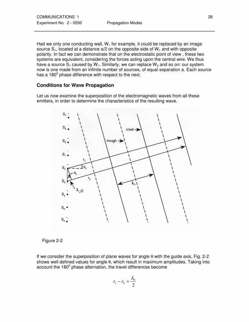
Had we only one conducting wall, W1 for example, it could be replaced by an image source S1, located at a distance a/2 on the opposite side of W1 and with opposite polarity. In fact we can demonstrate that on the electrostatic point of view , these two systems are equivalent, considering the forces acting upon the central wire. We thus have a source S1 caused by W1. Similarly, we can replace W2 and so on: our system now is one made from an infinite number of sources, of equal separation a. Each source has a 1800 phase difference with respect to the next.

Conditions for Wave Propagation Let us now examine the superposition of the electromagnetic waves from all these emitters, in order to determine the characteristics of the resulting wave.

Figure 2-2

If we consider the superposition of plane waves for angle θ with the guide axis, Fig. 2-2

shows well defined values for angle θ, which result in maximum amplitudes. Taking into account the 1800 phase alternation, the travel differences become

2

0

02

λ=− rr

COMMUNICATIONS 1


29

where

a2sin 0

0

λθ =

In general

( )2

12 0

12

λ+=− mrr

with

m = 0, ±1, ±2, ... and

( )a

mm2

12sin 0λθ +=

This expression may also be written as:

θ

λθ

cossin 0sS =

eq.(10)

with

s = ±1, ±3, ±5, ... In order to determine the resulting total amplitude within the guide, we must consider every image source shown in Fig. 2-3.

Figure 2-3

COMMUNICATIONS 1


30

At points A and C, we find two maxima which add and result in a maximum positive value. At point B we have two minima which result in maximum negative values. As time increases, points A, B, and C move along the guide symmetry axis. Distance AC corresponds to the wavelength of the lectromagnetic wave propagation in the guide. This

wavelength λg is related to wavelength λ0 by the following relationship:

θ

λλ

cos

0=g

eq.(11)

We have just demonstrated that, in metallic waveguide, there are well defined directions of propagation which correspond to different propagation conditions, the propagation

modes. We also found that the propagated wavelength, λg, is longer than the vacuum

wavelength λ0. The study of electromagnetic wave propagation in a plane wavelength, based on superpositions, is not the only sound approach used to determine the propagation conditioned. Let us consider a metallic waveguide where a plane wave propagates at

any angle θ with the guide axis as in Fig. 2-4. If the wave is to propagate in the guide, a ray of that wave will travel along the path AB to the wall of the guide where it experiences reflection. The reflected wave travels on until it encounters a second reflection at the other guide wall at C. The reflected wave will then travel along the path CD to the guide axis, in a line parallel to the original incident path AB to complete one full cycle of reflections. Figure 2-4 Calculation of Phase Difference between Reflected and Unreflected Waves in Guide

If the guide wall had not been present at B, then tie incident wave would have travelled along AB and continued in a straight line, arriiving at point E at an earlier time than the

COMMUNICATIONS 1


31

reflected wave will arrive at D. If propagation is to be supported at angle θ, then all points along wavefront 2 including E must have the same phase relation. If this is true, then the PHASE DIFFERENCE incurred along the two paths AE and AD must be an integer multiple of 2 radians, either positive or negative, or π2sir =Φ−Φ eq.(12)

where Φr represents the phase difference of the reflected wave

Φi represents the phase difference of the incident wave and

s = 0, ±1, ±2, ... When an electric wave encounters a reflection from a surface, it experiences a phase

delay of Φ = π radians, while a magnetic wave will experience a phase delay of Φ = 0. The total phase shift encountered by the unreflected wave in travelling from A to E is given by

( ) ( )

+=

=Φ

00

22

λ

π

λ

πBEABAEi

eq.(13)

The total phase shift encountered by the reflected wave in travelling from A to D is given by

( )

=Φ

0

2

λ

πADr

and thus

( ) Φ+

+++=Φ 2

2

0λ

πCDGCBGABr

eq.(14)

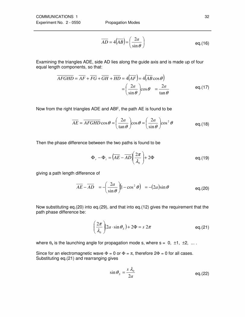
All of the path segment lengths may be restated in terms of the guide width a. Examining the diagram in Gig. 2-2, and noting the symmetry produced by the reflections, it is seen that the four triangles ABF, GBF, GCH, and DCH are right triangles identical in angle and height (a/2), so that the four path segments AB, BG, GC, and CE are of equal lengths. From triangle ABF this length is found to be:

θsin

2/aCEGCBGAB ====

eq.(15)

giving a total path length for the reflected wave from A to D of

COMMUNICATIONS 1


32

( )

==

θsin

24

aABAD

eq.(16)

Examining the triangles ADE, side AD lies along the guide axis and is made up of four equal length components, so that: ( ) ( )

θθ

θ

θ

tan

2cos

sin

2

cos44

aa

ABAFHDGHFGAFAFGHD

=

=

==+++=

eq.(17)

Now from the right triangles ADE and ABF, the path AE is found to be

θθ

θθ

θ 2cossin

2cos

tan

2cos

=

==

aaAFGHDAE

eq.(18)

Then the phase difference between the two paths is found to be

( ) Φ+

−=Φ−Φ 2

2

0λ

πADAEir

eq.(19)

giving a path length difference of

( ) ( ) θθθ

sin2cos1sin

2 2a

aADAE −=−

−=−

eq.(20)

Now substituting eq.(20) into eq.(29), and that into eq.(12) gives the requirement that the path phase difference be:

( ) πθλ

π22sin2

2

0

sa S =Φ+⋅

eq.(21)

where θs is the launching angle for propagation mode s, where s = 0, ±1, ±2, ... .

Since for an electromagnetic wave Φ = 0 or Φ = π, therefore 2Φ = 0 for all cases. Substituting eq.(21) and rearranging gives

a

sS

2sin 0λ

θ =

eq.(22)

COMMUNICATIONS 1


33

It should be noted that this expression allows both even and odd numbered modes while the previous result only allowed odd numbered modes. This latter method is less restrictive.

Dielectric Waveguide let us now consider a more realistic model of a fiber optic guide. This model uses two dielectric media with indexes n1 and n2. Let us determine the propagation conditions, using the demonstration from the preceding example. In order to simplify the problem, we shall consider a plane guide made from a dielectric slab of index n1 and thickness a. This first element is sandwiched between two dielectric slabs of index n2, lower than n1 (Fig. 2-5).

Figure 2-5

As before, let us consider a plane wave with an angle θ with the guide axis. we calculate

the phase differences between the incident wave (Φ1) and the reflected wave (Φr), taking into account the values of the refractive indexes. Obviously we suppose that the total

reflection condition is realized (cos θ > n2/n1). Consequently, we get eq.(18).

θθ

costan

2 01

=Φ

knai

eq.(23)

and

Φ+

=Φ 2

sin

2 01

θ

knar

eq.(24)

where the factor n1k0 accounts for the slower velocity of light in the dielectric slab with index of refraction n1. In that case, the solution of Fresnel's equations shows that for a transverse electric plane wave

COMMUNICATIONS 1


34

−

=Φ −

θ

θ

sin

cos

tan2

2

1

22

1n

n

eq.(25)

and as in the preceding case πmir 2=Φ−Φ

with m = 0, ±1, ±2, ... , so that eqs. (23), (24) and (25) allow the writing of

πθθθ

mkankan

2costan

22

sin

2 0101 =

−Φ+

πθ mkan 22sin2 01 =Φ+

θπ sin01kanm −=Φ

and

θπ

θ

θ

sin22sin

cos

tan 01

1

22

1kn

am

n

n

−=

−

−−

thus

θ

θπ

θsin

cos

2sin

2tan

2

1

22

01

−

=

−

n

n

mkna

eq.(26)

We must now consider separately the cases for odd and even values of m. A) Even values of m

m = 0, ±2, ±4, ±6, ...

COMMUNICATIONS 1


35

In this case, we get

θ

θ

θsin

cos

sin2

tan

2

1

22

01

−

=

n

n

kna

eq.(27)

To determine all allowed propagation modes, we only have to find the values for θ that satisfy eq. (27). For this purpose we define:

( ) ( )θθθ xkna

F tansin2

tan 011 =

=

eq.(28)

with

a = the thickness of the waveguide and k0 = 2π/λ0 and

( )θ

θ

θsin

cos

2

1

22

2

−

=n

n

F

eq.(29)

These two equations are transcendental, so we proceed numerically, or graphically by

tracing F1(θ) and F2(θ) vs. x(θ) to determine the intersection loci.

Example: We suppose

a = 10 µm n1 = 1.50

λ0 = 0.9µm n2 = 1.48

First, the maximum value for θ is found by zeroing function F2 :

F2(θmax) = 0 According to relationship eq.(29), we have

50.1

48.1cos

1

2max ==

n

nθ

and

θmax = 9.360

COMMUNICATIONS 1


36

This result is not surprising since it corresponds to the total reflection condition.

Then let us calculate the values for θ (θmax') that nullify function F1(θ) and trace F1(θ) and

F2(θ) vs. x(θ). After relationship eq.(28)

( ) πθθ 'sin2

'01 mkna

xm

==

in radians, with

m' = 0, ±1, ±2, ... and

01

'2'sin

Kan

mm

πθ =

1

0''sin

an

mm

λθ =

0

0

2

λ

π=K

Figure 2-6 The result of these calculations is presented in Fig. 2-6 and we can conclude that our guide can support only three propagation modes, those corresponding to even values of m. In general, since the number of modes (N1) corresponds to the number of times

functions F1(x(θ)) crosses the axis between x(θmax) > x(θ) > 0, therefore

( ) ( )πθθ 1sin2

1max01max −≥= Nkna

x

and

COMMUNICATIONS 1


37

0

max1

1

sin1

λ

θanN +≤

Introducing the numerical values from the example, we get N1 = 3.7, . . . and since we must take the smallest integer N1, the number of modes thus is three. B) Odd values of m

m = ±1, ±2, ±3, ... In this case, we get from eq.(26),

θ

θ

θsin

cos

sin2

cot

2

1

22

01

−

=

−

n

n

kna

and for the determining the different propagation modes, let us pose

( ) ( )θθθ xkna

F cotsin2

cot 013 −=

−=

eq.(30)

and we proceed graphically, tracing F2(θ) and F3(θ) to determine the intersection loci.

The values of θ that nullify the F3(θ) function correspond, in this case, to:

( )2

1'2'sin2

01

πθ += mkn

am

eq.(31)

with

m' = 0, ±1, ±2, ... and

1

0

2

1'sin

anmm

λ

+=

Considering the numerical values for the preceding example, we find three propagation modes corresponding to odd values of m (Fig. 2-7).

COMMUNICATIONS 1


38

Figure 2-7 As in the preceding case, since the number of odd modes (N2) corresponds to the

number of times function F3(x(θ)) crosses the axis between x(θmax) > x(θ) > 0, therefore

( )[ ]2

112sin2

2max01max

πθθ +−== Nkn

a

0

max1

2

sin

2

1

λ

θanN +≤

and obviously, we must take the next smallest integer. The total number of propagation modes supported by our plane guide, made from two dielectrics, then is the sum of integers N1 and N2. Since an actual optical waveguide is cylindrical and made from two dielectrics media, the exact conditions for guided propagation are more difficult to determine. The complete analysis of such a system requires an approach based upon the electromagnetic theory. Nevertheless, the analogies using the metallic parallel plate waveguide and the two-dielectric parallel plate guide model demonstrate well enough the principle of guided wave propagation and provide illustration for the different propagation modes.

COMMUNICATIONS 1


39

Experiment

Determination of the number of propagation modes, in a metallic waveguide model.

1. On a clear plastic sheet, trace a series of equally spaced parallel lines representing a

plane wave of wavelength λ0 (Fig. 2-8).

Figure 2-8

2. On a sheet of paper, trace two parallel lines representing a waveguide of width a =

2λ0 (Fig.2-9).

Figure 2-9

3. Put one plastic sheet over the paper and align a maximum over S0 and a minimum over S1. Determine, by moving (rotating) the transparency, the number of

propagation modes allowed by that waveguide and measure the corresponding θm.

4. On a second sheet of paper, trace two parallel lines representing a new guide of width

a' = 2a = 4λ0. Repeat steps 1 to 3.

COMMUNICATIONS 1


40

5. On a third transparency, trace a series of lines representing a plane wave of

wavelength λ'0 = λ0/2 and repeat the preceding example using the waveguide of

width a' = 2a. (This makes a'' = 8λ0). Repeat steps 1 to 3.

Analysis

For the three combinations, a=2λ0, a'=4λ0, and a''=8λ0, neatly table your results and compare to the values expected from eqs. (10) and (11).


Exercise 1 Consider a plane waveguide constituted of dielectric media where:

a = 10 µm n1 = 1.50 n2 = 1.49 λ0 = 633 nm (He-Ne laser wavelength). (a) Calculate the number of modes.

(b) For these conditions, trace functions F1(θ), F2(θ) and F3(θ) vs. x(θ) using eqs.(28), (29) and (30). Graphically determine the number of modes. (c) Change wavelength to 840 nm and calculate the number of modes. As above, graphically determine the number of modes.

(d) Change a to 100 µm and repeat the exercise using λ0 = 633 nm. (no graph required)

(e) Change n2 to 1.40 and repeat the exercise with λ0 = 633 nm and a = 100 µm. (no graph required) Comment.

Exercise 2 What is the condition required for having only one propagation mode?

Calculate ∆ = 1 − n2/n1 required at λ0 = 1.3 µm, n1 = 1.5, and a = 8µm.

COMMUNICATIONS 1

Experiment No. 3 - 0550 Fiber Splicing

41

FIBER SPLICING

ATTENTION

Be very careful !! Plastic coated fiber is very flexible, but when the coating is

removed the bare fiber breaks very easily and tiny glass chips may fly away,

especially when a fiber end is prepared by cleaving and breaking !

PLEASE do not touch or start experimenting before being instructed and having

attended a demonstration.

Objective To gain some hands-on experience in handling and splicing high quality optical fibers and measure the loss due to these splices.

Background Attaching optical fibers to connectors, adapters, other fibers, etc., is, of course, a necessity.

There are three common methods for attachments:

Fusion splicing

Elastomeric splicing

Using connectors

A large number of connectors are commercially available in varying qualities from simple to highly sophisticated connectors with losses from 2.5 dB to less than 1.0 dB.

Frequently there may be the need to keep the losses as low as possible. Then elastomeric or fusion splices will be preferred. In this experiment we will attempt to perform some of the latter splices.

The elastomeric splice uses a sleeve made of plastic into which the prepared ends are inserted. A small amount of optical index gel is applied to one of the fiber ends before insertion and one of the fibers is twisted slightly to achieve optimum power transfer. This splice will result in losses of less than 0.6 dB typical.

COMMUNICATIONS 1


42

In a fusion splice the ends of the two fibers have to be prepared and are then fused together with the aid of an arc welding process under a microscope. A good fusion splice will result in a loss of less than 0.1 dB typical.

In all cases, it is absolutely necessary to have the fiber ends properly prepared, that is, the end surface has to be plane, clean, devoid of all splits, cracks, etc. and in a right angle to the fiber axis.

Figure 3.1

Experiment

Equipment

Fusion Splicer (Power Technology) Fiber Optics Test Set (Photodyne) with source LED, 820nm Optical Variable Attenuator (Photodyne)

Fiber: type 150/50µm, 850nm Various tools for stripping the plastic coating and cleaving the fiber; connectors Microscope Procedure

Prepare the ends of several fibers until sufficient practice is gained to produce a satisfactory end surface. Usually fibers consist of the core, the plastic coating, sometimes a strength member, and the mantle. The fibers used here consist of core and coating only. First some length of plastic coating has to be removed, using a special stripping tool. Strip approx. 4 to 5 cm. The end surface of the core fibre most likely will be very rough. To get a clean surface the fiber is cleaved and broken. To remove any dirt and debris clean the end with acetone. Check the break under the microscope! Repeat the whole process if necessary . It will take some practice to accomplish a sufficiently clean break.

COMMUNICATIONS 1


43

(To reduce the losses of the fiber connection to a minimum the end surfaces used to be polished using a special polishing set. However, this is was a rather tedious and time-consuming procedure. Modern cleaving devices produce a clean break without the necessity for polishing) With a sufficient number of properly prepared ends of scrap fiber perform a few practice fusion splices. Proceed as shown by the lab instructor. Make sure the fiber ends are exactly aligned. The horizontal alignment can be observed directly looking into the microscope, to observe the vertical alignment the small mirror has to be flipped up. Having gained practice at making a satisfactory prepared fiber and splice , measure the loss of splices that you make, using the test loop shown below.

Figure 3.2 The Fiber Optics Test Set allows the uncomplicated measurement of splice losses in dB. A reference fiber is connected, and after pressing the blue "dB"-button, all following measurements give the difference in dB relative to the reference fiber. A source LED (820nm) is connected to the test set and the attenuator. The attenuator serves as an adaptor and to check on the continuity of the fiber but has no further significance for the measurement procedure. The fiber under test is then connected to the attenuator and the test set by means of adapters. Between attenuator and the spool a mode filter is inserted. Press the blue 'dB'-button, thus establishing a zero reference. Now break the fiber at a convenient place so that both ends again can be connected to the fusion splicer, and prepare the broken ends as practised. Fusion splice these ends together again. The reading indicates the loss due to the splice.

COMMUNICATIONS 1


44

Break the fiber twice again and fusion splice, taking readings as before. Average the three readings and compare your splice loss to the expected loss for fusion splices.

Report The report should describe the proceedings in your own words in short, but with all necessary details such that it can be used as a reference for yourself if you need to work with optical fibers at a later time.

COMMUNICATIONS 1

3 APPENDIX A

45

Appendix : TECHNICAL DATA

COMMUNICATIONS 1

3 APPENDIX A

46

COMMUNICATIONS 1

3 APPENDIX A

47

COMMUNICATIONS 1

3 APPENDIX A

48

OPTICAL COMMUNICATIONS - Lakehead...

Documents

Transcript of OPTICAL COMMUNICATIONS - Lakehead...