Optical and Thermodynamic properties of noble metal

nanoparticles. Effect of chemical functionalization.

Baudilio Tejerina and George C. Schatz

Objective

This laboratory is intended to introduce the student to the use of semiempirical electronic structure methods. In particular, the semiempirical methods will be applied to the study of metallic clusters and the interaction of the clusters with molecules such as pyridine. The reactivity of the metallic systems will be rationalized in terms of the electron populations in the cluster. Optical properties and the metal-ligand affinity will be quantitatively estimated.

Introduction • The noble metals nanoparticles (Cu, Ag and Au) exhibit physical properties that make them unique for scientific and technological applications: electronics, catalysis, biotechnology, spectroscopy, etc. These properties may be modulated by specific chemical treatment of the particles during their synthesis. Hence, the geometrical and electronic characterization of their structures is crucial to understand the mechanisms that control such properties.

• In this exercise, we will use a theoretical approach to study nanoparticles of Silver and Gold; including their structural and optical properties and the changes in these properties that arise from chemical functionalization. In order to assess the quality of our calculations it is common to contrast the results with other theoretical studies based on similar models.1 Thus, we will consider structures of tetrahedral/pyramidal shape whose geometries –interatomic distances and angles– have been taken from their natural crystal lattices.2

• The affinity of the metal particles for other chemical species will be calculated by the difference in energy between the isolated molecules and the aggregate. shows a schematic representation of the two binding modes of interaction between pyridine and a metal particle of pyramidal shape. With this schematic in mind, we will identify the reactive sites of the metal particles and study which mechanism is thermodynamically favored. The optical properties of different molecule-cluster systems will also be investigated.

Gold: Aikens, C. M.; Schatz, G. C. J. Phys. Chem, A 2006, 110, 13317. Silver: Zhao, L.; Jensen, L.; Schatz, G. C. J. Am. Chem. Soc. 2006, 128, 2911. Silver: Wyckoff, R. W. G. Crys. Struct. 1963, 1, 7. Gold: (a) Straumanis, M. E. Monatsh. Chem. 1971, 102, 1377. (b) Suh, I.-K.; Ohta, H.; Waseda. Y. J. Mater. Sci. 1988, 23, 757.

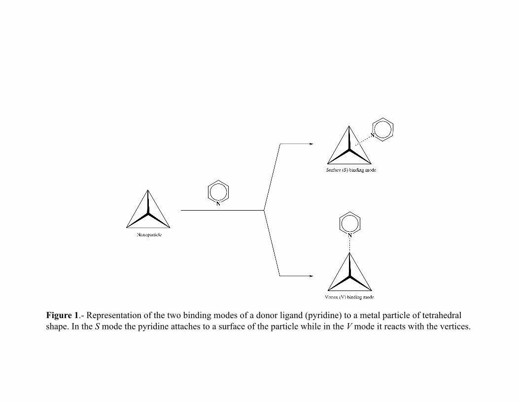
Figure 1.- Representation of the two binding modes of a donor ligand (pyridine) to a metal particle of tetrahedral shape. In the S mode the pyridine attaches to a surface of the particle while in the V mode it reacts with the vertices.

Procedure

For this particular exercise we will use the program CNDO/INDO accessible at the NanoHUB (www.nanohub.org). The atomic coordinates of the species that we will study are available on the class blackboard site (https://courses.northwestern.edu) in the folder named CA (Computer Assignments), subfolder NanoParticles.

NanoHUB - Log-in

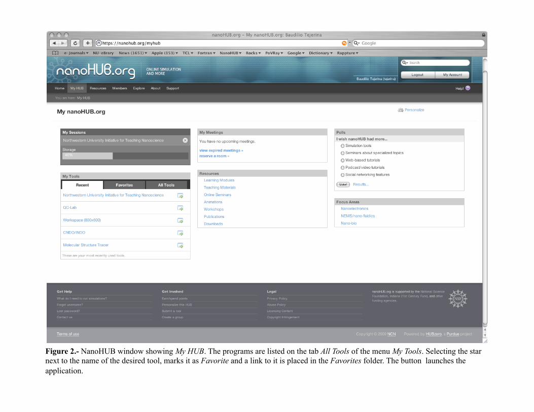
Figure 2.- NanoHUB window showing My HUB. The programs are listed on the tab All Tools of the menu My Tools. Selecting the star next to the name of the desired tool, marks it as Favorite and a link to it is placed in the Favorites folder. The button launches the application.

The CNDO/INDO program interface 1.- The CNDO/INDO program interface. After logging into the nanoHUB, select the option My HUB (see Figure2). On the menu My Tools select the tab All Tools and locate the application CNDO/INDO. If you click on the star next to the name, the application will be marked as Favorite and placed in the Favorites folder.3

At this point you may start the application by clicking on the Launch Tool button. The window with the program’s GUI will appear as illustrated in Figure 3. The Popout feature of the tool (located on the upper right hand side of the window) may be activated by clicking on the button; it will create a dedicated window to the tool on your local computer that facilitates the work.4

If you wish to continue working on the current project from a different location or computer, you may close the browser and even shut down the computer; when you log back into the NanoHUB all be as you left it. Even if a job was running, it will continue running on the background or, most likely, it will have finished the calculation in the meantime. Do not however click on the Close button, unless you wish to terminate the current CNDO/INDO session for good.

(3) Alternatively, you may call the program directly, www.nanohub.org/tools/cndo, or through the utility NUITNS (Northwestern University Initiative for Teaching NanoScience). The package NUITNS is located on www.nanohub.org/tools/nuitns and provides access to a group of complementary programs aimed to the study of molecular systems by electronic structure methods. (4) To reattach the window to the browser click again on the Popout button.

INDO/CNDO window

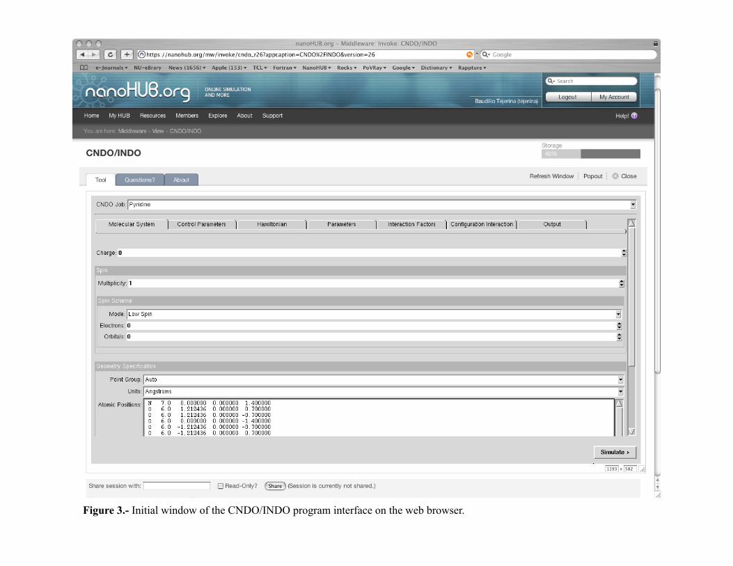
Figure 3.- Initial window of the CNDO/INDO program interface on the web browser.

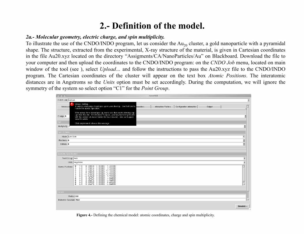
2.- Definition of the model. 2a.- Molecular geometry, electric charge, and spin multiplicity. To illustrate the use of the CNDO/INDO program, let us consider the Au20 cluster, a gold nanoparticle with a pyramidal shape. The structure, extracted from the experimental, X-ray structure of the material, is given in Cartesian coordinates in the file Au20.xyz located on the directory “Assigments/CA/NanoParticles/Au” on Blackboard. Download the file to your computer and then upload the coordinates to the CNDO/INDO program: on the CNDO Job menu, located on main window of the tool (see ), select Upload… and follow the instructions to pass the Au20.xyz file to the CNDO/INDO program. The Cartesian coordinates of the cluster will appear on the text box Atomic Positions. The interatomic distances are in Angstroms so the Units option must be set accordingly. During the computation, we will ignore the symmetry of the system so select option “C1” for the Point Group.

Figure 4.- Defining the chemical model: atomic coordinates, charge and spin multiplicity.

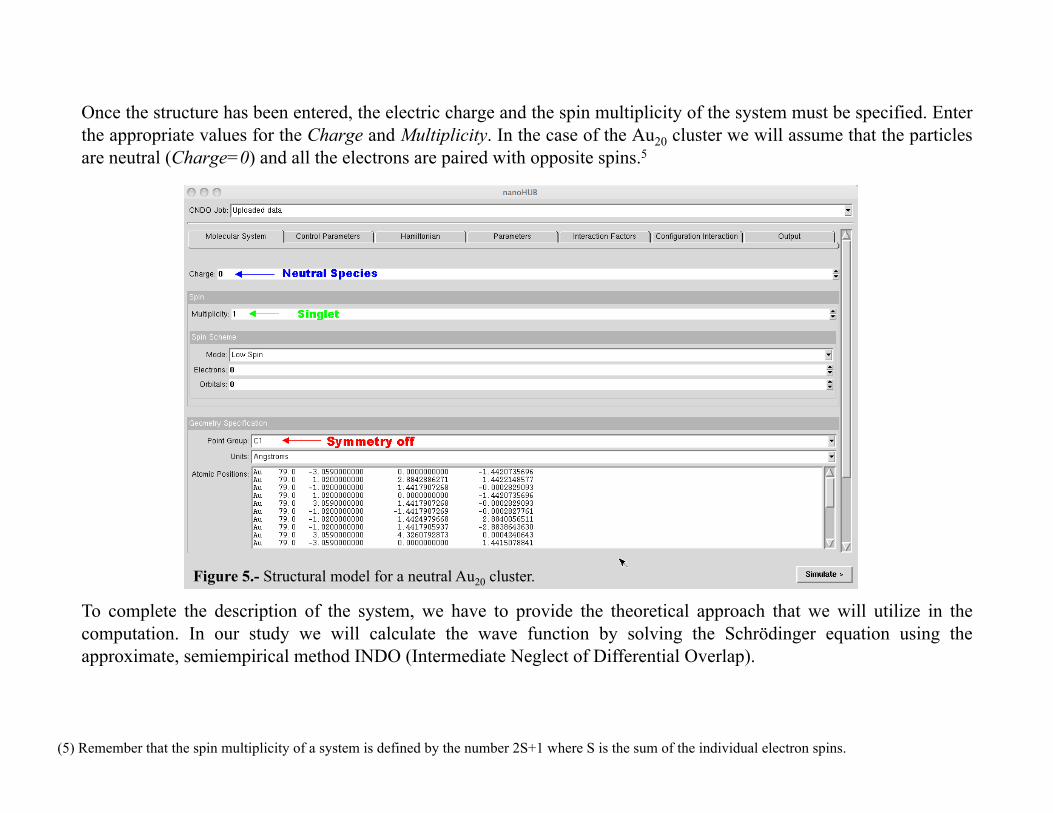
Once the structure has been entered, the electric charge and the spin multiplicity of the system must be specified. Enter the appropriate values for the Charge and Multiplicity. In the case of the Au20 cluster we will assume that the particles are neutral (Charge=0) and all the electrons are paired with opposite spins.5

(5) Remember that the spin multiplicity of a system is defined by the number 2S+1 where S is the sum of the individual electron spins.

Figure 5.- Structural model for a neutral Au20 cluster.

To complete the description of the system, we have to provide the theoretical approach that we will utilize in the computation. In our study we will calculate the wave function by solving the Schrödinger equation using the approximate, semiempirical method INDO (Intermediate Neglect of Differential Overlap).

2c.– Simulation parameters. The Schrödinger equation is solved iteratively using the SCF or Self-Consistent Field method. Figure 6 shows the parameters that control the calculation. In the SCF method, the wave function is recomputed cyclically until the associated energy converges that is, the difference in energy between two consecutive iterations drops below a predefined threshold. The limit is specified by the parameter Convergence in the Control Parameters tab. In this exercise, we will use 10-5 eV as the energy threshold and 200 SCF Iterations. This means that if the energy has not converged in 200 SCF iterations, the program will stop. It is a good practice to keep this parameter small, run the calculation and observe the SCF trend: if in the first few iterations it oscillates, stop the calculation and increase the SCF damping factor (Parameter Shift in Control Parameters). Then rerun the calculation. For small systems, the solution is generally found in fewer steps. If the SCF procedure is converging but it needs more iteration steps, it is possible to restart the calculation. See the section Restarting Computation.

Figure 6.- Simulation Control Parameters. The default values are appropriate for most of the calculations so in general they do not need to be changed.

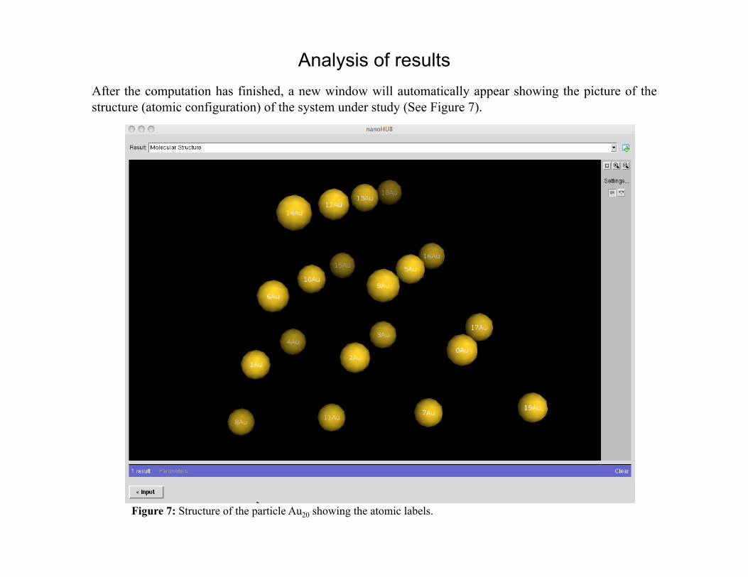
Analysis of results After the computation has finished, a new window will automatically appear showing the picture of the structure (atomic configuration) of the system under study (See Figure 7).

Figure 7: Structure of the particle Au20 showing the atomic labels.

Total Energy In order to verify that the calculation has been successfully completed we must make sure that the SCF procedure has converged. On the Result menu, select the option Output Log. The window contains the description of the system and the results of the calculation. You may either download its content to your local computer for further reference (advisable), or search for specific information on-line using the built-in ‘Find:’ button located at the lower part of the window. For instance, search for the text “total energy”; if the string is found, its first appearance will be highlighted (see Figure 8). In the example, the SCF took 10 iterations to find a solution for the semiempirical (INDO) Hartree-Fock equation. The total energy, sum of the electronic and nuclear energies, is –192.0721473 eV. A few lines below it is the energy that separates the highest occupied (HOMO) and lowest unoccupied (LUMO) molecular orbitals, 3.6775 eV.

Figure 8 Output Log showing the converged SCF total energy (highlighted) after 10 SCF cycles and the HOMO/LUMO energy gap, 3.6775 eV.

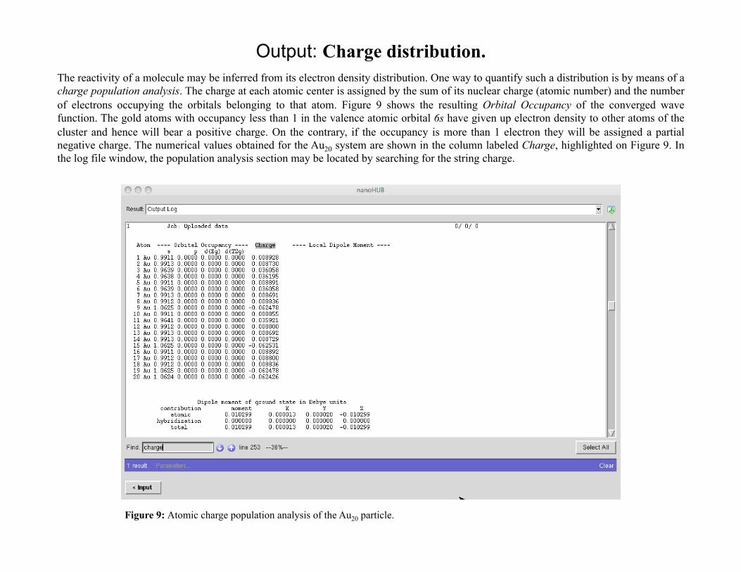
Output: Charge distribution. The reactivity of a molecule may be inferred from its electron density distribution. One way to quantify such a distribution is by means of a charge population analysis. The charge at each atomic center is assigned by the sum of its nuclear charge (atomic number) and the number of electrons occupying the orbitals belonging to that atom. Figure 9 shows the resulting Orbital Occupancy of the converged wave function. The gold atoms with occupancy less than 1 in the valence atomic orbital 6s have given up electron density to other atoms of the cluster and hence will bear a positive charge. On the contrary, if the occupancy is more than 1 electron they will be assigned a partial negative charge. The numerical values obtained for the Au20 system are shown in the column labeled Charge, highlighted on Figure 9. In the log file window, the population analysis section may be located by searching for the string charge.

Figure 9: Atomic charge population analysis of the Au20 particle.

Output: Charge distribution.

Based on the electron population analysis, we may define an electrostatic criterion to predict which centers in the Au20 will likely react with nucleophilic (e.g., positive Au atoms will attract nucleophilic ligands) species and which will react with electrophilic species. Although these electrostatic interactions may seem to be a reasonable argument to predict the initiating step of a reaction, it may not be sufficient, as electronic factors (i.e., which orbitals can combine to form bonds) are also in effect. Indeed electronic factors may dominate in the overall mechanism and change the direction of the reaction predicted by electrostatic factors alone. In a chemical process, the total energy is the factor that determines which product is more stable.

Output: Optical Properties. The absorption spectrum may be analyzed by reading the log file (search for the string wavelength), or with a tool that provides a graphical representation of this data showing the simulated UV/Vis spectrum as function of the wavelength. On the ‘Result’ options menu, select “Absorption spectrum”. The results obtained for the Au20 cluster are shown on Figure 10.

Figure 10: Calculated absorption spectrum of pyramidal, neutral Au20 particles.

Restarting current computation It is possible that the energy will not converge in the specified number of SCF iterations. In these cases, it is possible to restart and continue the calculation from the end of the previous one. To do so, first locate the SCF steps in the Output Log and make sure that the energy shows a convergent trend. Then, click on the Input button, which will take you back to the input window, and open the Control Parameters dialog tag as shown in Figure 11. On the Restart option select YES and for MO Assign pick PREVIOUS. At this point, the computation may be restarted by clicking on the Simulate button.

Figure 11: Restarting incomplete SCF calculations. Set Restart: YES and MO Assign: PREVIOUS.

Practice questions and exercises.

The Cartesian coordinates of the structures are available for download on ….??? (www.nanohub.org) somewhere.

A Nanoparticles (structure comparisons). 1.- Nucleation. The files M4_Tetrahedral.xyz and M4_Planar.xyz (with M= Ag and Au) contain the coordinates for the tetrahedral and planar M4 clusters, respectively. Using the semiempirical method INDO, calculate the electronic structures and tabulate the total energies of the clusters as a function of the geometry and the nature of the metal M.