OPRE 6201 : 4. Network Problems

1 The Transportation Problem

1.1 An LP Formulation

Suppose a company has m warehouses and n retail outlets. A single product is to be shipped from thewarehouses to the outlets. Each warehouse has a given level of supply, and each outlet has a given level ofdemand. We are also given the transportation costs between every pair of warehouse and outlet, and thesecosts are assumed to be linear. More explicitly, the assumptions are:

• The total supply of the product from warehouse i is ai, where i = 1, 2, . . ., m.

• The total demand for the product at outlet j is bj , where j = 1, 2, . . ., n.

• The cost of sending one unit of the product from warehouse i to outlet j is equal to cij , where i = 1,2, . . ., m and j = 1, 2, . . ., n. The total cost of a shipment is linear in the size of the shipment.

The problem of interest is to determine an optimal transportation scheme between the warehouses and theoutlets, subject to the specified supply and demand constraints. Graphically, a transportation problem isoften visualized as a network with m source nodes, n sink nodes, and a set of m · n “directed arcs.” This isdepicted in Figure 1. We now proceed with a linear-programming formulation of this problem.

1.2 The Decision Variables

A transportation scheme is a complete specification of how many units of the product should be shippedfrom each warehouse to each outlet. Therefore, the decision variables are:

xij = the size of the shipment from warehouse i to outlet j, where i = 1, 2, . . ., m and j = 1, 2, . . ., n.

This is a set of m · n variables.

1.3 The Objective Function

Consider the shipment from warehouse i to outlet j. For any i and any j, the transportation cost per unitis cij ; and the size of the shipment is xij . Since we assume that the cost function is linear, the total cost ofthis shipment is given by cijxij . Summing over all i and all j now yields the overall transportation cost forall warehouse-outlet combinations. That is, our objective function is:

Minimizem∑

i=1

n∑

j=1

cijxij .

1

Figure 1: A transportation network with m sources and n sinks.

1.4 The Constraints

Consider warehouse i. The total outgoing shipment from this warehouse is the sum xi1 + xi2 + · · · + xin.In summation notation, this is written as

∑nj=1 xij . Since the total supply from warehouse i is ai, the total

outgoing shipment cannot exceed ai. That is, we must require

n∑

j=1

xij ≤ ai , for i = 1, 2, . . . , m.

Consider outlet j. The total incoming shipment at this outlet is the sum x1j + x2j + · · · + xmj . Insummation notation, this is written as

∑mi=1 xij . Since the demand at outlet j is bj , the total incoming

shipment should not be less than bj . That is, we must require

m∑

i=1

xij ≥ bj , for j = 1, 2, . . . , n.

This results in a set of m + n functional constraints. Of course, as physical shipments, the xij ’s should benonnegative.

2

1.5 LP Formulation

In summary, we have arrived at the following formulation:

Minimizem∑

i=1

n∑

j=1

cijxij

Subject to:n∑

j=1

xij ≤ ai for i = 1, 2, . . . , m

m∑

i=1

xij ≥ bj for j = 1, 2, . . . , n

xij ≥ 0 for i = 1, 2, . . . , m and j = 1, 2, . . . , n.

This is a linear program with m ·n decision variables, m +n functional constraints, and m ·n nonnegativityconstraints.

1.6 A Numerical Example

In an actual instance of the transportation problem, we need to specify m and n, and replace the ai’s, thebj ’s, and the cij ’s with explicit numerical values. As a simple example, suppose we are given: m = 3 andn = 2; a1 = 45, a2 = 60, and a3 = 35; b1 = 50 and b2 = 60; and finally, c11 = 3, c12 = 2, c21 = 1, c22 = 5,c31 = 2, and c32 = 4. Then, substitution of these values into the above formulation leads to the followingexplicit problem:

Minimize 3x11 +2x12 +x21 +5x22 +2x31 +4x32

Subject to:x11 +x12 ≤ 45 (1)

x21 +x22 ≤ 60 (2)x31 +x32 ≤ 35 (3)

x11 +x21 +x31 ≥ 50 (4)x12 +x22 +x32 ≥ 60 (5)

xij ≥ 0 for i = 1, 2, 3 and j = 1, 2.

For an example of an explicit transportation scheme, let x11 = 20, x12 = 20, x21 = 20, x22 = 20,x31 = 10, and x32 = 20. It is easily seen that this proposed solution satisfies all of the constraints, and henceit is feasible. In words, the solution calls for shipping 20 units from warehouse 1 to outlet 1, 20 units fromwarehouse 1 to outlet 2, 20 units from warehouse 2 to outlet 1, . . ., and finally 20 units from warehouse 3to outlet 2. The total transportation cost associated with this transportation scheme can be computed as:

3 · 20 + 2 · 20 + 1 · 20 + 5 · 20 + 2 · 10 + 4 · 20 = 320.

1.7 An Equivalent Formulation

To derive an optimal transportation scheme for the above example, we can of course apply the standardSimplex algorithm. This means that we will first introduce 3 slack variables for constraints (1), (2), and (3)and 2 surplus variables for constraints (4) and (5), to convert these inequalities into equalities. On top ofthese, at the onset of Big-M, we also need to introduce 2 more artificial variables to serve as starting basicvariables for constraints (4) and (5). We would then go through Big-M procedure. This routine is standard,but the introduction of so many new variables seems tedious. Can we do better? It turns out that we can.

3

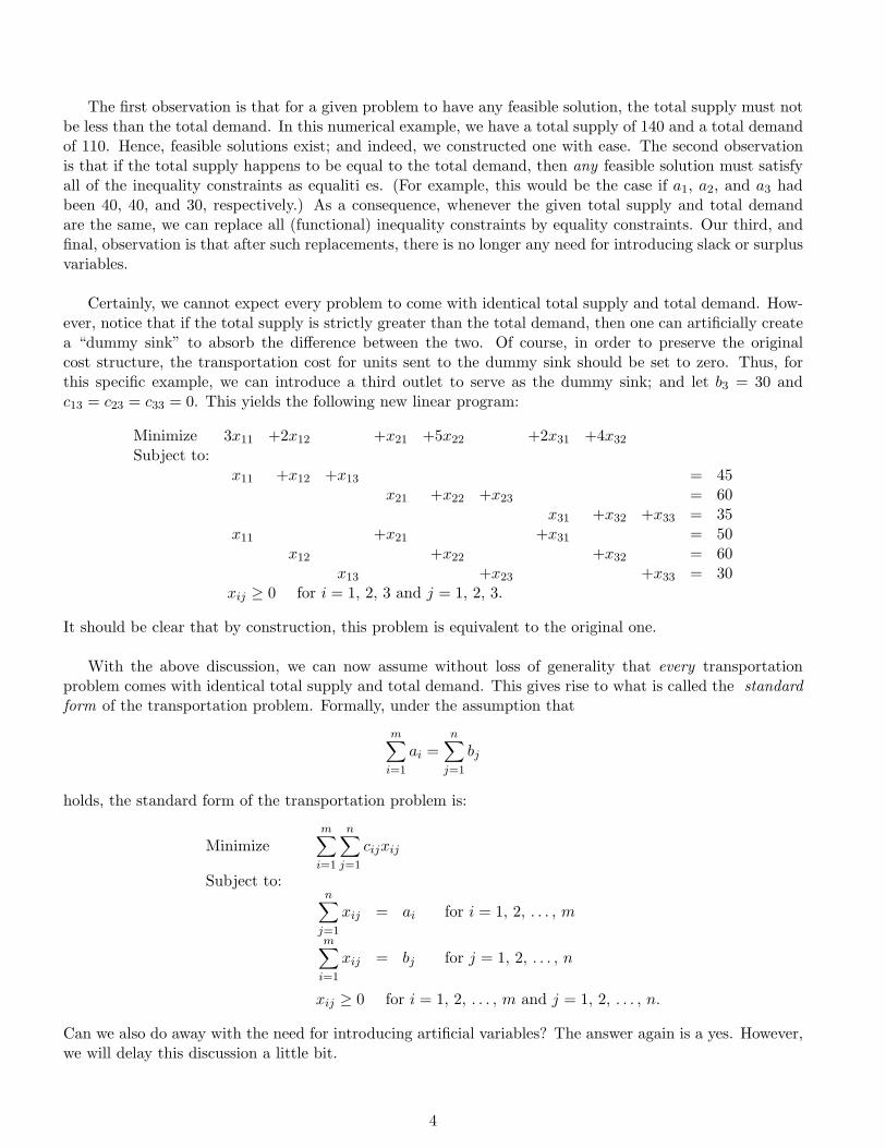
The first observation is that for a given problem to have any feasible solution, the total supply must notbe less than the total demand. In this numerical example, we have a total supply of 140 and a total demandof 110. Hence, feasible solutions exist; and indeed, we constructed one with ease. The second observationis that if the total supply happens to be equal to the total demand, then any feasible solution must satisfyall of the inequality constraints as equaliti es. (For example, this would be the case if a1, a2, and a3 hadbeen 40, 40, and 30, respectively.) As a consequence, whenever the given total supply and total demandare the same, we can replace all (functional) inequality constraints by equality constraints. Our third, andfinal, observation is that after such replacements, there is no longer any need for introducing slack or surplusvariables.

Certainly, we cannot expect every problem to come with identical total supply and total demand. How-ever, notice that if the total supply is strictly greater than the total demand, then one can artificially createa “dummy sink” to absorb the difference between the two. Of course, in order to preserve the originalcost structure, the transportation cost for units sent to the dummy sink should be set to zero. Thus, forthis specific example, we can introduce a third outlet to serve as the dummy sink; and let b3 = 30 andc13 = c23 = c33 = 0. This yields the following new linear program:

Minimize 3x11 +2x12 +x21 +5x22 +2x31 +4x32

Subject to:x11 +x12 +x13 = 45

x21 +x22 +x23 = 60x31 +x32 +x33 = 35

x11 +x21 +x31 = 50x12 +x22 +x32 = 60

x13 +x23 +x33 = 30xij ≥ 0 for i = 1, 2, 3 and j = 1, 2, 3.

It should be clear that by construction, this problem is equivalent to the original one.

With the above discussion, we can now assume without loss of generality that every transportationproblem comes with identical total supply and total demand. This gives rise to what is called the standardform of the transportation problem. Formally, under the assumption that

m∑

i=1

ai =n∑

j=1

bj

holds, the standard form of the transportation problem is:

Minimizem∑

i=1

n∑

j=1

cijxij

Subject to:n∑

j=1

xij = ai for i = 1, 2, . . . , m

m∑

i=1

xij = bj for j = 1, 2, . . . , n

xij ≥ 0 for i = 1, 2, . . . , m and j = 1, 2, . . . , n.

Can we also do away with the need for introducing artificial variables? The answer again is a yes. However,we will delay this discussion a little bit.

4

1.8 The Transportation Tableau

The Simplex tableau serves as a very compact format for representing and manipulating linear programs.In the same spirit, we now introduce a tableau representation for transportation problems that are in thestandard form.

For a problem with m sources and n sinks, the tableau will be a table with m rows and n columns.Specifically, each source will have a corresponding row; and each sink, a corresponding column. For ease ofreference, we shall refer to the cell that is located at the intersection of the ith row and the jth column as“cell (i, j)”. Parameters of the problem will be entered into various parts of the table in the format below.

Sink j......

cij

Source i · · · · · · xij · · · · · · ai......bj

That is, each row is labelled with its corresponding source name at the left margin; each column is labelledwith its corresponding sink name at the top margin; the supply from source i is listed at the right marginof the ith row; the demand at sink j is listed at the bottom margin of the jth column; the transportationcost cij is listed in a subcell located at the upper-left corner of cell (i, j); and finally, the value of xij is tobe entered at the lower-right corner of cell (i, j).

Again, we will use the numerical example above to illustrate the just-described format. With theintroduction of a dummy sink to balance the total supply and total demand, this problem has three sourcesand three sinks. Therefore, the parameters of the problem can be specified in the explicit 3 ·3 tableau below.

Sinks1 2 3

3 2 01 45

1 5 0Sources 2 60

5 4 03 35

50 60 30

Notice that we have left the spaces for the xij ’s blank; these will be filled in later, when we begin thesolution process. As a specific example, the feasible solution x11 = 20, x12 = 20, x13 = 5, x21 = 20,

5

x22 = 20, x23 = 20, x31 = 10, x32 = 20, and x33 = 5 would be entered as in the tableau below.

Sinks1 2 3

3 2 01 20 20 5 45

1 5 0Sources 2 20 20 20 60

5 4 03 10 20 5 35

50 60 30

All transportation problems in the standard form will henceforth be specified in this compact tableau format.

1.9 Remarks

1. In most applications, the shipments are integer-valued. We have ignored this requirement in ourformulation. However, it will turn out that if the specified ai’s and bj ’s are integers, then the optimalsolution of a transportation problem produced by the Simplex algorithm also is integer-valued.

2. In applications where an oversupply exists, it is often desirable to assume that there is an inventory-holding cost for units that are not shipped out. If this is the case, then we can easily accommodatethe inventory-holding costs as part of the objective function by reinterpreting them as transportationcosts to the dummy sink.

3. When the total supply is less than the total demand, it is still possible to create a balanced trans-portation problem. The idea is to create a dummy source and let it have a supply that equals thedifference between the total demand and the total supply. In doing so, it may be reasonable to assessa shortage penalty cost for units that are sent (fictitiously) from the dummy source to any sink.

2 Constructing an Initial Basic Feasible Solution

We will use the previous numerical example to illustrate the methods. In algebraic form, our problem is:

Minimize 3x11 +2x12 +x21 +5x22 +2x31 +4x32

Subject to:x11 +x12 +x13 = 45

x21 +x22 +x23 = 60x31 +x32 +x33 = 35

x11 +x21 +x31 = 50x12 +x22 +x32 = 60

x13 +x23 +x33 = 30

xij ≥ 0 for i = 1, 2, 3 and j = 1, 2, 3;

6

and in tableau form, this problem is specified as:

Sinks1 2 3

3 2 01 45

1 5 0Sources 2 60

5 4 03 35

50 60 30

An inspection of the algebraic form of the problem shows that we have a set of 6 equality constraints in 9variables. We will first argue that it is possible to reduce the number of constraint equations by 1. This is aconsequence of the following special feature of all balanced transportation problems. Notice that the threesupply constraints sum up to

x11 +x12 +x13 +x21 +x22 +x23 +x31 +x32 +x33 = 140 ;

and that the three demand constraints also sum up to this same expression. It follows that it is sufficientto work with any subset of 5 out of these 6 equations. To understand what this means more explicitly,suppose we are given a proposed solution to the original equations, and we are asked to check whether ornot the given solution is feasible. To answer this, we would have to substitute the proposed solution into theequations one by one. Now, observe that if the proposed solution is verified to satisfy the first 5 equations,then the equality of the sum of the supply equations and the sum of the demand equations implies thatthe proposed solution must also satisfy the last equation. Moreover, it should be clear that this observationholds regardless of the order in which the equations are checked. Thus, indeed, we can choose to removeany one of the given 6 equations, and doing so will not alter the feasible set in any way.

The next question of course is: Which equation should we remove? Interestingly, the answer is that wedon’t have to commit ourselves at this point. Intuitively, the reason behind this answer is that doing sowould give us more flexibility; this will be made more apparent a little bit later.

With one equation removed (conceptually, that is), a basic feasible solution will have 5 basic variablesand 4 nonbasic variables. If we are to solve this problem by the standard Simplex method, then our nexttask is to introduce 5 artificial variables (Actually, 4 is sufficient. Why?) and begin Phase I of the solutionprocedure. As noted earlier, it seems desirable to avoid introducing these additional variables (since we haveto drive them out of the basis eventually). We are, therefore, motivated to explore other, hopefully more-direct, approaches. For this purpose, we will now switch to the simpler tableau representation of the problem.

Our first observation is that it is quite easy to construct a feasible solution to the problem. The generalidea is to arbitrarily choose an empty cell in the above tableau and assign a value to the xij in that cell; afterhaving done that, we then repeat the same process until every cell is assigned an explicit xij value. Now,as we begin this assignment process, notice that we do need to enforce the supply and demand constraintsby making assignments that are such that: (i) the sum of the xij ’s in every row equals the specified supplyat the right margin of that row; and (ii) the sum of the xij ’s in every column equals the specified demandat the bottom margin of that column. In other words, we are only interested in assignments with “correct”

7

row sums and column sums. As an example, our earlier solution, namely

Sinks1 2 3

3 2 01 20 20 5 45

1 5 0Sources 2 20 20 20 60

5 4 03 10 20 5 35

50 60 30

satisfies these requirements; and in fact, it can be viewed as the outcome of such an assignment procedure.It should be clear now that this procedure is indeed very easy to implement; and you should attempt toconstruct a different feasible solution yourself.

Our goal, however, is to construct a basic feasible solution. This means that we actually have require-ments that are stronger than just having correct row sums and column sums. Therefore, the question nowis: What additional stipulations should be added to this procedure to ensure that the outcome is a basicfeasible solution? This brings us to an important observation. Earlier, we made the point that out of a totalof 9 variables, there are only 5 basic variables in every basic feasible solution. Since all nonbasic variables areassigned the value 0, a basic feasible solution must have at least 4 of its values equal to 0. (It is possible tohave more than 4, since the basic solution may be degenerate.) It follows that we should avoid introducing“too many” positive entries into the tableau. For example, the feasible solution above does not have any 0entry; therefore, it is not a basic solution.

An intuitive idea that seems to be helpful in this regard is that whenever we are about to assign a valueinto a cell, we should attempt to make that assignment as large as possible. Suppose the cell into which weare about to assign a value is cell (i, j); and let us refer to this cell as the entering cell. Notice that as a resultof having possibly assigned previous entries into row i and into column j, part of the original supply fromSource i has been depleted, and part of the original demand at Sink j has been met. Therefore, assigningthe largest possible value into cell (i, j) means that this value should equal to either the remaining supplyfrom Source i or the remaining demand at Sink j, whichever is smaller. It turns out that this additionalstipulation is almost enough. Why “almost”? It is because we may go too far and end up with an insufficientnumber of basic variables.

Our next task, therefore, is to develop one more (and last) stipulation that is designed to eliminatethe possibility of not having enough basic variables. For this purpose, we will now go through a carefulexamination of our assignment procedure.

2.1 Northwest Corner Rule

Suppose we begin the assignment process with cell (1, 1) as the entering cell. Since this is our first attemptat an assignment, the remaining supply from Source 1 is 45, and the remaining demand at Sink 1 is 50.According to the above discussion, we should, therefore, assign 45 into cell (1, 1) as the value of x11. Thisimmediately implies that x11 will serve as a basic variable. Moreover, since the remaining supply fromSource 1 is exhausted as a result of this assignment, the key concept at this point is to also think of thisaction as designating x11 as the basic variable associated with equation (1). Since every equation is to haveexactly one basic variable, we shall say that equation (1) has now received its “quota” of one basic variable.Having just filled its quota, we should therefore prevent equation (1) from “receiving” another basic variable.

8

Mechanically, this is achieved by crossing out the first row. Doing this will result in a new tableau with oneless row, which will then serve as the starting point for a continuation of the same assignment procedure.Notice that to facilitate the process of making further assignments, we should now reduce the remainingdemand at Sink 1 to 5, from 50. This completes what we shall refer to as an assignment cycle.

In summary, our first assignment cycle results in the revised tableau below.

Sinks1 2 3

3 2 01∗ 45 45 → 0

1 5 0Sources 2 60

5 4 03 35

50 → 5 60 30

Thus, we have: (i) entered the value 45 into cell (1, 1) as x11; (ii) revised the original supply from Source 1and the original demand at Sink 1 to a remaining supply of 0 and a remaining demand of 5, respectively;(iii) marked the first source (or row) with an “∗” (asterisk) to indicate its removal.

The fact that exactly one row or one column is removed at the completion of an assignment cycle iscritical, in that it is the additional stipulation that ensures that a correct number of basic variables isgenerated at the end of the entire assignment process. To comprehend this claim fully, let us now iterateour procedure to completion. Suppose cell (2, 1) is chosen as the next entering cell. Then, after assigning5 as x21, revising the remaining supply from Source 2 and the remaining demand at Sink 1 to 55 and 0(respectively) and marking the removal of Sink 1, we obtain the new tableau below.

Sinks1∗ 2 3

3 2 01∗ 45 45 → 0

1 5 0Sources 2 5 60 → 55

5 4 03 35

50 → 5 → 0 60 30

At this point, the remaining cells are (2, 2), (2, 3), (3, 2), and (3, 3). Suppose cell (2, 2) is chosen as thenext entering cell. Then, after assigning 55 as x22 and going through another round of routine updates, weobtain

Sinks1∗ 2 3

3 2 01∗ 45 45 → 0

1 5 0Sources 2∗ 5 55 60 → 55 → 0

5 4 03 35

50 → 5 → 0 60 → 5 30

and, at this point, only cells (3, 2) and (3, 3) remain. Suppose we choose to enter a 5 in cell (3, 2); then,

9

the new tableau is

Sinks1∗ 2∗ 3

3 2 01∗ 45 45 → 0

1 5 0Sources 2∗ 5 55 60 → 55 → 0

5 4 03 5 35 → 30

50 → 5 → 0 60 → 5 → 0 30

and we now have a single remaining cell, cell (3, 3). Notice that the remaining supply and the remainingdemand are both at 30. Clearly, we should assign 30 as x33; and this assignment exhausts both the remainingsupply and the remaining demand simultaneously. In a tied situation like this, we can choose to removeeither Source 3 or Sink 3. Suppose Source 3 is chosen; then, a final round of updates leads to the tableaubelow.

Sinks1∗ 2∗ 3

3 2 01∗ 45 45 → 0

1 5 0Sources 2∗ 5 55 60 → 55 → 0

5 4 03∗ 5 30 35 → 30 → 0

50 → 5 → 0 60 → 5 → 0 30 → 0

This completes the entire assignment procedure, with the explicit assignments x11 = 45, x21 = 5, x22 = 55,x32 = 5, and x33 = 30. Cells without an explicit assignment are considered nonbasic; and therefore, theirxij values are all equal to 0. The objective-function value of this solution is easily computed as:

3 · 45 + 1 · 5 + 5 · 55 + 4 · 5 + 0 · 30 = 435.

That the final remaining supply and the final remaining demand are exhausted simultaneously is a directconsequence of the fact that we have a balanced transportation problem. It also confirms our earlier claimthat out of the original 6 constraint equations, only 5 are necessary to define the feasible set.

More importantly, observe that after the removal of Source 3, which concludes the assignment process,Sink 3 remains as the only source or sink that has not been removed. (This is despite the fact that thereis no more remaining cell.) Recall that the explicit assignment of an xij is tantamount to the designationof that xij as the basic variable associated with the constraint equation whose right-hand-side supply ordemand is exhausted by this assignment. It follows that this observation is what allows us to assert thata correct number of basic variables is assigned at the end of this assignment procedure. In this example,this variable count equals 5, which comes from the total number of equations, 3 + 3, minus the number ofredundant equations, 1. In general, for a balanced transportation problem with m sources and n sinks, thecorrect basic-variable count is equal to m + n− 1.

Since equation (6) is the only equation that did not receive an assignment of an associated basic variable,we will consider it as the redundant equation. It should be clear that this identification is a result of thechoice of our particular sequence of entering cells. For other choices, one could end up with the identificationof a different equation as the redundant equation. A little bit of reflection now reveals that the fact thatwe did not declare at the outset of the solution procedure a specific equation as the redundant equation is

10

quite helpful, in the sense that doing so indeed offered more flexibility in our effort to construct an initialbasic feasible solution.

Another related interesting observation is that if we had chosen cell (2, 2) as the first entering cell in theassignment process, then we would immediately encounter a tied situation. According to our tie-breakingstrategy, we should assign 60 as x22 and remove either Source 2 or Sink 2 (but not both). Regardless ofwhich of these is selected for removal, the remaining supply from the other source or the remaining demandat the other sink is also reduced to 0 at the same time. For the purpose of discussion, let us choose toremove Source 2; then, the fact that Sink 2, which has no remaining demand, continues to be available forfurther assignments implies that somewhere down the road in the remainder of the assignment process, wewill be forced into assigning a 0 as the xij value in the second column. Such an explicit 0-assignment isimportant, in that it corresponds to the explicit declaration of the variable whose value is being assignedas a degenerate basic variable. Therefore, we should be sure not to miss, or skip, any such assignments.Otherwise, we would end up with an insufficient number of basic variables.

The assignment procedure described above is called the northwest-corner method. This name originatesfrom the fact that at the start of each assignment cycle, the entering cell is always chosen to be the one thatis located at the northwest corner of all remaining cells. Since this strategy makes no reference whatsoeverto the cij values, it cannot, in general, be expected to produce good initial basic feasible solutions. (Forexample, the objective-function value of the above basic feasible solution equals 435, which is worse thanthat of the earlier feasible solution, at 320.) We will next describe two better procedures that take intoaccount the fact that we are interested in minimizing

∑mi=1

∑nj=1 cijxij .

2.2 The Least-Cost Method

The only difference between the least-cost method and the northwest-corner method is in the choice of enter-ing variables. Here, the strategy is to always select the cell with the smallest cij value among all remainingcells as the entering cell. Ties are, as usual, broken arbitrarily.

Now, we will briefly go over an implementation of this new strategy. We will start with the initialtableau. Since all three cij ’s in column 3 are equal to 0, we can choose any one of the cells in column 3 asthe first entering cell. Let cell (1, 3) be our choice. Then, after assigning 30 to x13 and going through around of updates, we obtain the tableau below.

Sinks1 2 3∗

3 2 01 30 45 → 15

1 5 0Sources 2 60

5 4 03 35

50 60 30 → 0

The next entering cell is cell (2, 1). After assigning 50 to x21 and going through necessary updates, we

11

obtain the tableau below.

Sinks1∗ 2 3∗

3 2 01 30 45 → 15

1 5 0Sources 2 50 60 → 10

5 4 03 35

50 → 0 60 30 → 0

With only column 2 remaining, it is easily seen that we should then (sequentially) assign 15 as x12, 35 asx32, and finally 10 as x22. This yields the final tableau below.

Sinks1∗ 2 3∗

3 2 01∗ 15 30 45 → 15 → 0

1 5 0Sources 2∗ 50 10 60 → 10 → 0

5 4 03∗ 35 35 → 0

50 → 0 60 → 45 30 → 010 → 0

Note that after assigning 10 to x22, at the last step, we chose (arbitrarily) to remove Source 2, as opposedto removing Sink 2.

In conclusion, the assignments produced by the least-cost method are: x12 = 15, x13 = 30, x21 = 50,x22 = 10, and x32 = 35. This basic feasible solution has an objective-function value of 270, which issignificantly better than the previous one.

2.3 The Vogel’s Approximation Method

This section discusses another method to find an initial basic feasible solution but it is not central to further devel-opments so it can be skipped without disturbing the continuity. We have seen that the least-cost method (typically)offers a significant improvement over the northwest-corner method. The method, however, may be construed as beingmyopic, in that the choice of the entering cell, at every iteration, is based solely on the location of the smallest availablecij . The Vogel’s approximation method will be slightly less myopic.

The strategy for the selection of entering cells in the Vogel’s method is as follows. At the start of every assignmentcycle, the first step is to compute (or update) a set of penalties, one for each row and one for each column, and then, inthe second step, to select the entering cell on the basis of the relative magnitudes of these row and column penalties.Specifically, the penalty associated with a row or a column is defined to be the difference between the second-lowestcost and the lowest cost in that row or column; and the entering cell is chosen to be the cell with the smallest cij inthe row or column with the greatest penalty. All ties are broken arbitrarily.

The intuitive basis behind this strategy is as follows. Suppose we wish to assign a value to an xij in a given row(column). If there are no existing preconditions, then the best possible choice, clearly, is to make an assignment intothe least-cost cell in that row (column). However, in the course of an assignment process, we may have made earlierassignments into various parts of the given tableau; and as a result of these earlier assignments, we may not be ableto assign anything into that least-cost cell. If this indeed happens to be the case, we would then be forced into anassignment in a higher-cost cell in that row (column). Now, observe that the incremental cost (rate) of such a “forced”

12

assignment is no less than the difference between the second-lowest cost and the least cost in the given row (column).It follows that the penalty associated with a row (column) can be interpreted as the incremental cost that would incurif we are unable to make an assignment into the least-cost cell in that row (column). With this interpretation, itshould now be clear that the underlying intent of the strategy in the Vogel’s method is to reduce, in every assignmentcycle, the potential incremental costs associated with forced assignments.

Again, we will use the previous example to illustrate the method. It is easily seen that row 1 has a penalty of2 − 0 = 2, row 2 has a penalty of 1 − 0 = 1, row 3 has a penalty of 4 − 0 = 4, column 1 has a penalty of 3 − 1 = 2,column 2 has a penalty of 4− 2 = 2, and finally column 3 has a penalty of 0− 0 = 0. The results of these calculationsare displayed on the right and bottom margins of the tableau, as shown below.

Sinks1 2 3 Penalty

3 2 01 45 2

1 5 0Sources 2 60 1

5 4 03 35 4

50 60 30

Penalty 2 2 0

Since row 3 has the greatest penalty, the first entering cell will be in that row. Since cell (3, 3) is the least-cost cell inrow 3, it will be the entering cell. After assigning 30 to x33 and going through a round of standard updates, we obtainthe new tableau below.

Sinks1 2 3∗ Penalty

3 2 01 45 2

1 5 0Sources 2 60 1

5 4 03 30 35 → 5 4

50 60 30 → 0

Penalty 2 2 ∗(Notice that together with the removal of column 3, we have also crossed out the penalty associated with that column.)The fact that column 3 has been removed implies that the row penalties (but not the column penalties) should nowbe revised. Specifically, the penalty associated with row 1 should be revised to 3− 2 = 1; and similarly, those for row2 and row 3 should be revised to 5− 1 = 4 and 5− 4 = 1, respectively. These revisions will be indicated on the rightmargin of the tableau, as shown below.

Sinks1 2 3∗ Penalty

3 2 01 45 2 → 1

1 5 0Sources 2 60 1 → 4

5 4 03 30 35 →5 4 → 1

50 60 30 → 0

Penalty 2 2 ∗

With these revisions, row 2 now has the greatest penalty; therefore, the next entering cell is cell (2, 1). After assigning

13

50 as x21 and updating in the usual manner, we obtain the tableau below.

Sinks1∗ 2 3∗ Penalty

3 2 01 45 2 → 1

1 5 0Sources 2 50 60 → 10 1 → 4

5 4 03 30 35 → 5 4 → 1

50 → 0 60 30 → 0

Penalty ∗ 2 ∗

With only column 2 remaining, there is no need to update the penalties further. After assigning (sequentially) 45 asx12, 5 as x32, and 10 as x22, we arrive at the final tableau below.

Sinks1∗ 2 3∗ Penalty

3 2 01∗ 45 45 → 0 ∗

1 5 0Sources 2∗ 50 10 60 → 10 → 0 ∗

5 4 03∗ 5 30 35 → 5 → 5 ∗

50 → 0 60 → 15 30 → 010 → 0

Penalty ∗ 2 ∗

Note that after assigning 10 to x22, at the last step, we chose (arbitrarily) to remove Source 2, as opposed to removingSink 2.

In conclusion, the assignments produced by the Vogel’s method are: x12 = 45, x21 = 50, x22 = 10, x32 = 5, andx33 = 30. This basic feasible solution has an objective-function value of 210, which happens to be an improvementover the one produced by the least-cost method. While it is true that solutions produced by the Vogel’s method aretypically better than those produced by the least-cost method, such an outcome cannot be guaranteed in general.

2.4 Remarks

1. Several other methods for constructing initial basic feasible solutions can be found in our text. Thesemethods offer some differences in terms of total computational effort and in terms of the quality of theproduced initial basic feasible solutions. In general, it is difficult to achieve a perfect balance betweeneffort and quality. In fact, it may not even be desirable to do so, since constructing an initial basicfeasible solution is only the first phase in the solution of a problem. In other words, it is the totalsolution effort for a problem that matters in the end. We will, therefore, not attempt to dwell upon adetailed discussion of these other methods.

2. In some applications, the objective may be to maximize the overall profit derived from the shipments.That is, in place of the cij ’s, we could be given a set of pij ’s, where pij is the profit per unit ofshipment from Source i to Sink j. Clearly, the methods discussed above can be easily adapted tohandle such problems. For example, the obvious counterpart of the least-cost method would select,in every assignment cycle, the cell with the greatest available pij as the entering cell. The Vogel’smethod can also be modified in a similar manner.

14

3 Progressing towards an Optimal Solution

After having constructed an initial basic feasible solution, our next task is to progress toward an optimalsolution. Again, we will describe two methods for doing this. The first one is called the stepping-stonemethod; and the second, the u-v method.

3.1 The Stepping-Stone Method

Again, we will use the previous example to illustrate the method. The transportation tableau associatedwith the basic feasible solution produced by the least-cost method is given below.

Sinks1 2 3

3 2 01 15 30 45

1 5 0Sources 2 50 10 60

5 4 03 35 35

50 60 30

Our aim is to iterate toward an optimal solution, starting with this solution.

A little bit of reflection should convince you that the present scenario is essentially the same as that atthe start of Phase II of the standard Simplex method. There is, however, a logistical difference, namely thatthe standard Simplex tableau associated with the current solution is not explicitly available to us. There-fore, we need to develop a different set of procedures for generating informations that are necessary for theexecution of the Simplex algorithm. In particular, it is critical that we have corresponding mechanisms forconducting optimality tests and for performing pivots.

We begin with the question of whether or not the current solution is optimal. In the standard Sim-plex method, the optimality test is based on a reading of the coefficients of the nonbasic variables in thezeroth row of the Simplex tableau; that is, it is based on a reading of the reduced costs. Since the reducedcosts are not explicitly available in a given transportation tableau, our first task is to develop a method for(re)constructing them.

Recall that the reduced cost associated with a nonbasic variable is defined to be the amount by whichthe objective-function value degrades if we increase (nominally) the value of that nonbasic variable by 1(while holding all other nonbasic variables at 0). We will apply this definition to constructively generatethe reduced costs associated with all nonbasic variables.

In a simplex tableau, if a nonbasic variable has a negative (positive) reduced cost, introducing it intothe basis increases (decreases) the objective value. This is because, we let z = objective function and thenconstruct Row 0 as z − objective function = 0. In the transportation problem, we directly work with theobjective z = objective function. Thus, In a transportation tableau, if a nonbasic variable has a negative(positive) reduced cost, introducing it into the basis decreases (increases) the objective value. Because of thismodification, a transportation tableau is optimal if the reduced cost of each nonbasic variable is nonnegative.

Consider the nonbasic variable x11, which is located in cell (1, 1). A cell that contains a nonbasic variablewill be referred to as a nonbasic cell. Now, imagine an increase in the value of x11 from 0 to δ, where δ is

15

nonnegative. Since the sum of the xij values in row 1, i.e., the row sum x11 +x12 +x13, must be maintainedat 45 to preserve feasibility, such an increase will necessitate a corresponding decrease in x12 and/or x13.Notice that both x12 and x13 are basic variables. A cell that contains a basic variable will be referred to asa basic cell. We will consider first the basic cell (1, 3). Observe that if we attempt to decrease the value ofx13 from 30 to 30 − δ, then, since the column sum x13 + x23 + x33 must be maintained at 30, at least oneof the variables x23 and x33 in that column must undergo a corresponding increase. Since both x23 and x33

are nonbasic, their values are to remain at 0; it follows that a decrease in x13 is not permitted. This leads usback to basic cell (1, 2). Again, since the column sum x12 + x22 + x32 must be maintained at 60, a decreasein x12 will necessitate a corresponding increase in x22 and/or x32. Notice, however, that an increase in x32

will force a corresponding decrease in the nonbasic cells (3, 1) and/or (3, 3); therefore, an increase in x32

is not permitted. It follows that the only sequence of permissible revisions, at this point, is to decreasethe value of x12 from 15 to 15 − δ and then to match that decrease with an increase of the value of x22

from 10 to 10 + δ. Next, the row-sum requirement for row 2 shows that we should now decrease the valueof x21 from 50 to 50 − δ. Finally, an examination of column 1 shows that we have managed to navigatethrough a full cycle of revisions, in the sense that this last decrease is balanced by the original increase in x11.

In summary, above discussion reveals that a nominal increase in x11 from 0 to δ can be “accommodated”by sequentially decreasing the value of x12 from 15 to 15− δ, increasing the value of x22 from 10 to 10 + δ,and finally decreasing the value of x21 from 50 to 50− δ. (All other xij ’s, basic or not, retain their originalvalues.) This sequence of revisions can be explicitly indicated as in the tableau below.

Sinks1 2 3

3 2 01 +δ 15− δ 30 45

1 5 0Sources 2 50− δ 10 + δ 60

5 4 03 35 35

50 60 30

An inspection of this tableau shows that the only cells “visited” by this sequence of revisions are: (1, 1),(1, 2), (2, 2), and (2, 1). The layout of these cells can be described in the form of a path, as shown below.

(1, 1)∗ −→ (1, 2)↑ ↓

(2, 1) ←− (2, 2)

Thus, the path begins with cell (1, 1), which is marked with an asterisk to indicate that it is the enteringnonbasic cell. We then visit basic cells (1, 2), (2, 2), and (2, 1) in succession; and finally, we return to cell(1, 1) from the last stop, cell (2, 1). The path just described is an example of what is called a stepping-stonepath. This name originates from the fact that we are stepping through a sequence of basic cells, and thatwe can think of these basic cells as “stones” in a pond—the pond being the entire tableau. (Nonbasic cellsare not considered as stones; therefore, if one (mis)steps on a nonbasic cell, then one falls into water andgets wet.)

Note that, as indicated by the arrows, the order of visits in the stepping-stone path above is clockwise.It is easily seen that reversing this direction to a counter-clockwise order will have no impact on the revisedvalues of the xij ’s. It follows that the direction of visits is irrelevant.

A notable property of a stepping-stone path is that in the transportation tableau, it will always makea 90-degree turn after stepping on a cell. This is a consequence of the fact that we are alternatingly main-

16

taining the row-sum (or supply) constraints and the column-sum (or demand) constraints.

Another important observation is that exactly one stepping-stone path can originate from the nonbasiccell (1, 1). You should convince yourself about the validity of this claim by going through a careful reviewof the discussion above. This claim, in fact, holds in general; that is, every nonbasic cell has exactly oneassociated stepping-stone path.

Our discussion above can also be summarized more formally as follows. By increasing the value of δ,i.e., by bringing x11 into the basis, we can generate a family of solutions of the form:

(x11, x12, x13, x21, x22, x23, x31, x32, x33) = (δ, 15− δ, 30, 50− δ, 10 + δ, 0, 0, 35, 0) .

Geometrically, this corresponds to an attempt to follow an edge of the feasible region, starting from thecorner-point solution

(x11, x12, x13, x21, x22, x23, x31, x32, x33) = (0, 15, 30, 50, 10, 0, 0, 35, 0) .

Since all variables are to remain nonnegative, we need to require that both 15−δ and 50−δ stay nonnegative.It follows that the value of δ should not exceed 15. With δ = 15, we obtain the new solution

(x11, x12, x13, x21, x22, x23, x31, x32, x33) = (15, 0, 30, 35, 25, 0, 0, 35, 0) ;

and this means that we have arrived at a corner-point solution that is adjacent to the previous one. In otherwords, what we have done is the equivalent of an ordinary Simplex pivot.

We are now ready to derive the reduced cost associated with x11. From the above tableau, we see thatfor any given δ, the difference between the new objective-function value and the original objective-functionvalue can be computed by adding individual differences associated with cells on the stepping-stone path.Specifically, the individual differences are: 3 · δ for cell (1, 1), 2 · (−δ) for cell (1, 2), 5 · δ for cell (2, 2), and1 · (−δ) for cell (2, 1). It follows that with δ = 1, the overall difference can be summed up as:

3 · δ + 2 · (−δ) + 5 · δ + 1 · (−δ) = 3 · 1 + 2 · (−1) + 5 · 1 + 1 · (−1)= 3− 2 + 5− 1= 5 .

Thus, a 1-unit increase in x11 results in a 5-unit increase (which is a degradation) in the objective-functionvalue. In other words, the reduced cost associated with x11 equals 5. Since this reduced cost is positive, itis not desirable to bring x11 into the basis.

Suppose a variable xij is nonbasic in a solution; then, we will denote the reduced cost associated withxij by c̄ij . In this notation, the above calculation can be summarized more-compactly as:

c̄11 = c11 − c12 + c22 − c21

= 3− 2 + 5− 1= 5 ,

where the cij ’s are picked up sequentially from the cells on the stepping-stone path.

There are three other nonbasic cells in the above tableau, namely (2, 3), (3, 1), and (3, 3). We nowcontinue on to an examination of these cells. Since the underlying ideas have been explained in detail, wewill be brief.

17

The stepping-stone path associated with cell (2, 3) is:

(1, 2) −→ (1, 3)↑ ↓

(2, 2) ←− (2, 3)∗

After picking up the cij ’s (and alternating their signs) in the order (2, 3), (2, 2), (1, 2), and (1, 3), thereduced cost associated with x23 can be computed as:

c̄23 = 0− 5 + 2− 0= −3 .

The fact that this reduced cost is negative implies that the current solution is not optimal.

The stepping-stone path associated with cell (3, 1) is:

(2, 1) −→ (2, 2)↑ ↓

(3, 1)∗ ←− (3, 2)

By stepping through cells on this path (starting with cell (3, 1)), the reduced cost associated with x31 canbe computed as:

c̄31 = 5− 1 + 5− 4= 5 .

Since c̄31 is positive, it is not desirable to bring x31 into the basis.

Finally, the stepping-stone path associated with cell (3, 3) is:

(1, 2) −→ (1, 3)↑ ↓• •↑ ↓

(3, 2) ←− (3, 3)∗

Here, the symbol “•” (an icon of a crossed-out cell) between cells (3, 2) and (1, 2) denotes the fact that wedo not intend to make any revision in cell (2, 2); the interpretation of the • between cells (1, 3) and (3, 3) issimilar. In the language of the pond analogy, this means that we are “jumping” over cells (2, 2) and (2, 3).(In this connection, we note that, in general, the shape of a stepping-stone path can be very complex. Inparticular, it does not have to be rectangular.) By stepping through cells on this path, we obtain:

c̄33 = 0− 4 + 2− 0= −2 .

The fact that c̄33 is negative indicates, again, that the current solution is not optimal.

Since the value of c̄23 is more negative than that of c̄33, we should now bring x23 into the basis. In thelanguage of the standard Simplex algorithm, this means that we should execute a pivot in the x23-column.However, since we are working with a transportation tableau, this pivot will have to be implemented in a

18

different manner. Observe that bringing x23 into the basis means that we are interested in solutions of theform indicated by the tableau below.

Sinks1 2 3

3 2 01 15 + δ 30− δ 45

1 5 0Sources 2 50 10− δ +δ 60

5 4 03 35 35

50 60 30

An inspection of this tableau shows that the xij values contained in cells (2, 2) and (1, 3), namely 10 − δand 30− δ are being decreased. Since all variables must remain nonnegative, it follows that the maximumpossible value for δ is 10 (this corresponds to a ratio test in the ordinary Simplex algorithm); and that x22

is the leaving variable. We will, therefore, let δ = 10 in the above tableau; and doing so takes us to thetableau below.

Sinks1 2 3

3 2 01 25 20 45

1 5 0Sources 2 50 10 60

5 4 03 35 35

50 60 30

Note that cell (2, 2) is now left blank, indicating that x22 is nonbasic in the new solution.

The next task, of course, is to test the new solution for optimality. The nonbasic cells in the new tableauare: (1, 1), (2, 2), (3, 1), and (3, 3). The stepping-stone paths associated with these cells are:

(1, 1)∗ −→ • −→ (1, 3)↑ ↓

(2, 1) ←− • ←− (2, 3)

for cell (1, 1);(1, 2) −→ (1, 3)↑ ↓

(2, 2)∗ ←− (2, 3)

for cell (2, 2);(1, 2) ←− (1, 3)↓ ↑

(2, 1) −→ • −→ (2, 3)↑ ↓

(3, 1)∗ ←− (3, 2)

for cell (3, 1); and finally,(1, 2) −→ (1, 3)↑ ↓• •↑ ↓

(3, 2) ←− (3, 3)∗

19

for cell (3, 3). Therefore, the corresponding (new) reduced costs are:

c̄11 = 3− 0 + 0− 1= 2 ,

c̄22 = 5− 2 + 0− 0= 3 ,

c̄31 = 5− 1 + 0− 0 + 2− 4= 2 ,

and

c̄33 = 0− 4 + 2− 0= −2 .

Since c̄33 remains negative, the current solution is not optimal. Therefore, we will next let x33 enter the basis.

Bringing x33 into the basis means that we will consider solutions of the form below.

Sinks1 2 3

3 2 01 25 + δ 20− δ 45

1 5 0Sources 2 50 10 60

5 4 03 35− δ +δ 35

50 60 30

An inspection of cells (1, 3) and (3, 2) shows that x33 can be boosted up to 20; and that at this level, x13

exits the basis. Execution of this pivot now yields the new solution below.

Sinks1 2 3

3 2 01 45 45

1 5 0Sources 2 50 10 60

5 4 03 15 20 35

50 60 30

After constructing a new set of stepping-stone paths for cells (1, 1), (1, 3), (2, 2), and (3, 1), details of whichwe omit, the new reduced costs are:

c̄11 = 3− 2 + 4− 0 + 0− 1= 4 ,

c̄13 = 0− 0 + 4− 2= 2 ,

20

c̄22 = 5− 0 + 0− 4= 1 ,

and

c̄31 = 5− 1 + 0− 0= 4 .

Since all reduced costs are positive, we conclude, finally, that the current solution is optimal. The fact thatthese reduced costs are strictly positive also implies that there are no other optimal solutions.

In conclusion, the optimal solution produced by the above procedure, which is called the stepping-stonemethod, is:

(x11, x12, x13, x21, x22, x23, x31, x32, x33) = (0, 45, 0, 50, 0, 10, 0, 15, 20) .

This basic feasible solution has an objective-function value of 200.

3.2 The u− v Method

This section discusses another method to find the optimal solution. However, it is not central to further developmentsso it can be skipped without disturbing the continuity. Recall that in every iteration of the stepping-stone method,one has to construct a stepping-stone path for every nonbasic cell. This aspect of the method seems laborious. Infact, it can be shown that the amount of effort involved in this task grows exponentially as a function of problemsize. Thus, the required computational effort for large-scaled problems will be prohibitive. It is therefore desirable tolook for a more-efficient alternative. The u-v method is one alternative whose computational effort grows only linearly.

Again, we will use the previous numerical example to motivate the idea behind the u-v method. Recall that thesolution produced by the least-cost method is given in the tableau below.

Sinks1 2 3

3 2 01 15 30 45

1 5 0Sources 2 50 10 60

5 4 03 35 35

50 60 30

For reasons that will become clear shortly, let us suppose that the cij ’s in this tableau are modified to a new set ofvalues, as specified in the tableau below.

Sinks1 2 3

5 0 01 15 30 45

0 0 −3Sources 2 50 10 60

5 0 −23 35 35

50 60 30

Observe that a distinct feature of this tableau is that the cij ’s associated with the basic cells are all equal to 0. (Thatsome of the costs in this tableau are negative is not a concern; this is because negative costs can be interpreted asprofits.) To understand the implication of this feature, let us compute the reduced cost for cell (1, 1). Recall that thestepping-stone path for cell (1, 1) is:

(1, 1)∗ −→ (1, 2)↑ ↓

(2, 1) ←− (2, 2)

21

Therefore,

c̄11 = c11 − c12 + c22 − c21

= 5− 0 + 0− 0= 5 .

In other words, since every basic cell along this stepping-stone path has its associated cij equal to 0, we have c̄11 = c11.A little bit of reflection now reveals that, in fact, we have

c̄ij = cij

for every nonbasic cell, regardless of the shape of the stepping-stone paths. It follows that whenever a given set of cij ’sand a given basic feasible solution, together, “happen” to have the distinct feature described above, then the reducedcosts can be read directly from the tableau without any need for constructing the stepping-stone paths.

While this remarkable feature is certainly desirable, it seems unrealistic to expect such “luck” in a given tableau.Surprisingly, it turns out that we actually have a lot of flexibility in specifying the cij values in a problem. What thismeans is that it is possible to modify a given set of cij ’s in ways that preserve the identity of the optimal solution.

To see how this is accomplished, let us consider the first tableau again. Suppose all three costs in column 1 arerevised downward by 1 unit. That is, let c11 = 3 − 1 = 2, c21 = 1 − 1 = 0, and c31 = 5 − 1 = 4. Clearly, as aresult of this downward revision, the total contribution to the objective-function value from the three variables in thefirst column, namely x11, x21, and x31, must undergo a corresponding reduction. This reduction can be explicitlycalculated as:

(3 · x11 + 1 · x21 + 5 · x31) − (2 · x11 + 0 · x21 + 4 · x31)= x11 + x21 + x21

= 50 ,

where the second equality is a consequence of the demand constraint x11 + x21 + x21 = 50 at Sink 1. Notice that theoutcome of this calculation is independent of the specific values of x11, x21, and x31. In other words, every feasiblesolution will have its objective-function value reduced by 50. It follows that, indeed, if a solution is optimal prior tothese cost revisions, then the same solution will remain optimal after the revisions. Similarly, as a consequence of therequirement that x11 + x12 + x13 = 45, the identity of the optimal solution is preserved after downward revisions inall three costs in row 1 by 1 unit.

Continuation of this argument shows that, in fact, we can modify the costs in every row and every column in thismanner without any fear of “losing” the identity of the optimal solution. For this reason, we shall say that two setsof costs are equivalent if they are related to each other in this manner.

Armed with this newly-found flexibility, let us return to the “distinct feature” noted earlier. The question now is:Is it possible to modify the original cij ’s to arrive at an equivalent set of costs that has this distinct feature? We willshow that the answer is yes.

The idea is to work with a sequence of variably-sized reductions (as opposed to 1-unit reductions) in the costs inthe transportation tableau, first row-by-row and then column-by-column. Specifically, let

ui = the size of a reduction in every cost in row i, where i = 1, 2, 3.

vj = the size of a reduction in every cost in column j, where j = 1, 2, 3.

We shall refer to the ui’s and the vj ’s as the modifiers. Thus, u1 is the modifier for row 1, v1 is the modifier for column1, and so on. We will also allow these modifiers to assume negative values. That the letters “u” and “v” are used todenote the modifiers is why we refer to this method as the u-v method.

Clearly, after cycling through these six modifications, the original cost in cell (i, j) will be reduced twice, the firsttime by ui and the second time by vj . It follows that the revised cost for cell (i, j) is equal to cij − ui − vj . This is

22

explicitly shown in the tableau below.

Sinks1 2 3 Modifier

3− u1 − v1 2− u1 − v2 0− u1 − v3

1 15 30 45 u1

1− u2 − v1 5− u2 − v2 0− u2 − v3

Sources 2 50 10 60 u2

5− u3 − v1 4− u3 − v2 0− u3 − v3

3 35 35 u3

50 60 30

Modifier v1 v2 v3

Notice that we have also indicated the modifier for every row and every column at the right and bottom margins ofthis tableau. It is helpful to visualize the revised cost in cell (i, j) as being equal to the original cij subtracted firstby the modifier located at the right margin of row i and then by the modifier located at the bottom margin of column j.

Now, in light of the distinct feature above, our goal is to choose a set of values for the ui’s and the vj ’s to achievethe outcome cij − ui − vj = 0, or equivalently cij = ui + vj , in every basic cell. That is, we would like to see:

2 = u1 + v2 ,

0 = u1 + v3 ,

1 = u2 + v1 ,

5 = u2 + v2 ,

and4 = u3 + v2 .

It follows that the desired values for the modifiers can be obtained by solving this system of 5 linear equations in6 unknowns. Note that an important feature of this equation system is that exactly two variables appear in everyequation. We now show that this feature greatly reduces the solution effort.

Since the number of variables is greater than the number of equations by 1, we have one extra “degree of freedom.”This means that we can choose to assign an arbitrary value to any one of the modifiers. Let us assign, say, a 0 to u1.Since u1 appears in the first two equations, which are 2 = u1 + v2 and 0 = u1 + v3, this initial assignment immediatelyimplies that we have v2 = 2− u1 = 2− 0 = 2 and v3 = 0− u1 = 0− 0 = 0, respectively. Since v2 appears in the lasttwo equations, which are 5 = u2 + v2 and 4 = u3 + v2, the just-assigned value for v2, in turn, implies that we haveu2 = 5− v2 = 5− 2 = 3 and u3 = 4− v2 = 4− 2 = 2. Finally, since u2 appears in the only remaining equation, namely1 = u2 + v1, the just-assigned value for u2 further implies that v1 = 1− u2 = 1− 3 = −2. This completes the solutionprocess.

The set of modifiers we obtained can also be entered into the tableau as follows.

Sinks1 2 3 Modifier

3− u1 − v1 2− u1 − v2 0− u1 − v3

1 15 30 45 u1 = 01− u2 − v1 5− u2 − v2 0− u2 − v3

Sources 2 50 10 60 u2 = 35− u3 − v1 4− u3 − v2 0− u3 − v3

3 35 35 u3 = 250 60 30

Modifier v1 = −2 v2 = 2 v3 = 0

You should verify visually that for every basic cell (say cell (i, j)), we indeed have cij = ui + vj . That is, we havesucceeded in producing a set of modifiers that transforms the original costs into an equivalent set of costs that has the

23

desired distinct feature.

What about the revised costs in the nonbasic cells? An inspection of the above tableau shows that the revisedcost in cell (1, 1), for example, is equal to 3− u1− v1 = 3− 0− (−2) = 5; and that the revised costs in other nonbasiccells can be similarly computed. The results of these calculations (including those for the basic cells) are given in thetableau below.

Sinks1 2 3

5 0 01 15 30 45

0 0 −3Sources 2 50 10 60

5 0 −23 35 35

50 60 30

Notice that this tableau is precisely the one that motivated our development of the u-v method at the beginning ofthis discussion.

Finally, recall that with the distinct feature in place, the reduced cost associated with a nonbasic cell is simplythe cost in that cell, without any need for constructing an explicit stepping-stone path. Since the reduced costs aredenoted by c̄ij , it follows that for every nonbasic cell (say cell (i, j)), we have

c̄ij = cij − ui − vj .

Our conclusion, therefore, is that all of the reduced costs associated with a transportation tableau can be generatedby an application of the u-v method. A little bit of reflection should also convince you that this procedure is compu-tationally more efficient than the stepping-stone method.

The rest of the solution procedure for this transportation problem proceeds in the same manner as what wasdone earlier using the stepping-stone method. Note, however, that after the selection of an entering cell based on acomputed set of modifiers, it is still necessary to construct the stepping-stone path associated with that particular cellto conduct a pivot. For completeness, we provide a brief summary below.

An inspection of the above tableau shows that the entering cell is (2, 3). The stepping-stone path associated withthis cell is:

(1, 2) −→ (1, 3)↑ ↓

(2, 2) ←− (2, 3)∗

After conducting a pivot according to this path, we obtain the new solution below.

Sinks1 2 3 Modifier

3 2 01 25 20 45 u1 = 0

1 5 0Sources 2 50 10 60 u2 = 0

5 4 03 35 35 u3 = 2

50 60 30

Modifier v1 = 1 v2 = 2 v3 = 0

Notice that a new set of modifiers has been specified on the right and bottom margins of this tableau. These arecomputed as follows. We begin by entering the assignment u1 = 0 (which is arbitrarily chosen) at the right marginof row 1. Observe that cells (1, 2) and (1, 3) in row 1 are basic. Therefore, with u1 given as 0, we should assignv2 = 2−0 = 2 and v3 = 0−0 = 0. These new assignments are entered at the bottom margins of column 2 and column3, respectively. Since cell (3, 2) in column 2 is basic, the fact that c32 = 4 and v2 = 2 implies that u3 = 4 − 2 = 2,

24

which is entered at the right margin of row 3. Similarly, since cell (2, 3) in column 3 is basic, the fact that c23 = 0and v3 = 0 implies that u2 = 0− 0 = 0, which is entered at the right margin of row 2. Finally, since cell (2, 1) in row2 is basic, the only remaining assignment is v1 = 1− 0 = 1, entered at the bottom of column 1.

With the set of new modifiers given, the reduced costs in the nonbasic cells can now be calculated as follows:

c̄11 = c11 − u1 − v1

= 3− 0− 1= 2 ,

c̄22 = c22 − u2 − v2

= 5− 0− 2= 3 ,

c̄31 = c31 − u3 − v1

= 5− 2− 1= 2 ,

and

c̄33 = c33 − u3 − v3

= 0− 2− 0= −2 .

Note that these reduced costs are in agreement with those produced by the stepping-stone method earlier.

Since c̄33 is negative, the next entering cell is (3, 3). The stepping-stone path associated with this cell is:

(1, 2) −→ (1, 3)↑ ↓• •↑ ↓

(3, 2) ←− (3, 3)∗

After conducting a pivot according to this path and updating the modifiers, we obtain the new solution below.

Sinks1 2 3 Modifier

3 2 01 45 45 u1 = 0

1 5 0Sources 2 50 10 60 u2 = 2

5 4 03 15 20 35 u3 = 2

50 60 30

Modifier v1 = −1 v2 = 2 v3 = −2

The reduced costs associated with the nonbasic cells can be calculated as follows.

c̄11 = 3− 0− (−1)= 4 ,

c̄13 = 0− 0− (−2)= 2 ,

25

c̄22 = 5− 2− 2= 1 ,

and

c̄31 = 5− 2− (−1)= 4 .

Since all of these are positive, we conclude, finally, that the current solution is (uniquely) optimal.

4 The Streamlined Simplex Method: An Example

This section discusses an example to find the optimal solution using the Vogel’s method and the u − v method.However, it is not central to further developments so it can be skipped without disturbing the continuity. Considerthe (minimization) transportation problem below.

Sinks1 2 3 4

10 0 20 111 15

12 7 9 20Sources 2 25

0 14 16 183 5

5 15 15 10

We will solve this problem using the streamlined Simplex algorithm for transportation problems. In the first phase,we will apply the Vogel’s method to construct an initial basic feasible solution; and in the second phase, where thetask is to iterate toward an optimal solution, we will apply the u-v method to conduct optimality tests. Since theideas behind these methods have already been explained in detail, our intent is to use this example to illustrate thecomplete algorithm. We will, therefore, be brief.

The first observation is that the total supply and the total demand are both equal to 45. Therefore, we have abalanced transportation problem, and there is no need to add either a dummy source or a dummy sink. In addition,note that there are 3 sources and 4 sinks; therefore, the number of basic variables in every basic feasible solution is 6(= 3 + 4− 1).

We now begin the construction of an initial basic feasible solution, using the Vogel’s method. An inspection of thecij ’s in the tableau above shows that the row penalties are: 10, 2, and 14; and that the column penalties are: 10, 7,7, and 7. These are shown on the margins of the tableau below.

Sinks1 2 3 4 Penalty

10 0 20 111 15 10

12 7 9 20Sources 2 25 2

0 14 16 183 5 14

5 15 15 10

Penalty 10 7 7 7

Since the highest penalty comes from row 3, the first entering cell is cell (3, 1). After assigning 5 as x31 and going

26

through a round of updates, we obtain the new tableau below.

Sinks1 2 3 4 Penalty

10 0 20 111 15 10

12 7 9 20Sources 2 25 2

0 14 16 183∗ 5 5 → 0 14

5 → 0 15 15 10

Penalty 10 → 2 7 7 → 11 7 → 9

Note that we have removed row 3, while leaving column 1 available for further assignment. Moreover, we have alsoupdated the penalties.

Observe that column 3 now has the highest penalty; therefore, the next entering cell is cell (2, 3). After assigning15 as x23 and updating in the same manner, we obtain the tableau below.

Sinks1 2 3∗ 4 Penalty

10 0 20 111 15 10

12 7 9 20Sources 2 15 25 → 10 2 → 5

0 14 16 183∗ 5 5 → 0 14

5 → 0 15 15 → 0 10

Penalty 10 → 2 7 7 → 11 7 → 9

Since row 1 has the highest penalty, the next entering cell is cell (1, 2). After assigning 15 as x12 and updating, weobtain the tableau below.

Sinks1 2 3∗ 4 Penalty

10 0 20 111∗ 15 15 → 0 10

12 7 9 20Sources 2 15 25 → 10 2 → 5

0 14 16 183∗ 5 5 → 0 14

5 → 0 15 → 0 15 → 0 10

Penalty 10 → 2 7 7 → 11 7 → 9

With only three cells in row 2 remaining, we simply assign, sequentially, 0 as x22, 0 as x21, and 10 as x24. This yieldsthe initial basic feasible solution given in the tableau below.

Sinks1∗ 2∗ 3∗ 4∗ Penalty

10 0 20 111∗ 15 15 → 0 10

12 7 9 20Sources 2 0 0 15 10 25 → 10 → 0 → 0 → 0 2 → 5

0 14 16 183∗ 5 5 → 0 14

5 → 0 → 0 15 → 0 → 0 15 → 0 10 → 0

Penalty 10 → 2 7 7 → 11 7 → 9

27

Note that we have entered two degenerate basic variables, in cells (2, 1) and (2, 2); and that, after entering x24 = 10,we chose to remove column 4, as opposed to removing row 2. At this point, we have completed the first phase of thealgorithm. It is prudent to confirm that we indeed have 6 basic variables.

We now begin the second phase of the algorithm. The first step is to calculate the set of modifiers associated withthe above initial basic feasible solution. The results are shown in the tableau below.

Sinks1 2 3 4 Modifier

10 0 20 111 15 15 u1 = −7

12 7 9 20Sources 2 0 0 15 10 25 u2 = 0

0 14 16 183 5 5 u3 = −12

5 15 15 10

Modifier v1 = 12 v2 = 7 v3 = 9 v4 = 20

The detailed calculations are as follows. We begin by entering the assignment u2 = 0. This choice is motivated bythe fact that all four cells in row 2 are basic. Indeed, with u2 = 0, we immediately have v1 = 12, v2 = 7, v3 = 9, andv4 = 20 (which are simply copies of c21, c22, c23, and c24). Since cell (3, 1) in column 1 is basic, the fact that c31 = 0and v1 = 12 implies that u3 = −12. Finally, since cell (1, 2) in column 2 is basic, our last assignment is u1 = 0−7 = −7.

With the modifiers given, the reduced costs in the nonbasic cells can now be calculated as follows:

c̄11 = 10− (−7)− 12= 5 ,

c̄13 = 20− (−7)− 9= 18 ,

c̄14 = 11− (−7)− 20= −2 ,

c̄32 = 14− (−12)− 7= 19 ,

c̄33 = 16− (−12)− 9= 19 ,

and

c̄34 = 18− (−12)− 20= 10 .

Since c̄14 is negative, the next entering cell is cell (1, 4). The stepping-stone path associated with this cell is:

(1, 2) −→ • → • −→ (1, 4)∗

↑ ↓(2, 2) ←− • ← • ←− (2, 4)

28

After conducting a pivot according to this path and updating the modifiers, we obtain the new solution below.

Sinks1 2 3 4 Modifier

10 0 20 111 5 10 15 u1 = −7

12 7 9 20Sources 2 0 10 15 25 u2 = 0

0 14 16 183 5 5 u3 = −12

5 15 15 10

Modifier v1 = 12 v2 = 7 v3 = 9 v4 = 18

It is easily seen that the reduced costs associated with the nonbasic cells are: c̄11 = 5, c̄13 = 18, c̄24 = 2, c̄32 = 19,c̄33 = 19, and c̄34 = 12. Since all of these are positive, we conclude, finally, that the current solution is (uniquely)optimal. The objective-function value of this solution is 315. This completes the second phase of the algorithm.

5 The Assignment Problem

Suppose that a company has m warehouses and m retailers. We want to assign warehouses to retailers.Exactly one warehouse can be assigned to a given retailer and similarly exactly one retailer can be assignedto a given warehouse. The material flow is only allowed between warehouses and retailers that are assignedto each other. We assume that the cost of sending materials from warehouse i to retailer j is cij , irrespectiveof how much materials are sent. In other words, we assume that the amount of flow between any warehouseand retailer pair is constant and already captured in cij .

We are interested in determining the lowest cost assignment of retailers to warehouses keeping in mindthat every retailer (warehouse) has to be assigned to a warehouse (retailer). We will name this problem asAssignment problem.

After some reflection, we see that the assignment problem is closely related to the transportation problem.Actually every assignment problem can be thought as a transportation problem where both supplies anddemands are 1 unit. With this observation, the LP formulation for the assignment problem is easily deducedfrom the formulation of the transportation problem as:

Minimizem∑

i=1

n∑

j=1

cijxij

Subject to:m∑

j=1

xij = 1 for i = 1, 2, . . . , m (1)

m∑

i=1

xij = 1 for j = 1, 2, . . . , m (2)

xij ≥ 0 for i = 1, 2, . . . , m and j = 1, 2, . . . , m.

Equality constraint (1) says that warehouse i can be assigned exactly once and similarly (2) says that retailerj can be assigned exactly once.

For a 3 warehouse and 3 retailer example, a feasible solution

(x11, x12, x13, x21, x22, x23, x31, x32, x33) = (0, 1, 0, 1, 0, 0, 0, 0, 1)

29

implies that warehouse 1, warehouse 2 and warehouse 3 are assigned to retailer 2, retailer 1 and retailer 3respectively. The cost of such an assignment would be c12 + c21 + c33.

How about a solution like

(x11, x12, x13, x21, x22, x23, x31, x32, x33) = (0, 1/2, 1/2, 1/2, 1/2, 0, 1/2, 0, 1/2)

Since this solution has fractional numbers it is not clear what the assignment is. Indeed, this solution doesnot give us a feasible assignment. Then we have to avoid such fractional solutions while solving the assign-ment problem. One way to do this is to declare all variables to be integers, however then we would be inthe integer programming domain.

It turns out that for the assignment problem, all basic feasible solutions will be either 0 or 1. Theargument for this fact is beyond the scope of this course. However, one can take a small assignment problemsay 3×3 and perform couple simplex iterations to see this. Especially, the fact that the pivot row neverneeds to be divided by an integer is striking. In summary, we do not have to set variables to be integer.Variables will be integer because of the special structure of the constraints.

We will now give a 3 × 3 instance of assignment problem. To define this specific instance, we let m = 3and

c =

10 12 86 8 106 4 8

.

That is assigning warehouse 1 to retailer 1 costs 10, to retailer 2 costs 12 and to retailer 3 costs 8, etc. Thenthe LP formulation becomes:

Minimize 10x11 +12x12 +8x13 +6x21 +8x22 +10x23 +6x31 +4x32 8x33

Subject to:x11 +x12 +x13 = 1

x21 +x22 +x23 = 1x31 +x32 +x33 = 1

x11 +x21 +x31 = 1x12 +x22 +x32 = 1

x13 +x23 +x33 = 1xij ≥ 0 for i = 1, 2, 3 and j = 1, 2, 3

As we pointed out earlier, this formulation can be solved using Simplex or the stepping-stone method. Thereare also special solution techniques designed for the assignment algorithm but we will not study those forthe interest of the time.

6 The Shortest Path Problem

Suppose that somebody plans to drive from Ithaca, NY to Dallas, TX (this is not as uncommon as youmay think, see the movie “Road Trip”). There are several possible routes. One possible route is Ithaca →Cleveland → Columbus → Cincinnati → Louisville → Nashville → Memphis → Little Rock → Dallas. Inan alternative route, one may go through Columbus → Indianapolis → Louisville instead of Columbus →Cincinnati → Louisville.

It is often the case that one wants to take the shortest route for such a trip. The length of a route is thedistance traveled between Ithaca and Dallas while traversing that route. Denoting the cities with their firsttwo letters It → Cl → Co → Ci → Lo → Na → Me → Li → Da route has the length of about 2500 km.

30

This length is found by summing up the distances between the cities visited on this route. The problem offinding the shortest route between It and Da is a shortest path problem.

We will now define the shortest path problem formally. Suppose that we are given a network with a setof nodes and arcs where an arc going from node i to node j has a length denoted by cij (≥ 0). A path isdefined as a sequence of arcs. The length of a path is the sum of the lengths of the arcs in the path. Clearly,there could be many paths between any given two nodes. The shortest path problem deals with finding thepath with the shortest length.

Going back to driving from It to Da, cities are nodes, highways are arcs, length of each highway is thelength of the corresponding arc. Each route from It to Da is a path. We will next find the shortest pathfrom It to Da.

In order to find the shortest path from It to Da, it seems we need to find all the shortest paths from It toother cities. Now suppose that we want to find all such paths and their lengths. For the remaining discussionwe number the nodes from 1 to 8, where 1 is Ithaca (the source node) and 8 is Dallas (the destination node).Let uj be the length of the shortest path from node 1 (Ithaca) to node j (City j). Naturally, u1 = 0.

After some thinking we observe that every piece of a shortest path is a shortest path itself; Consider ashortest path P from 1 to j that goes through k. 1-k portion of path P is a shortest path from 1 to k. Alsok-j portion of path P is another shortest path from k to j. In other words, if either 1-k or k-j portion of Pis not a shortest path, then P itself can not be a shortest path. This observation is known as the “principleof optimality”.

For each node j there must be some final arc (k, j) in a shortest path from 1 to j. Then, without knowingthe identity of k, we can write that uj = uk + ckj . This equality follows from the fact that the portion ofthe path P which extends only up to k is a shortest path, i.e., the principle of optimality. Since uj is thelength of the shortest path, we want to choose k so that uj = uk + ckj is as small as possible. Thus,

uj = mink 6=j

{uk + ckj} (1).

We will now provide an algorithm to compute the shortest path. During the algorithm we will keep alist of nodes R. For every node j in R, we will know uj for sure. If a node is not in R, we set uj = ∞.Initially R = {1}, u1 = 0 and uj = ∞ for j 6= 1. At every iteration we compute new uj values for each nodeoutside R using equation (1). Then we find, the node (outside R) with the smallest uj value and add it tothe list R. At every iteration we add exactly one node to R. As soon as the destination node is in R, we canstop and take u value of the destination node as the length of the shortest path from source to the destination.

As a numerical example, we will find the shortest path from node 1 to node 8 in the following network. Inthis network 1=Ithaca, 2=Columbus, 3=Pittsburgh, 4=Evansville, 5=Nashville, 6=Lexington, 7=Memphisand 8=Dallas. Numbers on the arcs are arc lengths.

•1³³³³³³³1

3PPPPPPPq

1

•2³³³³³³³12

PPPPPPPq5

•3³³³³³³³110

PPPPPPPq1

6

3

•4Q

QQ

QQ

QQQs

4

?2

•5 -1

•6´´´

´´

´´́3

9

6

4

•7 -6 •8

31

Initially R = {1}, u1 = 0 and u2 = u3 = u4 = u5 = u6 = u7 = u8 = ∞. Since uk = ∞ if k /∈ R, we donot need to consider k /∈ R in our calculations:

uj = mink∈R

{uk + ckj} j /∈ R.

We will put ∗ on a node when it enters the set R and specify its distance from node 1.

•1∗

u1 = 0³³³³³³³13

PPPPPPPq1

•2³³³³³³³12

PPPPPPPq5

•3³³³³³³³110

PPPPPPPq1

6

3

•4Q

QQ

QQ

QQQs

4

?2

•5 -1

•6´´´

´´

´´́3

9

6

4

•7 -6 •8

Now compute distances:u2 = min{u1 + c13} = min{0 + 3} = 3

u3 = min{u1 + c13} = min{0 + 1} = 1

Observe that the rest of the nodes can not be reached via a single arc from the nodes in R, so u4 = u5 =u6 = u7 = u8 = ∞. Node 3 has the smallest uj value, it is 1. Then we add node 3 to the list R and the firstiteration is completed. R = {1, 3}, u1 = 0, u3 = 1. In this iteration we specify only u3, the shortest distanceto 3. Shortest distances to nodes outside R are all infinite so they are not shown in the network below:

•1∗

u1 = 0³³³³³³³13

PPPPPPPq1

•2³³³³³³³12

PPPPPPPq5

•3∗

u3 = 1³³³³³³³1

10PPPPPPPq

1

6

3

•4Q

QQ

QQ

QQQs

4

?2

•5 -1

•6´´´

´´

´´́3

9

6

4

•7 -6 •8

At the beginning of the second iteration, we compute the distances once more:

u2 = min{u1 + c12, u3 + c32} = min{0 + 3, 1 + 3} = 3

u5 = min{u3 + c35} = min{1 + 10} = 11

u6 = min{u3 + c36} = min{1 + 1} = 2

Since we cannot reach nodes 4 and 7 with a single arc from R, u4 = u7 = u8 = ∞. u6 = 2 is theminimum u value so we add node 6 to R. We complete the second iteration by specifying the value of u6.Now, R = {1, 3, 6}, u1 = 0, u3 = 1, u6 = 2.

32

•1∗

u1 = 0³³³³³³³13

PPPPPPPq1

•2³³³³³³³12

PPPPPPPq5

•3∗

u3 = 1³³³³³³³1

10PPPPPPPq

1

6

3

•4Q

QQ

QQ

QQQs

4

?2

•5 -1

•6∗

u6 = 2´´

´´

´´

´́3

9

6

4

•7 -6 •8

In the third iteration, we compute the distances again:

u2 = min{u1 + c12, u3 + c32} = min{0 + 3, 1 + 3} = 3

u5 = min{u3 + c35, u6 + c65} = min{1 + 10, 2 + 4} = 6

u7 = min{u6 + c67} = min{2 + 9} = 11

u4 = u8 = ∞Clearly node 2 needs to be added to R. R = {1, 2, 3, 6}, u1 = 0, u2 = 3, u3 = 1, u6 = 2.

•1∗

u1 = 0³³³³³³³13

PPPPPPPq1

•2∗

u2 = 3

³³³³³³³12

PPPPPPPq5

•3∗

u3 = 1³³³³³³³1

10PPPPPPPq

1

6

3

•4Q

QQ

QQ

QQQs

4

?2

•5 -1

•6∗

u6 = 2´´

´´

´´

´́3

9

6

4

•7 -6 •8

We are not going to finish up this procedure. Note that the u value of the last node added to R is alwayslarger than or equal to the u values of the nodes already in R. Think of R as a balloon centered at node 1.At every iteration we are blowing air into the balloon so it becomes larger. At the end of first iteration itsradius is 1 (=u3) so it touches node 3. At the end of the second iteration, its radius is 2 (= u6) so it touchesnode 6, and so on. When the balloon touches the node 8, we stop and take the radius of the balloon as theshortest distance from node 1 to node 8.

7 The Minimum Spanning Tree Problem

Suppose that UTD’s internet / e-mail connection with the rest of the world goes through a main serverat the Jonsson building. The computers in the rest of the campus must be connected to this server viacommunication links so that they can send / receive data to / from outside the campus. For convenience,we will not deal with the communication links inside buildings. Namely, we assume that all computers insidea building is connected to the main server if that building is connected to the Jonsson center. Below is amap of UTD campus.

33

•Visual Arts

3

1@

@@

@@

@@

@@

@

2

•Conference Center

6¡¡

¡¡

¡¡

¡¡

¡¡

1

•Jonsson Center

4

@@

@@

@@

@@

@@

@@

@@

@@

@@

@@

5

•Hoblitzelle Hall@

@@

@@

@@

@@

@

@@

@@

@@

@@

@@

5

•Multipurpose Building

7

•Theatre@

@@

@@

@@

@@

@

1

•Library

5

¡¡

¡¡

¡4

•Green Center

On this map double lines indicate installed communication lines whereas single lines are potential linksthat are not installed. Since the data flow can be into or out of the main server, the arcs do not have di-rections; they work both ways. In this installment scheme, the computers at Hoblitzelle Hall connect to themain server via Library, Conference Center and Visual Arts building because, the link between Hoblitzellehall and the Jonsson Center is not installed. The numbers next to each arc indicate the cost in ($100 K)of installing the corresponding communication link. The current installment costs 1+3+6+5+5+1+7=$28(×10 K), or $280,000. We will obtain a smaller cost installation by posing this problem as a minimumspanning tree problem.

Let us first define the concept of a “tree” in a network. A tree is a set of n − 1 arcs connecting all thenodes in a network of n nodes. In our map, we have 8 nodes, so every tree must have exactly 7 arcs andconnect all 8 nodes. Then, the set of double lines is a tree. A spanning tree touches all the nodes of anetwork. For us all trees are spanning trees. In this context, the cost of a tree is the sum of the costs of thearcs in the tree. We say that the cost of the tree (of double lines) in the above map is $280,000. A tree iscalled minimum spanning tree if the cost of the tree is smaller than or equal to the cost of any other tree.

We will now introduce an algorithm to solve the minimum spanning tree problem. At each iterationof the algorithm, we keep a list of the arcs T and add arcs to this list. While adding arcs to T we payattention to two criteria. We always choose the arc with minimum cost provided that it will connect thenodes, which are not connected currently. That is, we do not add an arc if it is a link between the nodesalready linked with the arcs in T . Clearly, linking already linked nodes can only increase the costs so sucha solution cannot be optimal. We stop this process once all the nodes are linked.

We will now solve the computer connection problem at the UTD campus. Initially, we suppose thatthere are no links installed (no double line arcs) so T = ∅:

34

•Visual Arts

3

1@

@@

@@

@@

@@

@

2

•Conference Center

6¡¡

¡¡

¡¡

¡¡

¡¡

¡¡

¡¡

¡¡

¡¡

¡¡

1

•Jonsson Center

4

@@

@@

@@

@@

@@

5

•Hoblitzelle Hall@

@@

@@

@@

@@

@

5

•Multipurpose Building

7

•Theatre@

@@

@@

1

•Library

5

¡¡

¡¡

¡4

•Green Center

Figure 2: T = {H − C} after the first iteration

•Visual Arts

3

1@

@@

@@

@@

@@

@

2

•Conference Center

6¡¡

¡¡

¡¡

¡¡

¡¡

1

•Jonsson Center

4

@@

@@

@@

@@

@@

5

•Hoblitzelle Hall@

@@

@@

@@

@@

@

5

•Multipurpose Building

7

•Theatre@

@@

@@

1

•Library

5

¡¡

¡¡

¡4

•Green Center

We search for the minimum cost arc. Actually there is a tie; H-C (Hoblitzelle Hall-Conference Center),T-G (Theatre-Green Center) and V-J (Visual Arts-Jonsson center) all have cost of 1. We break ties arbi-trarily and pick H-C arc to add to T . After this addition the first iteration is completed with T={H-C} andthe network is shown in Figure 2.

In the second iteration, we again search for the minimum cost arc. Clearly, there is still a tie betweenT-G and V-J arcs. We arbitrarily pick T-G arc. T-G is not connecting already connected C and H so itcan be added to T . Then T = {H − C, T −G} and the second iteration is complete. In the third iterationwe once more search the minimum cost arc, it is V-J. Moreover, V-J is not connecting any of the alreadyconnected nodes, so it can be added to T . At the end of the third iteration, T = {H − C, T −G, V − J}

35

•Visual Arts

3

1@

@@

@@

@@

@@

@

2

•Conference Center

6¡¡

¡¡

¡¡

¡¡

¡¡

¡¡

¡¡

¡¡

¡¡

¡¡

1

•Jonsson Center

4

@@

@@

@@

@@

@@

5

•Hoblitzelle Hall@

@@

@@

@@

@@

@

5

•Multipurpose Building

7

•Theatre@

@@

@@

@@

@@

@

1

•Library

5

¡¡

¡¡

¡4

•Green Center

Figure 3: T = {H − C, T −G, V − J} after the third iteration

and the network is shown in Figure 3.

In iteration four, arc V-G has the minimum cost and does not connect already connected arcs. ThenT = {H − C, T −G, V − J, V −G} and the network is shown in Figure 4.

At the beginning of the fifth iteration we search for the minimum cost arc, it is V-C. V-C cannot be addedto T because it is connecting already connected Visual Arts and Conference Center (they are connected viaHoblitzelle Hall, see Figure 4.) Thus, we discard V-C and look for the next minimum cost arc. Both J-Hand L-G are eligible with arc costs 4. We arbitrarily choose to consider J-H first however, it is connectingalready connected J and H (see Figure 4). Thus, we discard J-H as well. On the other hand L-G can beadded to T . At the end of the fifth iteration, T = {H −C, T −G, V − J, V −H, L−G} and the networkis shown in Figure 5.

The steps of the minimum spanning tree algorithm are straightforward so we will defer the completionof this example to Exercises.

If we look at the set of arcs in T at the end of each iteration, we see a picture similar to the progressionof cracks on ice. Suppose that the nodes in our network are points on a frozen lake. The arcs are thin icelines that connect those points. The strength of each ice line is proportional to the corresponding arc cost.Suppose that when the ice cracks, it cracks at these thin lines and the weakest line cracks first. Accordingto this analogy, H − C line cracks in the first iteration, T − G line cracks in the second iteration, V − Jline cracks in the third iteration, V −H line cracks in the fourth iteration. Note that L−G line cracks inthe fifth iteration although it is stronger than the V − C line. To make the analogy fully correct, we haveto qualify it further; The progression of T looks like cracking but never breaking ice. Note that if V − Ccracks in the fifth iteration, V − C − H triangle will break free. Thus saying that the ice does not breakfree is equivalent to ruling out arcs connecting already connected nodes — while entering arcs into T .

36

•Visual Arts

3

1@

@@

@@

@@

@@

@

@@

@@

@@

@@

@@

2

•Conference Center

6¡¡

¡¡

¡¡

¡¡

¡¡

¡¡

¡¡

¡¡

¡¡

¡¡

1

•Jonsson Center

4

@@

@@

@@

@@

@@

5

•Hoblitzelle Hall@

@@

@@

@@

@@

@

5

•Multipurpose Building

7

•Theatre@

@@

@@

@@

@@

@

1

•Library

5

¡¡

¡¡

¡4

•Green Center

Figure 4: T = {H − C, T −G, V − J, V −H} after the fourth iteration

•Visual Arts

3

1@

@@

@@

@@

@@

@

@@

@@

@@

@@

@@

2

•Conference Center

6¡¡

¡¡

¡¡

¡¡

¡¡

¡¡

¡¡

¡¡

¡¡

¡¡

1

•Jonsson Center

4

@@

@@

@@

@@

@@

5

•Hoblitzelle Hall@

@@

@@

@@

@@

@

5

•Multipurpose Building

7

•Theatre@

@@

@@

@@

@@

@

1

•Library

5

¡¡

¡¡

¡

¡¡

¡¡

¡4

•Green Center

Figure 5: T = {H − C, T −G, V − J, V −H, L−G} after the fifth iteration

37

8 Exercises

1. Finish up the shortest path example and find the shortest path from Ithaca to Dallas. Illustrate thecomputation of u values and the nodes added to R at each iteration.

2. Finish up the minimum spanning tree example. Indicate T at each iteration and find the cost ofoptimal computer connection.

3. Three men (1,2,3) and three women (A,B,C) go to a ball together. Each man and woman has a pref-erence regarding with whom they want to dance all night. The preferences (higher number indicatesa stronger preference) are given in the table below:

A B C1 6 4 22 5 1 33 2 5 6

For example, 1 prefers to dance with A to dance with B or C (preferences are 6 vs. 4 or 2). B prefersto dance with 3 to dance with 1 or 2 (preferences are 5 vs. 4 or 1). Formulate a linear program tomaximize the sum of the preferences of couples.

4. Find an initial basic feasible solution using the least cost method for the transportation problem inTextbook H-L: 8.2-8 on p. 396.

5. Again refer to the transportation problem in Textbook H-L: 8.2-8 on p. 396, make up the transporta-tion tableau and write the following solution into the tableau: x11 = 3, x12 = 2, x22 = 0, x32 = 1,x23 = 2 and x34 = 2.a) Explain why this solution is a basic feasible solution.b) List the nonbasic variables.c) Compute the reduced costs for each nonbasic variable.d) Is this solution optimal, why?e) Do a single simplex iteration on the transportation tableau if you say “no” to d).

6. Find the shortest path to node 8. Clearly indicate u values in every iteration.

•1³³³³³³³1

1PPPPPPPq

3

•2³³³³³³³14

PPPPPPPq5

•3³³³³³³³12

PPPPPPPq1

6

3

•4Q

QQ

QQ

QQQs

4

?2

•5 -1

•6´´´

´´

´´́3

9

6

4

•7 -6 •8

7. TaxWiz has three auditors. Fiona and Sridhar can work at most 60 hours per week, and Josh worksat most 50 hours per week. 3 projects must be completed in the next week. Each project requiresseveral hours of work as given in the table below. The table also contains how much clients can bebilled per hour by assigning an auditor to a project.

38

Project I II IIIHours 90 30 30Fiona 80 90 110

Sridhar 120 100 90Josh 100 120 110

Formulate a transportation problem to maximize next week’s revenue for TaxWiz.

8. Solve the previous problem to optimality using Excel or Lindo.

9. Consider the following transportation tableau:

A B C4 2 2

1 1401 4 3

2 202 1 3

3 501 2 5

4 90100 80 120

a) Find an initial basic feasible solution using the Northwest rule.b) Perform one iteration by entering the nonbasic variable with the most negative reduced cost intothe basis.

39