
Opportunity Cost of Capital for Venture Capital Investors...
56
Opportunity Cost of Capital for Venture Capital Investors and Entrepreneurs Frank Kerins Washington State University Janet Kiholm Smith Von Tobel Professor of Economics Claremont McKenna College Richard Smith Peter F. Drucker Graduate School of Management Claremont Graduate University February 2003 JEL Codes: G11, G12, G24 Key Words: venture capital, cost of capital, diversification We use a database of recent high-technology IPOs to estimate opportunity cost of capital for venture capital investors and entrepreneurs. Entrepreneurs face the risk-return tradeoff of the CAPM as the opportunity cost of holding a portfolio that necessarily is underdiversified. We model the entrepreneur’s opportunity cost by assuming the venture financial claim and a market index comprise the entrepreneur’s portfolio. We estimate total risk and correlation with the market and examine how these estimates and opportunity cost of capital vary with underdiversification and by industry and financial maturity of early- stage firms. Early-stage firms have market risk levels similar to more established firms in our sample, but have higher total risk. Equity of newly public, high tech firms generally is more than five times as risky as the market and correlations with the market generally are below 0.2 so that beta is close to one. Assuming reasonable levels of underdiversification in the entrepreneur’s portfolio and a one-year holding period, depending on industry and stage of development, the entrepreneur’s opportunity cost generally is two to four times as high as that of a well-diversified investor. With a 4.0 percent risk-free rate and 6.0 percent market risk premium, for the sample average observation, the cost of capital of a well-diversified investor is estimated to be 11.4 percent, or 16.7 percent before the management fees and carried interest of a typical venture capital fund. The corresponding cost of capital for an entrepreneur with 25 percent of total wealth invested in the venture is estimated to be 40.0 percent. Empirical results are of the same order of magnitude as estimates derived by others, using different methods, but have the advantage of being based on public data. Contact Information: Richard Smith Janet Kiholm Smith Frank Kerins, Jr. Claremont Graduate University Claremont McKenna College WSU Vancouver 1021 N Dartmouth Ave. Claremont, CA 91711 500 E. Ninth Street Claremont, CA 91711 14204 NE Salmon Cr. Ave Vancouver, WA 98686-9600 909-607-3310 909-607-3276 360-546-9765 [email protected] [email protected] [email protected] Fax: 909-624-3709 Fax: 909-621-8249 Fax: 360-546-9037
Transcript of Opportunity Cost of Capital for Venture Capital Investors...

Opportunity Cost of Capital for Venture Capital Investors and Entrepreneurs
Frank Kerins Washington State University
Janet Kiholm Smith
Von Tobel Professor of Economics Claremont McKenna College
Richard Smith
Peter F. Drucker Graduate School of Management Claremont Graduate University
February 2003
JEL Codes: G11, G12, G24
Key Words: venture capital, cost of capital, diversification
We use a database of recent high-technology IPOs to estimate opportunity cost of capital for venture capital investors and entrepreneurs. Entrepreneurs face the risk-return tradeoff of the CAPM as the opportunity cost of holding a portfolio that necessarily is underdiversified. We model the entrepreneur’s opportunity cost by assuming the venture financial claim and a market index comprise the entrepreneur’s portfolio. We estimate total risk and correlation with the market and examine how these estimates and opportunity cost of capital vary with underdiversification and by industry and financial maturity of early-stage firms. Early-stage firms have market risk levels similar to more established firms in our sample, but have higher total risk. Equity of newly public, high tech firms generally is more than five times as risky as the market and correlations with the market generally are below 0.2 so that beta is close to one. Assuming reasonable levels of underdiversification in the entrepreneur’s portfolio and a one-year holding period, depending on industry and stage of development, the entrepreneur’s opportunity cost generally is two to four times as high as that of a well-diversified investor. With a 4.0 percent risk-free rate and 6.0 percent market risk premium, for the sample average observation, the cost of capital of a well-diversified investor is estimated to be 11.4 percent, or 16.7 percent before the management fees and carried interest of a typical venture capital fund. The corresponding cost of capital for an entrepreneur with 25 percent of total wealth invested in the venture is estimated to be 40.0 percent. Empirical results are of the same order of magnitude as estimates derived by others, using different methods, but have the advantage of being based on public data. Contact Information: Richard Smith Janet Kiholm Smith Frank Kerins, Jr. Claremont Graduate University Claremont McKenna College WSU Vancouver 1021 N Dartmouth Ave. Claremont, CA 91711
500 E. Ninth Street Claremont, CA 91711
14204 NE Salmon Cr. Ave Vancouver, WA 98686-9600
909-607-3310 909-607-3276 360-546-9765
[email protected] [email protected] [email protected] Fax: 909-624-3709 Fax: 909-621-8249 Fax: 360-546-9037

Opportunity Cost of Capital for Venture Capital Investors and Entrepreneurs
February 2003
Abstract
We use a database of recent high-technology IPOs to estimate opportunity cost of capital for venture capital investors and entrepreneurs. Entrepreneurs face the risk-return tradeoff of the CAPM as the opportunity cost of holding a portfolio that necessarily is underdiversified. We model the entrepreneur’s opportunity cost by assuming the venture financial claim and a market index comprise the entrepreneur’s portfolio. We estimate total risk and correlation with the market and examine how these estimates and opportunity cost of capital vary with underdiversification and by industry and financial maturity of early-stage firms. Early-stage firms have market risk levels similar to more established firms in our sample, but have higher total risk. Equity of newly public, high tech firms generally is more than five times as risky as the market and correlations with the market generally are below 0.2 so that beta is close to one. Assuming reasonable levels of underdiversification in the entrepreneur’s portfolio and a one-year holding period, depending on industry and stage of development, the entrepreneur’s opportunity cost generally is two to four times as high as that of a well-diversified investor. With a 4.0 percent risk-free rate and 6.0 percent market risk premium, for the sample average observation, the cost of capital of a well-diversified investor is estimated to be 11.4 percent, or 16.7 percent before the management fees and carried interest of a typical venture capital fund. The corresponding cost of capital for an entrepreneur with 25 percent of total wealth invested in the venture is estimated to be 40.0 percent. Empirical results are of the same order of magnitude as estimates derived by others, using different methods, but have the advantage of being based on public data.

Opportunity Cost of Capital for Venture Capital Investors and Entrepreneurs*
I. Introduction
Investors are attracted to venture capital by the prospect of earning higher returns than they
can by investing in publicly traded firms. Similarly, entrepreneurs may be attracted by the
prospect of higher returns on their human and financial capital. Nonetheless, although data are
sparse, studies of venture capital and entrepreneurship find that realized returns to venture capital
investors generally are similar to returns on publicly traded equity and financial returns to
entrepreneurs generally are low.
Some researchers conjecture that entrepreneurs accept low financial returns because they
also derive nonpecuniary benefits or because they value positive skewness of financial returns.1
Others argue that entrepreneurs seek high financial returns but chronically are overly optimistic.2
In any case, for their choices to be rational, entrepreneurs and venture capital investors must
anticipate total returns (pecuniary and nonpecuniary) that exceed opportunity cost of capital.
Hence, evidence of opportunity cost is key to understanding the choices of entrepreneurs and those
who invest along with them.
In this paper, we develop estimates of opportunity cost of capital for well-diversified
limited partners of venture capital funds and for underdiversified entrepreneurs. We base the
analysis on aftermarket performance of a large sample of recent initial public offerings (“IPOs”)
by high-tech firms. The approach is possible because of the high level of IPO activity by early-
stage firms in the late 1990s. The period is unique in that many high-tech firms went public with
* We thank Gerald Garvey, Christian Keuschnigg, Harold Mulherin, Jackie So, Jon Karpoff, and two anonymous referees for comments on earlier drafts. We have also benefited from comments of participants in the 2001 European Financial Management Association conference, the 2001 Entrepreneurial Finance and Business Ventures Research Conference, the INDEG Entrepreneurship Conference in Lisbon, Portugal, and the Quantitative Investment Analytics Group of Los Angeles. 1 See discussion in Moskowitz and Vissing-Jørgensen (2002).

2
extremely limited operating histories, including firms with high risks of failure, firms that had not
yet generated any revenue, and firms with small numbers of employees. The sample includes many
observations of pre-revenue firms and a larger number of observations of firms with fewer than 26
employees. These data enable us to test whether, for early-stage firms, beta risk, total risk, or
correlation with the market are related systematically to firm size, stage of development, or
industry.
After controlling for industry and various indicators of financial maturity, our estimates
rely on the assumption that public and private equity are similar in beta risk. Our approach
parallels the accepted practice among public corporations of relying on market data and the CAPM
to infer cost of capital. For public corporations, it is common to assume that the beta risk of a new
project is comparable to the beta risk of established firms with projects in the same industry. Our
evidence and evidence from other studies supports this approach. We find that the average beta
risk of newly public high-tech firms is approximately equal to that of the overall market and that
beta risk is positively related to firm age and size.
For entrepreneurs, we provide for the effects of underdiversification and human capital
investment on opportunity cost of capital by estimating total risk. Here, we rely on the assumption
of equal variance for private and early-stage public firms. Resulting estimates are substantially
higher for entrepreneurs than for well-diversified investors, such as the limited partners of venture
capital funds. For the firms in our sample, total risk averages almost five times as high as market
risk. The ratio of total risk to market risk decreases with firm age and size. Allowing for the
entrepreneur’s ability to allocate wealth between the venture and a market index, we estimate that
the new venture cost of capital is generally two to four times as high as for well-diversified
2 Using survey data, Cooper, Woo, and Dunkelberg (1988) provide evidence that entrepreneurs are overly optimistic. Bernardo and Welch (2001) offer a sorting explanation for why over-confidence persists among entrepreneurs.
3
investors. Because pre-IPO firms may younger and smaller than the firms in our sample, an
entrepreneur’s cost of capital can be even higher than our estimates.
The remainder of the paper is organized as follows. Section II sets out the motivation and
methodology. Section III introduces the valuation method we use to infer cost of capital for well-
diversified investors in venture capital. In Section IV, we extend the valuation method to infer
cost of capital for entrepreneurs or other underdiversified investors. We first consider the
(hypothetical) case of an entrepreneur who is undertaking a venture that requires a full commitment
of financial and human capital. We then extend the model to consider cost of capital for an
entrepreneur who can allocate a portion of total wealth to a market index. Finally, in this section,
we derive a method for using public firm data to estimate the cost of capital for underdiversified
entrepreneurs. Section V uses stock returns data of high-tech firms to estimate cost of capital for
both well-diversified venture capital investors and underdiversified entrepreneurs and to quantify
underdiversification risk premia. Section VI concludes.
II. Motivation and Methodology
A. Returns to Venture Capital Investing
A number of researchers have inferred required returns on venture capital investments by
studying realized returns of venture capital funds. Based on a variety of sources and time periods,
these studies find gross-of-fee returns that have ranged from 13 to 31 percent.3 Over the twenty
years ending with calendar 2001, the arithmetic average of annual net-of-fee returns to investors in
3 See, e.g., Ibbotson and Brinson (1987), Martin and Petty (1983), Bygrave and Timmons (1992), Gompers and Lerner (1997), Venture Economics (1997, 2000). In a recent comprehensive study, after correcting for bias due to unobservability of returns on poorly performing investments, Cochrane (2001) finds geometric average realized returns on venture capital investments of 5.2 percent. However, due to skewness, the arithmetic average is 57 percent.

4
venture capital funds was 17.7 percent.4 In contrast, for the same period, the arithmetic average
return to investing in the S&P 500 was 15.6 percent.
It is not clear whether this historical two-percent return premium represents expected
compensation for investing in venture capital or is simply an artifact based on limited data.
Because venture capital is a recent phenomenon, historical returns reflect only a few years of
(possibly idiosyncratic) activity. Furthermore, as Cochrane (2001) documents, the cross-sectional
distribution of returns is highly skewed, with a few large wins offsetting many losses.
Consequently, returns on past investments, while informative, are not a reliable basis for
estimating required rates. Furthermore, studies of historical returns provide little evidence of how
returns vary by venture size, stage of development, industry, or market conditions.
We take a different approach based on recognition that the predominant suppliers of
venture capital and private equity are well-diversified institutions or wealthy individuals and that
they limit such investments so as to not adversely impact their overall portfolio liquidity.5 The
implication is that required returns are governed by the same portfolio theory reasoning that public
corporations routinely rely on to infer cost of capital for investments in new projects.
B. Returns to Entrepreneurship
Evidence of returns to entrepreneurial activity is even more limited. In a recent study,
Moskowitz and Vissing-Jørgensen (2002) use data from the Survey of Consumer Finances and
other information, to document that private equity returns are, on average, no higher than returns on
public equity. They conclude that a diversified public equity portfolio offers a more attractive
risk-return tradeoff. Hamilton (2000) uses data from the Survey of Income and Program
Participation to compare earnings differentials in self-employment and paid employment and
4 As reported by Venture Economics, based on its sample of several hundred venture capital funds. The average venture capital return is net of management fees and the carried interest of the general partner.
5
suggests that self-employment results in lower median earnings. However, the return to self-
employment is positively skewed and mean self-employment income is slightly higher than mean
wage income. Hamilton concludes that entrepreneurs appear to be willing to sacrifice earnings for
nonpecuniary benefits and the prospect of a positive windfall.
Because an entrepreneur must commit a significant fraction of financial and human capital
to a single venture, the entrepreneur’s cost of capital is affected by the venture’s total risk,
correlation with risk of the entrepreneur’s other investment opportunities, and achievable
diversification.6 To estimate cost of capital, we assume the entrepreneur holds a two-asset
portfolio, consisting of investments in the venture and the market. We examine how the relative
weights of these two assets affect total portfolio risk. Founded on the entrepreneur’s opportunity
to forego the venture and to duplicate total portfolio risk by leveraging an investment in the market,
we estimate the cost of capital of the entrepreneur’s underdiversified portfolio. We then solve
algebraically for the opportunity cost of investing in the venture. Estimates are based on evidence
of total risk and correlation with the market from our sample of high-tech IPOs.
Several researchers use similar portfolio-based approaches to infer hurdle rates for
underdiversified investments in new ventures. Heaton and Lucas (2001) model and calibrate the
return that would make a household indifferent between investing in a three-asset portfolio
consisting of a private firm, a public equity index, and T-bills, or a two-asset portfolio of the
public equity index and T-bills. Assuming a reasonably risk averse entrepreneur, a zero
correlation between private and public equity, and an allocation of wealth between the venture and
market assets, they estimate that the entrepreneur’s hurdle rate for investing in the venture would
5 Even angel investors often are highly diversified, limit the fraction of total wealth they devote to venture investing, and tend to spread their investments across several ventures. Van Osnabrugge and Robinson (2000) provide evidence on the profiles of angel investors and their investment practices. 6 The entrepreneur’s underdiversification is similar to that of a public corporation executive whose compensation includes illiquid stock options or an employee whose pension assets include illiquid firm equity. Meulbroek

6
be about 10 percent above the public equity return. Brennan and Torous (l999) and Benartzi
(2000) also study the hurdle rate for holding an underdiversified position in a single asset and
reach similar conclusions. These studies examine how the underdiversification risk premium
depends on risk aversion, the relative mix of stocks, bonds, and cash in the total portfolio, and the
investment horizon.
Our analysis differs from these studies in two respects. First, instead of basing hurdle rate
estimates on risk aversion, we derive market-based estimates of opportunity cost. When
entrepreneurs are constrained to hold only two assets (equity in the venture and a market index)
our estimates represent lower bound hurdle rates over all risk aversion levels. When the
entrepreneur also is allowed to hold cash, Garvey (2001) shows that our estimates are lower
bounds over a broad class of risk aversion coefficients and approximately equal the exact hurdle
rates over a narrower class of reasonable risk aversion coefficients.
Second, we estimate total risk and correlation between firm returns and market returns for
newly public high-tech firms in various industries and of various financial and operational
maturities. In contrast, the models of Heaton and Lucas, Brennan and Torous, and Benartzi are
calibration studies that are not tested with empirical data. The studies are based on assumed
correlations between the over-weighted asset and the market index. Heaton and Lucas, for
example, assume that the entrepreneurial investment has no market risk. In spite of using a
different approach and different data, our estimates of the entrepreneur’s cost of capital reflect
underdiversification risk premia that are similar to the estimates from the calibration studies.
C. The Advantages of Risk-Based Estimates of Opportunity Cost of Capital
To derive estimates of opportunity cost of venture capital, we apply the CAPM to
empirical measures of systematic risk for newly public firms in industries where venture capital
(2002) and Hall and Murphy (2002) use models similar to ours to examine the efficiency of including illiquid firm

7
investing is common. We then extend the approach to estimate opportunity cost for
underdiversified entrepreneurs. Because the analysis is based on empirical measures of risk
rather than on realized returns, the approach can be used at any time, with forward-looking
projections of market risk premia and risk-free rates, to develop estimates of expected returns, just
as estimates of expected returns can be developed for new projects of public corporations.
Because the sample includes only those firms that choose to go public, the issue of
selection bias arises: firms that go public may be better established or have more intense demand
for large amounts of cash than firms that are not public. However, in contrast to studies of realized
returns to venture capital, our focus on risk is less subject to selection bias than are studies based
on realized returns. Selection bias does not appear to be a problem for beta risk. In the data
presented below, we find no systematic differences in the betas of firms at early-development
stages versus later stages. Further, the estimates of beta are consistent with those based on private
firm returns from time of investment to harvesting (see Cochrane).
Selection may be a more serious concern for total risk. Conceivably, firms that go public
are less risky than firms with similar characteristics that do not. If so, reliance on public firm data
may result in an underestimate of cost of capital for entrepreneurs. However, as our sample
includes pre-revenue firms, and very small firms, there is little reason to anticipate materially
different risk levels between our sample and non-public firms with similar characteristics. Also,
as our estimates of risk are similar to those of Moskowitz and Vissing-Jørgensen (2002), Cochrane
(2001), and our estimates of underdiversification premia are similar to estimates of Heaton and
Lucas (2001), Brennan and Torous (1999), and Benartzi (2000), all of which are based on private
firm data, our findings do not appear to be materially affected by selection. 7
equity in retirement assets of underdiversified employees. 7 Moskowitz and Vissing-Jørgensen (2002) infer from their analysis that the volatility of private equity is likely to be similar to that of the smallest decile of public firms. Their data on the correlation of private equity returns with market returns and the total risk of a value-weighted small-firm portfolio is consistent with our evidence on the
8
III. Opportunity Cost of Capital for Venture Capital Investors
A. Estimating Cost of Capital with the Risk-Adjusted Discount Rate Approach
We use the CAPM to estimate opportunity cost of capital for investments in private equity
by well-diversified investors. In the familiar risk-adjusted-discount-rate form of the CAPM, the
investor’s cost of capital, InvestorVenturer , is:
( )( ) )(/, FMVentureFFMMInvestor
VentureMVentureFInvestor
Venture rrrrrrr −+=−+= βσσρ (1)
where Fr is the risk-free rate, Mr is the expected return on investment in the market portfolio,
MVenture,ρ is the correlation between venture returns and market returns, MInvestorVenture σσ / is the well-
diversified investor’s equilibrium standard deviation of venture returns divided by the standard
deviation of market returns, and Ventureβ is the venture’s beta risk.8 All variables in equation (1) are
defined over the holding period, i.e., from time of investment to expected time of harvest.
The standard deviation measures in the equation (and, therefore, the measures of beta) are
based on equilibrium holding period returns for a well-diversified investor, where equilibrium
refers to the point where the present value of expected future cash flow is correct for a well-
diversified investor.9 Consequently, reliance on beta risk, as a basis for inferring cost of capital,
rests on the assumption that the investor (i.e., a public firm stockholder or a limited partner of a
venture capital fund) is well diversified.
correlation and total risk of individual high-tech IPO securities. The ratio of total risk to market risk for private firms in their sample appears to be similar to the ratio for the high-tech IPOs in our sample. 8 Equation (1) assumes the investor requires no additional return for bearing liquidity risk that is greater than that of investment in the market portfolio. We provide the rationale for this assumption and examine the implications of relaxing the assumption later in the paper. 9 That is, for a zero-NPV investment of one dollar, with expected return, Investor
Venturer , the investor’s standard deviation
of holding period returns, InvestorVentureσ , equals the standard deviation of the venture’s expected cash flows,
VentureCσ ,
divided by the one-dollar present value.
9
B. Endogeneity of Equilibrium Risky Rates of Return
Because opportunity cost in Equation (1) depends on holding period returns that are
measured in equilibrium, opportunity cost and standard deviation of returns are determined
simultaneously. In practical applications, CAPM users circumvent this problem by inferring
project betas from data on comparable publicly traded securities. When data from comparable
firms are not available, the certainty-equivalent form of the CAPM is more convenient. Because it
uses the standard deviation of cash flows instead of the equilibrium standard deviation of holding
period returns, we employ it as a convenient device for determining how underdiversification
affects cost of capital.
Equation (2) is the certainty-equivalent form of the CAPM:
F
FMM
CMVentureVenture
InvestorVenture r
rrC
PV
Venture
+
−−=
1
)(,
σ
σρ
. (2)
where VentureC is the expected harvest cash flow from investing in the venture, and VentureCσ is the
standard deviation of the venture cash flow at harvest. By using an estimate of VentureCσ developed,
for example, from a model of the venture, and an estimate of MVenture,ρ derived from data on
comparable public firms, InvestorVenturePV can be estimated.10 The investor’s opportunity cost of capital
is determined as .1/ −InvestorVentureVenture PVC
Venture capital limited partnerships segregate returns to the general partner from returns to
limited partners. The general partner’s carried interest typically is 20 percent of total fund returns
after invested capital has been returned to the limited partners, plus a management fee equal to
10To assess whether the assumption about
VentureCσ is reasonable, the resulting value can be used to compute the
implicit values of InvestorVentureσ and Ventureβ , and these estimates can be compared with public firm betas.

10
about 2.5 percent of committed capital.11 The gross-of-fee return represents the cost to an
entrepreneurial venture of raising capital from a venture capital fund. The spread between the
gross-of-fee return and the net-of-fee return represents the general partner’s return to effort.12
C. Reliance on the CAPM
Empirical studies find that single factor models, including the CAPM, cannot explain
historical returns as well as multi-factor models. Fama and French (1995), for example, estimate
a multi-factor model where firm size and book-to-market value also are statistically significant
explanatory factors of historical returns. However, Jagannathan and Wang (1996) estimate a
conditional version of the CAPM where beta can vary over business cycles. In their model, the
Fama-French factors no longer are statistically significant and the unconditional CAPM implied by
their conditional specification is not rejected by the data.
Reliance on the CAPM as a basis for making prospective estimates of cost of capital is
consistent with the Jagannathan and Wang evidence. Our estimates of beta, total risk, and
correlation with the market are developed from a sample that spans a six-year period from roughly
the beginning to the end of the “dot-com” episode. Hence, the estimates effectively are averages
over a business cycle and are appropriate for prospective estimation when one is agnostic about
future states of the economy.
D. Venture Capital Fund Hurdle Rates and Underdiversification
As a venture capital fund is a conduit for investing in projects, its underdiversification is
no different than that of any public firm. Our assumption that limited partners are well diversified
is supported by the fact that most venture capital is provided by large institutions that allocate only
11 See Sahlman (1990) and Gompers and Lerner (1999). 12 For angel investors there is no segregation between returns to financial capital and returns to human capital, so the gross return is a combined return to capital and effort.

11
small fractions of total resources to “alternative investments” including venture capital.13 Even the
venture capital investments of a limited partner often are diversified, with investments spread
across dozens of funds. Hence, with respect to diversification, investments in venture capital are
not fundamentally different from the investor’s other holdings.
The historical realized returns to venture capital investing are consistent with financial
economic theory. Evidence on public venture capital portfolios and venture capital-backed public
firms indicate that the betas range from less than 1.0 to around 2.0. For one investor group,
Gompers and Lerner (1997) find a portfolio beta of 1.08. For a broad sample, Cochrane (2001)
reports maximum likelihood estimates of 0.88 to 1.03 against the S&P500 and 0.98 to 1.29 against
the NASDAQ Index. Average realized returns, net of fees and carried interest, also have been
similar to market averages.
E. Illiquidity of Venture Capital Investments
Illiquidity can affect cost of capital for three reasons: First, a large illiquid investment can
result in inefficient portfolio diversification. Second, by investing in an illiquid asset, an investor
could be foregoing a return to information trading. Third, even if an illiquid investment represents
a negligible fraction of a portfolio, it could, together with other illiquid holdings, contribute to
aggregate portfolio illiquidity that is costly for the investor. Our estimates of cost of capital
incorporate the effect of illiquidity on portfolio diversification. For reasons explained below, we
do not adjust the estimates of cost of capital to compensate for foregone information trading or for
aggregate portfolio illiquidity.
Section IV shows that the opportunity cost of capital for investing in venture capital or
private equity increases with illiquidity and with underdiversification. The longer a party is
constrained to hold an inefficiently diversified portfolio, the greater is the consequence of
13 For example, Pensions & Investments reports that, as of 2001, the top 200 defined benefit pension plans had
12
underdiversification on the certainty-equivalent value of the portfolio at harvest. Additionally, the
entire penalty for underdiversification is assessed against the over-weighted asset in the portfolio
(i.e., the investment in the venture). Thus, illiquidity, as reflected by expected time until harvest,
affects the entrepreneur’s cost of capital for investing in the venture. Because, by assumption,
investment in the venture is a trivial fraction of the well-diversified investor’s portfolio, illiquidity
does not affect the investor’s cost of capital.14
In our estimates of cost of capital for well-diversified investors, we make no adjustment
for illiquidity due to information asymmetry. Illiquidity adjustments to discount rates sometimes
are proposed because an investor is giving up the option to trade on the basis of private
information. If so, illiquidity could adversely affect the investor’s return on effort devoted to
information trading. However, the limited partners who choose to invest in venture capital funds
are passive and are unlikely to be sacrificing returns to their own information-trading efforts.
Even if general partners base harvesting decisions on private information advantages, the
illiquidity that arises from information asymmetry already is incorporated into the valuation
through the assumed cash flow when the investment is harvested. When illiquidity results from
information asymmetry, expected harvest cash flows are reduced. Adjusting the limited partners’
discount rate for this source of liquidity would result in double counting. The general partner’s
return to information trading is reflected in the terms of the partnership agreement.15
Evidence of higher average returns on market assets with low liquidity does not imply that
the marginal investors in the assets require a return premium. Amihud and Mendelson (1986)
suggest that, for public securities, investor clienteles may form based on intended trading
4.4 percent of total assets in private equity, including 0.9 percent in venture capital (www.pionline.com). 14 If investment in the venture is a non-trivial fraction of the investor’s portfolio, our approach for determining the entrepreneur’s cost of capital also can be used to infer the effect of illiquidity on the investor’s cost of capital. 15 Jones and Rhodes-Kropf (2002) reach a similar conclusion. They find that idiosyncratic risk is priced at the fund’s gross return level even if limited partners are well diversified and require only compensation for bearing
13
frequency. Those who plan to trade less frequently value liquidity less and hold the less liquid
securities. For market assets, illiquidity is an increasing function of information asymmetry.
Uninformed traders know they may be transacting with an informed trader. To protect themselves,
they must discount the prices at which they buy. It follows, all else equal, that the uninformed
investors who can commit most easily to holding the assets for long periods will value the assets
most highly. If such uninformed investors discount expected future cash flows by the optimal
amount, their expected returns will cover opportunity cost. Because observed returns are averages
of the excess returns to informed investors and normal returns to uninformed investors, the
averages are higher than opportunity cost. Hence, average returns on illiquid market assets cannot
be interpreted as measuring cost of capital for uninformed investors.16
Nor do we adjust the well-diversified investor’s opportunity cost for costs associated with
aggregate portfolio illiquidity. The required return to the marginal well-diversified investor in
illiquid assets for sacrificing liquidity depends on the relative supply and demand of illiquid
claims. As long as passive investors in venture capital are well diversified and have adequate
liquidity in their other holdings, they bear no significant cost for sacrificing liquidity with respect
to a small fraction of their assets.17 Most venture capital investors are well diversified and have
other assets that provide liquidity.18 Investors such as pension funds and endowments can tolerate
illiquidity in a small fraction of their total portfolio. Thus, as long as the aggregate supply of
systematic risk. In their model, the net return to limited partners has a zero alpha, whereas the fund’s gross return must have a positive alpha because the general partner cannot diversify fully. 16 Average returns, however, do measure the cost of equity capital of a firm whose stock is illiquid because uninformed investors fear trading with informed investors. 17 Some assets, such as “on-the-run” Treasury Bills, may be demanded specifically because they provide immediate liquidity even in the absence of information asymmetry. If the demand is high, then the assets will trade at prices that reflect liquidity premia. However, this evidence does not imply that required returns are increasing over the entire liquidity spectrum. One can argue, as Longstaff (1995) does, that an investor with private information or market timing ability is made worse off by illiquidity. The argument implies only that investors with market timing ability will not be the ones who invest passively in illiquid assets. 18 The Statistical Abstract of the United States: 2001 reports that as of 2000 only 12 percent of venture capital commitments were supplied by individuals and families. Pension funds, financial firms, endowments, and corporations supplied the balance. Pension funds, at 40 percent of the total, accounted for the largest share.

14
illiquid assets is a small fraction of the investment assets, competition for higher returns from
investing in illiquid assets forces the discount to be small.19
While there is no reliable way to observe the compensation investors require for investing
in illiquid assets, the evidence, discussed above, of realized returns to venture capital suggests that
the return premium for illiquidity is small.
F. The Equal Variance and Equal Beta Assumptions
Total risk is likely to decline with financial maturity. In drawing inferences about cost of
capital of private equity, we provide for total risk to vary with selected indicia of a firm’s
financial maturity, and its industry. Other than these controls, we assume total risk is similar for
private and public firms. If public or private status is an additional indicator, our approach may
underestimate total risk, causing estimates for underdiversified investors to be too low.
We also assume, controlling for financial maturity and industry, that beta risk is similar for
private and public firms. Because IPOs of venture capital-backed firms are positively correlated
with the market, venture capital investments sometimes are analogized to call options on the
market. Setting aside other aspects of the risks of private equity, the option analogy could imply
that private equity betas are strictly greater than betas of public firms. The higher the cost of going
public (the price of exercising the option), the higher is the beta, all else equal.
The option analogy, while valid, does not account fully for the value of private equity and
does not recognize that the share values of public firms reflect similar options. Ignoring
idiosyncratic risk, a more accurate analogy is that a venture capital investment is a portfolio of at
least two mutually exclusive harvesting options. Assuming the venture is viable and public market
valuations are high compared to private valuations, investors harvest in a two-step process: going
public and then selling after the lock-up period on their investments ends. If public valuations are
19 While investors in venture capital funds forego the ability to rebalance in response to value changes, as long as
15
low compared to private valuations, investors harvest via private sale of the venture. If private
market value is orthogonal to public value or even if it is perfectly correlated with lower
volatility, the effect is analogous to unlevering the option value of the private equity, and,
therefore, reduces beta.
Private sale value is an important contributor to private equity value. Even during hot
markets, IPO is not the primary means of venture capital exit. Among US venture capital-backed
firms, in the sixteen quarters from 1999 through 2002, exit by merger was 2.26 times as likely as
by IPO. IPOs exceeded mergers in only three quarters. Whereas quarterly IPO activity ranged
from a high of 83 issues to a low of one, quarterly merger activity ranged from 93 to 48
transactions. Merger activity was not significantly related to IPO activity (t-value = -0.27).20
Just as private equity incorporates the value of an option to raise equity in an IPO, public
equity incorporates the value of an option to raise equity in a seasoned offering. Also, financial
claims on public and private firms incorporate the values of options to raise equity privately or to
be acquired. As private and public firms have similar options, we assume that if financial
maturity of the firms is similar, then the risk profiles and cost of capital also should be similar.
In some respects the rights of investors in private firms are weaker. In others, they are
stronger. On balance, controlling for financial maturity, there appears to be no reason to expect the
beta risk of private firms to be systematically higher than the beta risk of public firms. Also, the
previously discussed evidence of venture capital returns and betas supports the view that equity
claims of public and private firms convey similar expected returns. Likewise, evidence of total
risk (see note 7) supports the view that private firms have similar total risk to the high-tech IPOs in
the holdings are small in the context of the total portfolio, the effect on cost of capital is negligible. 20 The National Venture Capital Association and Thompson Financial/Venture Economics report quarterly levels of venture capital-backed merger and IPO activity.
16
our sample. Hence, we use the CAPM and data for early-stage public firms to estimate beta risk,
total risk, and cost of capital for early-stage private firms.
IV. Opportunity Cost of Capital for Entrepreneurs
While, as previously cited, several researchers develop hurdle rates for entrepreneurial
investments based on risk aversion, no previous academic research addresses the entrepreneur’s
opportunity cost of capital. Yet opportunity cost is an important decision criterion. Risk tolerance
cannot justify an investment that is expected to provide total benefits that are less than the expected
pecuniary return of a market investment that is leveraged to achieve the same total risk. Risk and
underdiversification make quantitative consideration of opportunity cost central to the decision to
become an entrepreneur and to design of financial contracts between entrepreneurs and investors.
A. The Full-Commitment Case
We begin with consideration of opportunity cost for an entrepreneur who makes a “full
commitment” to a venture. This is a hypothetical extreme case, where a prospective entrepreneur
must choose between committing all financial and human capital irrevocably to a venture or,
alternatively, holding all wealth in a market portfolio.21 More realistically, the entrepreneur’s
human capital commitment is for a limited period and some financial assets (e.g., pension fund
savings) cannot be invested in the venture. We relax the full-commitment assumption below.
We derive the entrepreneur’s minimum required return as the opportunity cost of investing
in a well-diversified portfolio that is leveraged to achieve total risk equivalent to that of a full
commitment to the venture.22 We use the Capital Market Line (“CML”) that underlies the CAPM to
estimate the entrepreneur’s opportunity cost. Because an entrepreneur who must make a full
21 The entrepreneur’s human capital, even if not invested in the venture, also is an underdiversified asset. To focus on the new venture investment decision, we abstract from this additional complexity. See Mayers (1976) for analysis of how underdiversified human capital affects an investor’s optimal portfolio. 22 Qualitative factors, like preference for self-employment, are more appropriately addressed by adjusting cash flows. Changes in diversification affect the entrepreneur’s opportunity cost and the value of expected cash flows, but, presumably, do not affect the value of self-employment or other qualitative considerations.

17
commitment cannot offset venture risk by diversifying, the entrepreneur’s cost of capital depends
on total risk. Thus, the entrepreneur’s opportunity cost of capital, urEntrepreneVenturer , is:
( )( )FMMurEntreprene
VentureFurEntreprene
Venture rrrr −+= σσ / , (3)
where MurEntreprene
Venture σσ / is the entrepreneur’s equilibrium standard deviation of venture returns
divided by the standard deviation of market returns.
Because the standard deviation measures are of the entrepreneur’s equilibrium holding
period returns, equation (3) cannot be used directly with public firm data to estimate the
entrepreneur’s opportunity cost. We address the problem by modifying the certainty-equivalent
CAPM model. Equation (4) is a certainty-equivalent model for a full-commitment entrepreneur
that is consistent with the equilibrium result from equation (3).
F
FMM
CVenture
urEntrepreneVenture r
rrC
PV
Venture
+
−−=
1
)(σ
σ
(4)
Below, we use comparable public firm data to infer VentureCσ as a percent of expected harvest cash
flow, and to estimate the underdiversification risk premium.
B. The Partial-Commitment Case
Entrepreneurs can undertake new ventures without committing their entire financial and
human capital. Still, they must commit large fractions of total wealth and remain substantially
underdiversified. To examine how underdiversification affects the entrepreneur’s cost of capital,
we consider an entrepreneur who can allocate a portion of wealth to a well-diversified portfolio.
We use a three-step process to estimate the entrepreneur’s cost of capital for investing in a
venture. First, we estimate the equilibrium standard deviation of returns on the entrepreneur’s
total portfolio. Second, we use the CAPM to estimate portfolio opportunity cost. Third, we set

18
portfolio opportunity cost equal to the weighted average of the opportunity costs of the market and
the venture, and solve for venture opportunity cost of capital.
The standard deviation of returns of the entrepreneur’s two-asset portfolio is given by the
customary expression:
MVentureMVentureMVentureMMVentureVenturePortfolio xxxx σσρσσσ ,2222 2++= (5)
where Venturex and Mx are the fractions of the entrepreneur’s ex ante wealth invested in the venture
and the market. Substituting Portfolioσ for Ventureσ in equation (3) gives the equilibrium opportunity
cost of the entrepreneur’s portfolio, Portfolior . The portfolio opportunity cost also is a value-
weighted average of the opportunity cost of investments in the venture and in the market.
MMVentureVenturePortfolio rxrxr += . (6)
Solving equation (6) for the venture opportunity cost of capital yields,
Venture
MMPortfolioVenture x
rxrr
−= . (7)
Assuming investment in the market is always a zero-NPV opportunity, equation (7) assigns the
effects of underdiversification to opportunity cost for investing in the venture.
Because equations (5) through (7) are based on equilibrium holding period returns, they
cannot be estimated directly. The standard approach of finessing simultaneity is to rely on
comparable market data on holding period returns. However, this approach is problematic in the
context of partial commitment, as the entrepreneur’s cost of capital depends on total wealth and
ability to diversify. The certainty-equivalent approach provides a solution. If the total risk of cash
flows of the venture financial claim can be estimated, equation (4) can be modified to value the
entrepreneur’s portfolio by substituting portfolio cash flow information for venture cash flow
19
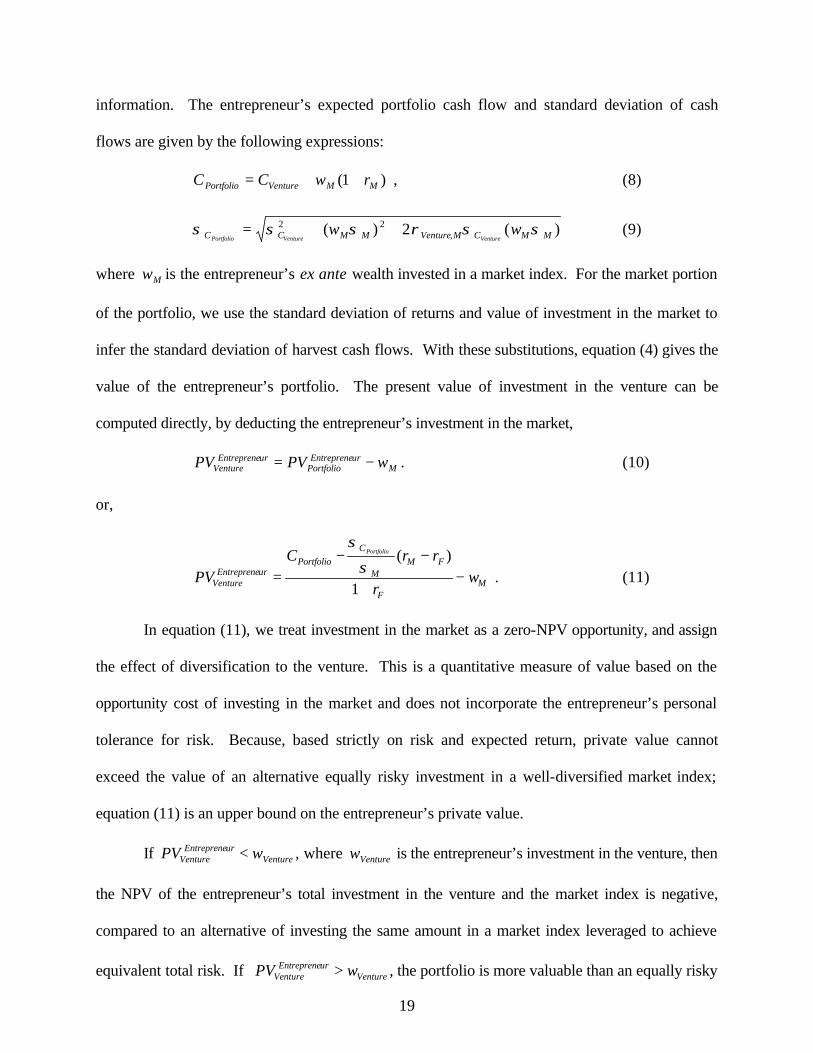
information. The entrepreneur’s expected portfolio cash flow and standard deviation of cash
flows are given by the following expressions:
)1( MMVenturePortfolio rwCC ++= , (8)
)(2)( ,22
MMCMVentureMMCC wwVentureVenturePortfolio
σσρσσσ ++= (9)
where Mw is the entrepreneur’s ex ante wealth invested in a market index. For the market portion
of the portfolio, we use the standard deviation of returns and value of investment in the market to
infer the standard deviation of harvest cash flows. With these substitutions, equation (4) gives the
value of the entrepreneur’s portfolio. The present value of investment in the venture can be
computed directly, by deducting the entrepreneur’s investment in the market,
MurEntreprene
PortfoliourEntreprene
Venture wPVPV −= . (10)
or,
MF
FMM
C
PortfoliourEntreprene
Venture wr
rrCPV
Portfolio
−+
−−=
1
)(σ
σ
. (11)
In equation (11), we treat investment in the market as a zero-NPV opportunity, and assign
the effect of diversification to the venture. This is a quantitative measure of value based on the
opportunity cost of investing in the market and does not incorporate the entrepreneur’s personal
tolerance for risk. Because, based strictly on risk and expected return, private value cannot
exceed the value of an alternative equally risky investment in a well-diversified market index;
equation (11) is an upper bound on the entrepreneur’s private value.
If VentureurEntreprene
Venture wPV < , where Venturew is the entrepreneur’s investment in the venture, then
the NPV of the entrepreneur’s total investment in the venture and the market index is negative,
compared to an alternative of investing the same amount in a market index leveraged to achieve
equivalent total risk. If VentureurEntreprene
Venture wPV > , the portfolio is more valuable than an equally risky
20
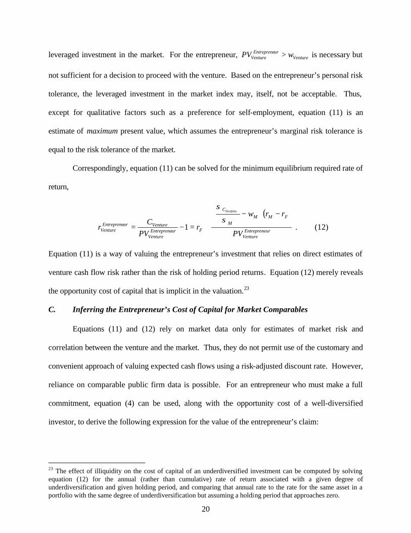
leveraged investment in the market. For the entrepreneur, VentureurEntreprene
Venture wPV > is necessary but
not sufficient for a decision to proceed with the venture. Based on the entrepreneur’s personal risk
tolerance, the leveraged investment in the market index may, itself, not be acceptable. Thus,
except for qualitative factors such as a preference for self-employment, equation (11) is an
estimate of maximum present value, which assumes the entrepreneur’s marginal risk tolerance is
equal to the risk tolerance of the market.
Correspondingly, equation (11) can be solved for the minimum equilibrium required rate of
return,
( )
urEntrepreneVenture
FMMM
C
FurEntrepreneVenture
VentureurEntrepreneVenture PV
rrw
rPV
Cr
Portfolio −
−
+=−=σ
σ
1 . (12)
Equation (11) is a way of valuing the entrepreneur’s investment that relies on direct estimates of
venture cash flow risk rather than the risk of holding period returns. Equation (12) merely reveals
the opportunity cost of capital that is implicit in the valuation.23
C. Inferring the Entrepreneur’s Cost of Capital for Market Comparables
Equations (11) and (12) rely on market data only for estimates of market risk and
correlation between the venture and the market. Thus, they do not permit use of the customary and
convenient approach of valuing expected cash flows using a risk-adjusted discount rate. However,
reliance on comparable public firm data is possible. For an entrepreneur who must make a full
commitment, equation (4) can be used, along with the opportunity cost of a well-diversified
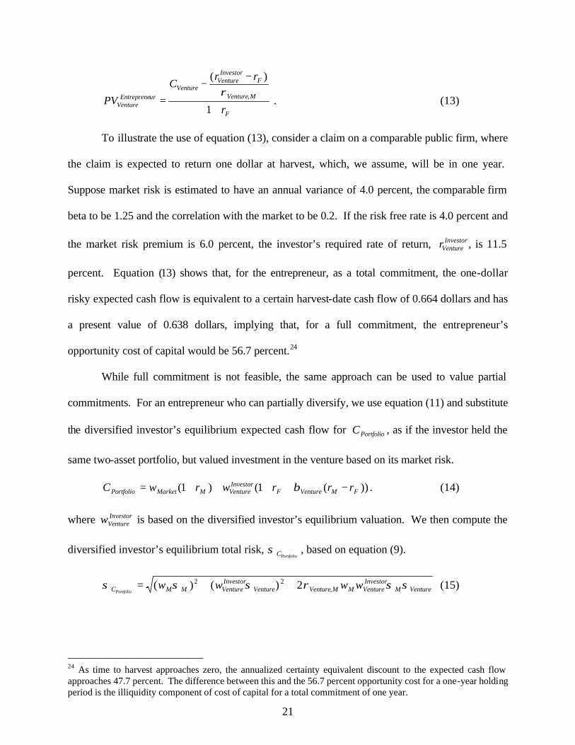
investor, to derive the following expression for the value of the entrepreneur’s claim:
23 The effect of illiquidity on the cost of capital of an underdiversified investment can be computed by solving equation (12) for the annual (rather than cumulative) rate of return associated with a given degree of underdiversification and given holding period, and comparing that annual rate to the rate for the same asset in a portfolio with the same degree of underdiversification but assuming a holding period that approaches zero.
21
F
MVenture
FInvestor
VentureVenture
urEntrepreneVenture r
rrC
PV+
−−
=1
)(
,ρ . (13)
To illustrate the use of equation (13), consider a claim on a comparable public firm, where
the claim is expected to return one dollar at harvest, which, we assume, will be in one year.
Suppose market risk is estimated to have an annual variance of 4.0 percent, the comparable firm
beta to be 1.25 and the correlation with the market to be 0.2. If the risk free rate is 4.0 percent and
the market risk premium is 6.0 percent, the investor’s required rate of return, InvestorVenturer , is 11.5
percent. Equation (13) shows that, for the entrepreneur, as a total commitment, the one-dollar
risky expected cash flow is equivalent to a certain harvest-date cash flow of 0.664 dollars and has
a present value of 0.638 dollars, implying that, for a full commitment, the entrepreneur’s
opportunity cost of capital would be 56.7 percent.24
While full commitment is not feasible, the same approach can be used to value partial
commitments. For an entrepreneur who can partially diversify, we use equation (11) and substitute
the diversified investor’s equilibrium expected cash flow for PortfolioC , as if the investor held the
same two-asset portfolio, but valued investment in the venture based on its market risk.
))(1()1( FMVentureFInvestor
VentureMMarketPortfolio rrrwrwC −++++= β . (14)
where InvestorVenturew is based on the diversified investor’s equilibrium valuation. We then compute the
diversified investor’s equilibrium total risk, PortfolioCσ , based on equation (9).
VentureMInvestorVentureMMVentureVenture
InvestorVentureMMC wwww
Portfolioσσρσσσ ,
22 2)()( ++= (15)
24 As time to harvest approaches zero, the annualized certainty equivalent discount to the expected cash flow approaches 47.7 percent. The difference between this and the 56.7 percent opportunity cost for a one-year holding period is the illiquidity component of cost of capital for a total commitment of one year.

22
Equations (14) and (15) represent expected portfolio cash flows and cash flow risk inferred from
public firm data. The estimates can be used in equation (10) to find the present value of the
entrepreneur’s investment in the venture, and in equation (12) to find equilibrium cost of capital.
Continuing the illustration, consider a hypothetical total investment of one dollar by an
investor who prices only systematic risk, where $0.60 is invested in the market portfolio and
$0.40 is invested in a public firm comparable to the venture (with beta risk of 1.25 and correlation
of 0.2, as above). Based on the previously stated assumptions, the investor’s expected cash return
in one year is $1.106, including $0.66 from investment in the market and $0.446 from investment in
the comparable firm. Using equation (15) and the assumption that the annualized standard
deviation of market returns is 20 percent, the annualized standard deviation of the two-asset
portfolio cash flows is 53.7 percent. Using this information in equation (11), the value of the
entrepreneur’s portfolio is $0.909, reflecting the effect of underdiversification. Thus, the value of
the claim on the venture, which pays $0.446 in expected cash flow at harvest, is $0.309, which, in
relation to the investment of $0.60 in the market, accounts for 34.0 percent of the entrepreneur’s
total wealth. From equation (12), the entrepreneur’s opportunity cost of investing in the venture is
44.5 percent. Thus, even with this degree of diversification, the entrepreneur’s opportunity cost is
much higher than that of a well-diversified investor. To assess an opportunity with risk
characteristics similar to the public firm, an entrepreneur who anticipated committing 34.0 percent
of total wealth to the venture, and placing the balance in the market could discount expected cash
flows at the 44.5 percent rate.
V. Empirical Evidence on New Venture Opportunity Cost of Capital
In this section we present evidence that can be used to estimate cost of capital for investors
and entrepreneurs. For a well-diversified investor, equation (1) requires an estimate of the beta of
the financial claim. For the entrepreneur, equations (11) through (15) require an estimate of the
23
risk of holding period returns for a well-diversified investor and an estimate of the correlation
with the market.
A. Data and Method
Because we are interested in early-stage firms and in how corporate maturity and financial
condition affect risk, we concentrate on newly public firms in technologically oriented industries.
Results are based on eight industries, as defined by Market Guide, that attract significant amounts
of venture capital investment: Biotechnology, Broadcast and Cable TV, Communication
Equipment, Communication Services, Computer Networks, Computer Services, Retail Catalog and
Mail Order (including Internet), and Software. Yahoo is our primary source of stock performance
data because the Yahoo data are maintained continuously and are current. We use financial data
from Compustat, supplemented with data from Market Guide.
The database includes all firms in the eight industries that went public between l995 and
late 2000. We define an observation as a calendar firm-year. Because risk attributes may change
with maturity, we use stock performance data from a single calendar year to estimate the risk
attributes of an observation. We match the most recent calendar year of stock price data to the
most recent fiscal year of financial data. Most observations have December 31 fiscal years. Thus,
stock performance for one calendar year is matched with financial data of the prior fiscal year.
We retain any observation for which at least 30 weeks of stock price data are available along with
financial reporting data for the corresponding fiscal year. Application of these screens results in a
total of 2,623 firm-year observations. Table 1 contains the breakdown by industry.
B. Bivariate Results
Tables 2 through 5 provide statistical information under headings of Calendar Year,
Industry, Firm Age, Financial Condition, and Employees. We measure firm age relative to the IPO
date. We also classify observations either as “from the year of the IPO” or “from years after the

24
IPO.” Financial condition classifications correspond to stages of firm development. If the firm
has no revenue during the year, it is an early-stage firm that may be engaged in research and
development before start-up of operations. If the firm has revenue but income is negative, it
generally is at a stage where it needs continuing external financing and may not have reached
sufficient scale to sustain operations from cash flow. Some of these observations are of troubled
firms, where previous years of positive income are followed by losses in the classification year.
If net income is positive, the firm may be sustainable with operating cash flows, though growth
still may require outside financing. We use number of employees as another measure of maturity
and size. The tables include quartile data to enable sensitivity analysis.
Beta: Table 2 contains beta estimates using the S&P500 Index as the market proxy.
Results are equilibrium equity betas for well-diversified investors.25 We use weekly returns,
rather than daily, as a convenient way to reduce bias due to nonsynchronous trading. We do not
compute asset betas. Most firms in our sample are early-stage and do not rely on debt financing.
The standard errors in Tables 2 through 5 can be used to make convenient inferences
regarding differences in mean values.26 Though, in these tables, we do not report significance
tests, interpretations of results are made in consideration of the statistical significance of
differences in means at the 5 percent level.
Although new ventures are risky, most of the risk is idiosyncratic. Table 2 shows an
overall average beta near 1.0 relative to the S&P500. The range across industries is from 0.75 to
1.24. We also estimate betas relative to the NASDAQ Composite Index and the PSE Technology
25 As implied by earlier discussion, due to lower valuations and higher equilibrium holding period returns and corresponding standard deviations, betas would be higher for underdiversified investors. 26 The standard error of the difference between any two means is somewhat less than the sum of the standard errors. Thus, dividing the difference by the sum of the two produces a negatively biased estimate of the t-value. On the other hand, because firms are included in the sample for several years (an average of 2.6 years), the observations are not independent. Lack of independence would positively bias the t-value. As we do not make strong statements of statistical significance between groups, we do not correct for either bias.

25
Index.27 The NASDAQ Index is a broad-based value-weighted index of the almost 4,000 stocks
listed on NASDAQ. Thus, it places more weight on small firms and high-tech firms. The PSE
Technology Index is the technology-oriented index with the longest history of returns. We use the
NASDAQ Composite and PSE Tech indexes to examine sensitivity of estimates to the market
capitalization and technology weightings of the market proxy. The average NASDAQ-based beta
in our sample is 0.72 and the average PSE Tech-based beta is 0.68.
For most years, the average betas in our sample are below 1.0 relative to the S&P500. In
1995 and 1996, when high-tech stocks represent a small fraction of market capitalization, average
betas are not significantly different from zero. Because market capitalization of high-tech stocks
had increased by 2000 and the market decline in 2000 was concentrated among technology and
growth firms, the high-tech attribute of the market index was stronger than in the other years. The
pattern is similar for annual average betas relative to the NASDAQ Composite and PSE Tech
indexes, though the beta estimates consistently are lower.
Irrespective of the index used, average betas increase significantly with age as a public
firm and with firm size. Betas are higher for firms with revenue but negative income than for those
with no revenue or with positive income. Only the latter difference is statistically significant at
conventional levels. The pattern with respect to financial condition suggests that, as firms mature,
they transition from risk that is highly idiosyncratic to risk more closely related to the market and
that market risk declines as profitably is achieved. Average betas are significantly different across
some industries. However, as most betas relative to the S&P500 are close to one, the economic
importance of the differences is limited. The Table 2 results imply that cost of capital for venture
capital investments is comparable to that of publicly traded stocks.
27 An appendix containing NASDAQ Composite and PSE Tech results is available on request.
26
Standard deviation of returns: As a basis for estimating opportunity cost for
underdiversified investors, we use the returns data to estimate of total risk and correlation with the
market. In Table 3, we report statistics for the annualized standard deviation of returns for well-
diversified investors.28 Because entrepreneurs cannot diversify fully, their equilibrium returns and
the corresponding standard deviations are higher.
The average annualized standard deviation of returns in our sample is 120 percent.
Differences between mean and median returns provide evidence of positive skewness, as median
returns consistently are lower than means. The means of the annualized standard deviations vary
significantly over years, but the variations are not systematic.
Total risk varies significantly across industries. Whereas our estimate of beta increases
with firm age and number of employees, total risk generally decreases modestly with increases in
age and number of employees. We also find a weak tendency for total risk to decline as financial
condition improves. Firm maturity should generally correspond to declining total risk and
possibly increasing market risk. Thus, the disparity between the entrepreneur’s opportunity cost
and that of a well-diversified investor is likely to be greatest for early-stage ventures.
Though Table 3 does not contain estimates of equilibrium standard deviations for
underdiversified entrepreneurs, the results imply that higher costs of capital should be used for
earlier stage ventures. Regardless of how the data are partitioned, the mean standard deviation
remains close to the 120 percent overall mean. The main exception is the high standard deviation
in the year of IPO. The implication is that, for estimating total risk, factors like stage of
development, financial condition, and firm size are of limited economic significance.
Total risk to market risk: In Table 4, we normalize total risk by the standard deviation of
returns on the S&P500 Index for the year. For the full sample, total risk is more than 5.6 times as
28 Standard deviations are annualized using weekly data, assuming time-series independence, and a 52-week year.

27
high as the risk of the S&P500 Index. The significant differences across industries, documented in
Table 3, persist when total risk is normalized by market risk. It is noteworthy, that the ratios
increase systematically over the six years of our study. The time-series is consistent with the trend
toward IPOs occurring at earlier stages of development. Correspondingly, the ratio tends to be
high in the year of the IPO, before the firm has achieved positive income, and where number of
employees is low. Nonetheless, most means are in the range of 4.0 to 6.5 times market risk.
The results suggest that one approach to estimating opportunity cost for either a well-
diversified or an underdiversified investor is to estimate total market risk, such as by using
implied volatilities from options on a market index, and then using Table 4 results to derive an
estimate of normalized total risk. This estimate, combined with an estimate of correlation with the
market, provides a simple alternative to estimating a venture’s total risk directly.29
Compared to the NASDAQ Composite, average total risk in our sample is 3.5 times as
high. Compared to the PSE Tech, average total risk is 3.04 times as high. Variations across
groupings are similar when total risk is compared to the NASDAQ Composite or PSE Tech index
over time, by financial maturity, or by industry.
Correlation with market returns: In Table 5, we report correlations between returns of
firm equity and the S&P500 Index. Correlations generally are low, as most new ventures are
narrowly focused, with cash flows that are not sensitive to market-wide cash flows. The average
correlation in our sample is 0.195. As implied by earlier results, the calendar-year means are
increasing from 1995 through 2000. The means in the first two years are not significantly different
from zero. Correlations with the S&P500 Index increase significantly with firm age, financial
condition, and number of employees. The low correlations point to the potential for value creation
by using financial contracts to shift risk to well-diversified investors.
29 For an underdiversified investor, this requires adjusting the total risk estimate as discussed in Section IV.

28
Correlations with the NASDAQ Composite and PSE Tech indexes are higher. Average
correlation with NASDAQ is 0.27, and average correlation with the PSE Tech is 0.23. Relative
differences vary by industry. Broadcast and Cable and Communications Services have S&P500
and NASDAQ correlations that are similar, whereas the other industries have higher NASDAQ
correlations. Industry correlations with the PSE Technology index are similar to those with
NASDAQ, except that the Computer Services correlation is similar to that with the S&P500.
C. Multivariate Results
In Table 6, we use regression analysis to examine the combined effects of industry, age,
and financial condition. The table summarizes results for three risk attributes: standard deviation
of returns, correlation with the S&P500 Index, and beta risk measured against the S&P500. Model
specifications intentionally are parsimonious. We estimate intercepts and age coefficients by
industry, and restrict revenue and income coefficients to be uniform across industries. While we
allow for the estimates to be different by calendar year, a forward-looking estimate normally
would be based on a representative average or a market volatility forecast. The model of the
standard deviation includes the market standard deviation as an explanatory variable. For
observations where a previous-year estimate is available, we include a lag term. For a firm’s first
observation, we code the lag as zero and assign a value of one to a “no lag” dummy variable.
Consistent with earlier discussion, total risk is positively related to market risk. A one-
percent increase in market risk corresponds to a 1.5 percent increase in total risk. Though
intercept differences usually are not significant, total risk is negatively related to firm maturity for
all industries.30 Positive revenue is not significantly related to total risk, but positive operating
income corresponds to a 3.3 percent reduction. The binary year variables evidence the variability
30 Except for Biotechnology, the intercept is the sum of the Biotechnology intercept and the industry-interacted intercept. Similarly, the age effect is the sum of the default age coefficient and the industry interaction with age.
29
of standard deviation estimates. In a forward-looking estimate, the average calendar year effect is
a –7.3 percent adjustment to the value derived from the other coefficients.
The correlation results indicate substantial variation across industries, though significance
levels are moderate. Operating income is again significant. The effects of firm maturity vary
significantly across industries. Correlations are significantly lower in other years than in the 2000,
which is the default year.
Beta risk also varies across industries and decreases with firm age. The relation with age
varies considerably across industries. Beta is lower for firms with operating income, though the
relation is only significant at the 10 percent level.
With regard to all three models, most of the explanatory power is associated with the
random year effects. The models also suggest that total risk decreases modestly with age and
financial condition, that correlation increases modestly with these factors, and that beta risk
increases with age but decreases with financial condition. For estimating opportunity cost, the
multivariate results provide little improvement over the bivariate results in Tables 2 through 5.
Consequently, reliance on the averages from this sample of early-stage public firms is likely to
work well across a broad range of industries, stages of development, and financial conditions.
To address the latter proposition more formally, Table 7 shows comparisons of group
averages with estimates derived from the regression models in Table 6. To develop the regression
estimates without conditioning on data that are not observable, we replace the calendar year
effects with the weighted average coefficient on the intercept and calendar year binary variables.
We also base the estimates on the historical average market standard deviation of returns of 20
percent, approximately the average in our sample. Table 7 shows that, for all data groupings, the
average predicted value is similar to the true group average. The last two columns compare the
standard deviations of differences between the actual values and the group averages with the

30
standard deviations of differences between the actual values and the predicted values based on the
regression models. The improvement in forecast accuracy from the regression approach is
reflected as a reduction in the standard deviation of the prediction errors. In all cases, the
improvement is slight.
D. Opportunity Cost of Capital
Table 8 contains estimates for all observations and by industry and stage of development of
opportunity cost for entrepreneur and well-diversified venture capital investors. The table is
based on an assumed annual equilibrium standard deviation of the market of 16.2 percent,
correlations from Table 5, and standard deviations for the groupings from Table 3.31 We base the
estimates on an assumed risk-free rate of 4.0 percent and market rate of 10.0 percent.
Cost of capital for well-diversified investors: Based on total risk of 102.1 percent and a
correlation of 0.195 with the market, the All-Observation beta, for example, is 0.99. Using our
market return assumptions, opportunity cost of a well-diversified investor is 11.4 percent. The
estimate is based on assumptions for the risk-free rate and market risk premium that both are
below historical averages but are consistent with the current environment.
In the context of a venture capital investment, or in cases where due diligence and other
investments of effort are not separately compensated, cost of capital must be grossed up to
compensate for investment of effort. Based on the normal 20 percent carried interest of venture
capital fund managers and a 2.5 percent annual management fee, the required gross return for the
All-Observations sample is about one-third higher, or 16.7 percent.
Cost of capital of the entrepreneur: In Table 8, we quantify the effect of
underdiversification on the entrepreneur’s opportunity cost. For an entrepreneur who must commit
total wealth, we use equations (11) and (12), but set Mw equal to zero. For full commitments,
31 The S&P500 annualized standard deviation is estimated based on the most recent 20 years of historical data.
31
opportunity cost is very high and varies considerably across industry and by financial maturity.
Whereas the investor’s cost of capital generally increases with firm maturity, the entrepreneur’s
opportunity cost generally decreases. Market risk rises, but total risk falls.
To infer realistic levels of entrepreneurial underdiversification, we considered a variety of
scenarios of the entrepreneur’s remaining work life, length of commitment to the venture, and
financial wealth that cannot be invested in the venture. Based on that analysis, it appears unlikely
that an entrepreneur could commit more than about 35 percent of total wealth to a venture. Even
that would involve an irrevocable commitment of human capital for several years.32 In the table,
we assume that an entrepreneur may commit 15 to 35 percent of total wealth. For example,
assuming the entrepreneur must invest 35 percent and can invest the balance in the market, we use
equations (11) and (12) to estimate the entrepreneur’s opportunity cost based on all observations.
The resulting estimate is 45.6 percent.
The difference between the entrepreneur’s cost of capital and the 16.7 percent gross-of-
fees opportunity cost of diversified investors suggests the potential to create value by contracting
to shift risk to the investor.33 With 25 percent of wealth in the venture, the entrepreneur’s cost of
capital declines to 40.0 percent. With 15 percent, it declines to 31.1 percent. Thus, reducing the
entrepreneur’s investment both transfers risk to the better-diversified investor and reduces the
entrepreneur’s cost of capital. Yet, even when the entrepreneur’s commitment represents a fairly
small fraction of total wealth and the balance is invested in the market, the difference between the
entrepreneur’s cost of capital and that of a venture capital investor is substantial.
32 To determine the human capital commitment, we estimate the present value of the entrepreneur’s income from continued employment until retirement at age 65. We then deduct the earnings from self-employment for the length of the assumed commitment and allow for the possibility that, if the venture were to fail or the entrepreneur were to leave the venture, the previous level of income could not be achieved. We assume the difference is a stream of cash that could have been invested in the market index. The present value is the entrepreneur’s human capital investment. 33 Heaton and Lucas (2001) use similar reasoning to explore the potential for value to be created through contracts that shift risk to well-diversified investors and reach similar conclusions.

32
As a short cut to estimating the entrepreneur’s cost of capital, we considered using the
standard deviation of holding period return estimates from Table 3 directly in Equation (5) and
then using Equations (3) and (6) to estimate the opportunity cost. Because estimates by this
approach are based on the equilibrium valuations of well-diversified investors they are negatively
biased estimates of the equilibrium underdiversification risk premium. The approach generally
understates the underdiversification risk premium estimates reflected in Table 8 by 5 to 20
percentage points. Even with only 15 percent of total wealth invested in the venture, the estimates
by this short-cut approach generally are 5 to 10 percentage points lower than equilibrium
estimates.
Sensitivity to assumptions: The estimates in Table 8 depend on specific assumptions
about the risk-free rate and market risk premium and include no differential return for investing in
small firms. For a well-diversified investor, the effects of different assumptions for any of these
factors are easily assessed using the CAPM. For an underdiversified investor the effects of
changing assumptions are less obvious. Based on the average of all observations, for example,
increasing the risk-free rate has a slightly less than additive effect of the cost of capital. Increasing
the risk-free rate by 1.0 percent increases the estimated cost of capital for an entrepreneur with 25
percent of wealth in the venture by 0.9 percent. For the same sample, cost of capital estimates are
highly sensitive to the assumed market risk premium. Increasing the market risk premium by 1.0
percent increases the estimated cost of capital for an entrepreneur with 25 percent of wealth in the
venture by 8.6 percent.
Except for adding an empirical estimate of small firm risk premium to the computed risk
premium (an approach that does not fit well within our framework), there is no obvious way to
estimate a small-firm risk premium for the entrepreneur’s underdiversified investment in the

33
venture.34 In the 18 years for which we have data on the PSE Tech Index, for example, the
annualized abnormal return of the index relative the S&P500 is 2.0 percent, similar to small firm
risk premium estimates reported in other sources. Assuming that the premium is not due to
informational asymmetry, as discussed above, and is not already captured in the illiquidity
component of the estimates, then arguably the cost of capital estimates of entrepreneurs and well-
diversified investors should be adjusted upward.
VI. Discussion
This paper develops a framework for evaluating investments in entrepreneurial ventures.
The framework is based on: applying the CAPM to determine opportunity cost of capital for well-
diversified investors, such as in the limited partners of venture capital funds; and recognizing that
entrepreneurs, as underdiversified investors, have opportunity costs of capital that can be
substantially higher than the rates that are appropriate for well-diversified investors.
We present evidence on the parameters that determine cost of capital for entrepreneurs and
well-diversified investors. The evidence, based on data for newly-public firms in eight high-tech
industries, indicates that total risk averages 5 times as high as market risk, correlations with
market returns are around 0.2, and equity betas are comparable to the overall market. While the
total risk of early-stage firms decreases with various indicia of maturity, market risk increases.
Our findings complement results of recent studies of hurdle rates for risk-averse
entrepreneurs. Using either a hurdle rate or opportunity cost as a decision criterion, returns for
underdiversified investments in new ventures would need to be substantially higher than returns for
investing in a diversified portfolio. Our evidence adds to these earlier findings, and is the only
study based on empirical data for recently public high-tech firms with limited track records.
34 Replacing a well-diversified market index with a small firm or technology stock index that is less well diversified is equivalent to constraining the entrepreneur to hold an inefficient proxy for the market. Imposing such a constraint incorrectly lowers the estimate of the entrepreneur’s cost of capital for investing in the venture.
34
The findings indicate that the entrepreneur’s cost of capital declines rapidly as the
fraction of wealth that must be invested in the venture declines. However, even with modest
underdiversification, the entrepreneur’s cost of capital is substantially higher than that of a well-
diversified investor. For reasonable levels of underdiversification and a one-year holding period,
underdiversification risk premia generally are 10 to 40 percent above the cost of capital of a well-
diversified investor. Even with 15 percent of wealth in the venture, underdiversification risk
premia are in the 10 to 30 percent range.
Depending on the industry and maturity of the venture and the fraction of the entrepreneur’s
financial and human capital that is committed to the venture, we estimate that the entrepreneur’s
cost of capital is two to four times as high as the cost of capital for a well-diversified investor.
Similarly, the entrepreneur’s cost is 1.5 to three times as high as our estimate of the gross-of-fee-
and-carried-interest required rate of return of venture capital funds.
The difference in cost of capital between underdiversified and well-diversified investors
is an important departure from the “Law of One Price.” Because the entrepreneur’s cost of capital
depends on total risk, opportunities exist for designing value-maximizing strategies for undertaking
new ventures. Strategies that reduce the total investment, such as by shortening the time to
abandonment or reducing scale or scope, can create value by reducing the entrepreneur’s
commitment, and hence lower the cost of capital. Holding total investment constant, contracts
between entrepreneurs and investors can enhance the value of an opportunity, and can turn
unacceptable ventures into attractive ones. In particular, contracts that shift risk to investors, such
as by increasing cash compensation to the entrepreneur or reducing the preferential treatment of
investors, can reduce the venture’s weighted average cost of capital.
Of course, differences in perception between the entrepreneur and the investor about the
likelihood of success, as well as adverse selection and moral hazard, all may favor contract

35
provisions that shift risk to the entrepreneur. Hence, the choices of new venture strategy and
allocations of risk reflect a set of trade-offs that includes the cost of capital differential between
the entrepreneur and the investor. More generally, our evidence points to the potentially large
economic cost of illiquid employee stock and option ownership positions and to the potential for
value to be created through going-public transactions.

References
Amihud, Yakov, and Haim Mendelson, 1986, Asset pricing and the bid ask spread, Journal of
Financial Economics 17, 223-249.
Benartzi, Shlomo, 2001, Excessive extrapolation and the allocation of 401 (k) accounts to
company stock, The Journal of Finance 56, 1747-1764.
Bernardo, Antonio, and Ivo Welch, 2001, On the evolution of overconfidence of entrepreneurs,
Journal of Economics and Management Strategy 10, 301-330.
Brennan, Michael J., and Walter N. Torous, 1999, Individual decision-making and investor
welfare, Economics Notes.
Bygrave, William D., and Jeffrey A. Timmons, 1992, Venture Capital at the Crossroads
(Harvard Business School Press, Boston).
Cochrane, John, 2001, The risk and return of venture capital, National Bureau of Economic
Research working paper no. 8066.
Cooper, Arnold C., Carolyn Y. Woo, and William C. Dunkelberg, 1988, Entrepreneurs’ perceived
chances of success, Journal of Business Venturing 3, 97-108.
Fama, Eugene, and Kenneth French, 1995, Size and book-to-market factors in earnings and returns,
The Journal of Finance 50, 131-155.
Garvey, Gerald T., 2001, What is an acceptable rate of return for an undiversified investor?
Claremont Graduate University working paper.
Gompers, Paul, and Josh Lerner, Winter 1997, Risk and reward in private equity investments: The
challenge of performance assessment,” Journal of Private Equity, 5-12.
Gompers, Paul, and Josh Lerner, 1999, An analysis of compensation in the U. S. venture capital
partnership,” Journal of Financial Economics 51, 3-44.
Hall, Brian J. and Kevin J. Murphy. 2002, Stock options for undiversified executives,” Journal of
Accounting and Economics 33, 3-42.
Hamilton, Barton, 2000, Does entrepreneurship pay? An empirical analysis of the returns to self-
employment, Journal of Political Economy 108, 604-631.
Heaton, John and Deborah Lucas, 2000, Portfolio choice and asset prices: The importance of
entrepreneurial risk, The Journal of Finance 55, 1163-1198.
Heaton, John and Deborah Lucas, 2001, “Capital structure, hurdle rates, and portfolio choice—
Interactions in an entrepreneurial firm, University of Chicago working paper.
Ibbotson, Roger G., and Gary P. Brinson, 1987, Investment Markets (McGraw Hill, New York).

2
Jagannathan, Ravi, and Zhenyu Wang, The conditional CAPM and the cross-section of expected
returns, The Journal of Finance 51, 3-53.
Jones, Charles M., and Matthew Rhodes-Kropf, 2002, The price of diversifiable risk in venture
capital and private equity, Columbia University working paper.
Longstaff, Francis, 1995, How much can marketability affect security values? The Journal of
Finance 50, 1767-1774.
Martin, John D., and William Petty, 1983, An analysis of the performance of publicly traded
venture capital companies, Journal of Financial and Quantitative Analysis 18, 401-410.
Mayers, David, 1976, Nonmarketable assets, market segmentation, and the level of asset prices,
Journal of Financial and Quantitative Analysis, 1-12.
Meulbroek, Lisa, 2002, Company stock in pension plans: How costly is it? Harvard Business
School working paper.
Moskowitz, Tobias, J., and Annette Vissing-Jørgensen, 2002, The returns to entrepreneurial
investment: A private equity premium puzzle? American Economic Review 92, 745-778.
Sahlman, William A., 1990, The structure and governance of venture-capital organizations,
Journal of Financial Economics 27, 473-524.
Van Osnabrugge, Mark, and Robert J. Robinson, 2000, Angel Investing (Jossey-Bass, San
Francisco).
Venture Economics, 1997, Investment Benchmarks: Venture Capital.
Venture Economics, Press releases at www.ventureconomics.com.
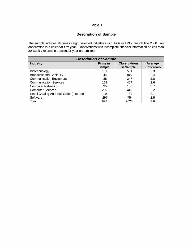
Table 1
Description of Sample
The sample includes all firms in eight selected industries with IPOs in 1995 through late 2000. An observation is a calendar firm-year. Observations with incomplete financial information or less than 30 weekly returns in a calendar year are omitted.
Description of Sample Industry Firms in
Sample Observations
in Sample Average
Firm-Years Biotechnology 151 501 3.3 Broadcast and Cable TV 44 105 2.4 Communication Equipment 88 247 2.8 Communication Services 158 407 2.6 Computer Network 35 130 3.7 Computer Services 200 440 2.2 Retail Catalog And Mail Order (Internet) 19 39 2.1 Software 297 754 2.5 Total 992 2623 2.6
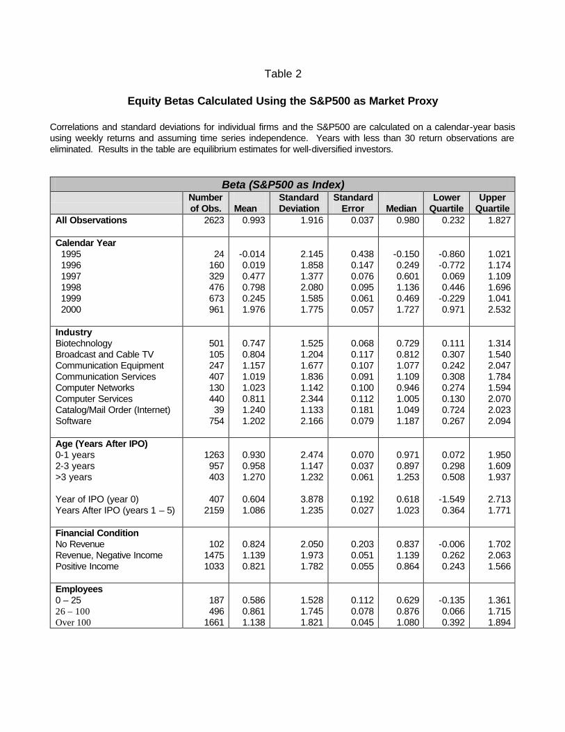
Table 2
Equity Betas Calculated Using the S&P500 as Market Proxy
Correlations and standard deviations for individual firms and the S&P500 are calculated on a calendar-year basis using weekly returns and assuming time series independence. Years with less than 30 return observations are eliminated. Results in the table are equilibrium estimates for well-diversified investors.
Beta (S&P500 as Index) Number
of Obs.
Mean Standard Deviation
Standard Error
Median
Lower Quartile
Upper Quartile
All Observations 2623 0.993 1.916 0.037 0.980 0.232 1.827 Calendar Year 1995 24 -0.014 2.145 0.438 -0.150 -0.860 1.021 1996 160 0.019 1.858 0.147 0.249 -0.772 1.174 1997 329 0.477 1.377 0.076 0.601 0.069 1.109 1998 476 0.798 2.080 0.095 1.136 0.446 1.696 1999 673 0.245 1.585 0.061 0.469 -0.229 1.041 2000 961 1.976 1.775 0.057 1.727 0.971 2.532 Industry Biotechnology 501 0.747 1.525 0.068 0.729 0.111 1.314 Broadcast and Cable TV 105 0.804 1.204 0.117 0.812 0.307 1.540 Communication Equipment 247 1.157 1.677 0.107 1.077 0.242 2.047 Communication Services 407 1.019 1.836 0.091 1.109 0.308 1.784 Computer Networks 130 1.023 1.142 0.100 0.946 0.274 1.594 Computer Services 440 0.811 2.344 0.112 1.005 0.130 2.070 Catalog/Mail Order (Internet) 39 1.240 1.133 0.181 1.049 0.724 2.023 Software 754 1.202 2.166 0.079 1.187 0.267 2.094 Age (Years After IPO) 0-1 years 1263 0.930 2.474 0.070 0.971 0.072 1.950 2-3 years 957 0.958 1.147 0.037 0.897 0.298 1.609 >3 years 403 1.270 1.232 0.061 1.253 0.508 1.937 Year of IPO (year 0) 407 0.604 3.878 0.192 0.618 -1.549 2.713 Years After IPO (years 1 – 5) 2159 1.086 1.235 0.027 1.023 0.364 1.771 Financial Condition No Revenue 102 0.824 2.050 0.203 0.837 -0.006 1.702 Revenue, Negative Income 1475 1.139 1.973 0.051 1.139 0.262 2.063 Positive Income 1033 0.821 1.782 0.055 0.864 0.243 1.566 Employees 0 – 25 187 0.586 1.528 0.112 0.629 -0.135 1.361 26 – 100 496 0.861 1.745 0.078 0.876 0.066 1.715 Over 100 1661 1.138 1.821 0.045 1.080 0.392 1.894
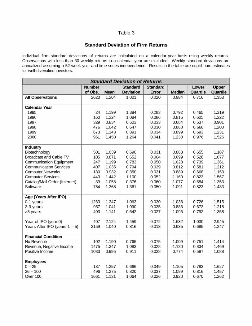
Table 3
Standard Deviation of Firm Returns
Individual firm standard deviations of returns are calculated on a calendar-year basis using weekly returns. Observations with less than 30 weekly returns in a calendar year are excluded. Weekly standard deviations are annualized assuming a 52-week year and time series independence. Results in the table are equilibrium estimates for well-diversified investors.
Standard Deviation of Returns Number
of Obs.
Mean Standard Deviation
Standard Error
Median
Lower Quartile
Upper Quartile
All Observations 2623 1.204 1.021 0.020 0.984 0.716 1.353 Calendar Year 1995 24 1.199 1.384 0.283 0.792 0.465 1.319 1996 160 1.224 1.084 0.086 0.815 0.605 1.222 1997 329 0.834 0.603 0.033 0.684 0.537 0.901 1998 476 1.042 0.647 0.030 0.868 0.666 1.200 1999 673 1.143 0.891 0.034 0.899 0.693 1.231 2000 961 1.450 1.264 0.041 1.238 0.976 1.526 Industry Biotechnology 501 1.039 0.696 0.031 0.868 0.655 1.187 Broadcast and Cable TV 105 0.871 0.652 0.064 0.699 0.528 1.077 Communication Equipment 247 1.199 0.783 0.050 1.028 0.739 1.361 Communication Services 407 1.035 0.794 0.039 0.812 0.581 1.212 Computer Networks 130 0.932 0.350 0.031 0.889 0.668 1.153 Computer Services 440 1.442 1.100 0.052 1.160 0.823 1.567 Catalog/Mail Order (Internet) 39 1.058 0.376 0.060 1.077 0.684 1.353 Software 754 1.368 1.361 0.050 1.091 0.823 1.433 Age (Years After IPO) 0-1 years 1263 1.347 1.063 0.030 1.038 0.726 1.515 2-3 years 957 1.041 1.090 0.035 0.886 0.673 1.218 >3 years 403 1.141 0.542 0.027 1.096 0.792 1.358 Year of IPO (year 0) 407 2.124 1.459 0.072 1.632 1.030 2.945 Years After IPO (years 1 – 5) 2159 1.040 0.816 0.018 0.935 0.685 1.247 Financial Condition No Revenue 102 1.190 0.765 0.075 1.009 0.751 1.414 Revenue, Negative Income 1475 1.347 1.083 0.028 1.130 0.834 1.469 Positive Income 1033 0.995 0.911 0.028 0.774 0.587 1.088 Employees 0 – 25 187 1.257 0.666 0.049 1.105 0.783 1.627 26 – 100 496 1.275 0.820 0.037 1.099 0.816 1.457 Over 100 1661 1.131 1.064 0.026 0.920 0.670 1.262
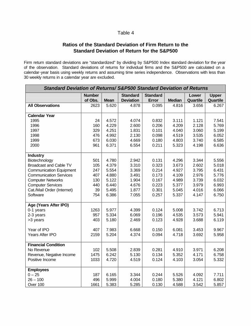
Table 4
Ratios of the Standard Deviation of Firm Return to the Standard Deviation of Return for the S&P500
Firm return standard deviations are “standardized” by dividing by S&P500 Index standard deviation for the year of the observation. Standard deviations of returns for individual firms and the S&P500 are calculated on a calendar-year basis using weekly returns and assuming time series independence. Observations with less than 30 weekly returns in a calendar year are excluded.
Standard Deviation of Returns/ S&P500 Standard Deviation of Returns Number
of Obs.
Mean Standard Deviation
Standard Error
Median
Lower Quartile
Upper Quartile
All Observations 2623 5.620 4.878 0.095 4.816 3.656 6.267 Calendar Year 1995 24 4.572 4.074 0.832 3.111 1.121 7.541 1996 160 4.229 2.600 0.206 4.209 2.128 5.769 1997 329 4.251 1.831 0.101 4.040 3.060 5.199 1998 476 4.992 2.130 0.098 4.519 3.535 6.052 1999 673 6.030 4.669 0.180 4.803 3.740 6.585 2000 961 6.371 6.554 0.211 5.323 4.198 6.636 Industry Biotechnology 501 4.780 2.942 0.131 4.296 3.344 5.556 Broadcast and Cable TV 105 4.379 3.310 0.323 3.673 2.602 5.018 Communication Equipment 247 5.554 3.369 0.214 4.927 3.795 6.431 Communication Services 407 4.880 3.491 0.173 4.109 2.976 5.776 Computer Networks 130 5.122 1.904 0.167 4.989 3.739 6.032 Computer Services 440 6.440 4.676 0.223 5.377 3.979 6.993 Cat./Mail Order (Internet) 39 5.495 1.877 0.301 5.045 4.016 6.066 Software 754 6.386 7.055 0.257 5.337 4.147 6.750 Age (Years After IPO) 0-1 years 1263 5.977 4.399 0.124 5.008 3.742 6.713 2-3 years 957 5.334 6.069 0.196 4.535 3.573 5.941 >3 years 403 5.180 2.469 0.123 4.928 3.688 6.119 Year of IPO 407 7.983 6.668 0.150 6.081 3.453 9.967 Years After IPO 2159 5.204 4.374 0.094 4.718 3.692 5.958 Financial Condition No Revenue 102 5.508 2.839 0.281 4.910 3.971 6.208 Revenue, Negative Income 1475 6.242 5.130 0.134 5.352 4.171 6.758 Positive Income 1033 4.720 4.519 0.124 4.103 3.054 5.332 Employees 0 – 25 187 6.165 3.344 0.244 5.526 4.092 7.711 26 – 100 496 5.999 4.004 0.180 5.380 4.121 6.802 Over 100 1661 5.383 5.285 0.130 4.588 3.542 5.857
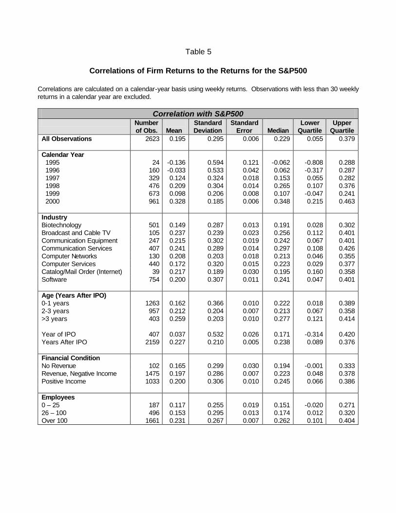
Table 5
Correlations of Firm Returns to the Returns for the S&P500
Correlations are calculated on a calendar-year basis using weekly returns. Observations with less than 30 weekly returns in a calendar year are excluded.
Correlation with S&P500 Number
of Obs.
Mean Standard Deviation
Standard Error
Median
Lower Quartile
Upper Quartile
All Observations 2623 0.195 0.295 0.006 0.229 0.055 0.379 Calendar Year 1995 24 -0.136 0.594 0.121 -0.062 -0.808 0.288 1996 160 -0.033 0.533 0.042 0.062 -0.317 0.287 1997 329 0.124 0.324 0.018 0.153 0.055 0.282 1998 476 0.209 0.304 0.014 0.265 0.107 0.376 1999 673 0.098 0.206 0.008 0.107 -0.047 0.241 2000 961 0.328 0.185 0.006 0.348 0.215 0.463 Industry Biotechnology 501 0.149 0.287 0.013 0.191 0.028 0.302 Broadcast and Cable TV 105 0.237 0.239 0.023 0.256 0.112 0.401 Communication Equipment 247 0.215 0.302 0.019 0.242 0.067 0.401 Communication Services 407 0.241 0.289 0.014 0.297 0.108 0.426 Computer Networks 130 0.208 0.203 0.018 0.213 0.046 0.355 Computer Services 440 0.172 0.320 0.015 0.223 0.029 0.377 Catalog/Mail Order (Internet) 39 0.217 0.189 0.030 0.195 0.160 0.358 Software 754 0.200 0.307 0.011 0.241 0.047 0.401 Age (Years After IPO) 0-1 years 1263 0.162 0.366 0.010 0.222 0.018 0.389 2-3 years 957 0.212 0.204 0.007 0.213 0.067 0.358 >3 years 403 0.259 0.203 0.010 0.277 0.121 0.414 Year of IPO 407 0.037 0.532 0.026 0.171 -0.314 0.420 Years After IPO 2159 0.227 0.210 0.005 0.238 0.089 0.376 Financial Condition No Revenue 102 0.165 0.299 0.030 0.194 -0.001 0.333 Revenue, Negative Income 1475 0.197 0.286 0.007 0.223 0.048 0.378 Positive Income 1033 0.200 0.306 0.010 0.245 0.066 0.386 Employees 0 – 25 187 0.117 0.255 0.019 0.151 -0.020 0.271 26 – 100 496 0.153 0.295 0.013 0.174 0.012 0.320 Over 100 1661 0.231 0.267 0.007 0.262 0.101 0.404

Table 6
Risk Attribute Regression Results
Regressions include both industry dummies for the intercept term and industry dummies interacted with the Age variable for the slope of the Age variable. Biotechnology is the baseline industry for the regressions. The baseline year is 2000. The S&P500 standard deviation is estimated from weekly returns for the contemporaneous year. Firm Age is measured as years since the IPO. Revenue equals one if the observation is associated with positive revenues and zero otherwise. Operating Income equals one if operating income is positive and zero otherwise. For the first year in a series, a binary (“No Lag”) variable is included and the lagged dependent variable value is zero.
Standard Deviation
of Returns Correlation with S&P500 Index
Beta Based on S&P500 Index
Variable Coefficient t Value Coefficient t Value Coefficient t Value Intercept (Biotech Industry, year 2000) 0.156 5.25** 0.391 6.55** 2.609 6.74** Broadcast and Cable TV Dummy 0.011 0.25 -0.105 -1.18 -0.999 -1.73 Communication Equipment Dummy 0.028 0.91 -0.095 -1.46 -0.564 -1.33 Communication Services Dummy 0.034 1.17 -0.092 -1.50 -0.646 -1.62 Computer Network Dummy 0.018 0.38 0.140 1.44 0.969 1.53 Computer Services Dummy 0.195 6.28** -0.283 -4.35** -1.772 -4.18** Retail Catalog Dummy -0.029 -0.37 0.081 0.50 0.393 0.37 Software Dummy 0.059 2.26* -0.142 -2.59** -0.386 -1.09 S&P500 Std. Deviation 1.466 9.51** Firm Age (Biotech Industry) -0.028 -1.66 -0.078 -2.20* -0.599 -2.61** Firm Age * Bdcst and Cble TV Dummy -0.023 -0.73 0.134 2.01* 0.736 1.70 Firm Age * Comm Equip Dummy -0.001 -0.05 0.116 2.42* 0.717 2.30* Firm Age * Comm Services Dummy -0.026 -1.20 0.130 2.87** 0.647 2.19* Firm Age * CompNet Dummy -0.004 -0.13 -0.047 -0.68 -0.400 -0.90 Firm Age * CompServ Dummy -0.128 -5.49** 0.220 4.49** 1.291 4.04** Firm Age * RetailCat Dummy 0.024 0.40 -0.040 -0.32 -0.173 -0.21 Firm Age * Software Dummy -0.014 -0.73 0.130 3.27** 0.535 2.06* 1995 Dummy -0.152 -5.27** -0.431 -7.38** -2.078 -5.47** 1996 Dummy -0.107 -8.71** -0.357 -14.45** -2.094 -12.99** 1997 Dummy -0.098 -11.39** -0.216 -11.85** -1.616 -13.59** 1998 Dummy -0.050 -6.74** -0.130 -8.35** -1.221 -12.06** 1999 Dummy -0.031 -4.74** -0.244 -17.69** -1.758 -19.56** Revenue (binary) -0.006 -0.43 -0.022 -0.78 -0.044 -0.24 Operating Income (binary) -0.029 -5.36** 0.018 1.59 -0.134 -1.81 No Lag Dummy 0.056 7.10** 0.011 0.63 0.152 1.43 Lagged Dependent Variable 0.139 5.23** 0.182 5.22** 0.129 3.07** Adj. r2 0.204 0.187 0.179
** Significant at the .01 level. * Significant at the .05 level.

Table 7
Comparisons of Regression Model Estimates with Group Means
The table shows standard deviations of (Actual – Mean) and (Actual – Predicted) and indicates that group means are almost as accurate as regression models at estimating the actual values of risk measures. Estimates are based on a market standard deviation of 0.20 and the weighted average of coefficients on calendar-year binary variables.
Mean of
Observations Mean of
Predictions Standard Deviation:
Actual - Mean Standard Deviation: Actual - Predicted
Standard Deviation All Observations 1.204 1.174 1.004 0.956 Broadcast & Cable TV 0.871 0.870 0.652 0.608 Biotechnology 1.039 1.031 0.696 0.683 Communication Equipment 1.199 1.186 0.783 0.731 Communication Services 1.035 1.020 0.794 0.746 Computer Networks 0.932 1.055 0.350 0.403 Computer Services 1.442 1.340 1.100 0.973 Retail Catalog/Mail Order 1.058 1.051 0.376 0.340 Software 1.368 1.323 1.361 1.326 Year of IPO 2.124 1.590 1.419 1.387 Years After IPO 1.040 1.086 0.810 0.819 No Revenue 1.190 1.216 0.756 0.689 Revenue, Negative Income 1.347 1.275 1.064 1.035 Positive Income 0.995 1.025 0.895 0.853
Correlation Coefficient All Observations 0.195 0.195 0.294 0.290 Broadcast & Cable TV 0.237 0.237 0.239 0.229 Biotechnology 0.149 0.161 0.287 0.290 Communication Equipment 0.215 0.221 0.302 0.299 Communication Services 0.241 0.246 0.289 0.277 Computer Networks 0.208 0.234 0.203 0.210 Computer Services 0.172 0.156 0.320 0.309 Retail Catalog/Mail Order 0.217 0.201 0.189 0.188 Software 0.200 0.191 0.307 0.307 Year of IPO 0.037 0.157 0.532 0.529 Years After IPO 0.227 0.203 0.207 0.210 No Revenue 0.165 0.187 0.311 0.287 Revenue, Negative Income 0.197 0.179 0.284 0.286 Positive Income 0.200 0.219 0.305 0.295
Betas All Observations 0.993 0.999 1.907 1.903 Broadcast & Cable TV 0.804 0.784 1.204 1.178 Biotechnology 0.747 0.849 1.525 1.561 Communication Equipment 1.157 1.190 1.677 1.673 Communication Services 1.019 1.045 1.836 1.842 Computer Networks 1.023 1.212 1.142 1.208 Computer Services 0.811 0.715 2.344 2.271 Retail Catalog/Mail Order 1.240 1.072 1.133 1.142 Software 1.202 1.165 2.166 2.174 Year of IPO 0.604 1.026 3.864 3.843 Years After IPO 1.086 0.991 1.224 1.235 No Revenue 0.824 0.978 2.170 1.998

Revenue, Negative Income 1.139 1.026 1.959 1.980 Positive Income 0.821 0.963 1.775 1.768
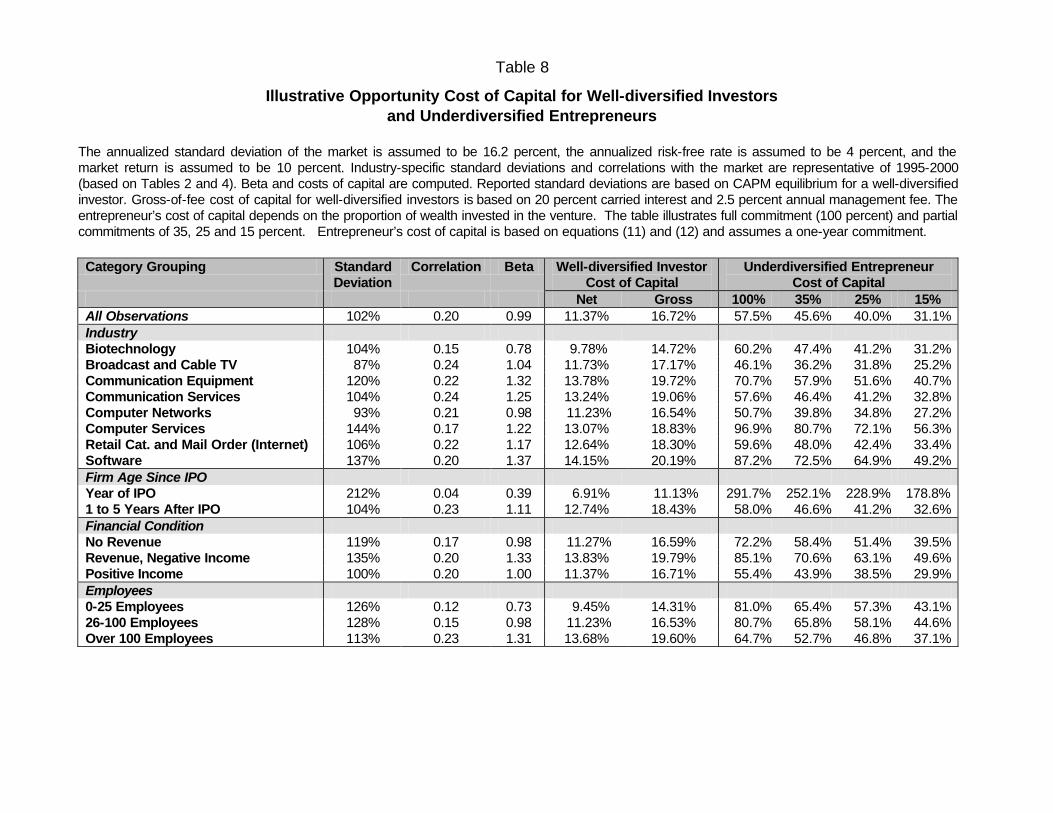
Table 8
Illustrative Opportunity Cost of Capital for Well-diversified Investors and Underdiversified Entrepreneurs
The annualized standard deviation of the market is assumed to be 16.2 percent, the annualized risk-free rate is assumed to be 4 percent, and the market return is assumed to be 10 percent. Industry-specific standard deviations and correlations with the market are representative of 1995-2000 (based on Tables 2 and 4). Beta and costs of capital are computed. Reported standard deviations are based on CAPM equilibrium for a well-diversified investor. Gross-of-fee cost of capital for well-diversified investors is based on 20 percent carried interest and 2.5 percent annual management fee. The entrepreneur’s cost of capital depends on the proportion of wealth invested in the venture. The table illustrates full commitment (100 percent) and partial commitments of 35, 25 and 15 percent. Entrepreneur’s cost of capital is based on equations (11) and (12) and assumes a one-year commitment.
Category Grouping Standard
Deviation Correlation Beta Well-diversified Investor
Cost of Capital Underdiversified Entrepreneur
Cost of Capital Net Gross 100% 35% 25% 15%
All Observations 102% 0.20 0.99 11.37% 16.72% 57.5% 45.6% 40.0% 31.1% Industry Biotechnology 104% 0.15 0.78 9.78% 14.72% 60.2% 47.4% 41.2% 31.2% Broadcast and Cable TV 87% 0.24 1.04 11.73% 17.17% 46.1% 36.2% 31.8% 25.2% Communication Equipment 120% 0.22 1.32 13.78% 19.72% 70.7% 57.9% 51.6% 40.7% Communication Services 104% 0.24 1.25 13.24% 19.06% 57.6% 46.4% 41.2% 32.8% Computer Networks 93% 0.21 0.98 11.23% 16.54% 50.7% 39.8% 34.8% 27.2% Computer Services 144% 0.17 1.22 13.07% 18.83% 96.9% 80.7% 72.1% 56.3% Retail Cat. and Mail Order (Internet) 106% 0.22 1.17 12.64% 18.30% 59.6% 48.0% 42.4% 33.4% Software 137% 0.20 1.37 14.15% 20.19% 87.2% 72.5% 64.9% 49.2% Firm Age Since IPO Year of IPO 212% 0.04 0.39 6.91% 11.13% 291.7% 252.1% 228.9% 178.8% 1 to 5 Years After IPO 104% 0.23 1.11 12.74% 18.43% 58.0% 46.6% 41.2% 32.6% Financial Condition No Revenue 119% 0.17 0.98 11.27% 16.59% 72.2% 58.4% 51.4% 39.5% Revenue, Negative Income 135% 0.20 1.33 13.83% 19.79% 85.1% 70.6% 63.1% 49.6% Positive Income 100% 0.20 1.00 11.37% 16.71% 55.4% 43.9% 38.5% 29.9% Employees 0-25 Employees 126% 0.12 0.73 9.45% 14.31% 81.0% 65.4% 57.3% 43.1% 26-100 Employees 128% 0.15 0.98 11.23% 16.53% 80.7% 65.8% 58.1% 44.6% Over 100 Employees 113% 0.23 1.31 13.68% 19.60% 64.7% 52.7% 46.8% 37.1%

Appendix (Available On Request)
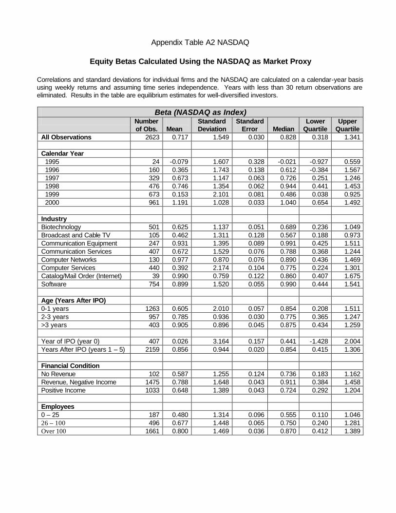
Appendix Table A2 NASDAQ
Equity Betas Calculated Using the NASDAQ as Market Proxy
Correlations and standard deviations for individual firms and the NASDAQ are calculated on a calendar-year basis using weekly returns and assuming time series independence. Years with less than 30 return observations are eliminated. Results in the table are equilibrium estimates for well-diversified investors.
Beta (NASDAQ as Index) Number
of Obs.
Mean Standard Deviation
Standard Error
Median
Lower Quartile
Upper Quartile
All Observations 2623 0.717 1.549 0.030 0.828 0.318 1.341 Calendar Year 1995 24 -0.079 1.607 0.328 -0.021 -0.927 0.559 1996 160 0.365 1.743 0.138 0.612 -0.384 1.567 1997 329 0.673 1.147 0.063 0.726 0.251 1.246 1998 476 0.746 1.354 0.062 0.944 0.441 1.453 1999 673 0.153 2.101 0.081 0.486 0.038 0.925 2000 961 1.191 1.028 0.033 1.040 0.654 1.492 Industry Biotechnology 501 0.625 1.137 0.051 0.689 0.236 1.049 Broadcast and Cable TV 105 0.462 1.311 0.128 0.567 0.188 0.973 Communication Equipment 247 0.931 1.395 0.089 0.991 0.425 1.511 Communication Services 407 0.672 1.529 0.076 0.788 0.368 1.244 Computer Networks 130 0.977 0.870 0.076 0.890 0.436 1.469 Computer Services 440 0.392 2.174 0.104 0.775 0.224 1.301 Catalog/Mail Order (Internet) 39 0.990 0.759 0.122 0.860 0.407 1.675 Software 754 0.899 1.520 0.055 0.990 0.444 1.541 Age (Years After IPO) 0-1 years 1263 0.605 2.010 0.057 0.854 0.208 1.511 2-3 years 957 0.785 0.936 0.030 0.775 0.365 1.247 >3 years 403 0.905 0.896 0.045 0.875 0.434 1.259 Year of IPO (year 0) 407 0.026 3.164 0.157 0.441 -1.428 2.004 Years After IPO (years 1 – 5) 2159 0.856 0.944 0.020 0.854 0.415 1.306 Financial Condition No Revenue 102 0.587 1.255 0.124 0.736 0.183 1.162 Revenue, Negative Income 1475 0.788 1.648 0.043 0.911 0.384 1.458 Positive Income 1033 0.648 1.389 0.043 0.724 0.292 1.204 Employees 0 – 25 187 0.480 1.314 0.096 0.555 0.110 1.046 26 – 100 496 0.677 1.448 0.065 0.750 0.240 1.281 Over 100 1661 0.800 1.469 0.036 0.870 0.412 1.389

Appendix Table A4 NASDAQ
Ratios of the Standard Deviation of Firm Return to the Standard Deviation of Return for the NASDAQ
Firm return standard deviations are “standardized” by dividing by NASDAQ Index standard deviation for the year of the observation. Standard deviations of returns for individual firms and the NASDAQ are calculated on a calendar-year basis using weekly returns and assuming time series independence. Observations with less than 30 weekly returns in a calendar year are excluded.
Standard Deviation of Returns/ NASDAQ Standard Deviation of Returns Number
of Obs.
Mean Standard Deviation
Standard Error
Median
Lower Quartile
Upper Quartile
All Observations 2623 3.464 2.599 0.051 2.968 2.177 4.146 Calendar Year 1995 24 2.574 2.020 0.412 2.084 0.889 4.019 1996 160 3.639 2.291 0.181 3.596 1.861 4.977 1997 329 3.899 1.736 0.096 3.762 2.787 4.861 1998 476 3.473 1.397 0.064 3.217 2.493 4.252 1999 673 4.485 3.182 0.123 3.659 2.888 5.009 2000 961 2.589 2.609 0.084 2.307 1.835 2.807 Industry Biotechnology 501 3.110 1.710 0.076 2.862 2.072 3.748 Broadcast and Cable TV 105 2.734 2.159 0.211 2.230 1.543 3.129 Communication Equipment 247 3.460 2.007 0.128 2.979 2.269 4.246 Communication Services 407 3.054 2.228 0.110 2.540 1.771 3.739 Computer Networks 130 3.707 1.720 0.151 3.285 2.402 4.702 Computer Services 440 3.748 2.716 0.129 3.033 2.221 4.334 Cat./Mail Order (Internet) 39 3.280 1.405 0.225 2.888 2.474 3.919 Software 754 3.826 3.405 0.124 3.240 2.415 4.551 Age (Years After IPO) 0-1 years 1263 3.655 2.381 0.067 3.132 2.245 4.478 2-3 years 957 3.542 3.121 0.101 3.055 2.301 4.100 >3 years 403 2.681 1.535 0.076 2.382 1.869 3.045 Year of IPO 407 4.150 3.357 0.166 3.444 2.082 5.026 Years After IPO 2159 3.335 2.425 0.052 2.910 2.183 3.960 Financial Condition No Revenue 102 3.675 2.013 0.199 3.304 2.547 4.361 Revenue, Negative Income 1475 3.692 2.683 0.070 3.074 2.333 4.415 Positive Income 1033 3.099 2.474 0.077 2.688 1.914 3.799 Employees 0 – 25 187 4.065 2.367 0.173 3.563 2.550 5.091 26 – 100 496 3.838 2.353 0.106 3.275 2.407 4.692 Over 100 1661 3.242 2.718 0.067 2.782 2.096 3.827

Appendix Table A5 NASDAQ
Correlations of Firm Returns to the Returns for the NASDAQ
Correlations are calculated on a calendar-year basis using weekly returns. Observations with less than 30 weekly returns in a calendar year are excluded.
Correlation with NASDAQ Number
of Obs.
Mean Standard Deviation
Standard Error
Median
Lower Quartile
Upper Quartile
All Observations 2623 0.266 0.344 0.007 0.308 0.114 0.485 Calendar Year 1995 24 -0.109 0.611 0.125 -0.033 -.789 0.257 1996 160 0.038 0.555 0.044 0.193 -0.318 0.380 1997 329 0.171 0.336 0.018 0.215 0.073 0.340 1998 476 0.245 0.332 0.015 0.310 0.142 0.434 1999 673 0.119 0.270 0.010 0.140 0.012 0.288 2000 961 0.458 0.229 0.007 0.480 0.342 0.607 Industry Biotechnology 501 0.218 0.320 0.014 0.255 0.079 0.399 Broadcast and Cable TV 105 0.251 0.289 0.028 0.283 0.084 0.433 Communication Equipment 247 0.300 0.351 0.022 0.324 0.122 0.546 Communication Services 407 0.259 0.330 0.016 0.351 0.157 0.508 Computer Networks 130 0.293 0.226 0.020 0.312 0.102 0.443 Computer Services 440 0.229 0.399 0.019 0.292 0.080 0.494 Catalog/Mail Order (Internet) 39 0.291 0.183 0.029 0.320 0.133 0.414 Software 754 0.287 0.357 0.013 0.318 0.131 0.521 Age (Years After IPO) 0-1 years 1263 0.228 0.431 0.012 0.300 0.072 0.514 2-3 years 957 0.274 0.225 0.007 0.282 0.123 0.432 >3 years 403 0.361 0.237 0.012 0.387 0.192 0.529 Year of IPO 407 0.082 0.634 0.031 0.222 -0.514 0.673 Years After IPO 2159 0.303 0.240 0.005 0.316 0.141 0.475 Financial Condition No Revenue 102 0.210 0.335 0.033 0.228 0.040 0.390 Revenue, Negative Income 1475 0.281 0.344 0.009 0.320 0.114 0.511 Positive Income 1033 0.253 0.341 0.011 0.300 0.125 0.461 Employees 0 – 25 187 0.162 0.295 0.022 0.171 0.027 0.326 26 – 100 496 0.221 0.341 0.015 0.245 0.064 0.434 Over 100 1661 0.306 0.313 0.008 0.343 0.157 0.505

APPENDIX Table A2 PSE
Equity Betas Calculated Using the PSE Tech Index as Market Proxy
Correlations and standard deviations for individual firms and the Pacific Exchange PSE Technology Index are calculated on a calendar-year basis using weekly returns and assuming time series independence. Years with less than 30 return observations are eliminated. Results in the table are equilibrium estimates for well-diversified investors.
Beta (PSE Tech Index as Index) Number
of Obs.
Mean Standard Deviation
Standard Error
Median
Lower Quartile
Upper Quartile
All Observations 2623 0.681 1.221 0.024 0.715 0.247 1.218 Calendar Year 1995 24 -0.100 1.077 0.220 -0.067 -0.528 0.322 1996 160 0.166 1.068 0.084 0.326 -0.290 0.922 1997 329 0.430 0.768 0.042 0.470 0.105 0.837 1998 476 0.671 0.934 0.043 0.792 0.385 1.236 1999 673 0.146 1.427 0.055 0.401 -0.018 0.787 2000 961 1.252 1.091 0.035 1.100 0.679 1.561 Industry Biotechnology 501 0.565 0.900 0.040 0.561 0.174 0.947 Broadcast and Cable TV 105 0.428 0.913 0.089 0.469 0.174 0.837 Communication Equipment 247 0.846 1.100 0.070 0.819 0.299 1.347 Communication Services 407 0.637 1.153 0.057 0.685 0.262 1.154 Computer Networks 130 0.769 0.663 0.058 0.753 0.223 1.217 Computer Services 440 0.506 1.677 0.080 0.656 0.160 1.261 Catalog/Mail Order (Internet) 39 0.798 0.616 0.099 0.819 0.361 1.067 Software 754 0.844 1.273 0.046 0.864 0.392 1.387 Age (Years After IPO) 0-1 years 1263 0.606 1.556 0.044 0.675 0.124 1.280 2-3 years 957 0.694 0.793 0.026 0.678 0.314 1.124 >3 years 403 0.887 0.756 0.038 0.861 0.408 1.257 Year of IPO (year 0) 407 0.301 2.452 0.122 0.280 -0.987 1.566 Years After IPO (years 1 – 5) 2159 0.764 0.794 0.017 0.748 0.343 1.202 Financial Condition No Revenue 102 0.567 1.045 0.103 0.596 0.130 0.948 Revenue, Negative Income 1475 0.768 1.329 0.035 0.814 0.288 1.317 Positive Income 1033 0.582 1.040 0.032 0.619 0.226 1.041 Employees 0 – 25 187 0.409 0.968 0.071 0.444 0.105 0.969 26 – 100 496 0.628 1.104 0.050 0.667 0.152 1.224 Over 100 1661 0.755 1.176 0.029 0.761 0.331 1.238

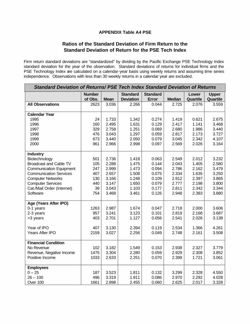
APPENDIX Table A4 PSE
Ratios of the Standard Deviation of Firm Return to the Standard Deviation of Return for the PSE Tech Index
Firm return standard deviations are “standardized” by dividing by the Pacific Exchange PSE Technology Index standard deviation for the year of the observation. Standard deviations of returns for individual firms and the PSE Technology Index are calculated on a calendar-year basis using weekly returns and assuming time series independence. Observations with less than 30 weekly returns in a calendar year are excluded.
Standard Deviation of Returns/ PSE Tech Index Standard Deviation of Returns Number
of Obs.
Mean Standard Deviation
Standard Error
Median
Lower Quartile
Upper Quartile
All Observations 2623 3.036 2.266 0.044 2.725 2.076 3.559 Calendar Year 1995 24 1.733 1.342 0.274 1.419 0.621 2.675 1996 160 2.495 1.631 0.129 2.417 1.141 3.468 1997 329 2.758 1.251 0.069 2.680 1.986 3.440 1998 476 3.043 1.297 0.059 2.817 2.173 3.727 1999 673 3.440 2.050 0.079 3.045 2.342 4.107 2000 961 2.966 2.998 0.097 2.569 2.026 3.164 Industry Biotechnology 501 2.736 1.418 0.063 2.549 2.012 3.232 Broadcast and Cable TV 105 2.288 1.475 0.144 2.043 1.405 2.580 Communication Equipment 247 2.999 1.473 0.094 2.786 2.162 3.479 Communication Services 407 2.657 1.508 0.075 2.334 1.635 3.250 Computer Networks 130 3.166 1.248 0.109 2.912 2.397 3.865 Computer Services 440 3.147 1.650 0.079 2.777 2.198 3.800 Cat./Mail Order (Internet) 39 3.043 1.103 0.177 2.811 2.342 3.344 Software 754 3.468 3.461 0.126 2.948 2.383 3.880 Age (Years After IPO) 0-1 years 1263 2.987 1.674 0.047 2.718 2.000 3.606 2-3 years 957 3.241 3.123 0.101 2.819 2.168 3.687 >3 years 403 2.701 1.127 0.056 2.541 2.026 3.138 Year of IPO 407 3.130 2.394 0.119 2.534 1.366 4.261 Years After IPO 2159 3.027 2.256 0.049 2.748 2.161 3.508 Financial Condition No Revenue 102 3.182 1.549 0.153 2.938 2.327 3.779 Revenue, Negative Income 1475 3.304 2.280 0.059 2.929 2.308 3.852 Positive Income 1033 2.633 2.251 0.070 2.399 1.721 3.061 Employees 0 – 25 187 3.523 1.811 0.132 3.299 2.328 4.550 26 – 100 496 3.319 1.911 0.086 2.970 2.292 4.028 Over 100 1661 2.898 2.455 0.060 2.625 2.017 3.328

APPENDIX Table A5 PSE
Correlations of Firm Returns to the Returns for the PSE Tech Index
Correlations are calculated on a calendar-year basis using weekly returns. Observations with less than 30 weekly returns in a calendar year are excluded.
Correlation with PSE Tech Index Number
of Obs.
Mean Standard Deviation
Standard Error
Median
Lower Quartile
Upper Quartile
All Observations 2623 0.234 0.356 0.007 0.280 0.099 0.452 Calendar Year 1995 24 -0.123 0.604 0.123 -0.093 -0.800 0.260 1996 160 0.000 0.542 0.043 0.155 -0.330 0.318 1997 329 0.148 0.336 0.019 0.175 0.046 0.312 1998 476 0.219 0.345 0.016 0.282 0.137 0.409 1999 673 0.079 0.339 0.013 0.133 -0.004 0.272 2000 961 0.426 0.206 0.007 0.447 0.308 0.576 Industry Biotechnology 501 0.206 0.319 0.014 0.232 0.073 0.381 Broadcast and Cable TV 105 0.218 0.324 0.032 0.243 0.114 0.417 Communication Equipment 247 0.277 0.360 0.023 0.288 0.124 0.525 Communication Services 407 0.261 0.347 0.017 0.320 0.131 0.469 Computer Networks 130 0.263 0.216 0.019 0.273 0.079 0.406 Computer Services 440 0.174 0.434 0.021 0.256 0.066 0.453 Catalog/Mail Order (Internet) 39 0.258 0.179 0.029 0.280 0.142 0.358 Software 754 0.254 0.359 0.013 0.295 0.123 0.481 Age (Years After IPO) 0-1 years 1263 0.182 0.451 0.013 0.268 0.055 0.470 2-3 years 957 0.256 0.220 0.007 0.256 0.114 0.406 >3 years 403 0.345 0.227 0.011 0.372 0.178 0.495 Year of IPO 407 0.000 0.659 0.033 0.199 -0.773 0.588 Years After IPO 2159 0.281 0.238 0.005 0.289 0.129 0.445 Financial Condition No Revenue 102 0.198 0.325 0.032 0.215 0.038 0.398 Revenue, Negative Income 1475 0.245 0.355 0.009 0.292 0.096 0.469 Positive Income 1033 0.227 0.354 0.011 0.273 0.114 0.433 Employees 0 – 25 187 0.138 0.304 0.022 0.141 0.029 0.305 26 – 100 496 0.197 0.353 0.016 0.242 0.057 0.406 Over 100 1661 0.271 0.325 0.008 0.307 0.145 0.472


![Venture Capital - Bird & Bird · Venture Capital One of the leading international law firms acting for investors and organisations disrupting, or being disrupted by ... [Struan] has](https://static.fdocuments.in/doc/165x107/5aeeeb837f8b9ac2468c004c/venture-capital-bird-bird-capital-one-of-the-leading-international-law-firms-acting.jpg)


