LBNL-6990E

Opportunities for Efficiency

Improvements in the U.S. Natural Gas

Transmission, Storage and

Distribution System

Jeffery B. Greenblatt

Energy Technologies Area

May 2015

This work was supported by the Office of Energy Policy and Systems Analysis (EPSA)

of the U.S. Department of Energy under Lawrence Berkeley National Laboratory

Contract No. DE-AC02-05CH11231

ERNEST ORLANDO LAWRENCE

BERKELEY NATIONAL LABORATORY

ii

DISCLAIMER

This document was prepared as an account of work sponsored by the United States

Government. While this document is believed to contain correct information,

neither the United States Government nor any agency thereof, nor The Regents of

the University of California, nor any of their employees, makes any warranty,

express or implied, or assumes any legal responsibility for the accuracy,

completeness, or usefulness of any information, apparatus, product, or process

disclosed, or represents that its use would not infringe privately owned rights.

Reference herein to any specific commercial product, process, or service by its

trade name, trademark, manufacturer, or otherwise, does not necessarily constitute

or imply its endorsement, recommendation, or favoring by the United States

Government or any agency thereof, or The Regents of the University of California.

The views and opinions of authors expressed herein do not necessarily state or

reflect those of the United States Government or any agency thereof, or The

Regents of the University of California.

Ernest Orlando Lawrence Berkeley National Laboratory is an equal opportunity

employer.

iii

Opportunities for Efficiency Improvements in the U.S. Natural Gas Transmission, Storage and Distribution System

Jeffery B. Greenblatt Lawrence Berkeley National Laboratory

Executive Summary This report provides an in-depth review of the U.S. natural gas transmission, storage and distribution system, from gas gathering at wellheads to final delivery to consumers, with a focus on energy efficiency opportunities. Drawing upon several resources published by the U.S. government and the natural gas industry, as well as a number of research papers and company publications, this report provides an overview of system components, historical and potential future trends, technical efficiency opportunities, cost estimates, and a final synthesis. While not comprehensive, a number of general conclusions can be drawn from the available information. There are a number of technical efficiency opportunities located throughout the natural gas infrastructure system that have yet to be fully realized. This includes improvements in compressors, prime movers (gas engines/turbines and electric motors), and capacity/operational choices; pipeline sizing, layout, cleaning, and interior coatings; and opportunities for waste heat recovery. While the natural gas gathering, processing, and transmission infrastructure being built as part of efforts to expand natural gas system capacity will generally be more efficient than existing natural gas infrastructure currently in place, there are opportunities to improve the efficiency of existing equipment (e.g. pipelines and compressor systems) through replacement and/or upgrades.

iv

Table of Contents Executive Summary............................................................................................................................................. iii Abbreviations ........................................................................................................................................................ vi 1. Overview .......................................................................................................................................................... 1

A. High-level description ........................................................................................................................... 1 B. Description of system components .................................................................................................. 2

i. Pipelines ................................................................................................................................................... 2 a. Transmission and Gathering ...................................................................................................... 2 b. Distribution ....................................................................................................................................... 5

ii. Compressor systems .......................................................................................................................... 6 a. Compressors ..................................................................................................................................... 6 b. Prime movers ................................................................................................................................ 11 c. Pairing of prime movers with compressors ...................................................................... 14 d. Preferred technologies by application ................................................................................ 14 e. Apportionment of compression systems ........................................................................... 15

iii. Storage and LNG .............................................................................................................................. 16 C. Historical and potential future trends .......................................................................................... 19

i. Natural gas supply and demand .................................................................................................. 19 ii. Compressor systems ....................................................................................................................... 21 iii. Pipelines ............................................................................................................................................. 22

a. Gathering systems ....................................................................................................................... 22 b. Transmission pipelines ............................................................................................................. 23 c. Distribution systems................................................................................................................... 25

iv. Storage and processing facilities ............................................................................................... 26 2. Technical efficiency opportunities ...................................................................................................... 26

A. Compressor systems ........................................................................................................................... 26 i. Compressors ........................................................................................................................................ 27 ii. Prime movers .................................................................................................................................... 30 iii. Combined systems.......................................................................................................................... 32 iv. Waste heat recovery ...................................................................................................................... 32

B. Pipelines ................................................................................................................................................... 33 i. Pipe diameter and gas pressure .................................................................................................. 33 ii. Pipe inspection and cleanliness .................................................................................................. 34 iii. Internal surface coatings ............................................................................................................. 34

C. Cost estimates ........................................................................................................................................ 35 i. Compressor systems ........................................................................................................................ 35 ii. Waste heat recovery ....................................................................................................................... 38 iii. Pipelines ............................................................................................................................................. 39 iv. Cleaning (pigging) ........................................................................................................................... 42 v. Internal coatings ............................................................................................................................... 42 vi. Storage, processing and LNG ...................................................................................................... 43

D. System-level trade-offs ...................................................................................................................... 43 3. Synthesis ....................................................................................................................................................... 46 Acknowledgments ............................................................................................................................................. 50 References ............................................................................................................................................................ 50

v

List of Tables Table 1. Trends in pipeline technology over time ................................................................................. 24 Table 2. Comparison of compressor technology efficiencies ............................................................ 29 Table 3. Heat rates of Caterpillar gas engines and turbines .............................................................. 30 Table 4. Relative driver/compressor cost comparison for a 14,400 hp unit.............................. 36 Table 5. Estimated pipeline installation costs. ....................................................................................... 39 Table 6. Cost comparison example for replacement of a 10,000 hp compressor ..................... 45 Table 7. Summary of efficiency opportunities in the U.S. natural gas TS&D system ............... 48 List of Figures Figure 1. Schematic overview of natural gas pipeline TS&D network ............................................. 2 Figure 2. Cumulative distribution of pipeline capacities in the U.S. in 2013: (a) normal scale

(b) log scale .................................................................................................................................................... 3 Figure 3. Major natural gas flows in the U.S. .............................................................................................. 4 Figure 4. Regional natural gas flows as of December 31, 2008 .......................................................... 5 Figure 5. Examples of (a) single-throw and (b) multi-throw centrifugal compressors ............ 7 Figure 6. Cut-away view of a single-stage centrifugal compressor ................................................... 8 Figure 7. Labyrinth seal of centrifugal compressor ................................................................................. 9 Figure 8. Cut-away view of an axial compressor ................................................................................... 10 Figure 9. Discharge pressure versus inlet flow for different compressor technologies ........ 10 Figure 10. Natural gas compressor station locations .......................................................................... 16 Figure 11. Weekly storage capacity in lower 48 states, December 1994-August 2014 ......... 17 Figure 12. Underground natural gas storage facilities as of 2010 .................................................. 18 Figure 13. LNG facilities for import and peaking ................................................................................... 19 Figure 14. Historical natural gas consumption in the U.S. ................................................................. 20 Figure 15. Age of U.S. natural gas transmission pipeline by decade .............................................. 25 Figure 16. Age of U.S. natural gas distribution pipeline by decade ................................................ 26 Figure 17. Compressor efficiency versus compression ratio for different compressor

technologies ................................................................................................................................................ 27 Figure 18. Thermal efficiency of gas turbines over time .................................................................... 31 Figure 19. Estimated and actual compressor cost breakdown for 2012–2013 ......................... 37 Figure 20. Estimated and actual total compressor costs vs. capacity for 2012–2013 ............ 38 Figure 21. Estimated and actual total pipeline costs vs. diameter for 2012–2013 .................. 40 Figure 22. Estimated and actual total pipeline cost trends, 2004–2013 ...................................... 41 Figure 23. Estimated and actual pipeline cost breakdown for 2012–2013 ................................ 42

vi

Abbreviations AGA, American Gas Association BGA, BlueGreen Alliance BPC, Bipartisan Policy Center Bscf, billion scf Btu, British thermal unit (~1,055 J) CAGI, Compressed Air and Gas Institute DC, direct current DOE, U.S. Department of Energy EPSA, Office of Energy Policy and Systems Analysis (an office within DOE) EIA, Energy Information Administration (an office within DOE) FERC, Federal Energy Regulatory Commission GHG, greenhouse gas HHV, higher heating value hp, horsepower (~746 W) INGAA, Interstate Natural Gas Association of America IUPAC, International Union of Pure and Applied Chemists LHV, lower heating value LNG, liquefied natural gas MAOP, maximum allowable operating pressure (of pipeline) Mhp, million horsepower (~746 MW) MMtCO2e, million metric tons of CO2 equivalent MMscf, million scf NARUC, National Association of Regulatory Utility Commissioners NETL, National Energy Technology Laboratory psi, pounds per square inch (~6,895 Pa) rpm, revolutions per minute RPS, renewable portfolio standard scf, standard cubic feet of gas (at 60°F and 14.73 psi). For natural gas, this is ~932 Btu LHV

or ~1,033 Btu HHV (the precise value depends on the composition of natural gas, which can vary). Mass density is ~20.86 g/scf (GREET, 2010).i

SMYS, specified maximum yield strength (of pipeline) SWRI, Southwest Research Institute TS&D, transmission, storage and distribution U.S., United States WHR, waste heat recovery

i Converted from conditions presented in GREET (2010) (0°C and 101.325 kPa; former IUPAC standard) by scaling values by 1.0545 scf per IUPAC ft3 (IUPAC, 1997).

1

1. Overview

A. High-level description

With the oldest long-distance pipeline completed in 1929, the U.S. natural gas transmission network is about 85 years old (INGAA, 2010a, p. 13), with ~320,000 miles (DOT, 2014a)1 of wide-diameter, high-pressure pipelines (EIA, 2008a). The distribution network constitutes the majority of pipeline distances (~2.15 million miles) (DOT, 2014b)2 and while it contains some legacy pipeline, is overall newer than the transmission network (EIA, 2014a). The modern natural gas transmission, storage and distribution (TS&D) infrastructure consists of a vast network of production wells, processing plants, pipelines, compressors, storage facilities and liquefaction plants, delivering about 73 Bscf of natural gas per day (~27,000 Bscf annually) in 2014. Seasonal demand varies between ~60 and ~100 Bscf/day (EIA, 2015a). Most natural gas that is consumed in the U.S. is produced domestically. About 10% is imported from Canada, with a very small portion imported from Mexico.3 The U.S. also exports a small percentage of its domestic production, resulting in net imports of 8% in 2011 (EIA, 2011) and ~4% projected for 2015 (EIA, 2015a). Overall, 99% of natural gas used in the U.S. is produced in North America (APGA, 2012). The EIA provides a useful schematic overview of the TS&D network, subdividing the system into gas gathering from production wells, gas processing, and imports; long-distance transmission pipelines; gas storage and LNG facilities (also mainly used for peaking storage); and distribution to end users (EIA, 2007; EIA, 2008b). Compression is used throughout the system (CAGI, 2012, p. 388; AGA, 2015a). See Figure 1. Except for the small amount of natural gas provided by LNG (EIA, 2015a), virtually all natural gas consumed is transported by pipeline; transport by rail or other vehicle is not considered economically feasible (INGAA, 2010b).

1 This total includes 17,000 miles of gathering pipelines: small-diameter pipelines that move natural gas from wells to processing plants or transmission interconnections (EIA, 2008a). 2 There is some confusion over what constitutes a distribution pipeline. DOT (2012, 2014b) breaks distribution into “mains” (distribution lines that serve as a common source of supply for more than one service line) and “service” (distribution lines that transport gas from a common source of supply, e.g., mains, to a customer meter or the connection to a customer's piping). Mains encompass ~1.25 million miles and service lines account for the remaining ~900,000 miles (DOT, 2014b). Both EIA (2014a) and BGA (2014) report 1.2 million miles of distribution pipelines, consistent with the DOT estimate for mains. It seems that the service portion of the distribution network was not included in the EIA and BGA definitions of “distribution.” 3 The U.S. imports from Mexico have been declining since 2007, reaching 0.3 Bscf in 2012 and 1.1 Bscf in 2013, as opposed to ~3,000 Bscf/yr from Canada between 2005-2013, though imports have been decreasing (EIA, 2014b).

2

Figure 1. Schematic overview of natural gas pipeline TS&D network Source: EIA (2008b)

The outline of this report is as follows. Section 1-B provides a detailed description of system components, while Section 1-C describes historical and potential future trends. Section 2 discusses technical opportunities for efficiency improvement in each part of the system, including costs (Section 2-C) and system-level trade-offs (Section 2-D). Finally, Section 3 provides a synthesis.

B. Description of system components

i. Pipelines

a. Transmission and Gathering

There are ~17,000 miles of small-diameter gathering pipelines that move natural gas from wells to processing plants or transmission interconnections (EIA, 2008a). There was very little additional information about natural gas gathering pipelines. The current high-pressure, inter- and intrastate transmission portion of the natural gas pipeline network consists of ~300,000 miles of pipelines organized into more than 210 individual pipeline systems (DOT, 2014a; EIA, 2007). As of 2008, about 70% of transmission pipeline mileage was interstate (EIA, 2008c). Pipe diameters range up to 48 inches and pressures vary between 200 and 1,750 psi (INGAA, 2010a, p. 18; CAGI, 2012, p. 423; AGA, 2015a; BPC, 2014). Approximately 27% of interstate pipeline diameters are 16 inches or smaller (EIA, 2008c). Pipeline flow rates vary tremendously, depending on what part of the delivery system is involved and local demand. Using flow rate capacities on ~530 individual pipelines in 2013 (EIA, 2014c), an analysis of the data indicates a range

3

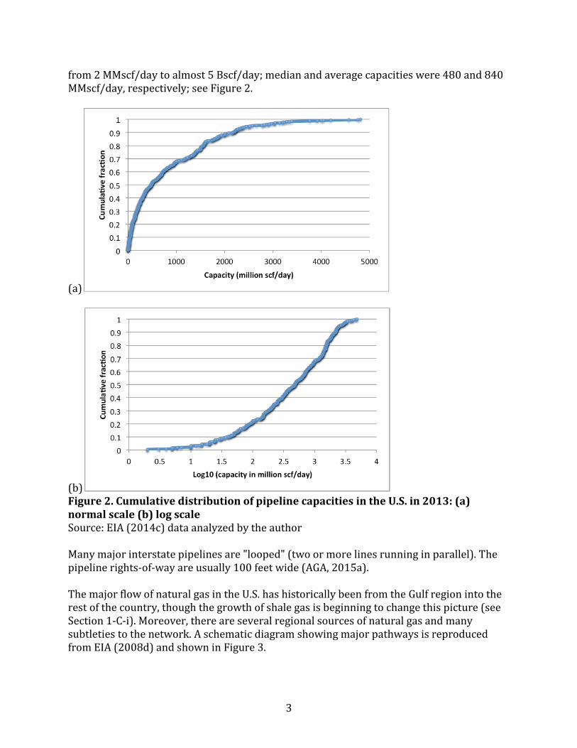
from 2 MMscf/day to almost 5 Bscf/day; median and average capacities were 480 and 840 MMscf/day, respectively; see Figure 2.

(a)

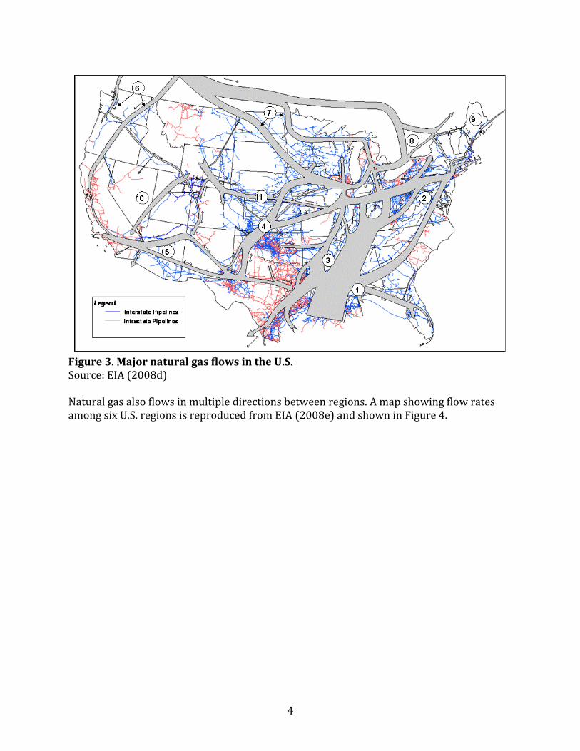
(b) Figure 2. Cumulative distribution of pipeline capacities in the U.S. in 2013: (a) normal scale (b) log scale Source: EIA (2014c) data analyzed by the author Many major interstate pipelines are "looped" (two or more lines running in parallel). The pipeline rights-of-way are usually 100 feet wide (AGA, 2015a). The major flow of natural gas in the U.S. has historically been from the Gulf region into the rest of the country, though the growth of shale gas is beginning to change this picture (see Section 1-C-i). Moreover, there are several regional sources of natural gas and many subtleties to the network. A schematic diagram showing major pathways is reproduced from EIA (2008d) and shown in Figure 3.

4

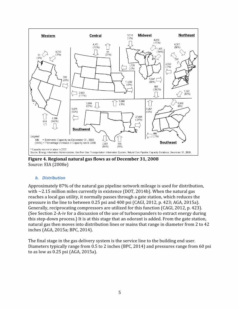
Figure 3. Major natural gas flows in the U.S. Source: EIA (2008d) Natural gas also flows in multiple directions between regions. A map showing flow rates among six U.S. regions is reproduced from EIA (2008e) and shown in Figure 4.

5

Figure 4. Regional natural gas flows as of December 31, 2008 Source: EIA (2008e)

b. Distribution

Approximately 87% of the natural gas pipeline network mileage is used for distribution, with ~2.15 million miles currently in existence (DOT, 2014b). When the natural gas reaches a local gas utility, it normally passes through a gate station, which reduces the pressure in the line to between 0.25 psi and 400 psi (CAGI, 2012, p. 423; AGA, 2015a). Generally, reciprocating compressors are utilized for this function (CAGI, 2012, p. 423). (See Section 2-A-iv for a discussion of the use of turboexpanders to extract energy during this step-down process.) It is at this stage that an odorant is added. From the gate station, natural gas then moves into distribution lines or mains that range in diameter from 2 to 42 inches (AGA, 2015a; BPC, 2014). The final stage in the gas delivery system is the service line to the building end user. Diameters typically range from 0.5 to 2 inches (BPC, 2014) and pressures range from 60 psi to as low as 0.25 psi (AGA, 2015a).

6

ii. Compressor systems

Compressor systems consist of two main components: the compressor itself and the prime mover (also called the compressor driver). There are several major technology options for each component, and the choice of components will depend upon trade-offs among multiple features.

a. Compressors

Major types of compressors are reciprocating, centrifugal and axial. (Other types of compressors exist as well but are not commonly used for natural gas compression). Reciprocating compressors work by compressing gas in a cylinder via piston movement. Capacities vary from fractional hp to more than 20,000 hp per unit. Pressures range from low vacuum at the inlet (or suction) side to 30,000 psi and higher at the discharge side. Reciprocating compressors come in two main configurations:

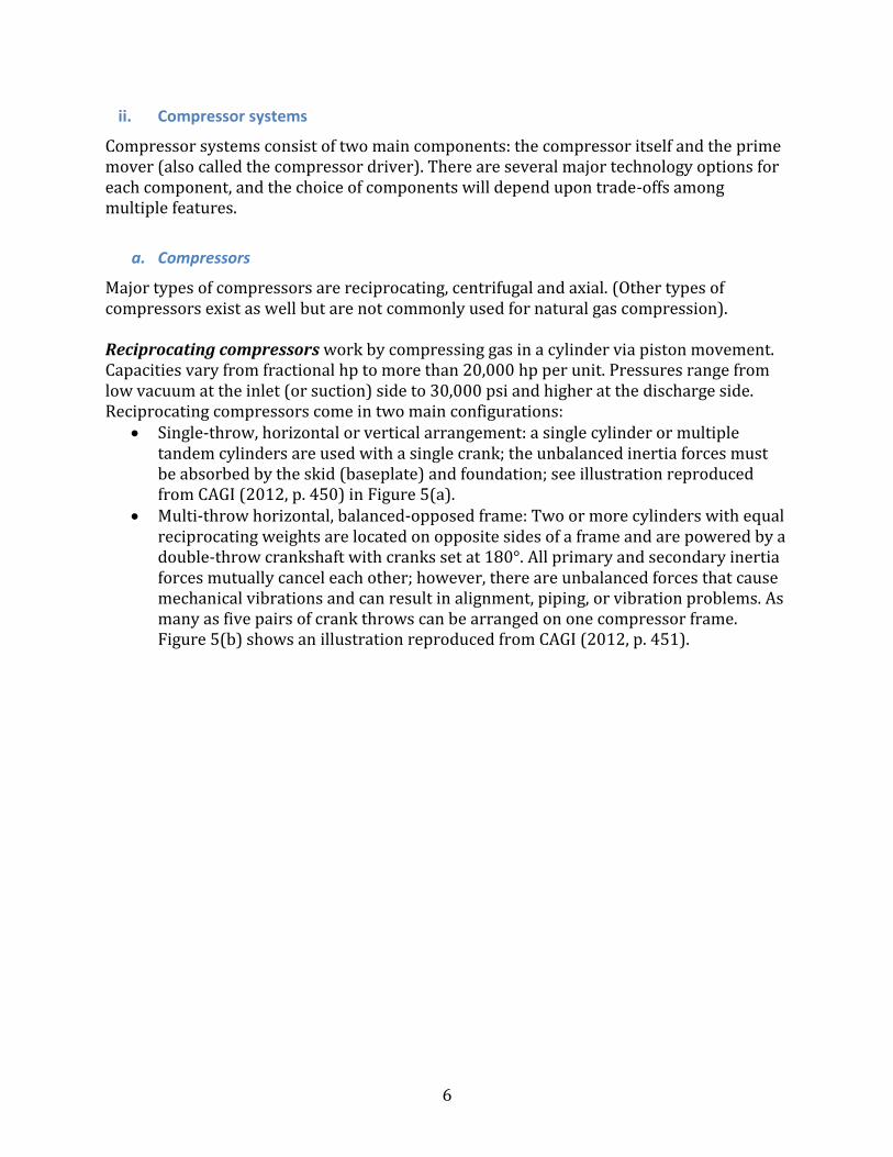
Single-throw, horizontal or vertical arrangement: a single cylinder or multiple tandem cylinders are used with a single crank; the unbalanced inertia forces must be absorbed by the skid (baseplate) and foundation; see illustration reproduced from CAGI (2012, p. 450) in Figure 5(a).

Multi-throw horizontal, balanced-opposed frame: Two or more cylinders with equal reciprocating weights are located on opposite sides of a frame and are powered by a double-throw crankshaft with cranks set at 180°. All primary and secondary inertia forces mutually cancel each other; however, there are unbalanced forces that cause mechanical vibrations and can result in alignment, piping, or vibration problems. As many as five pairs of crank throws can be arranged on one compressor frame. Figure 5(b) shows an illustration reproduced from CAGI (2012, p. 451).

7

(a)

(b) Figure 5. Examples of (a) single-throw and (b) multi-throw centrifugal compressors Source: CAGI (2012, pp. 450–451) Reciprocating compressors are built as either single- or multi-stage units. The number of stages is determined by the overall compression ratio. The compression ratio per stage (and valve life) is generally limited by the discharge temperature and usually does not exceed four, although small-sized units (used for intermittent duty) are furnished with a compression ratio as high as eight. On multi-stage machines, intercoolers (heat exchangers that remove the heat of compression from the gas, reducing the temperature to close to that of the compressor intake) are sometimes used between stages. Intercooling reduces the volume of gas going to the high-pressure cylinders, reducing the horsepower required for compression (CAGI, 2012, p. 474).

8

A centrifugal compressor uses the centrifugal force from a rotating gas flow to provide pressure to compress the gas. In its simplest form, a centrifugal compressor is a single-stage, single-flow unit with the impeller (the rotating part that imparts kinetic energy to the fluid) overhung on a motor CAGI (2012, p. 551); see the cut-away illustration reproduced from CAGI (2012, p. 552) shown in Figure 6. The gas enters the centrifugal compressor through the inlet nozzle (at right), which is proportioned to minimize turbulence as the gas enters the impeller. The rotating impeller (driven by an engine or motor) dynamically compresses the gas and also sets it in motion, giving it a velocity somewhat less than the tip speed of the impeller. The diffuser surrounds the impeller and serves to gradually reduce this velocity by increasing the pressure. A volute casing surrounds the diffuser and collects the gas, further reducing its velocity and further increasing the pressure. The gas exits at the top of the illustration (CAGI, 2012, p. 551).

Figure 6. Cut-away view of a single-stage centrifugal compressor Note: gas flow inlet is at right and outlet is at top. Source: CAGI (2012, p. 552) A multi-stage centrifugal compressor is a machine having two or more stages. Such compressors may be described as in-line (all impellers are on a single shaft and in a single casing) or integrally geared (impellers are mounted singly at one or both ends of each pin-

9

ion, and each impeller has its own separate casing). Integrally geared centrifugal compressors are normally used only on air and nitrogen service. Gas flow between stages is facilitated by inter-stage diaphragms, connecting the discharge of one impeller to the inlet of the next impeller. Sealing between stages is accomplished using labyrinth ring seals, which impose restriction on the flow between impellers at the shaft, at the impeller eye, and at the balancing drum (CAGI, 2012, pp. 545–552). An illustration of a labyrinth seal is reproduced from CAGI (2012, p. 595) in Figure 7.

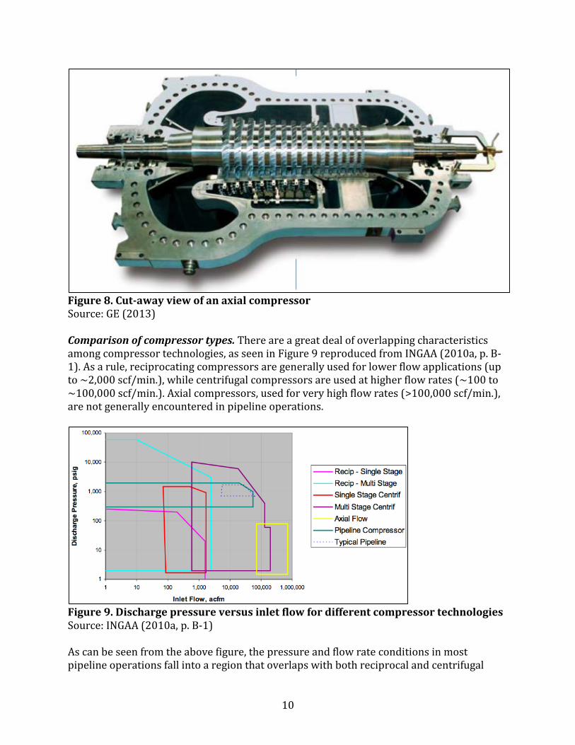
Figure 7. Labyrinth seal of centrifugal compressor Source: CAGI (2012, p. 595) Axial compressors are more reminiscent of gas turbines, compressing the gas through a series of rotating blades arranged along a common shaft; see reproduction from GE (2005, p. 13) in Figure 8. They are primarily used for low pressure, high-flow applications (INGAA, 2010a, p. B-1), and as such, are seldom used in the natural gas TS&D system except for producing LNG (GE, 2013, p. 5). They are characterized by roughly constant inlet flow over a considerable range of discharge pressure (CAGI, 2012, p. 559). Shaft-end seals can be labyrinth, oil films or dry, depending on service requirements (GE, 2013, p. 13).

10

Figure 8. Cut-away view of an axial compressor Source: GE (2013) Comparison of compressor types. There are a great deal of overlapping characteristics among compressor technologies, as seen in Figure 9 reproduced from INGAA (2010a, p. B-1). As a rule, reciprocating compressors are generally used for lower flow applications (up to ~2,000 scf/min.), while centrifugal compressors are used at higher flow rates (~100 to ~100,000 scf/min.). Axial compressors, used for very high flow rates (>100,000 scf/min.), are not generally encountered in pipeline operations.

Figure 9. Discharge pressure versus inlet flow for different compressor technologies Source: INGAA (2010a, p. B-1) As can be seen from the above figure, the pressure and flow rate conditions in most pipeline operations fall into a region that overlaps with both reciprocal and centrifugal

11

compressors. Among these two main types of compressors, reciprocating are more effective in situations with varying pressure ratios (i.e., where the ratio of discharge to suction pressure varies substantially), while centrifugal are more effective in situations with generally higher flow rates, some flow variability, and relatively constant pressure ratios. According to CAGI (2012, p. 474), the advantages of centrifugal over reciprocating compressors are:

Lower installed first cost where pressure and volume conditions are favorable Lower maintenance expense Greater continuity of service and dependability Less operating attention required Greater volume capacity per unit of plot area Adaptability to high-speed, low maintenance cost prime movers

Conversely, the advantages of reciprocating over centrifugal compressors (CAGI, 2012, p. 474) are:

Greater flexibility in capacity and pressure range Higher compressor efficiency and lower power cost Capability of delivering higher pressures Capability of handling smaller volumes Less sensitive to changes in gas composition and density

Differences in efficiency are discussed in Section 2-A.

b. Prime movers

Among prime movers, there are three main choices in use in the natural gas TS&D system: gas engines, gas turbines and electric motors. Gas engines. Similar to an internal combustion engine used in a vehicle, the gas engine (sometimes called a reciprocating engine) uses a chamber, filled with combusting natural gas, to drive a piston. While modern gas engines are quite efficient, they do have power limitations, and can have high vibration issues that affect reliability. Also, certain components may require frequent maintenance (INGAA, 2010a, p. 34). These issues are discussed more thoroughly in Sections 1-C-ii and 2-A. Gas engines are normally divided into two general categories related to speed. These categories are slow-speed engines (≤600 rpm) and medium-speed engines (600–2,100 rpm). There are also two basic types of gas engine designs: the two-stroke cycle and four-stroke cycle. Either type can be turbocharged. The two-cycle engines require less displacement for the same rating. The differences in performance between these engine types are small, especially with turbocharging (CAGI, 2012, p. 448). Slow speed engines are in common use in integral gas engine compressors. “Integral” indicates the use of a common crankshaft to drive both the power cylinders and the compressor. Integral machines are typically subdivided according to power output: small (25–800 hp) and large (800–7,000 hp). Small integral engines are used in oil field services

12

(gas gathering, gas injection, small gas processing plants). Larger integral engines are used in process plants, main line gas transmission, gas injection, and large gas plants (CAGI, 2012, p. 518). Medium-speed gas engines (600–2,100 rpm) are generally used for non-integral (separable) oil field compressors. Power sizes range from 5 to 3,600 hp, with the smaller end of the range (5–400 hp) generally operating at medium speed (1,400–1,800 rpm), while the larger end (300–3,600 hp) are generally directly connected and operate at lower speeds (600–1,200 rpm). Across the industry, the trend is toward higher driver speeds to keep pace with increasing compressor speeds (CAGI, 2012, p. 519). Legacy internal combustion, slow speed gas engines have significantly less sophisticated controls and lower fuel efficiencies than state-of-the-art engines (INGAA, 2010a, p. 34). Gas turbines use hot exhaust gases produced from the discharge of a gas generator to drive a power turbine. Two types of turbines are used: 1. aeroderivative engines, based on gas turbines developed for the aviation industry, and 2. industrial turbines, which are designed specifically for industrial use. Aviation industry developments have contributed to performance improvements in both types of turbines (INGAA, 2010a, p. 34). Gas turbines have limited application in the process and oil and gas industry as prime movers. The gas turbine is relatively new compared to the gas engine, steam turbine or electric motor (see Section 1-C-ii). However, there are some applications where gas turbines (typically driving reciprocating compressors) are more common. One application is offshore compression, where weight is a concern. Another application is refineries or process plants, where turbine exhaust heat can be utilized to improve overall plant efficiency (CAGI, 2012, p. 527). Smaller plants (<10,000 hp) will typically choose a gas engine over gas turbines, unless the waste heat can be utilized (see also discussion of waste heat recovery in Section 2-A-iv). Gas engines have inherently better efficiency compared to smaller gas turbines (CAGI, 2012, p. 435). Efficiency trade-offs will be discussed further in Section 2-A. Electric motors are more reliable and more efficient as stand-alone pieces of equipment than either gas engines or gas turbines. They are able to ramp up more rapidly than gas-driven prime movers. They also have an advantage where air quality regulations are an issue because they do not emit nitrogen oxides and CO2 at the point of use. There are a number of competing factors, however, that affect the suitability of electric motors over gas-based technology. One is the requirement for variable speed, while the other is the availability and proximity of a suitable electric power supply or substation. Reliability of the grid is also a concern, particularly in remote locations (INGAA, 2010a, pp. 34–35). While natural gas drivers are the primary technology for oil and gas field operations, electric motors are increasingly being used due to environmental considerations (CAGI, 2012, p. 520). There are three types of electric motors: induction, synchronous and DC. Each is described briefly below.

13

Induction is the most common type of electric motor. Induction motors generally have good efficiency and excellent starting torque, but rather high inrush current4 requirements. Induction motor efficiencies lie in the high 80% to low 90% range, depending on power. Smaller power induction motors are generally less efficient (CAGI, 2012, p. 522). Synchronous motors are the most common type of driver used for high-power applications, e.g., above 700 hp for speeds greater than about 450 rpm, or above 200 hp for lower speeds. These motors are typically more efficient than induction motors, with efficiencies in the range of 93%–97%. Synchronous motors must be carefully analyzed because of their lower torque characteristics, however (CAGI, 2012, pp. 521–522). The use of DC motors as oil field compressor drivers has increased in popularity in recent years. The reasons for this increase are threefold: 1. Availability of DC traction motors, 2. Variable-speed capability of DC motors to control compressor capacity, and 3. Economic considerations of motor drive versus engine drive. However, when utilizing DC motors in a hazardous atmosphere, it is necessary to provide a continuous positive air pressure in the motor enclosure to assure that no gas can get into the motor and be ignited. Offshore oil field compressors are using more DC motor drivers because of the added speed flexibility, lower initial cost, and projected lower maintenance costs (CAGI, 2012, p. 523). However, it appears that these are not used much in gas compression applications. The improvement in electronics control has greatly increased the potential for motors to be utilized as compressor drivers, especially in oil field applications. This has happened because of technological advances in motor controls. It is now economical to buy induction motors or synchronous motors with variable-speed controls to adjust the compressor operating speed. DC motors, having inherent variable-speed capability, already provide the needed variable speed with little further equipment needed. Variable speed to control compressor performance is a very desirable characteristic of a compressor prime mover (CAGI, 2012, p. 524). Other types of drivers include steam turbines, hydraulic turbines, and diesel or gasoline engines. All of these technologies are rarely used in the oil and gas industry. About these technologies, CAGI (2012, pp. 524–528) says:

Steam turbines are typically used to drive positive-displacement compressors where steam is available as a power source. However, it is generally not economical to use steam unless it is already available as part of a process, e.g., in refineries or natural gas processing plants.

A hydraulic turbine is like a centrifugal pump operating in reverse. This type of turbine is found in specialty situations where plentiful high-pressure liquid already exists, e.g., in a refinery or processing plant (as in the situation for steam turbines). “By decreasing the liquid pressure across the turbine, the pressure of the liquid is

4 Inrush current is the instantaneous current drawn by the motor when first turned on.

14

reduced to a desirable level and power is recovered. When high-pressure liquid is available, this type of driver offers essentially free energy” (CAGI, 2012, p. 528).

Diesel engines are used infrequently in the oil and gas industry, but there are some applications where they are economical, such as “air drilling compressors, kick-off compressors (used to start an oil field gas lift), fire floods, or standby compressors” (CAGI, 2012, p. 525). Also, there are dual-fuel configurations that allow the operator to select the most economical fuel (diesel or natural gas).

Gasoline engines are also used rarely because of high fuel costs. They are primarily used with standby compressors. Operating and application characteristics of gasoline engines resemble those of natural gas and diesel engines.

c. Pairing of prime movers with compressors

Compressor selection usually dictates the choice of the prime mover. Gas engines are generally limited to driving reciprocating compressors, while gas turbines generally drive centrifugal compressors. Electric motors, on the other hand, may be used with either compressor technology, and pipeline companies have begun using electric motors to power centrifugal compressors on a more widespread basis than reciprocating compressors (INGAA, 2010a, p. 35).

d. Preferred technologies by application

Gathering systems typically need one or more field compressors (AGA, 2015a). Compressors are used to provide suction to lift gas from underground reservoirs, with inlet pressures ranging from 25 to 65 psi and discharge pressures from 800 to 1,200 psi. Compression is also used to reinject gas into reservoirs to maintain pressure, with discharge pressures from 3,000 to 4,000 psi (CAGI, 2012, pp. 421–423). CAGI estimates that gas-gathering applications account for the majority of installed reciprocating compressor capacity in the oil and gas industry; however, some centrifugal technology is used in low-pressure applications. Gas compression for lift service is typically utilized where electricity is not practical or economical, and gas is readily available (CAGI, 2012, p. 422). Oil and gas field applications require compressor systems that are compact and can be easily moved from one location to another. The normal drivers for these compressors are coupled gas engines or electric motors. These units are called “separables” (CAGI, 2012, pp. 447). Pipeline evacuation involves the transfer of gas from a static section of pipeline to an active section of pipeline. This is accomplished by reciprocating compressors that can handle wide variation in suction pressures while compressing against a constant discharge pressure. Packaged compressor systems specifically designed for this application feature multiple compression stages that can maintain high driver loading throughout a wide range of compression ratios. Most such units are driven by gas engines. Typical conditions are intake pressures ranging from 850 psi initially, down to a final pressure of 50 psi, and a constant discharge pressure of 850 psi (CAGI, 2012, p. 424).

15

For gas storage, the compressor must not only be able to handle filling the reservoir but also the return of the gas. This dual service requires operating pressure flexibility and is provided best by the reciprocating compressor. Typical pressure conditions are suction from 35 to 600 psi during injection, 300 to 800 psi during withdrawal, and discharge from 600 to 4,000 psi during the injection phase and 700 to 1,000 psi as the gas is withdrawn from the reservoir and fed to the transmission line (CAGI, 2012, p. 425). Reciprocating compressors are also often used to increase the pressure of the gas used as fuel for operating engines or turbines, known as fuel gas boosting. Suction pressures range from 10 psi (e.g., landfill gathering systems) to 50 psi (refinery or utility distribution headers), and discharge pressures range from 40 psi (engines) to 400 psi (turbines) (CAGI, 2012, pp. 427–428). Compressor requirements for gas processing plants vary widely depending on the type and size of the plant (100–1,000 MMscf/day) and the composition of the gas stream. Performance flexibility and plant energy balance are much more important than first cost when determining the type of compression to be used. Larger plants tend to use centrifugal compressors with turbines, either gas or steam, as drivers. Large-capacity and relatively stable gas conditions make the choice of centrifugal compressors practical on the basis of efficiency and installed cost. Internal combustion engines powered with natural gas typically used as prime movers, though environmental (mainly air quality) concerns are causing electric motors to become more prevalent (CAGI, 2012, pp. 433–434).

e. Apportionment of compression systems

In terms of prime mover technology, the natural gas industry operated over 6,000 gas engines, 1,000 gas combustion turbines, and 200 electric motors in 2010 (INGAA, 2010a, p. 42), though Hedman (2008) notes that electric motor populations may be growing quickly. The average capacity of a gas engine is 1,700 hp, while gas turbines tend to be much larger (6,600 hp on average) (Hedman, 2008), with electric motors being even larger (average of 7,800 hp) (Boss, 2015). Large (>15,000 hp) gas turbines account for >25% of total gas turbine capacity, even though they constitute <9% of total units. Based on data in Hedman (2008), gas engines represent about 60% of total prime mover capacity (expressed in hp), with the balance supplied overwhelmingly by gas turbines. ICF (2009) contains historical compressor additions back to 1999 and projected additions through 2030, and indicates that between 2010 and 2013, capacity grew by ~1.8 million hp (Mhp). Putting these data together, it is estimated that total compressor capacity in 2013 was 20.2 Mhp.5 The actual number of compressor stations is far fewer than the number of compressor units, because multiple units typically are grouped at a single compressor station (INGAA, 2010a, p. 42). There are more than 1,400 compressor stations that maintain pressure on

5 Average capacity of electric motors was unknown but estimated to be similar to gas turbines. The 2009 reference capacity was calculated as (6,000 engines x 1,700 hp) + (1,000 turbines x 6,600 hp) + (200 motors x 7,800 hp) = 18.4 Mhp, based on INGAA (2010a, p. 42). Additions between 2010-2013 (ICF, 2009) bring the total estimate to 20.2 Mhp.

16

the natural gas pipeline network and assure continuous forward movement of supplies (EIA, 2007). About 2.4% of compressor units are electric-drive, but these constitute ~5% of total compressor horsepower (Boss, 2015). Multiple compressors are increasingly common at larger compressor capacities (e.g., >1,000 hp) (FERC, 2014). Figure 10 reproduces the EIA map of compressor station locations (EIA, 2008f).

Figure 10. Natural gas compressor station locations Source: EIA (2008f) Based on data from 2004 (Hedman, 2008) and 2010 (INGAA, 2010a), much of the gas engine capacity is quite old, with ~45% having been in service for more than 50 years, an additional ~15% installed before 1970, ~20% installed between 1970 and 1990, and the remaining ~20% installed since 1990.6 Information on the distributions of gas turbines and electric motors was not available, but they are both newer additions to the TS&D system (see Section 1-C-ii).

iii. Storage and LNG

There are more than 400 underground storage facilities for natural gas (EIA, 2010). Total working gas storage capacity has increased from ~4,200 Bscf in 2008 to ~4,750 Bscf in 2013 (EIA, 2015b). Gas in storage undergoes strong seasonal and, to a lesser extent,

6 Values in text have been adjusted to reflect a ~10% growth in gas engine capacity between 2004 and 2010 (INGAA, 2010a, p. 42).

17

interannual variability; see Figure 11.7 In recent years, the low point typically occurs in winter at around 1,500 Bscf, but in March 2014, it dipped to 822 Bscf (EIA, 2014d). However, a high level of storage injection brought supplies back to reasonable levels (~2,700 Bscf as of August 29, 2014) (EIA, 2014d).

Figure 11. Weekly storage capacity in lower 48 states, December 1994-August 2014 Source: EIA (2014d) data analyzed by the author A map of storage facilities as of 2010 is provided by EIA and reproduced in Figure 12 (EIA, 2010).

7 EIA has data extending back to 1949, providing a useful picture of interannual supply variation (EIA, 2011).

18

Figure 12. Underground natural gas storage facilities as of 2010 Source: EIA (2010) There are 12 LNG regasification terminals as of August 15, 2014 (FERC, 2015a) and over 100 LNG peaking facilities (used to supplement stored natural gas during high demand periods) (EIA, 2008g); see Figure 13. A number of new LNG facilities are planned; see Section 1-C-i for a discussion.

19

Figure 13. LNG facilities for import and peaking Source: EIA (2008g). Note that four additional LNG import terminals have been added since publication of this map (see text and FERC, 2015a). In addition to the dedicated storage facilities described above, natural gas companies routinely raise and lower the pressure in pipeline segments to achieve short-term gas storage during periods when there is less demand at the end of the pipeline. This technique is called “line packing” and may allow pipeline operators to meet higher demand for short durations (AGA, 2015a).8 Sometimes this involves raising the capacity of a line above its rated capacity, but pressure remains within safety limits (EIA, 2007).

C. Historical and potential future trends

i. Natural gas supply and demand

Demand for natural gas has increased steadily over time, but went through a period of dramatic growth from the mid-1930s to late 1960s, growing from 1,500 Bscf/yr in 1933 to 20,000 Bscf/yr in 1969, and has remained roughly at this level through the mid-2000s (EIA, 2001; EIA, 2014e). See Figure 14. Subsequently, demand began to grow again with the development of horizontal drilling and hydraulic fracturing technologies that have enabled

8 “Line pack” is the inventory of gas in a pressurized section of a pipeline network (NWGA, 2012). It is the volume of gas that must be maintained within the line at all times in order to maintain pressure and insure an uninterrupted flow of transportation of natural gas through the pipeline. Line packing is not a substitute for traditional underground gas storage facilities and pipeline operations.

20

the U.S. to economically extract hydrocarbon resources from unconventional shale gas reservoirs. Total domestic natural gas production was about 23,000 Bscf/yr (63 Bscf/day) in 2011 (EIA, 2011), and reached a record high of 77 Bscf/day in November 2014, in step with growing demand (EIA, 2015a). Under INGAA auspices, ICF (2014) published a projected expansion of U.S. natural gas production of 40 Bscf/day between 2014 and 2035 (and 3.0 Bscf/day from Canada).9 Most of this U.S. expansion (23 Bscf/day) is expected by 2020. Total consumption for natural gas (including exports of 5 Bscf/day to Mexico and 9 Bscf/day as LNG) is projected to grow to 120 Bscf/day by 2035.

Figure 14. Historical natural gas consumption in the U.S. Sources: EIA (2001) and EIA (2014e) data analyzed by the author As stated earlier in Section 1-A, most natural gas is produced within the U.S., with about 15% imported from Canada, and about 5% is exported. However, the rise in shale gas is causing large changes in the natural gas industry: not just growth in demand, but also dramatic shifts in how pipelines are utilized. Some existing natural gas transmission pipelines are reversing flow, while new pipelines are being rerouted to accommodate gas supplies on newly-constructed pipelines, as shale gas supplies are often not located in North America’s most prolific supply basins. The increasing competition between natural gas supply basins and demand regions is changing the direction of natural gas flows on pipeline infrastructure across the country. According to NARUC, “the rapid growth of shale gas production redraws the map for pipeline flows across North America” (Honorable, 2012). Increasing shale gas production, and in turn comparatively low U.S. natural gas prices, has led to interest in exporting LNG. As of February 5, 2015, five U.S. export facilities have been approved and are under construction, with total capacity of 9.2 Bscf/day (FERC, 2015b). An

9 In addition, ICF (2014) projects 3.1 Bscf/day of natural gas liquids capacity will be added in the U.S. between 2014 and 2035, and 0.5 Bscf/day in Canada, roughly doubling current production.

0

5,000

10,000

15,000

20,000

25,000

30,000

1930 1950 1970 1990 2010

Na

tura

l G

as

Co

nsu

mp

tio

n (

Bsc

f/y

r)

21

additional 14 U.S. sites have been proposed to FERC (FERC, 2015c) and there are 13 more potential sites identified by project sponsors (FERC, 2015d). However, ICF (2014) projects that LNG export capacity will expand by only 9.3 Bscf/day by 2035, with a low-growth case projecting only 4.0 Bscf/day. DOE is in the midst of changing its framing of the approval process for LNG export terminals (DOE, 2014; Rosner, 2014). While no site currently under consideration has a capacity larger than 3.2 Bscf/day, the DOE is currently assessing how the construction of larger LNG export facilities (between 12 and 20 Bscf/day) would affect the public interest (DOE, 2014). It also released a life-cycle assessment of the GHG impacts of exporting LNG to other countries to displace coal for electricity generation, concluding that while LNG has lower life-cycle GHG emissions than coal, the details of the results depend on assumptions (NETL, 2014).

ii. Compressor systems

Note: Information on compressor systems (compressors plus prime movers) was mainly limited to one data source: INGAA (2010a). Additional sources of data, including details on compressor system age, capacity, manufacturer, efficiency, technology type, etc. would be extremely useful. The current network includes 30- to 50-year-old “legacy” compressor engines that are “relatively large, robust, and slow speed (300 rpm) machines designed to operate continuously for years without a shutdown” (INGAA, 2010a, p. 12). The use of these older compressors has declined with increases in steel and construction costs. After World War II, the system expanded substantially due to advances in metallurgy, steel pipe, welding techniques and compressor technology (INGAA, 2010a, pp. 12-13). In the 1950s, the main compressor technology was a slow-speed “integral” reciprocating compressor where a single design encompassed compressor and gas engine, producing smaller, more compact systems with lower installation costs. Centrifugal compressors driven by gas turbines began to dominate the market in the 1960s and 1970s, because they cost less to install and maintain than integral reciprocating compressors. Pipeline companies could also purchase large centrifugal units at significant cost savings compared to purchasing multiple smaller (reciprocating) compressor units (INGAA, 2010a, pp. 13-15). Electric motors began to be used with larger, reciprocating compressors in the 1990s. Although technology enabling high power, high voltage, variable speed systems became available in the 1980s, synchronous and induction motor technology and variable-frequency drive systems did not emerge until the late 1990s (INGAA, 2010a, p. 16). However, the majority of engine technology is still gas-driven (see Section 1-B-ii-e). Reciprocating compressors reemerged in the 1990s for low-flow applications with the development of high-speed systems that became available at lower cost. High-speed internal combustion gas engines were developed to match these compressors and offered

22

higher thermal efficiencies and thus lower fuel usage than older, low-speed systems (INGAA, 2010a, p. 16). New technology has not come without a cost. Vibration and pulsation problems cause a number of maintenance issues. Researchers at SWRI have been developing solutions to these problems, such as a tapered cylinder nozzle to reduce vibration and boost efficiency, and a semi-active electromagnetic plate valve to extend valve life roughly 10-fold. As compressor valves are the single largest maintenance cost item for reciprocating compressors, this improvement appears to be a significant advance (Deffenbaugh et al., 2005). Since 2005, SWRI won an R&D Magazine “R&D100” award for this technology (SWRI, 2007) and a patent was filed in 2010 (US Patent Office, 2010). As of 2013, total compressor capacity (of all types) was ~20 Mhp (see Section 1-B-ii-e) and near-term planned expansion totaled 450,000 hp (Smith, 2013a). ICF’s (2014) projected compressor capacity expansion between 2014 and 2035 estimated an additional 12.8 Mhp would be required,10 with 66% of this capacity attributed to natural gas gathering, and the remainder to transmission pipelines. Total compressor capacity is therefore likely to grow to ~29-33 Mhp by 2035. In addition, 661,000 hp of compression would be needed to transport natural gas liquids (ICF, 2014).

iii. Pipelines

The natural gas network consists of ~2.5 million miles of pipeline, of which 320,000 miles are large diameter, high-pressure gathering and transmission pipelines, while the remainder (~87%) are distribution pipelines. About 142,000 miles of the current transmission network were installed in the 1950s and 1960s, as natural gas demand exploded following World War II. A large portion of the 2.15 million miles of local distribution pipelines was also installed in the same period. However, the greatest growth in the local distribution network occurred in the 1990s during a period of low prices, where more than 225,000 miles of new distribution pipelines were installed to provide natural gas to many new residential and commercial facilities (DOT, 2014a, 2014b; EIA, 2014a, 2014f).

a. Gathering systems

Almost no information was available about pipelines for natural gas gathering, other than total mileage: ~11,000 miles onshore and ~6,000 miles offshore (DOT, 2014a). DOT (2012) provides an age distribution for natural gas transmission and gathering pipelines combined, which is almost identical to data provided by Kiefner and Rosenfeld (2012) (see Section 1-C-iii-b). From this data, it appears that the distribution of natural gas gathering pipeline ages is similar to that of the natural gas transmission network.

10 ICF (2014) also explored a low demand case with only 8.9 Mhp of compressor expansion by 2035. The older ICF (2009) study made even lower projections, estimating an expansion of between 2.5 and 6.5 Mhp through 2030 (after subtracting estimated Canadian additions of 0.8-1.3 Mhp).

23

ICF (2014) projects that an additional 303,000 miles of gathering lines will be needed between 2014 and 2035, greatly expanding current capacity. The average diameter of these new lines is 3.6 inches. 11

b. Transmission pipelines

As noted previously, the oldest long-distance pipeline in the U.S. was completed in 1929 (INGAA, 2010a, p. 13), marking the genesis of the modern natural gas network. Since the 1950s, the general practice has been to build pipelines using the combination of pipeline diameter and compression to transport gas for the lowest delivered cost, but not necessarily at the highest efficiency (INGAA, 2010a, p. 13). “Beginning in the 1960s, improved metallurgy and manufacturing practices permitted the construction of larger diameter pipeline with higher strength steel to transport natural gas longer distances at higher operating pressures with less compression and at lower costs. Pipeline companies also began experimenting with new, higher cost, internal coating technology that reduced friction” (INGAA, 2010a, p. 14); this is discussed in more detail in Section 2-B-iii. Accompanying the growth in natural gas demand has been the construction since 1996 of more than 34,000 miles of new natural gas transmission pipeline, representing more than 200 Bscf/day of capacity (EIA, 2014g)—about three times the total current demand of ~73 Bscf/day; see Section 1-A. Most growth supported access to new supply sources such as imports from Canada, expanding production from new shale gas fields, and increased demand from new natural-gas-fired electric power plants. Most trunk expansions were on the order of 1 Bscf/day, though there were some significantly larger local expansions, including Canadian gas pipelines (2.6 Bscf/day), the Gulf offshore region (~5 Bscf/day), projects in the Powder River, Green River, Piceance, and Unitah basins of Wyoming, Colorado, and Utah to access coal-bed methane and tight-sands natural gas production (more than 14 Bscf/day), and new intrastate headers and laterals (6 Bscf/day) (EIA, 2008h). More recent major pipeline projects on the horizon (2015 onward) amount to 81 Bscf/day and 9,145 miles (EIA, 2014g). ICF (2014) projects that new transmission pipeline requirements will amount to 18,600 miles between 2014 and 2035. An additional 17,100 miles of “laterals to/from power plants, storage field and processing plants” is projected, as well as 15,100 miles of transmission for natural gas liquids. Diameters of long-distance transmission pipelines have increased steadily over the years, with maximum diameters of 24 inches in the oldest pipelines and up to 48 inches since 2000 (INGAA, 2010a, p. 19). As noted in Section 1-B-a, as of 2008, only 27% of interstate pipelines had diameters of 16 inches or less. The increase in pipe diameter has been

11 ICF (2014) reports 1,095,000 inch-miles and 303,100 miles of gathering lines; the quotient gives average diameter. Similar calculations were used for calculating average diameter of mainlines, laterals and natural gas liquids transmission (see Section 1-C-iii-b).

24

accompanied by increases in maximum allowable operating pressures (MAOP) from 720 psi in pre-1950 pipelines to more than a doubling to 1,750 psi today. This has been achieved through the development of high strength steels, enabling pipelines to be built and operated at higher pressures economically. As shown in Table 1 reproduced from INGAA (2010a, p. 19), available pipeline steel specified maximum yield strengths (SMYS) have increased from 42,000 psi before 1940 to 100,000 psi in 2010. Advances in steel strength continue to this day. Also, improved quality control in manufacturing, transportation, installation and testing of new pipe has allowed the operating pressure of some new pipe installations to increase from 72% to 80% of its SMYS (INGAA, 2010a, p. 18). Table 1. Trends in pipeline technology over time

Source: INGAA (2010a, p. 19) Based on author calculations of data from (ICF, 2014), projected expansion between 2014 and 2035 indicates an average pipe diameter for new transmission lines of 30.5 inches, and 16.3 inches for laterals. BPC (2014) reports on materials comprising transmission pipelines. About 97% of pipeline miles consists of cathodically protected, coated steel,12 with other steels (cathodically unprotected, uncoated or both) comprising ~2.5%. The remaining portion (~0.4%) is mainly plastic. Pipeline ages were reported by an INGAA Foundation-sponsored report (Kiefner and Rosenfeld, 2012) based on DOT data provided in 2009. Approximately 60% of pipeline

12 According to BPC (2014), “Proper coating on the exterior of steel pipelines inhibits the reaction of the metal with its environment, and cathodic protection imparts a direct current to the pipeline to further prevent the corrosion process.” Surface coating typically uses fusion-bond epoxy; older systems used coal tar epoxy. A direct current can be achieved through the use of a sacrificial material such as magnesium, which has a different electrochemical potential than steel, as well as through an applied external voltage (INGAA, 2010b).

25

miles are at least 45 years old, with almost 50% built between 1950 and 1969. See Figure 15 for more details.

Figure 15. Age of U.S. natural gas transmission pipeline by decade Source: Kiefner and Rosenfeld (2012)

c. Distribution systems

Distribution pipelines are constructed from a variety of materials, including various types of steel, cast iron, plastic (mainly polyethylene), and copper, though plastic has become the material of choice over the past 30 years (DOT, 2011; AGA, 2015b; BGA, 2014; BPC, 2014), comprising 52-54% of the ~1.25 million miles of distribution mains pipelines (BGA, 2014; BPC, 2014).13 Advantages of plastic pipe include flexibility, corrosion resistance, and low installation cost—particularly because it can often be inserted into existing lines or through soil without the trenching that is often required for other materials (AGA, 2015b). Protected coated steel is the second most common material, comprising nearly 40% of distribution pipeline miles. The remaining ~9% consists of cast or wrought iron (~3%),14 bare steel (~5%) and unprotected coated steel (~1%) (BGA, 2014; BPC, 2014). According to BGA (2014), this latter ~9% constitutes the most leak-prone portion of the distribution network, while BPC (2014) puts this number at closer to 7%. Although the portion of leak-prone miles fell 43% between 1990 and 2011, these materials are estimated to be 18 times more leak-prone than plastic and 57% more leak-prone than treated steel (BGA, 2014).

13 BPC (2014) also estimated that distribution service lines consist of 68.7% plastic, 21.5% cathodically protected, coated steel, 3.4% bare steel, 2.4% unprotected, coated steel, 1.4% copper and 2.4% other. 14 The iron pipe was built more than 50 years ago (DOT, 2012; BGA, 2014).

26

The age profile of distribution system is given by decade from DOT (2012) in Figure 16. Compared to transmission pipeline ages, the ages of distribution pipelines are much younger, with nearly 70% less than 45 years old.

Figure 16. Age of U.S. natural gas distribution pipeline by decade Source: DOT (2012)

iv. Storage and processing facilities

Little data were available on natural gas storage and processing facilities. ICF (2014) projected expansion of working gas storage by 823 Bscf between 2014 and 2035 (current capacity is ~4,800 Bscf; see Section 1-B-iii). ICF (2014) also projected increases in natural gas processing facility capacity of 34.2 Bscf/day between 2014 and 2035, nearly as large as projected growth in production (~40 Bscf/day).

2. Technical efficiency opportunities

A. Compressor systems

As partly covered in Section 1-B-ii, compressor systems vary in efficiency depending on choice of compressor and prime mover technology, power, speed, compression ratio and load factor. Moreover, the most efficient compressor is often not the most economical

27

choice from the perspective of the pipeline company. Costs and cost trade-offs are discussed in Section 2-C.

i. Compressors

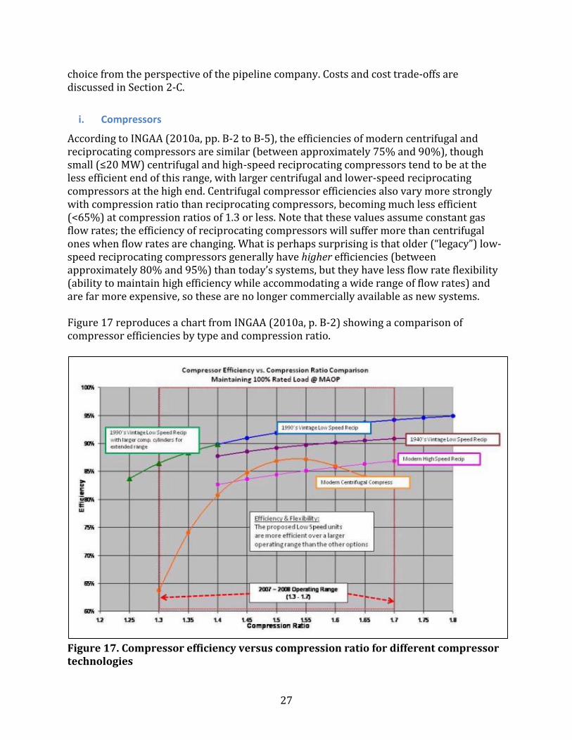
According to INGAA (2010a, pp. B-2 to B-5), the efficiencies of modern centrifugal and reciprocating compressors are similar (between approximately 75% and 90%), though small (≤20 MW) centrifugal and high-speed reciprocating compressors tend to be at the less efficient end of this range, with larger centrifugal and lower-speed reciprocating compressors at the high end. Centrifugal compressor efficiencies also vary more strongly with compression ratio than reciprocating compressors, becoming much less efficient (<65%) at compression ratios of 1.3 or less. Note that these values assume constant gas flow rates; the efficiency of reciprocating compressors will suffer more than centrifugal ones when flow rates are changing. What is perhaps surprising is that older (“legacy”) low-speed reciprocating compressors generally have higher efficiencies (between approximately 80% and 95%) than today’s systems, but they have less flow rate flexibility (ability to maintain high efficiency while accommodating a wide range of flow rates) and are far more expensive, so these are no longer commercially available as new systems. Figure 17 reproduces a chart from INGAA (2010a, p. B-2) showing a comparison of compressor efficiencies by type and compression ratio.

Figure 17. Compressor efficiency versus compression ratio for different compressor technologies

28

Source: INGAA (2010a, p. B-2) INGAA also provides a table detailing a wide variety of compressor-prime mover combinations and characteristics, with efficiency estimates of each component as well as overall system efficiency under design conditions; this is reproduced in Table 2 (INGAA, 2010a, p. B-5).

29

Table 2. Comparison of compressor technology efficiencies

Source: INGAA (2010a, p. B-5)

30

According to CAGI (2012, p. 478), energy losses from valves (see Section 1-C-ii) in high-speed (≥1000 rpm) compressors can be as much as 20%, suggesting that improvements in valve performance may have a significant impact on efficiency. As mentioned in Section 1-C-ii, SWRI researchers successfully demonstrated a proof-of-concept approach to reducing energy losses arising from vibration and pulsation in high-speed reciprocating compressors by about 6% (Deffenbaugh at all, 2005). The same authors claimed that overall compressor efficiencies of 90% can now be achieved, and expressed optimism for increasing the efficiency of slow-speed compressors to as much as 95%. For reciprocating compressors, compressor cylinder can be replaced with improved designs that are rated for higher pressures or designed to accommodate changes in load. The pulsation control system can also be modified to increase efficiency. Both of these are retrofit opportunities that do not require replacing the compressor (INGAA, 2010a, p. 41).

ii. Prime movers

Laurenzi and Jersey (2013, pp. 26–27) analyzed heat rates of gas prime movers manufactured by Caterpillar, reporting mean heat rates and standard deviations of both gas engines and turbines. See Table 3. The range of capacities spanned by this data is very large: 95 to 8,180 hp15 (Caterpillar, 2014). Laurenzi and Jersey (2013) also examined data from Siemens, reporting that efficiencies were similar in both mean value and variation. Table 3. Heat rates of Caterpillar gas engines and turbines

Technology Mean heat

rate Standard deviation

Mean efficiency

(calculated)

Standard deviation of efficiency (calculated)

Btu/hp-hr (HHV) % (HHV) Gas engines 6,825 38.7 37.28 0.21 Gas turbines 8,772 797 29.01 2.65 Source: Laurenzi and Jersey (2013) Dividing the standard deviation by the mean efficiency gives one estimate of the efficiency

improvement potential for gas prime movers, resulting in 0.6% for gas engine technology, and 9.1% for gas turbine technology. However, these estimates may be overly conservative, as INGAA (2010a, p. 19) claimed enormous improvement in recent years among large (>20,000 hp) gas turbines, from 27% to 40% thermal efficiency (9,426 to 6,362 Btu/hp-hr). Smaller turbines have seen similar efficiency improvements, but operate slightly less efficiently (approximately 31% to 38%—see Figure 18) than the largest turbines. Note that the smaller (<10,000 hp) turbine efficiency data stops in 2000. As stated in Section 1-B-ii-e, Hedman (2008) reported that large (>15,000 hp) gas turbines account for >25% of total gas turbine capacity.

15 Some references use the notation “bhp” (brake horsepower) while others simply use “hp” (horsepower). According to the American Heritage Dictionary (2013), bhp is the “actual or useful horsepower of an engine, usually determined from the force exerted on a friction brake or dynamometer connected to the drive shaft.” However, the terms bhp and hp are interchangeable (Bruzek, 2008).

31

Figure 18. Thermal efficiency of gas turbines over time Source: INGAA (2010a, p. 19). Note: Chart was modified to correct mislabeled legend. “Small” is defined as <10,000 hp; “large” is >10,000 hp. Engine controls can be added to increase thermal efficiency in some older gas engines. Also, a gas engine can be replaced with an electric motor to accommodate a wider throughput range more efficiently (through speed variation) than other techniques (INGAA, 2010a, p. 41). Electric motor efficiency is far higher, between ~90% and 97% (CAGI, 2012, p. 522), with the upper end corresponding to synchronous motors. However, it is difficult to compare electric motor efficiency with that of gas-based technology (INGAA, 2010a, p. B-5), because one must consider efficiencies of motor, transmission (6% on average; EIA, 2014h) and electricity production (for natural gas, this ranges from 40% to 60%; COSPP, 2010) as a system, and electricity can also be made using non-combustion methods, such as hydropower, wind or solar. INGAA estimates that system efficiency for electric motors varies between 25% and 46% (INGAA, 2010a, p. B-5). Even if system efficiency is lower than that of natural gas, electric motors may have lower GHG emissions if the GHG intensity of the generated electricity is sufficiently low. However, the choice of electric vs. gas may be increasingly driven by air quality concerns (INGAA, 2010a, p. 24). Electric motors do appear to be a more efficient choice than gas engines when flow rates vary substantially (see Section 1-ii-b).

Small Turbines

Large Turbines

32

iii. Combined systems

For combined systems (prime mover plus compressor), for gas turbine-driven centrifugal compressors, the overall design efficiency of new systems has increased 50% since ca. 1990, and is now close to 33%. Gas engine-driven reciprocating compressors have improved as well: since 1995, their overall efficiency has increased from 42%–46% at peak thermal efficiency (100% load) (INGAA, 2010a, p. 20), representing a ~10% improvement. Moreover, it is becoming more common to power high horsepower, low speed, reciprocating compressors (80%–92% efficiency) with either gas engines (30–43% efficiency) or electric motors (90%–97% efficiency),16 to improve overall compressor system efficiency (INGAA, 2010a, p. 20).

iv. Waste heat recovery

INGAA published a pair of reports (Hedman, 2008, 2009) documenting technical and economic opportunities for waste heat recovery from natural gas TS&D systems. Three types of heat recovery options were considered:

Waste heat recovery from prime mover exhaust in compressor systems Use of turboexpanders (compressors “run in reverse”) to recover energy during gas

expansion to lower pressure, usually when gas enters the distribution network Inlet air cooling to increase turbine efficiency in hot weather

The reports found that waste heat recovery from compressor systems is economical under certain circumstances, but the other two options did not appear to be viable under current economic conditions.17 The economic opportunity for waste heat recovery is much greater for gas turbines than gas engines, because of the higher temperature and larger quantity of heat available in turbine exhaust. However, economically viable opportunities are currently limited to large systems (≥15,000 hp) with high annual load factors (>60%). About 90–100 compressor stations in the U.S. were identified as meeting these criteria, representing a potential of 500–600 MW in generation capacity (Hedman, 2008). This potential represents ~10% of gas compressor turbine capacity and 4%–5% of total gas compressor prime mover capacity, but a small fraction (~0.2%) of U.S. gas-based power generation (EIA, 2014i). As of November 2009, eight waste heat recovery projects have been installed on pipeline gas turbine compressor drivers in the U.S., with seven more in Canada; together these provide about 75 MW of electric generating capacity. Ten more projects are planned, with four in the U.S. representing an additional 22.5 MW. All projects are located in states with an RPS program or other incentive to favor waste heat recovery (Hedman, 2009). These

16 Note caveats about comparing electric and gas efficiencies; see Section 2-A-ii. 17 Turboexpanders have been successfully installed in LNG and gas processing plants, where they are sometimes economical, but outside of this, only four demonstration plants were built in the 1980s representing a total of 3.8 MW capacity, but all were deemed uneconomical and eventually shut down. Turbine inlet air cooling appears to suffer from a net efficiency penalty, and so does not make economic sense at present (Hedman, 2008).

33

programs tend to increase the value of electricity sold by 0.5–1.0 ¢/kWh, which is a significant increment over the typical wholesale electricity price of 3.5–5.0 ¢/kWh (Hedman, 2008). All projects have also been installed on gas turbine compressors (Hedman, 2009).

B. Pipelines

i. Pipe diameter and gas pressure

Viewed in equivalent energy terms and equivalent transport distances, natural gas pipelines consume an average of 2%–3% of throughput to overcome frictional losses (INGAA, 2010a, p. 1). To improve the hydraulic efficiency of their systems, pipeline companies use the largest diameter pipelines and highest pressures possible while still being cost-effective (INGAA, 2010a, p. 18). Doubling the pipeline diameter will allow four times the gas flow with virtually the same operating cost (INGAA, 2010a, p. A-2), while conversely, doubling the gas flow in a fixed-diameter pipe will quadruple the energy needed to compress it (INGAA, 2010a, p. 28). While not explicitly stated in the above sources, it appears that the energy required by compressors scales with the inverse fourth power of pipe diameter for a fixed flow rate. This conclusion is consistent with standard engineering texts (e.g., Lindeburg, 2011) as well as equations specific to the natural gas industry (Coelho and Pinho, 2007; Brikić, 2011), some forms of which suggest that the scaling relationship may be even stronger, e.g., inverse fifth power of pipe diameter. However, other limiting factors (e.g., economics) must come into play as pipe diameter increases, so that the maximum diameter used by the pipeline industry today (48 inches) presumably represents an economic balance point. Nonetheless, it may be worth exploring whether significant increases in energy cost (e.g., through a price on carbon) could push the industry to adopt larger pipe diameters than those used in current practice in order to reduce compressor fuel usage. This may particularly be the case for smaller-diameter pipelines. This point will be reiterated in Section 3. As discussed in Section 1-C-iii, significant improvements have been possible through advancements in materials and compressor technology. New trunk pipelines are typically built with a larger diameter pipe than will be needed initially, but with compression capacity limited to meeting current needs, as compressors can be added later (either at new or existing stations) to increase capacity as demand increases (EIA 2007). Increasing the MAOP increases gas throughput and reduces compressor fuel consumption, increasing efficiency. The Department of Transportation’s Pipeline and Hazardous Materials Safety Administration determines the MAOP of pipelines (INGAA, 2010a, p. 39).

34

ii. Pipe inspection and cleanliness

In the 1980s, companies expanded the use of advanced pipeline maintenance and inline inspection (ILI) technologies to clean and inspect the pipeline wall (“pigging”),18 further reducing friction (INGAA, 2010a, pp. 14–19). Recently, there has also been an effort to “digitize” the pipeline network, providing real-time information on gas flows, leaks, and hazards through various types of sensors (including those mounted on wheeled or airborne robotic platforms), data analytics, visualization and advanced simulation (Accenture, 2014a). On September 8, 2014 GE and Accenture jointly announced their “industrial internet” solution for better pipeline management, to be implemented within the Marcellus and Utica shale gas production regions (Accenture, 2014b). The emphasis of these efforts is on increasing reliability and safety, reducing operational costs, and prevention of and/or rapid recovery from failures. A gain in efficiency from better system operation, or having a smoother interior surface is a side-benefit (Roberts, 2009a). For cleaning, both mechanical (dry) scrubbing as well as a variety of liquid (surfactant, acid, gel) methods can be used. A combination of mechanical and liquid cleaning is generally considered superior. However, quantitative data on efficiency improvement from cleaning are lacking, though the claim is that liquid-based cleaning “should more than pay for itself” (Roberts, 2009b). Additionally, shorter and straighter lengths of pipe, and avoidance of obstacles such as valves and flow meters in the pipeline (INGAA, 2010a, p. A-1 to A-2), as well as removal of debris such as “hard hats, wooden skids, pig bars, chill rings, welding rods, and electric grinders” (Roberts, 2009a) that are occasionally left in pipelines, will increase efficiency. As discussed in Section 1-C-iii-c, replacing leak-prone pipes in the distribution network would save 23 Bscf/yr (BGA, 2014), or ~0.1% of total natural gas consumption. Such repairs would also have important safety and reliability benefits.

iii. Internal surface coatings

As noted in Section 1-C-iii, pipeline companies began experimenting with internal coatings to reduce friction and increase system efficiency in the 1960s; however, internally coated pipes only became widely available starting in the 1990s.19 The use of internal coatings has, according to one coatings manufacturer, become “standard industry practice” (Jotun, 2014). Others similarly claim that internal coatings are becoming “widely applied in gas pipelines and a remarkable economic benefit has been achieved” (Deyuan et al., 2011); many European countries and China have adopted coating technologies, with dramatic 18 “Legend has it they are called pigs because the early internal cleaning devices were made a [sic] leather cover stuffed with batting materials which made a sound much like a pig as line pressure pushed the device through the line. Maintenance pigs come in a variety of configurations including elastomeric spheres or devices consisting of a mandrel with elastomeric cups, discs, pigs, and brushes fastened to it. Some even have magnets to attract iron sulfide (rust)” (INGAA, 2010b). 19 There are a variety of coating materials available, including fusion bond epoxy coatings (INGAA, 2010a, p. 30), but there was no additional information available in the references examined on the chemical composition of these coatings.

35

improvements in gas transmission rates, in some cases up to 30% (Deyuan et al., 2011). However, the U.S. is curiously absent from the list, suggesting the practice may be less widespread here. Internal coatings are most effective at high flow rates, where flow is often turbulent. However, for a sufficiently low surface roughness, a laminar film can be formed at the pipe wall-fluid interface, reducing friction between the fluid and the pipe with a concomitant reduction in pressure drop and reduced amount of power needed to maintain pressure at a given throughput. An internal coating can form a more even coating on the inner pipe wall, reducing surface roughness (INGAA, 2010a, p. 30; Collet and Chizet, 2013). Typical values of average absolute roughness (maximum peak to valley height) for uncoated steel pipe are 20–50 µm (with the latter corresponding to corroded pipe) and 1–5 µm for coated pipe (Deyuan et al., 2011; Collet and Chizet, 2013). INGAA provided an example of an 11% reduction in fuel use compared to bare steel pipe when using an internal coating (INGAA, 2010a, p. C-1). Other researchers have reported increased flow rates between 5% and 27% (Pipelines International, 2011; Collet and Chizet, 2013), so coatings can make a significant impact on efficiency. A reduction in compression power can therefore be achieved with the same gas flow rate (Collet and Chizet, 2013). A new innovation is the use of microgrooves to further reduce friction below that which can be achieved simply by making an internal surface as smooth as possible. Initially explored in the 1970s by Michael Walsh at NASA Langley, this so-called biomimetic drag-reducing coating “…completely broke through the traditional way of thinking,” and has recently been realized experimentally by a group at Beijing University (Deyuan et al., 2011). Using a groove of 135 µm width and 100 µm height on a coated surface that already possessed very low (5.5 µm) surface roughness, a further improvement of 6% in gas transport efficiency was achieved (Deyuan et al., 2011).

C. Cost estimates

Cost data was difficult to obtain and only a handful of data points were available. More detailed information on the costs of various system components and their cost trade-offs are critically needed to help evaluate efficiency opportunities.

i. Compressor systems

While slow speed, integral reciprocating compressors are typically more efficient than modern high-speed compressors, they are “…generally no longer commercially available because they are cost-prohibitive to manufacture and install,” (Deffenbaugh et al., 2005). The trend has been toward larger, more flexible machinery that can handle large swings in gas flow rates necessary in modern operations. Therefore, a return to earlier technology appears infeasible. “Assuming the same configuration and location, two smaller compressor units will have a higher cost per horsepower compared to a larger unit due to economies of scale,” (INGAA, 2010a, p. 32).

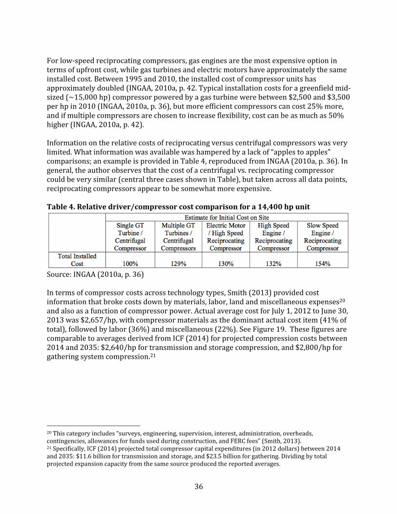
36

For low-speed reciprocating compressors, gas engines are the most expensive option in terms of upfront cost, while gas turbines and electric motors have approximately the same installed cost. Between 1995 and 2010, the installed cost of compressor units has approximately doubled (INGAA, 2010a, p. 42. Typical installation costs for a greenfield mid-sized (~15,000 hp) compressor powered by a gas turbine were between $2,500 and $3,500 per hp in 2010 (INGAA, 2010a, p. 36), but more efficient compressors can cost 25% more, and if multiple compressors are chosen to increase flexibility, cost can be as much as 50% higher (INGAA, 2010a, p. 42). Information on the relative costs of reciprocating versus centrifugal compressors was very limited. What information was available was hampered by a lack of “apples to apples” comparisons; an example is provided in Table 4, reproduced from INGAA (2010a, p. 36). In general, the author observes that the cost of a centrifugal vs. reciprocating compressor could be very similar (central three cases shown in Table), but taken across all data points, reciprocating compressors appear to be somewhat more expensive. Table 4. Relative driver/compressor cost comparison for a 14,400 hp unit

Source: INGAA (2010a, p. 36) In terms of compressor costs across technology types, Smith (2013) provided cost information that broke costs down by materials, labor, land and miscellaneous expenses20 and also as a function of compressor power. Actual average cost for July 1, 2012 to June 30, 2013 was $2,657/hp, with compressor materials as the dominant actual cost item (41% of total), followed by labor (36%) and miscellaneous (22%). See Figure 19. These figures are comparable to averages derived from ICF (2014) for projected compression costs between 2014 and 2035: $2,640/hp for transmission and storage compression, and $2,800/hp for gathering system compression.21

20 This category includes “surveys, engineering, supervision, interest, administration, overheads, contingencies, allowances for funds used during construction, and FERC fees” (Smith, 2013). 21 Specifically, ICF (2014) projected total compressor capital expenditures (in 2012 dollars) between 2014 and 2035: $11.6 billion for transmission and storage, and $23.5 billion for gathering. Dividing by total projected expansion capacity from the same source produced the reported averages.

37

Figure 19. Estimated and actual compressor cost breakdown for 2012–2013 Source: Smith (2013). Total compressor cost vs. capacity (in hp) is shown in Figure 20, where a downward trend with increasing hp is evident. Data for individual compressor projects in 2012–2013 (Smith, 2013) exhibit considerably more variability than these averages, however.

38

Figure 20. Estimated and actual total compressor costs vs. capacity for 2012–2013 Source: Author calculations using data from Smith (2013)

ii. Waste heat recovery

As discussed in Section 2-A-iv, waste heat recovery from compressor systems can sometimes be economical. Hedman (2008) estimated that the capital cost of such systems on large (>15,000 hp) gas turbines is $2,000–$2,500/kW.22 With reasonable assumptions about equipment life and financing,23 the annualized capital cost is about 3.1 ¢/kWh, on top of which an additional 0.5 ¢/kWh is added to pay the pipeline operator for the value of the heat, and an additional ~0.2 ¢/kWh is added to pay for operations and maintenance (range: 0.1–0.5 ¢/kWh). Given that current prices for wholesale power range between 3.5–5.0 ¢/kWh for long-term (20–30 year) purchase agreements, such systems can be favorable when capacity factors are sufficiently high. Green incentives (~0.5–1.0 ¢/kWh) can create a strong additional financial incentive (Hedman, 2008). Although deemed uneconomical under current circumstances, the report did estimate capital costs for turboexpander systems as well: between $600 and $2,300/kW (in 1987 dollars), with the lower figure reflecting the considerable economy of scale inherent for a larger system (3.8 MW). Operational costs are also high: in addition to fuel for gas heating, the maintenance of the turboexpander is estimated to be 0.1–0.5 ¢/kWh (Hedman, 2008).

22 Hedman (2009) updated this estimate to $2,500-3,500/kW. However, the 2008 values are retained here in order to provide a consistent calculation. 23 Assumptions: 20-year equipment life, 8% financing and 95% capacity factor; lower capacity factors will drive up cost considerably (Hedman, 2008).

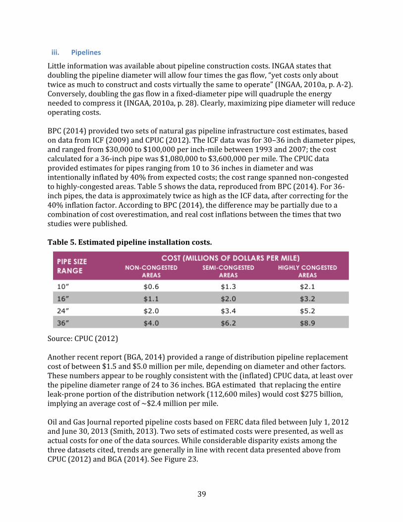
39

iii. Pipelines

Little information was available about pipeline construction costs. INGAA states that doubling the pipeline diameter will allow four times the gas flow, “yet costs only about twice as much to construct and costs virtually the same to operate” (INGAA, 2010a, p. A-2). Conversely, doubling the gas flow in a fixed-diameter pipe will quadruple the energy needed to compress it (INGAA, 2010a, p. 28). Clearly, maximizing pipe diameter will reduce operating costs. BPC (2014) provided two sets of natural gas pipeline infrastructure cost estimates, based on data from ICF (2009) and CPUC (2012). The ICF data was for 30–36 inch diameter pipes, and ranged from $30,000 to $100,000 per inch-mile between 1993 and 2007; the cost calculated for a 36-inch pipe was $1,080,000 to $3,600,000 per mile. The CPUC data provided estimates for pipes ranging from 10 to 36 inches in diameter and was intentionally inflated by 40% from expected costs; the cost range spanned non-congested to highly-congested areas. Table 5 shows the data, reproduced from BPC (2014). For 36-inch pipes, the data is approximately twice as high as the ICF data, after correcting for the 40% inflation factor. According to BPC (2014), the difference may be partially due to a combination of cost overestimation, and real cost inflations between the times that two studies were published. Table 5. Estimated pipeline installation costs.

Source: CPUC (2012) Another recent report (BGA, 2014) provided a range of distribution pipeline replacement cost of between $1.5 and $5.0 million per mile, depending on diameter and other factors. These numbers appear to be roughly consistent with the (inflated) CPUC data, at least over the pipeline diameter range of 24 to 36 inches. BGA estimated that replacing the entire leak-prone portion of the distribution network (112,600 miles) would cost $275 billion, implying an average cost of ~$2.4 million per mile. Oil and Gas Journal reported pipeline costs based on FERC data filed between July 1, 2012 and June 30, 2013 (Smith, 2013). Two sets of estimated costs were presented, as well as actual costs for one of the data sources. While considerable disparity exists among the three datasets cited, trends are generally in line with recent data presented above from CPUC (2012) and BGA (2014). See Figure 23.

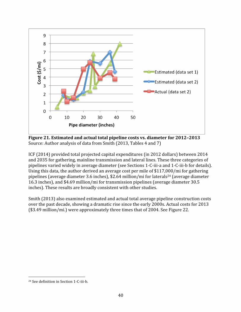
40

Figure 21. Estimated and actual total pipeline costs vs. diameter for 2012–2013 Source: Author analysis of data from Smith (2013, Tables 4 and 7) ICF (2014) provided total projected capital expenditures (in 2012 dollars) between 2014 and 2035 for gathering, mainline transmission and lateral lines. These three categories of pipelines varied widely in average diameter (see Sections 1-C-iii-a and 1-C-iii-b for details). Using this data, the author derived an average cost per mile of $117,000/mi for gathering pipelines (average diameter 3.6 inches), $2.64 million/mi for laterals24 (average diameter 16.3 inches), and $4.69 million/mi for transmission pipelines (average diameter 30.5 inches). These results are broadly consistent with other studies. Smith (2013) also examined estimated and actual total average pipeline construction costs over the past decade, showing a dramatic rise since the early 2000s. Actual costs for 2013 ($3.49 million/mi.) were approximately three times that of 2004. See Figure 22.

24 See definition in Section 1-C-iii-b.

41

Figure 22. Estimated and actual total pipeline cost trends, 2004–2013

Source: Smith (2013). Note: While there were sometimes large annual differences between estimated and actual costs, the overall trends of both are significantly upward. Finally, as for compressors, Smith (2013) provides a cost breakdown for compressor construction by component. Labor constitutes the most significant (47%) component of actual cost, followed by miscellaneous (31%) and materials (16%). See Figure 23.

42

Figure 23. Estimated and actual pipeline cost breakdown for 2012–2013 Note: ROW = rights-of-way (land). Source: Smith (2013)

iv. Cleaning (pigging)

No useful cost information was available about pigging for efficiency improvement, other than the claim that liquid-based cleaning “should more than pay for itself” (Roberts, 2009b). There is also a cost distinction between “online” (pipeline continues to operate) versus “offline” (pipeline out of service and depressurized) pigging. “As a rule, offline cleaning can be twice as expensive as online and the cost is compounded by the loss of gas revenues,” (Roberts, 2009a). Pigging costs are higher offline due to a number of factors: slower pig velocity, more cleaning runs, the need for pressurized nitrogen and air to propel the cleaning equipment, and the fuel cost to generate pressurization over the duration of cleaning. In the case where natural gas at low pressure can be used as a propellant, some cost savings may be realized (Roberts, 2009a).

v. Internal coatings

According to INGAA, because it involves a substantial expense, internal coatings are not cost-effective in many circumstances (for instance, at light load capacities). When coatings are economically justified, they are most often used for future expansions, pipeline replacements or as a trade-off against the expense of higher compressor power (INGAA, 2010a, p. 30).

43

INGAA provides a cost estimate range of between $2–$8/ft. depending on pipe diameter and type of coating (INGAA, 2010a, p. C-1), though coating materials other than fusion bond epoxy were not specified. If the factory producing the pipe is unable to coat it, it must be shipped to another location for coating, costs could be higher and possibly result in construction delays. According to INGAA, replacing old steel pipe with new, internally coated pipe would typically be cost prohibitive because efficiency gains would not justify the cost (INGAA, 2010a, p. C-1). Fogg and Morse (2005) provided a few cost estimates that consist of a mixture of absolute and relative values. One study they cited reported savings of $20 million for a 530 km length pipe with a flow of 5.6 MMscf/day; the pipe diameter was not specified. Another study reported 5% cost savings due to a reduction in pipe diameter from 26 to 24 inches (outer diameter) while using the same compressors to achieve the same flow. A third study calculated cost savings of 7%–14% relative to uncoated steel pipe with little corrosion (20 µm roughness), increasing to 15%–25% savings when the pipe was heavily corroded (50 µm roughness). Collet and Chizet (2013) provided even more optimistic estimates of cost savings, citing a 2002 examine from Argentina where a 1,200 km length of coated pipe incurred 27% lower compressor costs than uncoated pipe, among the highest savings cited in the literature. The source goes on to claim that reduced energy costs from internal coatings often have a financial payback of 3-5 years, with even further savings possible if the number of compressor stations and/or compressor capacity is reduced. For the microgrooved pipe coating with an estimated efficiency improvement of 6%, the researchers estimate that the cost of such a coating is (Chinese) ¥10 (about $1.60) per m2 of internal pipe surface (Deyuan et al., 2011). Using their assumed internal diameter of 40 inches, this translates into $5,100/km or $1.55/ft. of pipe distance.

vi. Storage, processing and LNG

Only one source of information was available to estimate costs of new natural gas storage, processing and LNG plants: ICF (2014). This source provided total projected capital expenditures (in 2012 dollars) in these categories between 2014 and 2035, along with projected capacity additions (see Sections 1-C-i and 1-C-iv). By dividing these two quantities, average costs per unit of capacity were obtained:

Natural gas storage: $14.6 million per Bscf Natural gas processing plant: $801 million per Bscf/day LNG export facility: $4.70 billion per Bscf/day

D. System-level trade-offs

Note: All information in this section comes from a single industry source (INGAA, 2010a). Additional sources of information or perspective would be useful to verify and update this information in the future.

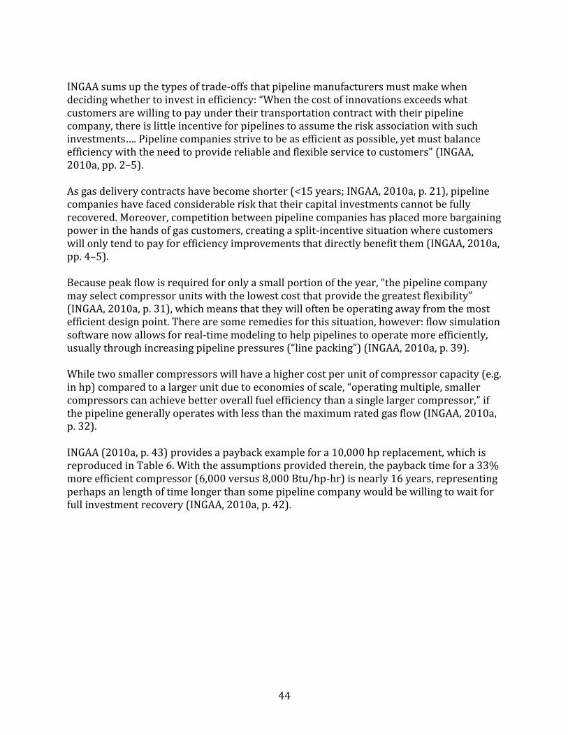
44

INGAA sums up the types of trade-offs that pipeline manufacturers must make when deciding whether to invest in efficiency: “When the cost of innovations exceeds what customers are willing to pay under their transportation contract with their pipeline company, there is little incentive for pipelines to assume the risk association with such investments…. Pipeline companies strive to be as efficient as possible, yet must balance efficiency with the need to provide reliable and flexible service to customers” (INGAA, 2010a, pp. 2–5). As gas delivery contracts have become shorter (<15 years; INGAA, 2010a, p. 21), pipeline companies have faced considerable risk that their capital investments cannot be fully recovered. Moreover, competition between pipeline companies has placed more bargaining power in the hands of gas customers, creating a split-incentive situation where customers will only tend to pay for efficiency improvements that directly benefit them (INGAA, 2010a, pp. 4–5). Because peak flow is required for only a small portion of the year, “the pipeline company may select compressor units with the lowest cost that provide the greatest flexibility” (INGAA, 2010a, p. 31), which means that they will often be operating away from the most efficient design point. There are some remedies for this situation, however: flow simulation software now allows for real-time modeling to help pipelines to operate more efficiently, usually through increasing pipeline pressures (“line packing”) (INGAA, 2010a, p. 39). While two smaller compressors will have a higher cost per unit of compressor capacity (e.g. in hp) compared to a larger unit due to economies of scale, “operating multiple, smaller compressors can achieve better overall fuel efficiency than a single larger compressor,” if the pipeline generally operates with less than the maximum rated gas flow (INGAA, 2010a, p. 32). INGAA (2010a, p. 43) provides a payback example for a 10,000 hp replacement, which is reproduced in Table 6. With the assumptions provided therein, the payback time for a 33% more efficient compressor (6,000 versus 8,000 Btu/hp-hr) is nearly 16 years, representing perhaps an length of time longer than some pipeline company would be willing to wait for full investment recovery (INGAA, 2010a, p. 42).

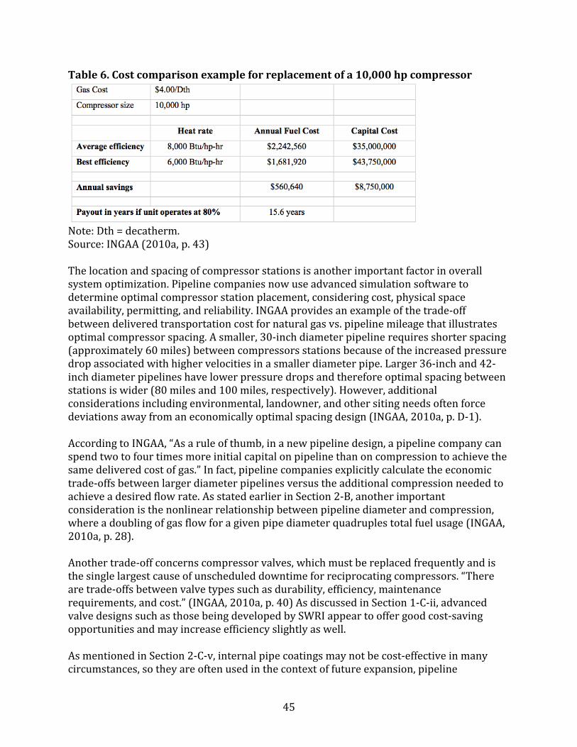
45

Table 6. Cost comparison example for replacement of a 10,000 hp compressor

Note: Dth = decatherm. Source: INGAA (2010a, p. 43) The location and spacing of compressor stations is another important factor in overall system optimization. Pipeline companies now use advanced simulation software to determine optimal compressor station placement, considering cost, physical space availability, permitting, and reliability. INGAA provides an example of the trade-off between delivered transportation cost for natural gas vs. pipeline mileage that illustrates optimal compressor spacing. A smaller, 30-inch diameter pipeline requires shorter spacing (approximately 60 miles) between compressors stations because of the increased pressure drop associated with higher velocities in a smaller diameter pipe. Larger 36-inch and 42-inch diameter pipelines have lower pressure drops and therefore optimal spacing between stations is wider (80 miles and 100 miles, respectively). However, additional considerations including environmental, landowner, and other siting needs often force deviations away from an economically optimal spacing design (INGAA, 2010a, p. D-1). According to INGAA, “As a rule of thumb, in a new pipeline design, a pipeline company can spend two to four times more initial capital on pipeline than on compression to achieve the same delivered cost of gas.” In fact, pipeline companies explicitly calculate the economic trade-offs between larger diameter pipelines versus the additional compression needed to achieve a desired flow rate. As stated earlier in Section 2-B, another important consideration is the nonlinear relationship between pipeline diameter and compression, where a doubling of gas flow for a given pipe diameter quadruples total fuel usage (INGAA, 2010a, p. 28). Another trade-off concerns compressor valves, which must be replaced frequently and is the single largest cause of unscheduled downtime for reciprocating compressors. “There are trade-offs between valve types such as durability, efficiency, maintenance requirements, and cost.” (INGAA, 2010a, p. 40) As discussed in Section 1-C-ii, advanced valve designs such as those being developed by SWRI appear to offer good cost-saving opportunities and may increase efficiency slightly as well. As mentioned in Section 2-C-v, internal pipe coatings may not be cost-effective in many circumstances, so they are often used in the context of future expansion, pipeline

46

replacement, or as a trade-off with increased compressor power (INGAA, 2010a, p. 30). However, compared to uncoated pipe, coatings appear to offer significant efficiency improvement.

3. Synthesis All estimates presented here are drawn from material in Section 2. Compressors. By choosing larger compressors with good pulsation control and advanced valve technology, it appears that both reciprocating and centrifugal compressors may be technically capable of reaching 90% thermal efficiency at their design point, and perhaps as high as 95% eventually. However, off-design operation is increasingly the norm for compressors, in order to accommodate large swings in demand. While not mentioned by INGAA, one solution may be to install multiple smaller compressors, so that capacity can be switched on or off modularly, maintaining high efficiency in operating units; however, such a choice usually increases cost. Therefore, due to cost considerations, an efficiency of ≥90% may not always be achievable in practice. Still, compared to typical design efficiencies of existing reciprocating and centrifugal systems (~80%), there appears to be a potential for perhaps a ~10% average efficiency improvement in compressor equipment. A number of these efficiency options can be implemented in a retrofit fashion, so virtually all existing compressors are potentially eligible. Older prime mover technology is less efficient than modern (2010 era) equipment, which for gas engines and large (>10,000 hp) gas turbines are all close to 40% efficiency, so choosing one technology over the other may be unimportant from an efficiency perspective. It is difficult to compare electric motor efficiency with that of gas-based technology, however, because one must consider efficiencies of motor, transmission and electricity production as a system, and electricity can also be made using non-combustion methods. In some circumstances, the system efficiency of electric motors can be higher than that of gas-based technology, and even if efficiency is lower, electric motors may sometimes reduce GHG emissions. The choice of electric vs. gas may be increasingly driven by air quality concerns. Electric motors do appear to be a more efficient choice than gas engines when flow rates vary substantially. Meanwhile, the efficiency of new gas-based prime mover equipment continues to improve. Compared to average efficiencies of 20–30 or more years ago, which represent the majority of existing installed equipment, improvement of 10%–30% appears possible, with the largest gains corresponding to larger horsepower systems (>20,000 hp). For older gas engines, engine control technology can be added in a retrofit fashion, improving efficiency. Waste heat recovery (WHR) in gas turbine systems may be economical, particularly in states with “green” incentives, such as an RPS target that gives credits for WHR. While not directly improving the efficiency of the compressor system itself, waste heat recovery provides inexpensive supplemental electricity without burning additional fuel, and thus

47

offsets other electricity generation. About 90–100 compressor stations in the U.S. (~7% of total stations and 4%–5% of total prime mover power capacity) are estimated to be economical, and this number may grow as the price of electricity increases, through green policies or other changes. Pipelines. Larger diameter pipelines are desirable, as they lower compressor energy use very significantly (energy use appears to scale with the inverse fourth or fifth power of pipe diameter at fixed flow rate). Therefore, according to the author’s calculations, a 10% increase in pipe diameter could reduce compressor energy use by 40%–50%, though this is an inference and needs to be verified by those in the industry. It is evident that pipeline diameters are currently limited to 48 inches through an economic trade-off among pipeline capital cost, compressor capital cost, and compressor energy use. However, it is the author’s view that the largest-diameter pipelines may not always be used, especially among smaller pipe diameters. If incentives (e.g., a price on carbon) materialized to favor higher-efficiency systems, pipeline diameters would probably be increased. Pipeline pressures can be increased, sometimes in combination with obtaining a higher MAOP certification, though the latter often requires newer high-strength steels to handle the higher pressure, so this is usually only an option for new pipelines. Improvement potential could be large if a pipeline is currently not operating near its MAOP rating. Boosting the MAOP level from 1,600 to 1,750 psi as illustrated in the example in Section 1-C-iii would provide an additional ~10% increase in efficiency. Good pipeline layout (e.g., minimizing unnecessary bends and overall length) as well as keeping protruding equipment in the pipes to a minimum can further enhance efficiency. Regular cleaning not only improves reliability but can boost efficiency as well. Interior coatings also appear to make a significant improvement in efficiency, ranging from 5% to 27% compared with uncoated pipe. The use of a new microgrooved coating developed by Deyuan et al. (2011) appears promising, providing an additional efficiency improvement potential of ~6%. Table 7 summarizes the efficiency opportunities in the U.S. natural gas TS&D system, based on sources cited earlier in the report. Estimates of the overall potential for efficiency improvement is difficult, however, due to lack of data about the efficiency distribution of the existing fleet.

48

Table 7. Summary of efficiency opportunities in the U.S. natural gas TS&D system Category Equipment type Description of action Efficiency Compressors Reciprocating and centrifugal Base efficiency (modern designs) 75%–90%

Base efficiency (legacy designs) 80%–95% Larger capacity +15%* Pulsation control +6% Overall potential (high speed) 90% Overall potential (slow speed) 95% Pulsation control system retrofit No quantitative data available

Reciprocating Cylinder replacement with improved designs

No quantitative data available

Prime movers

Gas turbine (>20,000 hp)

Base efficiency (>20,000 hp, 1980 era) 27% Base efficiency (2010 era) 40%

Gas turbine (10,000–20,000 hp)

Base efficiency (1974 era) 31% Base efficiency (2010 era) 38%

Gas turbine (<10,000 hp) Base efficiency (1974 era) 28% Base efficiency (2000 era) 31%

Gas turbines (≥15,000 hp) Waste heat recovery (~10% of gas turbine capacity)

Savings of 0.2% in U.S. natural gas electricity generation

Gas engine Base efficiency (2014 era) 37% Engine control retrofit, replace gas engine with electric motor

No quantitative data available

Electric motor Base efficiency (2010 era) 90%–95% Compressor systems

Gas turbine, centrifugal compressor

Base efficiency (1990 era) 22% Base efficiency (2010 era) 33%

Gas engine, reciprocating compressor

Base efficiency (1995) 42% Base efficiency (2010 era) 46%

Pipelines All Base efficiency (average) 97%–98% Increase pipeline diameter 10% 40%–50% savings Reduce pressure 10% 20% savings Pipe cleaning (pigging) No quantitative data available but

49

“should more than pay for itself” Conventional interior coatings 5%–27% Microgrooved interior coating 6%

Distribution Replace leak-prone pipes (9% of total network miles)

~0.1%

* When starting from low end of range. From high end of range, efficiency improvement is reduced toward zero.

50

Acknowledgments The author thanks the following individuals for their contributions to this report: James Bradbury, Victoria Brun, Marc Fischer, Christopher Freitas, Milica Grahovic, Judith Greenwald, Brian McDevitt, Kurt Myers, Namrata Rastogi, David Rosner, Steve Sikirica and Gareth Williams. Special thanks go to Carla Frisch and Elke Hodson for their support, guidance and tireless efforts to shepherd the report through to completion.

References Accenture, 2014a. “Digitizing Energy: Digital Innovation for Pipelines: Leveraging Emerging Technologies to Maximize Value,” Online Brochure. http://www.accenture.com/SiteCollectionDocuments/PDF/Accenture-Digital-Innovation-Pipelines-Leveraging-Emerging-Technologies-Maximize-Value.pdf. Accenture, 2014b. “GE and Accenture Announce Breakthrough Industrial Internet Technology for Safer, More Efficient Oil and Gas Pipeline Operations,” News Release, 8 September. http://newsroom.accenture.com/news/ge-and-accenture-announce-breakthrough-industrial-internet-technology-for-safer-more-efficient-oil-and-gas-pipeline-operations.htm. AGA (American Gas Association), 2015a. “How Does the Natural Gas Delivery System Work?” Accessed 22 April 2015. https://www.aga.org/how-does-natural-gas-delivery-system-work. AGA (American Gas Association), 2015b. “Natural Gas Delivery System Materials.” Accessed 8 May 2015. https://www.aga.org/natural-gas-delivery-system-materials. American Heritage Dictionary, 2013. “Brake horsepower,” American Heritage Dictionary of the English language, 5th edition, Houghton Mifflin Harcourt Publishing Company. APGA (American Public Gas Association), 2012. “A Brief History of Natural Gas.” American Public Gas Association. Accessed December 12, 2014, http://www.apga.org/i4a/pages/index.cfm?pageid=3329. BGA (BlueGreen Alliance), 2014. Interconnected – The Economic and Climate Change Benefits of Accelerating Repair and Replacement of America’s Natural Gas Distribution Pipelines, 23 July. http://www.bluegreenalliance.org/news/publications/interconnected; download report at http://www.bluegreenalliance.org/news/publications/document/Interconnected-Report-vFINAL.pdf.

51

Boss, T. D., 2015, Senior Vice President of Environment, Safety and Operations, Interstate Natural Gas Association of America, personal communication, January. BPC (Bipartisan Policy Center), 2014. “Natural Gas Infrastructure and Methane Emissions,” 18 September. http://bipartisanpolicy.org/library/natural-gas-infrastructure-and-methane-emissions/. Brikić, D., 2011. “A Gas Distribution Network Hydraulic Problem from Practice,” Petroleum Science and Technology, 29 (4), 366-377. Bruzek, J., 2008. “What is hp (horsepower) and bhp (brake horsepower)?” Ask.cars.com: Our experts answer your questions, 30 July. Accessed 28 February 2015. http://ask.cars.com/2008/07/what-is-horsepo.html. Caterpillar, 2014. “Power for Gas Compression,” Caterpillar Oil and Gas. Accessed December 12, 2014. https://catoilandgas.cat.com/cda/alias/industries/gas-compression-power. CAGI (Compressed Air & Gas Institute), 2012. “Chapter 7.” Compressed Air and Gas Handbook. Compressed Air and Gas Institute .http://www.cagi.org/education/handbook.aspx. Coelho, P.M., and C. Pinho, 2007. “Considerations about Equations for Steady State Flow in Natural Gas Pipelines.” Journal of the Brazilian Society of Mechanical Sciences and Engineering 29(3): 262-273. Collet, P., B. Chizet, 2013. “Internal coating of gas pipelines,” Pipeline Coating, November, pp. 17-24. Accessed 28 February 2015. http://www.digitalversions.com/ppe/PCNovember2013.pdf. COSPP (Cogeneration and On-site Power Production), 2010. “Gas Turbines breaking the 60% efficiency barrier,” 5 January. Accessed 28 February 2015. http://www.cospp.com/articles/print/volume-11/issue-3/features/gas-turbines-breaking.html. CPUC (California Public Utilities Commission), 2012. Pipeline Replacement and Hydrotesting Cost Calculations, Docket R.11-02-019, Exhibit DRA-05. California Public Utilities Commission, Division of Ratepayer Advocates, January 31. http://www.dra.ca.gov/WorkArea/DownloadAsset.aspx?id=716. Deffenbaugh, D. M., K. Brun, R. E. Harris, 2005. “Compression Technology for the Next Generation: SwRI engineers develop new tools to enhance gas transmission,” Technology Today, Winter, pp. 14-18. Accessed 1 August 2014. http://www.swri.org/3pubs/ttoday/Winter05/Compression.htm.

52

Deyuan, Z., L. Yuehao, C. Huawei and J. Xinggang, 2011. “Exploring Drag-Reducing Grooved Internal Coating for Gas Pipelines.” Pipeline and Gas Journal 238(3). http://pipelineandgasjournal.com/exploring-drag-reducing-grooved-internal-coating-gas-pipelines?page=show DOE, (U.S. Department of Energy), 2014. “DOE LNG Exports Announcements – May 29, 2014,” Office of Fossil Energy, U.S. Department of Energy. Accessed December 12, 2014. http://www.energy.gov/fe/doe-lng-exports-announcements-may-29-2014. DOT (U.S. Department of Transportation), 2011. “Natural Gas Pipeline Systems,” Pipeline & Hazardous Materials Safety Administration, U.S. Department of Transportation. Accessed December 12, 2014. http://primis.phmsa.dot.gov/comm/NaturalGasPipelineSystems.htm. DOT (U.S. Department of Transportation), 2012. Pipeline Safety Update, September, U.S. Department of Transportation. Accessed December 12, 2014. http://opsweb.phmsa.dot.gov/pipelineforum/docs/Pipeline%20Safety%20Update%20Oct%202012.pdf. DOT (U.S. Department of Transportation), 2014a. “Annual Report Mileage for Gas Transmission & Gathering Systems,” Pipeline & Hazardous Materials Safety Administration, U.S. Department of Transportation, 2 September. Accessed December 12, 2014. http://www.phmsa.dot.gov/portal/site/PHMSA/menuitem.ebdc7a8a7e39f2e55cf2031050248a0c/?vgnextoid=78e4f5448a359310VgnVCM1000001ecb7898RCRD&vgnextchannel=3b6c03347e4d8210VgnVCM1000001ecb7898RCRD&vgnextfmt=print. DOT (U.S. Department of Transportation), 2014b. “Annual Report Mileage for Gas Distribution Systems,” Pipeline & Hazardous Materials Safety Administration, U.S. Department of Transportation, 2 September. Accessed December 12, 2014. http://www.phmsa.dot.gov/portal/site/PHMSA/menuitem.ebdc7a8a7e39f2e55cf2031050248a0c/?vgnextoid=35d3f5448a359310VgnVCM1000001ecb7898RCRD&vgnextchannel=3430fb649a2dc110VgnVCM1000009ed07898RCRD&vgnextfmt=print. EIA (U.S. Energy Information Administration), 2001. Historical Natural Gas Annual 1930 through 2000, DOE/EIA-E-0110(00). U.S. Office of Oil and Gas, U.S. Department of Energy, December. Accessed December 12, 2014. http://www.eia.gov/oil_gas/natural_gas/data_publications/historical_natural_gas_annual/hnga.html. EIA (U.S. Energy Information Administration), 2007. “About U.S. Natural Gas Pipelines - Transporting Natural Gas,” Print-only Version (PDF), U.S. Department of Energy. Accessed February 25, 2015. http://www.eia.gov/pub/oil_gas/natural_gas/analysis_publications/ngpipeline/fullversion.pdf. EIA (U.S. Energy Information Administration), 2008a. “Transportation Process and Flow,” About U.S. Natural Gas Pipelines - Transporting Natural Gas, U.S. Department of Energy.

53

Accessed February 25, 2015. http://www.eia.gov/pub/oil_gas/natural_gas/analysis_publications/ngpipeline/process.html. EIA (U.S. Energy Information Administration), 2008b. “Generalized Natural Gas Pipeline Capacity Design Schematic,” About U.S. Natural Gas Pipelines - Transporting Natural Gas, U.S. Department of Energy. Accessed February 25, 2015. http://www.eia.gov/pub/oil_gas/natural_gas/analysis_publications/ngpipeline/FlowDiagram.html. EIA (U.S. Energy Information Administration), 2008c. “Estimated Natural Gas Pipeline Mileage in the Lower 48 States, Close of 2008,” About U.S. Natural Gas Pipelines - Transporting Natural Gas, U.S. Department of Energy. Accessed 25 February 2015. http://www.eia.gov/pub/oil_gas/natural_gas/analysis_publications/ngpipeline/mileage.html. EIA (U.S. Energy Information Administration), 2008d. “Major U.S. Natural Gas Transportation Corridors, 2008,” About U.S. Natural Gas Pipelines - Transporting Natural Gas, U.S. Department of Energy. Accessed 25 February 2015. http://www.eia.gov/pub/oil_gas/natural_gas/analysis_publications/ngpipeline/transcorr_map.html. EIA (U.S. Energy Information Administration), 2008e. “Interregional Natural Gas Transmission Pipeline Capacity, Close of 2008,” About U.S. Natural Gas Pipelines - Transporting Natural Gas, U.S. Department of Energy. Accessed 25 February 2015. http://www.eia.gov/pub/oil_gas/natural_gas/analysis_publications/ngpipeline/RegiontoRegionMap.html. EIA (U.S. Energy Information Administration), 2008f. “U.S. Natural Gas Pipeline Compressor Stations Illustration.” About Natural Gas Pipelines –Transporting Natural Gas. EIA. Accessed 4 August 2015. http://www.eia.gov/pub/oil_gas/natural_gas/analysis_publications/ngpipeline/compressorMap.html. EIA (U.S. Energy Information Administration), 2008g. “U.S. LNG Peaking Shaving and Import Facilities, 2008.” About Natural Gas Pipelines –Transporting Natural Gas. EIA. Accessed 26 February 2015. http://www.eia.gov/pub/oil_gas/natural_gas/analysis_publications/ngpipeline/lngpeakshaving_map.html. EIA (U.S. Energy Information Administration), 2008h. “Major Changes in Natural Gas Transportation Capacity, 1998 – 2008,” by James Tobin. U.S. Department of Energy, November. Accessed December 12, 2014. http://www.eia.gov/pub/oil_gas/natural_gas/analysis_publications/ngpipeline/comparemapm.pps.

54

EIA (U.S. Energy Information Administration), 2010. “U.S. Lower 48 Underground Natural Gas Storage Facilities, by Type (December 31, 2010),” U.S. Department of Energy. Accessed February 28, 2015. http://www.eia.gov/cfapps/ngqs/images/storage_2010.png. EIA (U.S. Energy Information Administration), 2011. “Table 6.1 Natural Gas Overview, Selected Years, 1949-2011,” Annual Energy Review 2011, U.S. Department of Energy. Accessed February 25, 2015. http://www.eia.gov/totalenergy/data/annual/pdf/sec6_5.pdf. EIA (U.S. Energy Information Administration), 2014a. “Natural Gas Explained: Natural Gas Pipelines,” U.S. Department of Energy. Last modified April 28. Accessed December 12, 2014. http://www.eia.gov/energyexplained/index.cfm?page=natural_gas_pipelines. EIA (U.S. Energy Information Administration), 2014b, “U.S. Natural Gas Imports & Exports 2013”, U.S. Department of Energy, 28 May. Last modified May 28. Accessed December 12, 2014. http://www.eia.gov/naturalgas/importsexports/annual/. EIA (U.S. Energy Information Administration), 2014c. “U.S. State-to-State Capacity.” Natural Gas. Last modified January 16. Accessed 20 June 2014. http://www.eia.gov/naturalgas/pipelines/EIA-StatetoStateCapacity.xls. EIA (U.S. Energy Information Administration), 2014d. “History,” Excel file download from Weekly Natural Gas Storage Report, U.S. Department of Energy, 4 September. Accessed September 10, 2014. http://ir.eia.gov/ngs/ngshistory.xls. EIA (U.S. Energy Information Administration), 2014e. “U.S. Natural Gas Total Consumption (MMcf),” U.S. Department of Energy, 31 July. Accessed December 12, 2014. http://www.eia.gov/dnav/ng/hist_xls/N9140US2a.xls. EIA (U.S. Energy Information Administration), 2014f. “U.S. Price of Natural Gas Delivered to Residential Consumers,” U.S. Department of Energy, 29 August. Accessed December 12, 2014. http://www.eia.gov/dnav/ng/hist/n3010us3m.htm. EIA (U.S. Energy Information Administration), 2014g. “U.S. natural gas pipeline projects,” U.S. Department of Energy, 31 December. Accessed 26 February 2015. http://www.eia.gov/naturalgas/pipelines/EIA-NaturalGasPipelineProjects.xls. EIA (U.S. Energy Information Administration), 2014h. “How much electricity is lost in transmission and distribution in the United States?” Frequently Asked Questions, U.S. Department of Energy, 7 May. Accessed 28 February 2015. http://www.eia.gov/tools/faqs/faq.cfm?id=105&t=3. EIA (U.S. Energy Information Administration), 2014i. “Table A9: Electricity Generating Capacity”. In Annual Energy Outlook 2014. U.S. Department of Energy. Accessed December 12, 2014. http://www.eia.gov/forecasts/aeo/excel/aeotab_9.xlsx.

55

EIA (U.S. Energy Information Administration), 2015a. “Natural Gas,” Short-Term Energy Outlook, U.S. Department of Energy, 10 February. Accessed February 25, 2015. http://www.eia.gov/forecasts/steo/report/natgas.cfm?src=Natural-b2. EIA (U.S. Energy Information Administration), 2015b. “U.S. Working Natural Gas Total Underground Storage Capacity,” Natural Gas, U.S. Department of Energy, 30 January. Accessed February 26, 2015. http://www.eia.gov/dnav/ng/hist/nga_epg0_sacw0_nus_mmcfa.htm. EERE (Energy Efficiency and Renewable Energy), 2014. “Appliance and Equipment Standards Program,” U.S. Department of Energy. Accessed December 12, 2014. http://energy.gov/eere/buildings/appliance-and-equipment-standards-program. FERC (Federal Energy Regulatory Commission), 2012. “Existing FERC Jurisdictional LNG Import/Export Terminals,” 19 April, Federal Energy Regulatory Commission. Accessed December 12, 2014. http://www.ferc.gov/industries/gas/indus-act/lng/exist-term.asp. FERC (Federal Energy Regulatory Commission), 2014. “Form 2/2A - Major and Non-major Natural Gas Pipeline Annual Report, Data (Current and Historical), 2012 Report Year,” updated 15 May, Federal Energy Regulatory Commission. Accessed December 12, 2014. http://www.ferc.gov/docs-filing/forms/form-2/data.asp. FERC (Federal Energy Regulatory Commission), 2015a. “North American LNG Import/Export Term, Existing,” Office of Energy Projects, 5 February, Federal Energy Regulatory Commission. Accessed 28 February 2015. http://www.ferc.gov/industries/gas/indus-act/lng/lng-existing.pdf. FERC (Federal Energy Regulatory Commission), 2015b. “North American LNG Import/Export Terminals, Approved,” Office of Energy Projects, 5 February 2015, Federal Energy Regulatory Commission. Accessed 26 February 2015. http://www.ferc.gov/industries/gas/indus-act/lng/lng-approved.pdf. FERC (Federal Energy Regulatory Commission), 2015c. “North American LNG Export Terminals, Proposed,” Office of Energy Projects, 5 February 2015, Federal Energy Regulatory Commission. Accessed 26 February 2015. http://www.ferc.gov/industries/gas/indus-act/lng/lng-export-proposed.pdf. FERC (Federal Energy Regulatory Commission), 2015d. “North American LNG Export Terminals, Potential,” Office of Energy Projects, 5 February 2015, Federal Energy Regulatory Commission. Accessed 26 February 2015. http://www.ferc.gov/industries/gas/indus-act/lng/lng-export-potential.pdf. Fogg, G. A., J. Morse, 2005. “Development of a New Solvent-Free Flow Efficiency Coating for Natural Gas Pipelines.” Rio Pipeline 2005 Conference & Exhibition, paper number IBP1233. http://www.shawpipe.ca/spp/non_html/techpapers/TP_Solvent_Free.pdf.

56

GE (General Electric), 2013. “GE Centrifugal & Axial Compressors.” Brochure, GE Oil & Gas, Florence, Italy. Accessed 28 February 2015. http://www.geoilandgas.com/sites/geog.dev.local/files/cat_centriaxial_compressor_140113.pdf. GREET (Greenhouse Gases, Regulated Emissions, and Energy Use in Transportation), 2010. “Appendix A: Lower and Higher Heating Values of Gas, Liquid and Solid Fuels,” The Greenhouse Gases, Regulated Emissions, and Energy Use In Transportation Model, GREET 1.8d.1, Argonne National Laboratory, 26 August. http://cta.ornl.gov/bedb/appendix_a/Lower_and_Higher_Heating_Values_of_Gas_Liquid_and_Solid_Fuels.xls, parent page http://greet.es.anl.gov/. Hedman, Bruce A., 2008. Waste Energy Recovery Opportunities for Interstate Natural Gas Pipelines. ICF International, prepared for INGAA, February. http://www.ingaa.org/File.aspx?id=6210. Hedman, Bruce A., 2009. Status of Waste Heat to Power Projects on Natural Gas Pipelines. ICF International, prepared for INGAA, November. http://www.ingaa.org/File.aspx?id=9373. Honorable, Colette D., 2012. “NARUC-CAMPUT Bilateral Roundtable,” at the Summer 2012 NARUC Meetings, Portland, OR, July 21. http://www.naruc.org/International/Documents/Ses.3_US%20Gas_Honorable.pdf. ICF, 2009. Natural Gas Pipeline and Storage Infrastructure Projections Through 2030, F-2009-04. ICF International, prepared for INGAA Foundation, 20 October. http://www.ingaa.org/File.aspx?id=10509. ICF, 2014. North America Midstream Infrastructure through 2035: Capitalizing on Our Energy Abundance, ICF International, prepared for INGAA Foundation, 17 March. http://www.ingaa.org/File.aspx?id=21498. INGAA (Interstate National Gas Association of America), 2010a. Interstate Natural Gas Pipeline Efficiency. 1 November. http://www.ingaa.org/11885/Reports/10927.aspx. INGAA (Interstate National Gas Association of America), 2010b. The Interstate Natural Gas Transmission System: Scale, Physical Complexity and Business Model, Prepared by Pipeline Knowledge & Development, 1 January. http://www.ingaa.org/11885/Reports/10724.aspx. INGAA (Interstate National Gas Association of America), 2014. “Siting and Right of Way for Interstate Pipelines.” http://www.ingaa.org/cms/87.aspx (and pages therein). Jotun, 2014. “About Jotapipe FC,” Accessed February 28, 2015. http://www.jotun.com/ww/en/b2b/paintsandcoatings/products/powder/jotapipe-fc.aspx.

57

IUPAC (International Union of Pure and Applied Chemistry). 1997. “Standard Conditions for Gases.” In Compendium of Chemical Terminology, 2nd ed. Compiled by A. D. McNaught and A. Wilkinson. Oxford: Blackwell Scientific Publications. Last modified February 24, 2014. http://goldbook.iupac.org/S05910.html. Kiefner, J. F., and M. J. Rosenfeld. 2012. The Role of Pipeline Age in Pipeline Safety INGAA Foundation, Inc., 2012.04.Worthington, OH: Kiefner & Associates, November 8. http://www.ingaa.org/File.aspx?id=19307. Laurenzi, I. J., and G. R. Jersey, 2013. “Life Cycle Greenhouse Gas Emissions and Freshwater Consumption of Marcellus Shale Gas, Supplemental Information,” Environmental Science & Technology. Annandale, NJ: Exxon Mobil Research and Engineering Company. http://pubs.acs.org/doi/suppl/10.1021/es305162w. Lindeburg, Michael R., 2001. “17. Isothermal flow with friction,” In: Mechanical Engineering Reference Manual for the PE Exam, 11th ed. Belmont, CA:, Professional Publications, 26-17. Myhre, G., D. Shindell, F.-M. Breon, W. Collins, J. Fuglestvedt, J. Huang, D. Koch, J.-F. Lamarque, D. Lee, B. Mendoza, T. Nakajima, A. Robock, G. Stephens, T. Takemura and H. Zhang, 2013. Anthropogenic and Natural Radiative Forcing. In: Climate Change 2013: The Physical Science Basis. Contribution of Working Group I to the Fifth Assessment Report of the Intergovernmental Panel on Climate Change [Stocker, T.F., D. Qin, G.-K. Plattner, M. Tignor, S.K. Allen, J. Boschung, A. Nauels, Y. Xia, V. Bex and P.M. Midgley (eds.)]. New York, Cambridge University Press. NETL (National Energy Technology Laboratory), 2014. Life Cycle Greenhouse Gas Perspective on Exporting Liquefied Natural Gas from the United States, DOE/NETL-2014/1649, National Energy Technology Laboratory, Office of Fossil Energy, U.S. Department of Energy, 29 May. http://www.energy.gov/sites/prod/files/2014/05/f16/Life%20Cycle%20GHG%20Perspective%20Report.pdf. NWGA (Northwest Gas Association), 2012. “Natural Gas Term of the Week: Line Pack,” 22 June. http://www.nwga.org/natural-gas-term-of-the-week-line-pack/. Pipelines International, 2011. “Protecting Pipe: The Importance of Selecting the Right Coating,” Great Southern Press. September. http://pipelinesinternational.com/news/protecting_pipe_the_importance_of_selecting_the_right_coating1/063320/. Roberts, R. L., 2009a. “What Do We Really Know About Pipeline Pigging and Cleaning?” Pipeline & Gas Journal, 236(8). http://www.pipelineandgasjournal.com/what-do-we-really-know-about-pipeline-pigging-and-cleaning?page=show.

58

Roberts, R. L., 2009b. “Pipeline Pigging and Cleaning: What Do We Really Know About it? Part 2.” Pipeline & Gas Journal 236(10). http://www.pipelineandgasjournal.com/pipeline-pigging-and-cleaning-what-do-we-really-know-about-it-part-2?page=show. Rosner, D., 2014. “DOE Proposes Major Reforms to LNG Export Permitting Process,” Blog post, Bipartisan Policy Center, 12 June. Accessed 14 April 2015. http://bipartisanpolicy.org/blog/doe-proposes-major-reforms-lng-export-permitting-process/. Smith, C. E., 2013. “US Pipeline Operators Sink Revenue Growth into Expansion,” Oil and Gas Journal, 2 September. http://www.ogj.com/articles/print/volume-111/issue-9/special-report-pipeline-economics/us-pipeline-operators-sink-revenue-growth-into-expansion.html (subscription required). SWRI (Southwest Research Institute), 2007. “SwRI-developed Products Win R&D 100 Awards,” Technology Today, Summer. SwRI. Accessed December 12, 2014. http://www.swri.org/3pubs/ttoday/Summer07/RD100.htm. U.S. Patent Office, 2010. “Semi-Active Compressor Valve,” US7762521 B2. Accessed 26 December 2014. http://patft1.uspto.gov/netacgi/nph-Parser?Sect1=PTO1&Sect2=HITOFF&d=PALL&p=1&u=%2Fnetahtml%2FPTO%2Fsrchnum.htm&r=1&f=G&l=50&s1=%277762521%27.PN.&OS=PN/7762521&RS=PN/7762521.